Abstract

We introduce JAX FDM, a differentiable solver to design mechanically efficient shapes for 3D structures conditioned on target architectural, fabrication and structural properties. Examples of such structures are domes, cable nets and towers. JAX FDM solves these inverse form-finding problems by combining the force density method, differentiable sparsity and gradient-based optimization. Our solver can be paired with other libraries in the JAX ecosystem to facilitate the integration of form-finding simulations with neural networks. We showcase the features of JAX FDM with two design examples. JAX FDM is available as an open-source library at this URL: https://github.com/arpastrana/jax_fdm

1 Introduction

The force density method (FDM) Schek (1974) is a form-finding method that generates shapes in static equilibrium for meter-scale 3D structures, such as masonry vaults Panozzo et al. (2013), cable nets Veenendaal et al. (2017) and tensegrity systems Zhang & Ohsaki (2006). A structure in static equilibrium carries loads like its self-weight or wind pressure only through internal tension and compression forces Adriaenssens et al. (2014). This axial-dominant mechanical behavior enables a form-found structure to span long distances with low material usage compared to a structure that is not form-found Schlaich (2018); Rippmann et al. (2016).

The FDM is a forward physics solver expressed as a function $f(\theta,G)=U$. Given a structure modeled as a sparse graph $G$ and a set of continuous design parameters $\theta$, the FDM computes a state of static equilibrium $U$ for $G$ (Fig. 2). By inputting different values of $\theta$, the FDM generates a variety of shapes in static equilibrium (Fig. 3). However, in engineering practice, it is necessary to generate not any mechanically efficient 3D shape, but a feasible one that satisfies constraints arising from architectural, fabrication, or other structural requirements.

Figure 1: Plan view of cable net with equalized edge lengths.

Consider the case shown in Fig. 4 where it is of interest to find a shape in equilibrium that is as close as possible to a target surface $\hat{U}$. This surface may express architectural intent for a new roof or can represent the geometry of a historical masonry vault that needs to be analyzed for restoration purposes Panozzo et al. (2013); Marmo et al. (2019). Practical structural design, therefore, requires the solution of an inverse form-finding problem, a mapping from ${\hat{U}\to\theta}$, where the goal is to estimate adequate values for the parameters $\theta^{\star}$ that are conducive to an equilibrium state with prescribed characteristics $\hat{U}$.

The design space of all possible shapes in static equilibrium parametrized by $\theta$ is vast, particularly as the dimensionality of these parameters grows proportionally to the hundreds or thousands of cables, bricks and blocks that compose a real-world structure. Numerical approaches based on geometric heuristics Lee et al. (2016) or genetic algorithms Koohestani (2012) offer limited support to navigate this high-dimensional design space towards feasible designs. The current surge of differentiable physics solvers and physics-informed neural networks in structural engineering Cuvilliers (2020); Chang & Cheng (2020); Xue et al. (2023); Wu (2023); Pastrana et al. (2023) provide insights to develop new approaches to tackle inverse form-finding.

In this paper, we present JAX FDM, a differentiable solver to perform inverse form-finding on 3D structures modeled as pin-jointed bar networks. JAX FDM implements the FDM in JAX Bradbury et al. (2018) and solves inverse form-finding problems by estimating adequate inputs to the FDM via gradient-based optimization. The required forward and backward calculations are executed efficiently by running a differentiable sparse solver on a CPU or a GPU. After presenting the theory behind our work in Section 2, we use our solver to address two inverse form-finding problems: the design of a shell structure that matches an arbitrary target shape (Section 3.1) and the design of cable net with prescribed edge lengths (Section 3.2). JAX FDM is open-source software accessible at this URL: https://github.com/arpastrana/jax_fdm.

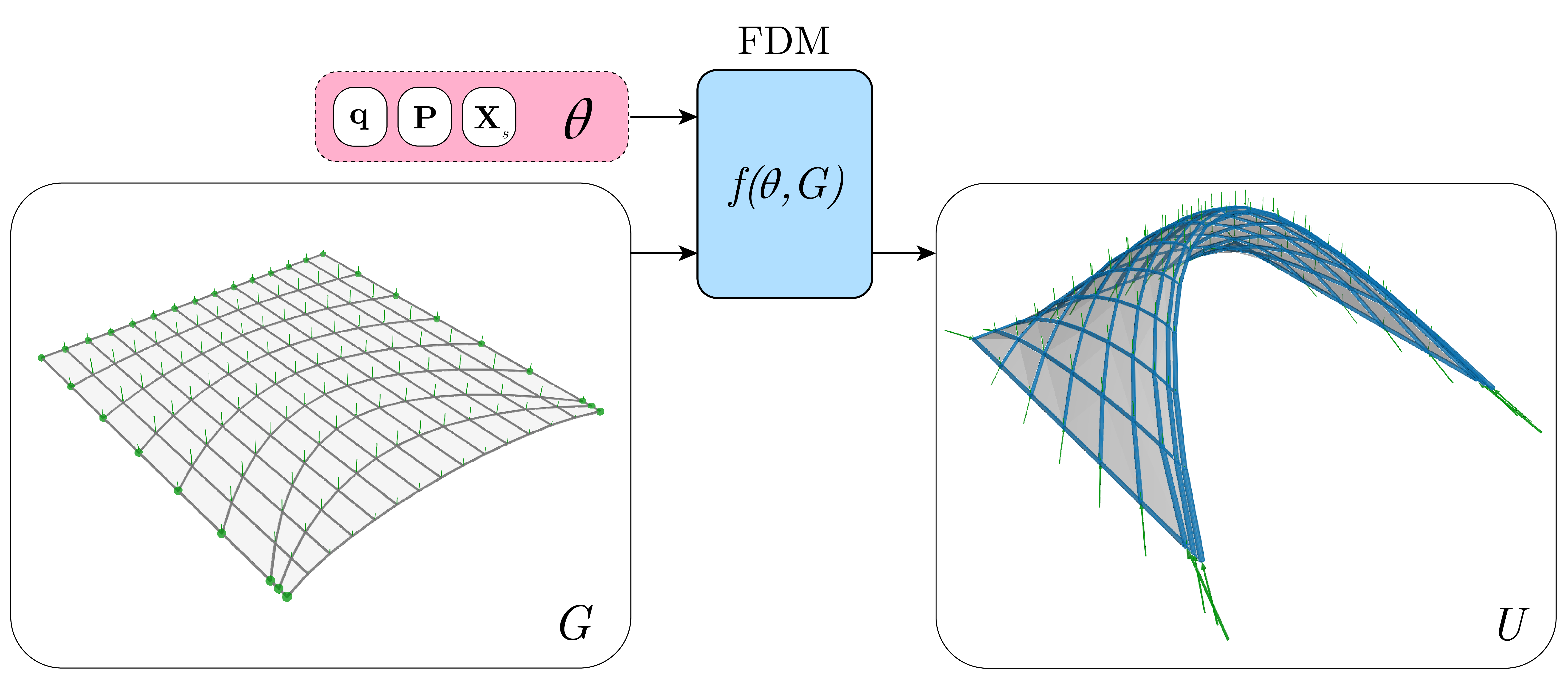
Figure 2: The FDM is a forward form-finding method that computes a state of static equilibrium $U$ on an input graph $G$ given input parameters $\theta=(\mathbf{q},\mathbf{P},\mathbf{X}_{\text{s}})$.

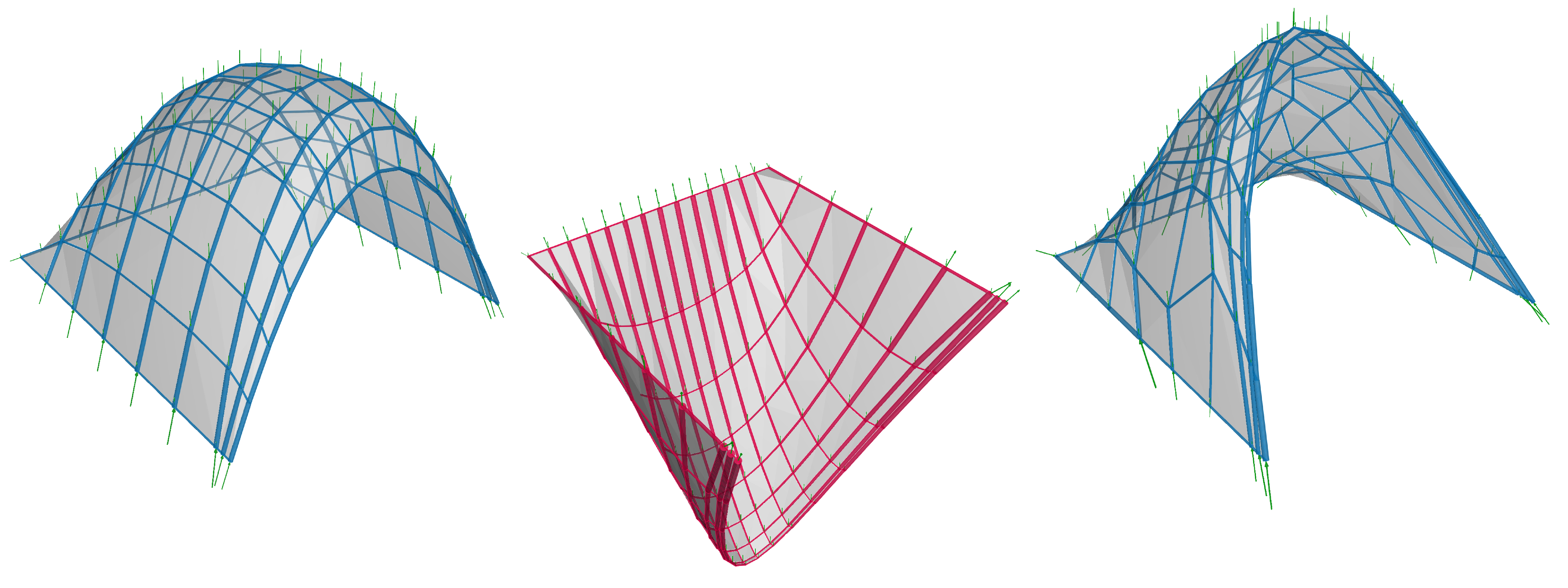
Figure 3: The FDM generates different static equilibrium configurations for variations of $\theta$. From left to right: $\mathbf{q}\in\{-0.1,-1\}$, $\mathbf{q}=\mathbf{1}$, and $\mathbf{q}\sim\mathcal{U}(-0.1,-1)$. Colors indicate the internal axial forces: blue denotes compression and red tension.

2 Auto-differentiable and sparsified FDM

2.1 The force density method (FDM)

The FDM models a structure as a pin-jointed, force network Schek (1974). Let $G=(V,E)$ be a graph with $n$ vertices $V$ connected by $m$ edges $E$ encoding this network. One portion of $V$ of size $n_{s}$ is defined as the supported vertices of the structure $V_{s}$, i.e., the locations in the structure that are fixed and transfer reaction forces to its anchors. The remaining $n_{u}$ unsupported vertices are denoted $V_{u}$.

A connectivity matrix $\mathbf{C}\in\{-1,0,1\}^{m\times n}$ encodes the relationship between the edges and the vertices of $G$. Entry $c_{ij}$ of $\mathbf{C}$ is equal to $1$ if vertex $j$ is the start node of edge $i$ and equal to $-1$ if vertex $j$ is the end node of edge $i$. Otherwise, $c_{ij}=0$. Submatrices $\mathbf{C}_{u}$ and $\mathbf{C}_{s}$ are formed by the columns of $\mathbf{C}$ corresponding to the unsupported and the supported vertices of $G$, respectively.

The FDM is a function $f$ that computes a state of static equilibrium $U$ on a fixed graph $G$ given input parameters $\theta$. The input parameters $\theta=(\mathbf{q},\mathbf{P},\mathbf{X}_{\text{s}})$ are features defined on the elements of $G$:

• A diagonal matrix $\mathbf{Q}\in\mathbb{R}^{m\times m}$ with the force densities of the edges, $\mathbf{q}\in\mathbb{R}^{m\times 1}$. The force density $q_{i}$ of edge $i$ is the ratio between the internal force $t_{i}$ and the length $l_{i}$ of the edge, $q_{i}=t_{i}/l_{i}$. A negative $q_{i}$ indicates compression while a positive one indicates tension.

• A matrix $\mathbf{P}\in\mathbb{R}^{n\times 3}$ with the 3D vectors denoting the external loads applied to all the vertices of $G$. Submatrices $\mathbf{P}_{u}\in\mathbb{R}^{n_{u}\times 3}$ and $\mathbf{P}_{s}\in\mathbb{R}^{n_{s}\times 3}$ correspond to the rows of $\mathbf{P}$ with the loads applied to the vertices $V_{u}$ and $V_{s}$, respectively.

• A matrix $\mathbf{X}_{s}\in\mathbb{R}^{n_{s}\times 3}$ containing the 3D coordinates of the supported vertices, $V_{s}$.

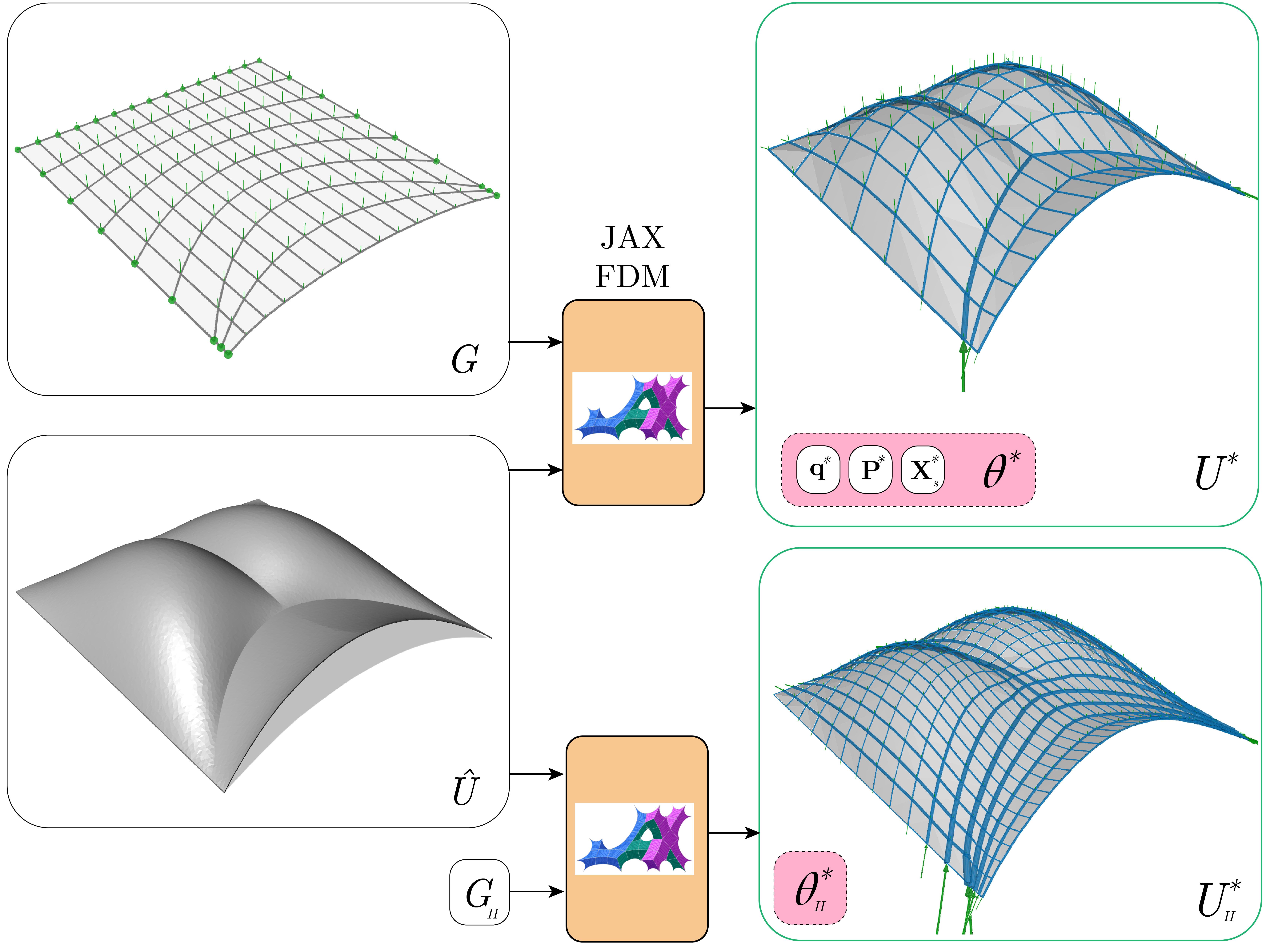
Figure 4: JAX FDM solves inverse form-finding problems estimating parameters $\theta^{\star}$ that fit a prescribed equilibrium state $\hat{U}$ via gradient-based optimization. Here, we calculate the force densities $\mathbf{q}^{\star}$ needed to solve a shape approximation problem on a creased shell modeled as graphs $G$ and $G_{II}$.

The state $U=(\mathbf{X}_{u},\mathbf{R}_{s},\mathbf{t},\mathbf{l})$ characterizes the static equilibrium configuration of $G$:

• A matrix $\mathbf{X}_{u}\in\mathbb{R}^{n_{u}\times 3}$ containing the 3D coordinates in static equilibrium of the unsupported vertices, $V_{u}$.

• A matrix $\mathbf{R}_{s}\in\mathbb{R}^{n_{s}\times 3}$ with the reaction forces incident to the supported vertices, $V_{s}$.

• A vector $\mathbf{t}\in\mathbb{R}^{m\times 1}$ containing the tensile or compressive internal force of the edges.

• A vector $\mathbf{l}\in\mathbb{R}^{m\times 1}$ with the edge lengths.

The key step in the FDM is to find the 3D coordinates in static equilibrium of the free vertices $\mathbf{X}_{u}$ with Eq. 1:

$$\mathbf{X}_{u}=(\mathbf{C}_{u}^{\text{T}}\mathbf{Q}\mathbf{C}_{u})^{-1}(\mathbf{P}_{u}-\mathbf{C}_{u}^{\text{T}}\mathbf{Q}\mathbf{C}_{s}\mathbf{X}_{s})\,$$ (1)

The remaining components of $U$ are computed as:

$$\mathbf{R}_{s} =\mathbf{P}_{s}-\mathbf{C}_{s}^{\text{T}}\mathbf{Q}\mathbf{C}\mathbf{X}$$ (2)

$$\mathbf{t} =\mathbf{q}^{\text{T}}\mathbf{L}$$ (3)

The matrix of 3D coordinates $\mathbf{X}$ results from concatenating $\mathbf{X}_{u}$ and $\mathbf{X}_{s}$. The diagonal matrix of edge lengths $\mathbf{L}$ can be calculated taking the row-wise L2 norm of the inner product of the connectivity matrix $\mathbf{C}$ and $\mathbf{X}$, $\mathbf{L}=\text{diag}(\lVert\mathbf{C}\,\mathbf{X}\rVert_{2})$.

2.2 Solving inverse form-finding problems

The desideratum is to design structures in static equilibrium that attain additional architectural, fabrication, or other target properties.

The FDM parametrizes form-finding in terms of $\theta$, simplifying the computation of a state of static equilibrium $U$ to the solution of a linear system. However, the relationship between $\theta$ and $U$ is non-linear as linear perturbations in $\theta$ do not correspond to linear changes in $U$. Moreover, the force densities $\mathbf{q}$ are not interpretable quantities: they express a ratio between the expected forces and lengths in the edges of a structure, but neither of them concretely. Both issues complicate tackling inverse form-finding problems without an automated approach.

To address these challenges, we solve an unconstrained optimization problem w.r.t. parameters $\theta$. Let $g(f(\theta,G))$ be a non-linear goal function that computes a property of interest. One inverse form-finding problem may contain $K$ different goal functions that are individually scaled by a weight factor $w_{k}$ and aggregated in a loss function $\mathcal{L}(\theta)$:

$$\mathcal{L}(\theta)=\sum_{k=1}^{K}w_{k}\,g_{k}(f(\theta,G)))$$ (4)

We minimize Eq. 4 by estimating optimal parameters $\theta^{\star}$ via gradient descent, iteratively updating $\theta$ in the negative direction of the gradient $\nabla_{\theta}\mathcal{L}$. We conveniently estimate the required value of $\nabla_{\theta}\mathcal{L}$ with reverse-mode automatic differentiation Bradbury et al. (2018).

2.3 Differentiable sparse solver

A bottleneck in our solver is the solution of the linear system in Eq. 1. Although for small problems we can materialize and invert the full dense coefficient matrix $\mathbf{C}_{u}^{T}\mathbf{Q}\mathbf{C}_{u}$, for larger problems we want to take advantage of the inherent sparsity of $\mathbf{C}_{u}$ to get computational speedup, especially as the linear solve is called many times during inverse design.

As sparse solvers have limited support on JAX at the time of writing, we use implicit differentiation to derive a custom differentiable sparse linear solver. Given that the sparsity pattern only depends on $\mathbf{C}$, which is fixed from the beginning for a given graph $G$, we implement a differentiable map from force densities into the entries of the coefficient matrix in compressed sparse-row (CSR) format. We then use the adjoint method to implement a custom gradient for scipy.sparse.linalg.spsolve on CPU, and jax.experimental.sparse.linalg.spsolve on GPU. On CPU, we use a jax.pure_callback to ensure the sparse solve is compatible with JIT compilation.

3 Examples

JAX FDM features a rich bank of goal functions that simplify the modeling of inverse-form-finding problems on various structural systems (Fig. 5). Here, we present two specific use cases with the current version of the library.

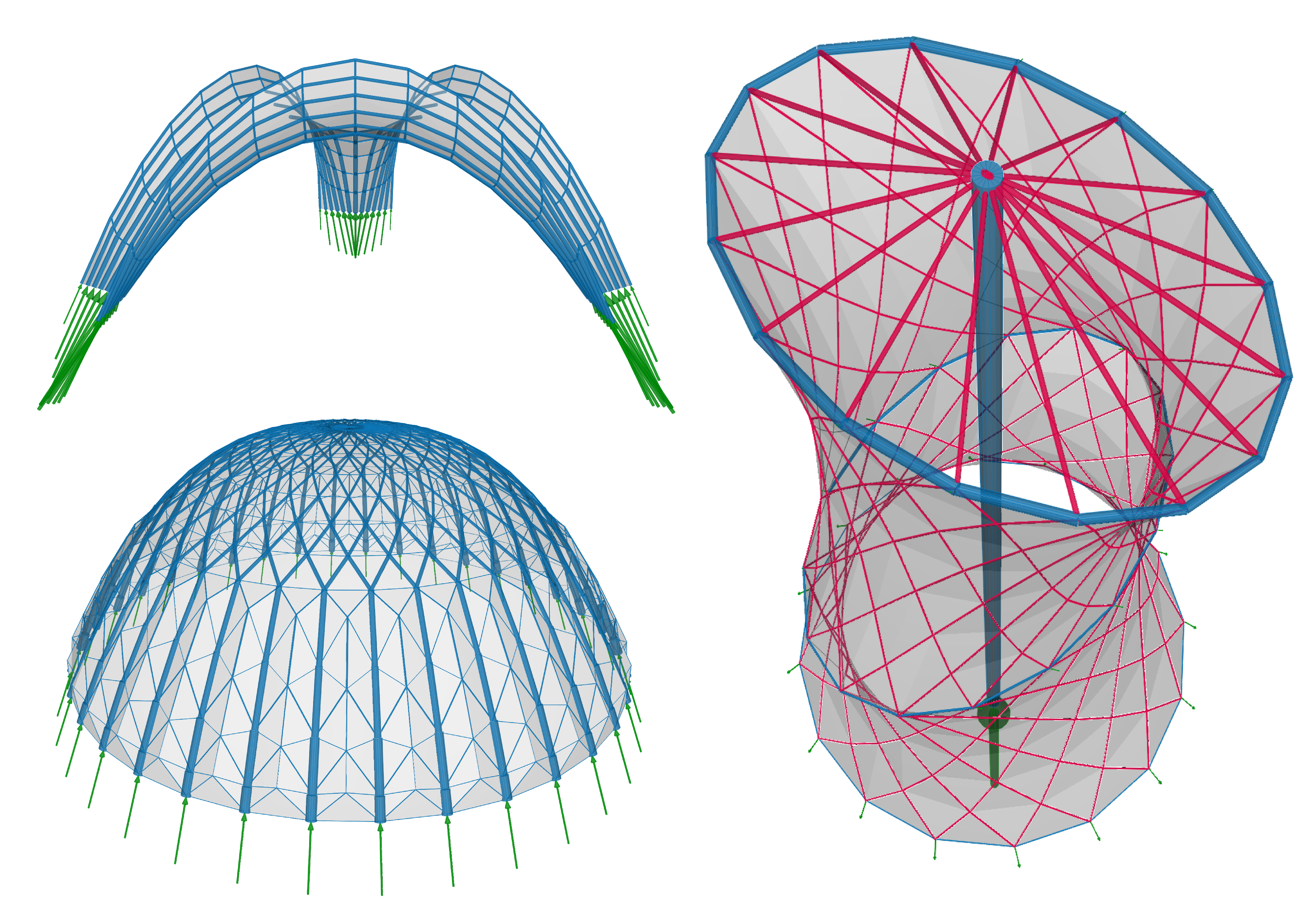
Figure 5: Inverse form-found structures generated with JAX FDM. Left: two compression-only structures, a monkey saddle (top) and a dome (bottom). Right: a tensegrity tower.

3.1 Shape approximation for shell structures

We want to calculate a network in static equilibrium for a shell that approximates the geometry $\hat{U}$ pictured in Fig. 4 Panozzo et al. (2013). This target shape is supplied by the project architect as a COMPAS network Van Mele & many others (2017). JAX FDM offers functions to convert such a network into a JAX-friendly jfe.EquilibriumStructure. This structure encodes the graph representation $G$ of the shell and its connectivity matrix $\mathbf{C}$ (Section 2.1).

⬇

import jax_fdm.equilibrium as jfe

from jax_fdm.datastructures import FDNetwork

# load a structure from a COMPAS network

net = FDNetwork.from_json(”shell.json”)

eqs = jfe.EquilibriumStructure

structure = eqs.from_network(net)

import jax.numpy as jnp

# set the initial force densities

q = jnp.ones(structure.num_edges) * -1.0

# compute an equilibrium state

fdm = jfe.EquilibriumModel()

params = (q, xyz_fixed, loads)

eq_state = fdm(params, structure)

# define loss and target functions

def goal_fn(eq_state):

dist = (eq_state.xyz - xyz_target)**2

return jnp.sum(dist)

def loss_fn(q):

params = (q, xyz_fixed, loads)

eq_state = fdm(params, structure)

return goal_fn(eq_state)

import optax

from jax import jit

from jax import value_and_grad

@jit

def opt_step(q, o_state):

loss, grad = value_and_grad(loss_fn)(q)

upd, o_state = opt.update(grad, o_state)

q = optax.apply_updates(q, upd)

return q, o_state, loss

# optimization loop

opt = optax.adam(learning_rate=0.01)

o_state = opt.init(q)

for i in range(5000):

q, o_state, loss = opt_step(q, o_state)

To compute a state of static equilibrium eq_state with the FDM, we instantiate an jfe.EquilibriumModel and define $\theta$ as a tuple of design parameters, params.

⬇

import jax_fdm.equilibrium as jfe

from jax_fdm.datastructures import FDNetwork

# load a structure from a COMPAS network

net = FDNetwork.from_json(”shell.json”)

eqs = jfe.EquilibriumStructure

structure = eqs.from_network(net)

import jax.numpy as jnp

# set the initial force densities

q = jnp.ones(structure.num_edges) * -1.0

# compute an equilibrium state

fdm = jfe.EquilibriumModel()

params = (q, xyz_fixed, loads)

eq_state = fdm(params, structure)

# define loss and target functions

def goal_fn(eq_state):

dist = (eq_state.xyz - xyz_target)**2

return jnp.sum(dist)

def loss_fn(q):

params = (q, xyz_fixed, loads)

eq_state = fdm(params, structure)

return goal_fn(eq_state)

import optax

from jax import jit

from jax import value_and_grad

@jit

def opt_step(q, o_state):

loss, grad = value_and_grad(loss_fn)(q)

upd, o_state = opt.update(grad, o_state)

q = optax.apply_updates(q, upd)

return q, o_state, loss

# optimization loop

opt = optax.adam(learning_rate=0.01)

o_state = opt.init(q)

for i in range(5000):

q, o_state, loss = opt_step(q, o_state)

The fdm model is a callable object that expresses $f(\theta,G)$ and implements Eqs. 1-3. The initial vector of force densities is set to $\mathbf{q}=-\mathbf{1}$. The negative values denote compressive internal forces in the edges of $G$. The other arrays, xyz_fixed and loads, store the 3D coordinates of the supports $\mathbf{X}_{s}$, and the loads $\mathbf{P}$ applied to the vertices of $G$, respectively. Next, we set up an inverse form-finding problem in terms of $\mathbf{q}$ with two functions:

⬇

import jax_fdm.equilibrium as jfe

from jax_fdm.datastructures import FDNetwork

# load a structure from a COMPAS network

net = FDNetwork.from_json(”shell.json”)

eqs = jfe.EquilibriumStructure

structure = eqs.from_network(net)

import jax.numpy as jnp

# set the initial force densities

q = jnp.ones(structure.num_edges) * -1.0

# compute an equilibrium state

fdm = jfe.EquilibriumModel()

params = (q, xyz_fixed, loads)

eq_state = fdm(params, structure)

# define loss and target functions

def goal_fn(eq_state):

dist = (eq_state.xyz - xyz_target)**2

return jnp.sum(dist)

def loss_fn(q):

params = (q, xyz_fixed, loads)

eq_state = fdm(params, structure)

return goal_fn(eq_state)

import optax

from jax import jit

from jax import value_and_grad

@jit

def opt_step(q, o_state):

loss, grad = value_and_grad(loss_fn)(q)

upd, o_state = opt.update(grad, o_state)

q = optax.apply_updates(q, upd)

return q, o_state, loss

# optimization loop

opt = optax.adam(learning_rate=0.01)

o_state = opt.init(q)

for i in range(5000):

q, o_state, loss = opt_step(q, o_state)

The first one is a goal function $g(f(\theta,G))$, which quantifies the fitness of the shape approximation by measuring the cumulative distance between the xyz coordinates in static equilibrium of the vertices $V$ produced by fdm, and the xyz_target coordinates on the objective surface. The second function represents Eq. 4, which we minimize with an optax optimizer Babuschkin et al. (2020):

⬇

import jax_fdm.equilibrium as jfe

from jax_fdm.datastructures import FDNetwork

# load a structure from a COMPAS network

net = FDNetwork.from_json(”shell.json”)

eqs = jfe.EquilibriumStructure

structure = eqs.from_network(net)

import jax.numpy as jnp

# set the initial force densities

q = jnp.ones(structure.num_edges) * -1.0

# compute an equilibrium state

fdm = jfe.EquilibriumModel()

params = (q, xyz_fixed, loads)

eq_state = fdm(params, structure)

# define loss and target functions

def goal_fn(eq_state):

dist = (eq_state.xyz - xyz_target)**2

return jnp.sum(dist)

def loss_fn(q):

params = (q, xyz_fixed, loads)

eq_state = fdm(params, structure)

return goal_fn(eq_state)

import optax

from jax import jit

from jax import value_and_grad

@jit

def opt_step(q, o_state):

loss, grad = value_and_grad(loss_fn)(q)

upd, o_state = opt.update(grad, o_state)

q = optax.apply_updates(q, upd)

return q, o_state, loss

# optimization loop

opt = optax.adam(learning_rate=0.01)

o_state = opt.init(q)

for i in range(5000):

q, o_state, loss = opt_step(q, o_state)

The object abstractions and equilibrium calculations in JAX FDM are compatible with JAX transformations, such as jit and value_and_grad. This compatibility allows us to write the optimization step for $\mathbf{q}$ with the same code blocks conventionally used to train neural networks.

Post-optimization, the distance between the solution provided by $\mathbf{q}^{\star}$ and the target shape decreases by four orders of magnitude. The fit is comparable with an input graph $G_{II}$ that has three times more edges and design parameters (Fig. 4). This example is available in a Colab notebook at https://tinyurl.com/25czahvh.

3.2 Equalizing edge lengths in a cable net

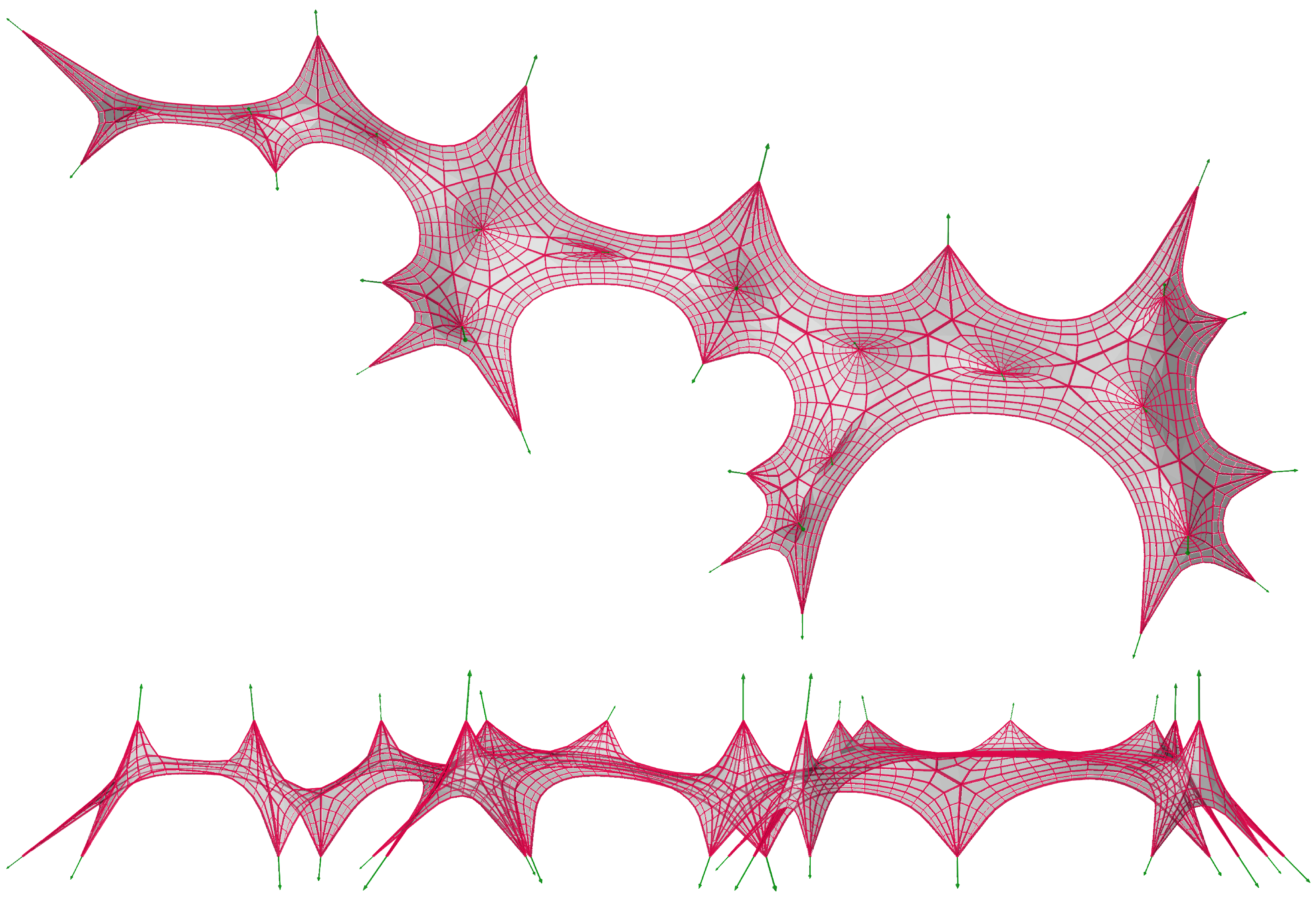
Figure 6: A cable net roof. The cables of this inverse form-found, tension-only structure have a target length of $0.15$ m.

We design a self-stressed cable net inspired by the roof of the Rhön Klinikum Oval (2019). Building cable nets from standardized components is important for fabrication efficiency. Therefore, we calculate a tension-only shape for the net that has a target edge length of $0.15$ m. Fig. 6 displays the solution to the inverse form-finding problem. The goal function $g(f(\theta,G))$ in this problem is:

⬇

# define target functions

def goal_fn(eq_state):

diff = (eq_state.lengths - 0.15)**2

std = jnp.std(eq_state.lengths)

return jnp.sum(diff) + 0.01 * std

After modeling the connectivity of the cable net as a structure, we can reuse the code blocks presented in Section 3.1 to obtain $\mathbf{q}^{\star}$. The only requirement is to swap goal_fn in the body of the loss function loss_fn. The composition and interchangeability of such atomic goal functions simplify the formulation of custom inverse form-finding problems with JAX FDM. We applied a similar approach to generate the planar cable net shown in Fig. 1.

4 Conclusion

We presented JAX FDM, an open-source solver that streamlines the design of 3D structures in static equilibrium conditioned on target properties. Future work will include our solver as a differentiable layer in neural networks to build accurate surrogate models that further accelerate inverse form-finding.

References

- Adriaenssens et al. (2014) Adriaenssens, S., Block, P., Veenendaal, D., and Williams, C. (eds.). Shell structures for architecture: form finding and optimization. Routledge/ Taylor & Francis Group, London ; New York, 2014. ISBN 978-0-415-84059-0 978-0-415-84060-6. URL https://doi.org/10.4324/9781315849270.
- Babuschkin et al. (2020) Babuschkin, I., Baumli, K., Bell, A., Bhupatiraju, S., Bruce, J., Buchlovsky, P., Budden, D., Cai, T., Clark, A., Danihelka, I., Dedieu, A., Fantacci, C., Godwin, J., Jones, C., Hemsley, R., Hennigan, T., Hessel, M., Hou, S., Kapturowski, S., Keck, T., Kemaev, I., King, M., Kunesch, M., Martens, L., Merzic, H., Mikulik, V., Norman, T., Papamakarios, G., Quan, J., Ring, R., Ruiz, F., Sanchez, A., Schneider, R., Sezener, E., Spencer, S., Srinivasan, S., Stokowiec, W., Wang, L., Zhou, G., and Viola, F. The DeepMind JAX Ecosystem, 2020. URL http://github.com/deepmind.
- Bradbury et al. (2018) Bradbury, J., Frostig, R., Hawkins, P., Johnson, M. J., Leary, C., Maclaurin, D., and Wanderman-Milne, S. JAX: composable transformations of Python+NumPy programs, 2018. URL http://github.com/google/jax.
- Chang & Cheng (2020) Chang, K.-H. and Cheng, C.-Y. Learning to simulate and design for structural engineering. In III, H. D. and Singh, A. (eds.), Proceedings of the 37th international conference on machine learning, volume 119 of Proceedings of machine learning research, pp. 1426–1436. PMLR, July 2020. URL http://proceedings.mlr.press/v119/chang20a.html.
- Cuvilliers (2020) Cuvilliers, P. The constrained geometry of structures: Optimization methods for inverse form-finding design. PhD Thesis, Massachusetts Institute of Technology., 2020. URL http://dspace.mit.edu/handle/1721.1/7582.
- Koohestani (2012) Koohestani, K. Form-finding of tensegrity structures via genetic algorithm. International Journal of Solids and Structures, 49(5):739–747, March 2012. ISSN 0020-7683. URL http://doi.org/10.1016/j.ijsolstr.2011.11.015.
- Lee et al. (2016) Lee, J., Mueller, C., and Fivet, C. Automatic generation of diverse equilibrium structures through shape grammars and graphic statics. International Journal of Space Structures, 31(2-4):147–164, June 2016. ISSN 0266-3511. URL http://doi.org/10.1177/0266351116660798.
- Marmo et al. (2019) Marmo, F., Masi, D., Mase, D., and Rosati, L. Thrust network analysis of masonry vaults. International Journal of Masonry Research and Innovation, 4(1/2):64, 2019. ISSN 2056-9459, 2056-9467. URL http://www.doi.org/10.1504/IJMRI.2019.096828.
- Oval (2019) Oval, R. Topology Finding of Patterns for Structural Design. PhD Thesis, École des Ponts ParisTech, Paris, France, 2019. URL https://theses.hal.science/tel-02917467.
- Panozzo et al. (2013) Panozzo, D., Block, P., and Sorkine-Hornung, O. Designing Unreinforced Masonry Models. ACM Transactions on Graphics - SIGGRAPH 2013, 32(4):91:1–91:12, 2013. URL http://doi.org/10.1145/2461912.2461958.
- Pastrana et al. (2023) Pastrana, R., Ohlbrock, P. O., Oberbichler, T., D’Acunto, P., and Parascho, S. Constrained Form-Finding of Tension–Compression Structures using Automatic Differentiation. Computer-Aided Design, 155:103435, 2023. ISSN 0010-4485. URL http://doi.org/10.1016/j.cad.2022.103435.
- Rippmann et al. (2016) Rippmann, M., Popescu, M., Augustynowicz, E., Méndez Echenagucia, T., Calvo Barentin, C., Frick, U., Van Mele, T., and Block, P. The Armadillo Vault: Computational Design and Digital Fabrication of a Freeform Stone Shell. In Advances in Architectural Geometry 2016, pp. 344–363, Zurich, Switzerland, 2016. vdf Hochschulverlag AG an der ETH Zürich. URL http://doi.org/10.3218/3778-4_23.
- Schek (1974) Schek, H.-J. The force density method for form finding and computation of general networks. Computer Methods in Applied Mechanics and Engineering, 3(1):115–134, January 1974. ISSN 0045-7825. URL http://doi.org/10.1016/0045-7825(74)90045-0.
- Schlaich (2018) Schlaich, M. Shell Bridges - and a New Specimen Made of Stainless Steel. Journal of the International Association for Shell and Spatial Structures, 59(3):215–224, September 2018. ISSN 1028-365X. URL http://doi.org/10.20898/j.iass.2018.197.027.
- Van Mele & many others (2017) Van Mele, T. and many others. COMPAS: A framework for computational research in architecture and structures., 2017. URL https://doi.org/10.5281/zenodo.2594510.
- Veenendaal et al. (2017) Veenendaal, D., Bakker, J., and Block, P. Structural Design of the Flexibly Formed, Mesh-Reinforced Concrete Sandwich Shell Roof of NEST HiLo. Journal of the International Association for Shell and Spatial Structures, 58(1):23–38, March 2017. ISSN 1028365X, 19969015. URL http://doi.org/10.20898/j.iass.2017.191.847.
- Wu (2023) Wu, G. A framework for structural shape optimization based on automatic differentiation, the adjoint method and accelerated linear algebra. Structural and Multidisciplinary Optimization, 66(7):151, June 2023. ISSN 1615-1488. URL https://doi.org/10.1007/s00158-023-03601-0.
- Xue et al. (2023) Xue, T., Liao, S., Gan, Z., Park, C., Xie, X., Liu, W. K., and Cao, J. JAX-FEM: A differentiable GPU-accelerated 3D finite element solver for automatic inverse design and mechanistic data science. Computer Physics Communications, 291:108802, October 2023. ISSN 0010-4655. URL http://doi.org/10.1016/j.cpc.2023.108802.
- Zhang & Ohsaki (2006) Zhang, J. Y. and Ohsaki, M. Adaptive force density method for form-finding problem of tensegrity structures. International Journal of Solids and Structures, 43(18):5658–5673, September 2006. ISSN 0020-7683. URL http://doi.org/10.1016/j.ijsolstr.2005.10.011.