Optimal Control of Multiclass Fluid Queueing Networks: A Machine Learning Approach

Abstract

We propose a machine learning approach to the optimal control of multiclass fluid queueing networks (MFQNETs) that provides explicit and insightful control policies. We prove that a threshold type optimal policy exists for MFQNET control problems, where the threshold curves are hyperplanes passing through the origin. We use Optimal Classification Trees with hyperplane splits (OCT-H) to learn an optimal control policy for MFQNETs. We use numerical solutions of MFQNET control problems as a training set and apply OCT-H to learn explicit control policies. We report experimental results with up to 33 servers and 99 classes that demonstrate that the learned policies achieve 100% accuracy on the test set. While the offline training of OCT-H can take days in large networks, the online application takes milliseconds.

1 Introduction

Multiclass queueing networks (MQNETs) are complex systems that model the behavior of multiple classes of jobs, each with their own arrival and service rates, routing paths and holding costs. These networks find numerous applications in diverse fields, including manufacturing (Kumar, 1993), healthcare (Cochran & Roche, 2009) and communication networks (Srikant & Ying, 2014) among many. The control of MQNETs is of great importance in improving system efficiency, optimizing resource allocation, and reducing operational costs. However, the inherent complexity of these systems makes their analysis and control a challenging task.

Multiclass fluid queueing networks (MFQNETs) have been developed as a deterministic, continuous approximation of MQNETs, primarily to provide a tractable method for analyzing the stability of the underlying MQNETs. (Dai, 1995; Stolyar, 1995) demonstrate that the stability of MFQNETs implies the stability of underlying MQNETs. Several related studies including (Meyn, 1995; Dumas, 1999; Gamarnik & Hasenbein, 2005) have also explored the topic. See (Bertsimas & Gamarnik, 2022) for a comprehensive review.

MFQNETs also provide a useful way to construct control policies for MQNETs as the optimal control of MFQNETs is often much more tractable than the optimal control of underlying MQNETs. To this end, several approaches have been proposed in the literature. (Maglaras, 1999, 2000) propose discrete review policies and show that they achieve asymptotic optimality and stability under fluid scailing. (Bertsimas et al., 2015) provide a robust formulation of MFQNET control problem and translate the resulting policy to the underlying MQNET. (Bertsimas & Sethuraman, 2002; Dai & Weiss, 2002) propose methods to approximately minimize make-span based on the associated fluid models. For a comprehensive review of the topic, see (Meyn, 2007) and (Bertsimas & Gamarnik, 2022).

Mathematically, optimal control of MFQNETs falls into a subclass of infinite dimensional linear optimization models known as separated continuous linear programs (SCLPs). Several researchers have investigated the theoretical properties of SCLPs, such as (Anderson et al., 1983; Pullan, 1995, 1996, 1997). (Avram et al., 1995) find closed-form optimal policies for specific MFQNETs using optimality conditions from optimal control theory. Other works have proposed numerical algorithms for solving SCLPs. (Pullan, 1993, 2002; Luo & Bertsimas, 1998) develop algorithms based on discretization, while (Weiss, 2008; Shindin et al., 2021) propose simplex-like methods. (Fleischer & Sethuraman, 2005; Bampou & Kuhn, 2012) propose polynomial-time approximation algorithms.

Despite significant efforts in the field and its practical applications, optimal control of MFQNETs remains a challenging computational task. Moreover, current algorithms typically provide only numerical solutions, making it difficult to gain insight into the underlying structure of the optimal policy.

Recently, there has been growing interest in applying machine learning techniques to solve challenging optimization and control problems. For instance, (Khalil et al., 2016; Alvarez et al., 2017; Bertsimas & Kim, 2023b; Bertsimas & Stellato, 2021, 2022; Cauligi et al., 2022) propose machine learning-based approaches to mixed-integer optimization. Bertsimas & Kim (2023a) develop a method to solve two-stage adaptive robust optimization problems using machine learning. Machine learning has been used for hyperparameter tuning in optimization algorithms as well (Hutter et al., 2011; Balcan et al., 2020). For queueing network control, reinforcement learning methods are proposed in (Raeis et al., 2021; Liu et al., 2019; Dai & Gluzman, 2022). Although these approaches have shown to be effective in addressing computational challenges, it can be difficult to provide theoretical guarantees that the machine learning methods lead to optimal solutions.

In this paper, we present a novel approach that leverages machine learning to solve MFQNET control problems. The MFQNET control problem we consider is the fluid analog of the sequencing problem in MQNETs. The sequencing problem in MQNETs is a stochastic and discrete control problem that involves deciding which class of jobs to process at each server at any given time, with the aim of minimizing the expected total cost. We formulate the fluid analog of this problem as a SCLP problem and propose a machine learning-based algorithm to address it.

We solve multiple MFQNET control problems and use the resulting numerical solutions to learn an optimal policy. The machine learning algorithm we use is Optimal Classification Trees with hyperplane splits (OCT-H) proposed by (Bertsimas & Dunn, 2017, 2019). OCT-H is a classification algorithm that partitions the feature space using hyperplanes and assigns a prediction to each region. We prove that OCT-H can learn exact optimal policies for the MFQNET control problems.

The contributions of the paper are as follows.

1. We prove the existence of a threshold-type optimal policy for MFQNET control problems, where the threshold curves are hyperplanes passing through the origin. This result was previously proven only for special cases.

2. Based on the theoretical findings, we propose an efficient algorithm that can learn an exact optimal control policy for MFQNETs using OCT-H. We report experimental results with up to 33 servers and 99 classes that demonstrate that the learned policies achieve 100% accuracy on the test set.

3. Once a policy is learned offline, it can be directly applied online to unseen states in milliseconds, leading to a significant speed-up compared to solving the problem numerically.

4. The high interpretability of decision trees allows us to gain insights into the structure of the optimal policy, which is a significant advantage that numerical optimization algorithms often lack. By providing the actual decision trees learned by OCT-H, we develop a deeper understanding of MFQNETs and their optimal policy.

The structure of this paper is as follows. Section 2 provides the definition of MFQNET control, along with the associated optimality conditions. We also provide a brief review of OCT-H. Section 3 provides our theoretical results on the structure of optimal policy for MFQNET control. We then develop a learning algorithm based on OCT-H and provide a small example to illustrate the method. Section 4 reports the results of computational experiments, where we analyze the accuracy, speed, and interpretability of our approach.

Notational conventions

Throughout this paper, we use lower case boldface letters to denote vectors and upper case boldface letters to denote matrices. The $i_{th}$ entry of a vector $\bm{x}$ is denoted $x_{i}$, and the entry in the $i_{th}$ row and $j_{th}$ column of a matrix $\bm{A}$ is denoted $a_{ij}$. Division between two vectors is always assumed to be entry-wise. We use $\bm{e}$ to denote the vector of all ones and $\bm{0}$ to denote the vector of zeros. We use $x(\cdot)$ to denote a real-valued function, and $\bm{x}(\cdot)$ to denote a vector whose entries are real-valued functions. We use $\bm{x}$ instead of $\bm{x}(\cdot)$ when it is clear from the context that $\bm{x}$ is referring to a vector of functions.

2 Background

In this section, we first define the optimal control problem for MFQNETs. Then, we review necessary optimality conditions in optimal control theory and provide a brief overview of OCT-H.

2.1 Optimal Control of MFQNETs

Consider a queueing network with $m$ servers and $n$ job classes. Each job class $i\in[n]$ is processed by a single server $s(i)\in[m]$ with service rate $\mu_{i}$. After jobs of class $i$ are processed, they either leave the system or change to a different class in a deterministic manner. Jobs may arrive from either another server or from outside the system with external arrival rate $\lambda_{i}$. If there is no external arrival for class $i$, then $\lambda_{i}=0$. The cost per unit time for holding a job of class $i$ is denoted $c_{i}$.

For each class $i\in[n]$, the control variable $u_{i}(t)$ denotes the fraction of effort the server $s(i)$ spends processing class $i$ jobs at time $t$. The state variable $x_{i}(t)$ is the number of jobs of class $i$ at time $t$. The dynamics of the system can be expressed using a matrix $\bm{A}\in\mathbb{R}^{n\times n}$, where $a_{ii}=-\mu_{i}$ and ${a}_{ij}=\mu_{j}$ if class $i$ receives arrivals from class $j,\;j\neq i$. The rest of the entries of $\bm{A}$ are zero. Then, the dynamics of the system is

$$\dot{\bm{x}}(t)=\bm{A}\bm{u}(t)+\bm{\lambda}.$$

In addition, the sum of the control variables for all classes that are processed at the same server should be less than or equal to one. This constraint can be expressed as

$$\bm{D}\bm{u}(t)\leq\bm{e},$$

where $\bm{D}\in\{0,1\}^{m\times n}$ is a binary matrix with $d_{ij}=1$ if $s(j)=i$ and $d_{ij}=0$, otherwise.

The MFQNET control problem aims to find a control $\bm{u}$ that minimizes the total holding cost of the jobs in the system over the time interval $[0,T]$. We define the MFQNET control problem with an initial state $\bm{x}_{0}$ as the following:

$$\underset{\bm{u}(\cdot),\bm{x}(\cdot)}{\min}\quad \int_{0}^{T}\bm{c}^{\top}\bm{x}(t)\,dt$$ (1)

$$s.t. \dot{\bm{x}}(t)=\bm{A}\bm{u}(t)+\bm{\lambda},\quad\forall t\in[0,T],$$

$$\bm{D}\bm{u}(t)\leq\bm{e},\quad\forall t\in[0,T],$$

$$\bm{u}(t),\bm{x}(t)\geq\bm{0},\quad\forall t\in[0,T],$$

$$\bm{x}(0)=\bm{x}_{0}.$$

We use $\bm{u}^{*}_{\bm{x}_{0}}$ and $\bm{x}^{*}_{\bm{x}_{0}}$ to denote the optimal control and the associated state trajectory of problem (1) with the initial state $\bm{x}_{0}$. We use $\bm{u}^{*}$ and $\bm{x}^{*}$ to denote the optimal control and the associated state trajectory of general MFQNET control problems when the initial state is not specified.

We define the workload vector $-\bm{D}\bm{A}^{-1}\bm{\lambda}\in\mathbb{R}^{m}$, and assume that all the entries of the workload vector are strictly smaller than 1 for stability. We further assume $T$ is large enough, so that the system can be emptied by time $T$ (Meyn, 2007). Under this setting, identifying the optimal initial control $\bm{u}^{*}_{\bm{x}_{0}}(0)$ for any initial state $\bm{x}_{0}$ is equivalent to identifying the optimal policy $\bm{u}^{*}(t)$ for any state $\bm{x}(t)$.

2.2 Optimality Conditions of MFQNET Control

The Pontryagin Maximum Principle (Pontryagin et al., 1963; Sethi, 2019) provides necessary optimality conditions for general optimal control problems. Due to the non-negativity constraints on the state variable in Problem (1), the conditions that we provide are tailored for the optimal control problems with pure state constraints.

We define the Hamiltonian of Problem (1) as

$$H(\bm{x},\bm{u},\bm{y},t)=\bm{c}^{\top}\bm{x}(t)+\bm{y}(t)^{\top}[\bm{A}\bm{u}(t)+\bm{\lambda}],$$

where $\bm{y}(t)$ is known as the costate variable.

Lemma 1 (Pontryagin Maximum Principle (Pontryagin et al., 1963; Sethi, 2019))

If the feasible control ${\bm{u}^{*}}$ and the state trajectory ${\bm{x}^{*}}$ is optimal for Problem (1), there exists ${\bm{y}}(t)$ for any $t\in[0,T]$ that satisfies the following conditions.

1. $H(\bm{x}^{*},\bm{u}^{*},\bm{y},t)\leq H(\bm{x}^{*},\bm{u},\bm{y},t)$ for all $\bm{u}(t)$ satisfying $\bm{u}(t)\geq\bm{0}$, $\bm{D}\bm{u}(t)\leq\bm{e}$.

2. Whenever ${\bm{u}}^{*}(t)$ is continuous, $\dot{\bm{y}}(t)=-\bm{c}+\bm{\pi}(t),$ where $\bm{\pi}(t)\geq\bm{0},\bm{\pi}(t)^{\top}{\bm{x}^{*}}(t)=0$.

3. $\bm{y}(T)=\bm{0}$.

Proof 1

See (Sethi, 2019).

2.3 Optimal Classification Trees with Hyperplane Splits

Optimal Classification Trees (OCT) is an algorithm to learn near-optimal decision trees for classification tasks. Classification and Regression Trees (CART) (Brieman et al., 1984), an earlier algorithm to learn decision trees for prediction tasks, learns a decision tree in a greedy manner using recursive partitioning of the feature space at each child node. However, OCT aims to learn a globally optimal decision tree using mixed-integer optimization and local heuristics.

Similar to CART and other classification algorithms, OCT takes $N$ data inputs $\{(\bm{\theta}_{i},z_{i})\}_{i=1}^{N}$, where $\bm{\theta}_{i}$ is the feature vector and $z_{i}$ is the label for the $i_{th}$ data point. Given this data set, OCT learns a decision tree that uses a single feature for the split at each node and assigns a label to each node of the tree. Given a new data point $\bm{\theta}_{0}$, it traverses the decision tree until it reaches a leaf node. The prediction of the tree for $\bm{\theta}_{0}$ is the label assigned to the leaf node.

OCT-H, a generalization of OCT, can use an arbitrary linear combination of the features for splits at the nodes. This means that OCT-H can use general hyperplanes for splits, whereas OCT is confined to use hyperplanes that are perpendicular to the axes in the feature space. Essentially, OCT-H partitions the feature space with hyperplanes, and assigns a prediction to each region. This observation is the key to our work to solve Problem (1) using OCT-H. Compared to OCT, OCT-H generally shows higher prediction accuracy and learns shallower trees.

In OCT-H, it is possible to limit the number of features that can be used for splits, which can result in a more interpretable tree. This version of OCT-H is denoted as OCT-H with sparsity throughout the remainder of the paper. We simply use OCT-H to denote regular OCT-H, where the entire features can be used. For a more detailed explanation on OCT and OCT-H, we refer readers to Bertsimas & Dunn (2017, 2019).

3 OCT-H for the Optimal Control of MFQNETs

In this section, we first prove that OCT-H can learn an optimal policy of Problem (1). Based on this result, we then proceed to develop an efficient algorithm to learn an optimal policy of Problem (1) using OCT-H.

3.1 Theoretical Results

For each job class $i\in[n]$, we define the depletion time $T_{i}=\inf\{t\in(0,T]:x^{*}_{i}(t)=0\}$ under an optimal state trajectory $\bm{x}^{*}$, assuming that $x_{i}^{*}(0)>0$. The following Lemma will be used to prove our main theorem.

Lemma 2

The costate variable $\bm{y}(t)$ in Lemma 1 satisfies the following statements.

1. If $x_{i}^{*}(t)=0$ for some interval $t\in(\tau_{1},\tau_{2})$, then $y_{i}(t)=0$ for $t\in(\tau_{1},\tau_{2})$.

2. $\bm{y}(t)$ is continuous, piecewise linear function of $t$.

3. At any time $t\in[0,T]$, the value of $\bm{y}(t)$ can be expressed as a linear function of $(T_{1},\dots,T_{n})$.

Proof 2

(a) We consider the relation between the costate variable for the indirect method and the costate variable for the direct method (Sethi, 2019). For optimal control problems with pure state constraints, there are different ways to associate multipliers to the constraints. The method we presented in Section 2.2 is known as the direct method. For the indirect method, the Lagrangian is defined as

$$L(\bm{x},\bm{u},\bm{y},t)=\bm{c}^{\top}\bm{x}(t)+\tilde{\bm{y}}(t)^{\top}[\bm{A}\bm{u}(t)+\bm{\lambda}]+\bm{\eta}(t)^{\top}[\bm{A}\bm{u}(t)+\bm{\lambda}].$$

It is known that $\frac{\partial L}{\partial\bm{u}}\Bigr{|}_{\begin{subarray}{c}\bm{u}=\bm{u}^{*}(t)\end{subarray}}=0$, leading to the equality $(\tilde{\bm{y}}(t)+\bm{\eta}(t))^{\top}\bm{A}=\bm{0}$. As $\bm{A}$ is invertible in our setting, we get $\tilde{\bm{y}}(t)+\bm{\eta}(t)=\bm{0}$. Finally, using the relation between the costate variables for the direct and the indirect method in a boundary interval, we get ${y}_{i}(t)=\tilde{{y}_{i}}(t)+{\eta_{i}}(t)=0,\forall t\in(\tau_{1},\tau_{2})$ (Hartl et al., 1995). For more details on the direct and the indirect method and the associated optimality conditions, we refer readers to (Sethi, 2019).

(b) We define the value function $V(\bm{x})$ as the optimal objective value of Problem (1) associated with the initial state $\bm{x}$. We use the fact that $V(\bm{x})$ is continuously differentiable (Bäuerle, 2001), and the interpretation of the costate variable that $\bm{y}(t)=\frac{\partial V(\bm{x})}{\partial\bm{x}}\Bigr{|}_{\begin{subarray}{c}\bm{x}=\bm{x}^{*}(t)\end{subarray}}$ (Sethi, 2019). Since $\bm{x}^{*}(t)$ is continuous in $t$, the continuity of $\bm{y}(t)$ follows from the continuity of the composition of continuous functions. Piecewise linearity is then straightforward from condition (b) in Lemma 1 and statement (a) in Lemma 2.

(c) This part is implied by the structure of $\bm{y}(t)$ given in the statements (a) and (b) of Lemma 2. Assuming that $x_{i}(0)>0$, $y_{i}(t)$ initially decreases with the slope $-c_{i}$ until the depletion time $T_{i}$, at which $y(T_{i})=0$. For all $t\in[T_{i},T]$, $y_{i}(t)=0$. This fact is implied by condition (c) in Lemma 1 that $\bm{y}(T)=0$. If $x_{i}$ becomes positive again after $T_{i}$, the slope will become $-c_{i}$ as well, making $y_{i}(t)$ negative. Then, it becomes impossible to satisfy ${y}_{i}(T)=0$. Hence, once $x_{i}$ becomes zero, it is kept to zero. A direct consequence is that for all $t\in[T_{i},T]$, $y_{i}(t)=0$ by (a) in Lemma 2. Hence, $y_{i}(t)$ is a linear function of $T_{i}$ for any $t\in[0,T]$.

The following theorem is our main theoretical result that generalizes the results by Avram et al. (1995) to general MFQNETs.

Theorem 3

For Problem (1), there exists a threshold type optimal policy where the threshold curves are hyperplanes passing through the origin.

Proof 3

Our proof is based upon the algorithm by Avram (1997) to solve Problem (1) with any given initial state. We prove that the solution this algorithm finds is a threshold type policy and the threshold curves are hyperplanes passing through the origin.

By condition (a) of Lemma 1, the optimal control at each time $t$ is decided by the priority index $r_{i}(t)$ defined for each job class $i\in[n]$, where $r_{i}(t)=[\bm{y}(t)^{\top}\bm{A}]_{i}$. Lemma 2 indicates that $r_{i}(t)$ is a continuous, piecewise linear function and its slope can only change at $\{T_{1},\dots,T_{n}\}$. At each server, the optimal policy is to put maximum effort to the job class with the smallest priority index, and put zero effort to the rest, without violating the non-negativity constraint on the state variables. When all the job classes at the server have positive priority indices, the optimal policy is to idle. This case can be captured by considering idling as a job class with the constant priority index 0. Hence, Lemma 1 implies that as long as the rank of the priority indices does not change, the optimal control is a constant vector.

The condition under which a server transfers effort from one class to another is defined by the equalities of the form $r_{j}(t)=r_{k}(t)$, given that class $j$ jobs and class $k$ jobs are processed by the same server. If this equality holds, then it is indifferent whether the server prioritizes class $j$ or $k$. If this equality becomes inequality, then it would be beneficial to prioritize one class over the other. This description indicates that the optimal policy is a threshold type policy, and the threshold curves are defined by the equalities between the priority indices.

We derive the condition that the priority is switched from class $j$ jobs to class $k$ jobs, starting from an initial state $\bm{x}_{0}$. Depending on the parameters $\bm{c}$ and $\bm{A}$, certain switches might not be always possible. Furthermore, the order of the depletion times $\{T_{1},\dots,T_{n}\}$ and the future switches associated with the trajectory should be adequately decided as well (Specific examples of how $\bm{A}$, $\bm{c}$ and the order of $\{T_{1},\dots,T_{n}\}$ can make a switch possible or not are given in (Avram et al., 1995; Avram, 1997)). We assume that $\bm{A}$, $\bm{c}$, the order of $\{T_{1},\dots,T_{n}\}$ and the switches associated with the trajectory are appropriately fixed. The specific order of $\{T_{1},\dots,T_{n}\}$ leads to a collection of equalities between the indices $r_{i}(t)$ during the entire trajectory, and completely determines the optimal solution of the problem (Avram et al., 1995; Avram, 1997).

Without loss of generality, we assume that the switch from class $j$ to $k$ happens at $t=0$. The switching curve that we would like to derive is then $r_{j}(0)=r_{k}(0)$, where $r_{j}(0)$ and $r_{k}(0)$ are both linear functions of $(T_{1},\dots,T_{n})$ due to Lemma 2. We now prove that $(T_{1},\dots,T_{n})$ is a linear function of $\bm{x}_{0}$, which verifies that $r_{j}(0)=r_{k}(0)$ represents a hyperplane passing through the origin in the state space.

By definition, $T_{i}$ can be computed from the equation of the form $\int_{0}^{b_{1}}[\bm{A}\bm{u}(t)+\bm{\lambda}]_{i}\,dt+\dots+\int_{b_{q}}^{T_{i}}[\bm{A}\bm{u}(t)+\bm{\lambda}]_{i}\,dt=-x_{i}$, where $b_{l},l\in[q]$, represents a breakpoint in $[\bm{A}\bm{u}(t)+\bm{\lambda}]_{i}$ . The control $[\bm{A}\bm{u}(t)+\bm{\lambda}]_{i}$ is constant between the breakpoints, and the breakpoints $b_{i}$ are always the intersections between two indices. Any time of intersection between two indices can be expressed as a linear function of the vector $(T_{1},\dots,T_{n})$ due to Lemma 2. Hence, the above equation leads to an equality between $x_{i}$ and a linear function of $(T_{1},\dots,T_{n})$. Likewise, the collection of equalities that we have all lead to equalities between $\bm{x}_{0}$ and linear functions of $(T_{1},\dots,T_{n})$. Rearranging these equalities leads to the expression of $(T_{1},\dots,T_{n})$ as a linear function of $\bm{x}_{0}$.

We use the term switching curve to denote threshold curves for Problem (1). The following Corollary 4 is the building block to develop a learning algorithm in Section 3.2.

Corollary 4

OCT-H can learn an optimal policy of Problem (1).

Proof 4

By Theorem 3, there exist switching curves that are hyperplanes passing through the origin. As described in Section 2.3, OCT-H learns a decision tree that partitions the feature space with hyperplanes, and assigns a label to each region. Hence, it can naturally learn the switching curves and the optimal control at each region partitioned by the switching curves.

Another condition to consider is whether $x_{i}(t)=0$ for some class $i\in[n]$. If $x_{i}=0$, then server splitting might occur to satisfy the non-negativity constraint on the state vector. We first note that the condition $x_{i}=0$ is also a hyperplane in the state space passing through the origin.

In general, decision trees are confined to use inequalities for node splits. In our context, however, equality conditions such as $x_{i}(t)=0$ can be learned as the condition $x_{i}\leq 0$. Since the state vector is always non-negative, these two conditions are equivalent for Problem (1). Hence, OCT-H can learn the optimal policy of Problem (1) both in the interior and the boundary of the state space.

The following Corolloary 5 and Theorem 6 will be used in Section 3.2 to develop a more efficient learning algorithm.

Corollary 5

Consider two initial states $\bm{x}_{0}$ and $\alpha\bm{x}_{0}$, where $\alpha$ is some positive scalar. Then, $\bm{u}^{*}_{\bm{x}_{0}}(0)=\bm{u}^{*}_{\alpha\bm{x}_{0}}(0)$

Proof 5

$\bm{x}_{0}$ and $\alpha\bm{x}_{0}$ lie in the same region defined by the switching curves, since the switching curves are hyperplanes passing through the origin. Thus, by Theorem 3, the optimal control at these two states are identical.

Theorem 6

Consider a pair of optimal control and the associated state trajectory $\{(\bm{u}_{\bm{x}_{0}}^{*}(t),\bm{x}^{*}_{\bm{x}_{0}}(t)):t\in[0,T]\}$ and a positive scalar $\alpha$. Then, $\{(\bm{u}_{\bm{x}_{0}}^{*}(\frac{t}{\alpha}),\alpha\bm{x}^{*}_{\bm{x}_{0}}(\frac{t}{\alpha})):t\in[0,\alpha T]\}$ is optimal for Problem (1) with the initial state $\alpha\bm{x}_{0}$.

Proof 6

The proof of this theorem follows from the proof of Theorem 3 in (Bäuerle, 2002). By Theorem 3 in (Bäuerle, 2002), we know $V(\alpha\bm{x}_{0})=\alpha^{2}V(\bm{x}_{0})$ and also that $\{(\bm{u}_{\bm{x}_{0}}^{*}(\frac{t}{\alpha}),\alpha\bm{x}^{*}_{\bm{x}_{0}}(\frac{t}{\alpha})):t\in[0,\alpha T]\}$ is feasible. The objective cost associated with the pair $\{(\bm{u}_{\bm{x}_{0}}^{*}(\frac{t}{\alpha}),\alpha\bm{x}^{*}_{\bm{x}_{0}}(\frac{t}{\alpha})):t\in[0,\alpha T]\}$ is

$$\alpha\int_{0}^{\alpha T}\bm{c}^{\top}\bm{x}^{*}_{\bm{x}_{0}}(\frac{t}{\alpha})\,dt=\alpha^{2}\int_{0}^{T}\bm{c}^{\top}\bm{x}^{*}_{\bm{x}_{0}}(t)\,dt=\alpha^{2}V(\bm{x}_{0}).$$

As this solution achieves the optimal objective cost and is also feasible, it is optimal.

3.2 Algorithm

We present an algorithm that utilizes OCT-H to learn an optimal policy for Problem (1). To ensure a more comprehensive and efficient learning process, we discuss several key considerations that have been taken into account while developing the algorithm.

Given Problem (1) with the initial state $\bm{x}_{0}$, we can solve it to optimality using the algorithm proposed by Shindin et al. (2021). Once we solve it, we obtain the optimal control $\bm{u}_{\bm{x}_{0}}^{*}(t)$ and the optimal state trajectory $\bm{x}_{\bm{x}_{0}}^{*}(t)$ for the entire time interval $t\in[0,T]$. We choose $N\in\mathbb{N}$ elements $t_{1},\dots,t_{N}$ from the interval $[0,T]$, and extract the corresponding state values $\bm{x}^{*}(t_{1}),\dots,\bm{x}^{*}(t_{N})$ and the control values $\bm{u}^{*}(t_{1}),\dots,\bm{u}^{*}(t_{N})$. The training data that we obtain from this procedure is $\{(\bm{x}_{\bm{x}_{0}}^{*}(t_{i}),\bm{u}_{\bm{x}_{0}}^{*}(t_{i}))\}_{i=1}^{N}$.

To ensure a comprehensive coverage of the state space, we generate multiple initial states and solve the associated Problem (1) for each initial state. By considering multiple instances with different initial states, we can obtain a more diverse set of state trajectories. Instead of arbitrarily generating the initial states, we develop a more systematic approach. Assuming that there are $n$ job classes, there are $\binom{n}{1}+\dots+\binom{n}{n}=2^{n}-1$ possible cases of which classes among $n$ are non-empty (excluding the trivial case that the entire system is empty). We let $\mathcal{S}=\{s_{1},s_{2},\dots,s_{2^{n}-1}\}$ be the set of such cases, where each element $s_{i},i\in[2^{n}-1],$ represents a set of non-empty classes. For example, if $n=2$, then $\mathcal{S}=\Big{\{}\{1\},\{2\},\{1,2\}\Big{\}}$. For each $s\in\mathcal{S}$, we generate values for the non-zero entries of the initial state specified in $s$ and fix the remaining entries to zero. This systematic approach ensures that the training data covers the state space seamlessly, including both the interior and the boundary regions.

Another consideration is that as $n$ increases, the number of hyperplanes required to describe the optimal policy can get prohibitively large. To address this issue, we propose training multiple decision trees, if necessary. Each data point in the training set corresponds to an element of $\mathcal{S}$, depending on which entries of the state vector are non-zero. Hence, once we define a partition of $\mathcal{S}$, this partition can also be used to partition the training set. Then, we train a decision tree for each partition of the training set. For example, if we define a partition of the set $\mathcal{S}=\Big{\{}\{1\},\{2\},\{1,2\}\Big{\}}$ to be $\mathcal{P}=\Bigg{\{}\Big{\{}\{1\},\{2\}\Big{\}},\Big{\{}\{1,2\}\Big{\}}\Bigg{\}}$, we train two decision trees. The first decision tree is trained using the state vectors where either the first or the second entry is zero. The second decision tree is trained using the state vectors that are strictly positive. Essentially, we are dividing the state space into multiple regions and learning the optimal policy for each region. This approach allows us to distribute the learning process across multiple decision trees, reducing the computational burden and enabling efficient training even when dealing with a large number of job classes.

Finally, we use Corollary 5 and Theorem 6 for a more efficient data generation. According to Theorem 6, solving Problem (1) with the initial state $\bm{x}_{0}$ and solving it again with $\alpha\bm{x}_{0}$ would be redundant. This observation allows us to streamline the data generation process. Instead of generating initial states arbitrarily, we sample them uniformly at random from the unit sphere in the non-negative orthant. This approach ensures that we cover a diverse range of initial states while avoiding unnecessary repetitions. Furthermore, Corollary 5 suggests that we can augment the training data $\{(\bm{x}_{\bm{x}_{0}}^{*}(t_{i}),\bm{u}_{\bm{x}_{0}}^{*}(t_{i}))\}_{i=1}^{N}$ by including additional data points $\{(\alpha\bm{x}_{\bm{x}_{0}}^{*}(t_{i}),\bm{u}_{\bm{x}_{0}}^{*}(t_{i}))\}_{i=1}^{N}$, possibly multiple times with varying $\alpha$ values.

Algorithm 1 outlines the entire procedure more rigorously. We let $\mathcal{A}$ denote the set of $\alpha$ that we use to augment data. We let $\mathcal{P}$ denote the partition of $\mathcal{S}$. We use $M$ to denote the number of initial states we sample for each element in $\mathcal{S}$. We use $\bm{x}_{[s]}$ to denote the entries of $\bm{x}$ in $s$. For a set $K=\{(\bm{x}_{\bm{x}_{0}}^{*}(t_{i}),\bm{u}_{\bm{x}_{0}}^{*}(t_{i}))\}_{i=1}^{N}$, we use $\alpha K$ to denote $\{(\alpha\bm{x}_{\bm{x}_{0}}^{*}(t_{i}),\bm{u}_{\bm{x}_{0}}^{*}(t_{i}))\}_{i=1}^{N}$. Without loss of generality, we assume that the order of the cells in the partition $\mathcal{P}$ is fixed and $\mathcal{P}_{[j]}$ is the $j_{th}$ cell of $\mathcal{P}$.

Remark

In the data generation phase, the choice of the algorithm to solve Problem (1) is flexible as long as it can guarantee exact optimality. For example, the algorithm by Luo & Bertsimas (1998) is known to handle problems with hundreds of constraints and variables (Bertsimas et al., 2015). However, this algorithm outputs solutions that are near-optimal, not exactly optimal. This might lead to inaccurate training data, as the control vector associated with a state vector might not be its true optimal control. Thus, we use the algorithm by Shindin et al. (2021), which finds the exact optimal solution of Problem (1).

Input: $\bm{c},\bm{A},\bm{\lambda},\bm{D},\{t_{1},\dots,t_{N}\},\mathcal{A},\mathcal{S},\mathcal{P},M$

Output: $|\mathcal{P}|$ classification trees with hyperplane splits.

Initialization: $K_{\mathcal{S}},K_{1},\dots,K_{|\mathcal{P}|}\leftarrow\emptyset$

1. Data Generation

for $s\in\mathcal{S}$ do

       $j\leftarrow 1$

       while $j\leq M$ do

             $\bm{x}_{0}\leftarrow\bm{0}\in\mathbb{R}^{n}$

             Sample a positive vector $\hat{\bm{x}}$ from the $|s|$ dimensional unit sphere.

             $\bm{x}_{0[s]}\leftarrow\hat{\bm{x}}$

             Solve Problem (1) with the initial state $\bm{x}_{0}$.

             $K_{\mathcal{S}}\leftarrow K_{\mathcal{S}}\cup\{(\bm{x}_{\bm{x}_{0}}^{*}(t_{i}),\bm{u}_{\bm{x}_{0}}^{*}(t_{i}))\}_{i=1}^{N}$

             $j\leftarrow j+1$

      

for $(\bm{x},\bm{u})\in K_{\mathcal{S}}$ do

       $\hat{s}\leftarrow\{i\in[n]:x_{i}>0\}$

      

      for $j\in[|\mathcal{P}|]$ do

             for $s\in\mathcal{P}_{[j]}$ do

                   if $s=\hat{s}$ then

                         ${K}_{j}\leftarrow{K}_{j}\cup(\bm{x},\bm{u})$

                  

            

      

2. Data Augmentation

for $K\in\{K_{1},\dots,K_{|\mathcal{P}|}\}$ do

       for $\alpha\in\mathcal{A}$ do

             $K\leftarrow K\cup\alpha K$

      

3. Training

for $K\in\{K_{1},\dots,K_{|\mathcal{P}|}\}$ do

       Use OCT-H to train a classification tree on $K$.

Algorithm 1 OCT-H for MFQNET control.

3.3 Example

We provide two small examples to illustrate Algorithm 1. For both examples, the closed-form expressions of the optimal policies are already known. We compare the policy learned by Algorithm 1 with the closed-form optimal policy to demonstrate that it can learn near-optimal policies. The first example is to demonstrate that Algorithm 1 can learn the optimal switching curve, and the second example is to demonstrate that it can learn the optimal server splitting policy when some job classes are empty.

The first example is the criss-cross network considered by Harrison & Wein (1990). The criss-cross network is composed of three classes and two servers. Server 1 processes Class 1 and 2 jobs, and Server 2 processes Class 3 jobs. Class 1 and 2 jobs take external arrivals. After Class 1 jobs are processed at Server 1, they become Class 3 jobs and move to Server 2. After Class 2 and 3 jobs are processed, they leave the system. Its graphical representation is given in Figure 1. It is clear that $u_{3}(t)=1$ as long as Server 2 is not empty. The problem is to choose which class to process at Server 1. For this example, we only demonstrate the case in which none of the classes are empty. In other words, we learn the optimal policy for the case $s=\{1,2,3\}$. We let $\bm{c}=\bm{e}$, $\lambda_{1}=\lambda_{3}=0.5$, $\mu_{1}=1.5$, $\mu_{2}=2$ and $\mu_{3}=1$. Under this set of parameters, the switching curve and the corresponding optimal policy of this network derived by Avram et al. (1995) are given in Table 1. The closed-form expression of the switching curve is $x_{1}(t)=6x_{3}(t)$. Other parameters we used for Algorithm 1 are $N=1,t_{1}=0,\mathcal{A}=\{0.5,1.5\},\mathcal{P}=\bigg{\{}\big{\{}\{s_{1},s_{2},s_{3}\}\big{\}},\dots\bigg{\}}$ and $M=1000$.

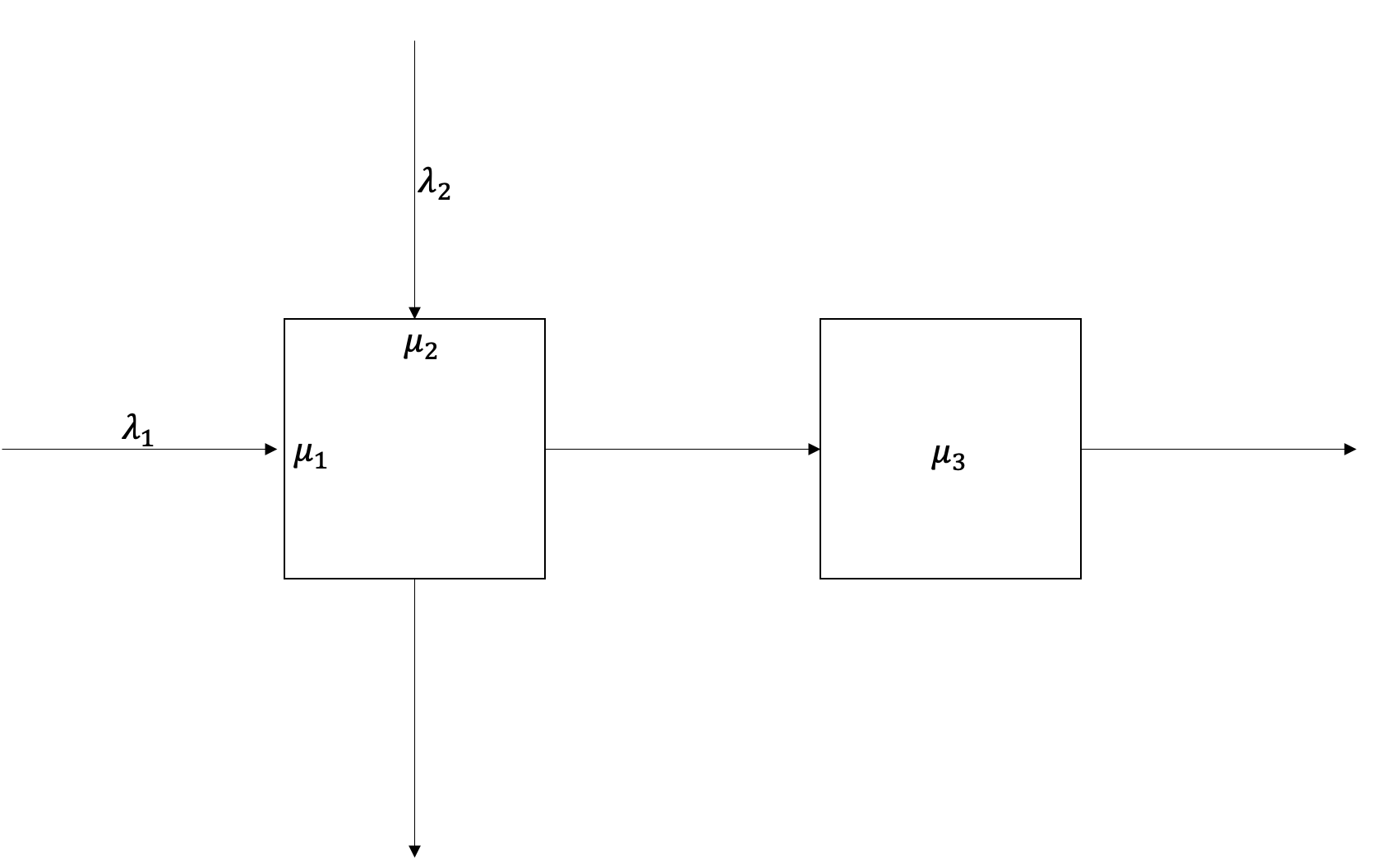
Figure 1: Criss-cross network.

Conditions	$\bm{u}^{*}(t)$
$\frac{x_{1}(t)}{x_{3}(t)}\geq\frac{c_{2}\mu_{1}}{c_{1}\mu_{1}-c_{3}\mu_{3}}\times\frac{\mu_{1}-\lambda_{1}}{\mu_{2}-\mu_{1}}$	$(1,0,1)$
$\frac{x_{1}(t)}{x_{3}(t)}\leq\frac{c_{2}\mu_{1}}{c_{1}\mu_{1}-c_{3}\mu_{3}}\times\frac{\mu_{1}-\lambda_{1}}{\mu_{2}-\mu_{1}}$	$(0,1,1)$

Table 1: Optimal policy for the criss-cross network when $\bm{x}(t)>\bm{0}$.

Figure 2 displays the decision tree learned by OCT-H, where each node contains the prediction made on that node. The decision tree that OCT-H learned predicts $\bm{u}^{*}(t)=(0,1,1)$ if $x_{1}(t)\leq 5.93x_{3}(t)+0.01$ and predicts $\bm{u}^{*}(t)=(1,0,1)$ if $x_{1}(t)\geq 5.93x_{3}(t)+0.01$. This closely resembles the optimal policy, exhibiting only minor numerical differences.

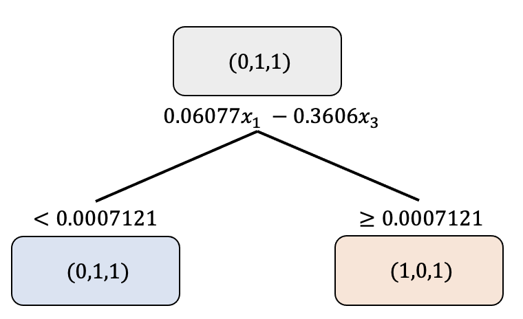
Figure 2: The decision tree learned by OCT-H for the criss-cross network.

The second example is the Rybko-Stolyar network studied in Rybko & Stolyar (1992). This network is composed of four classes and two servers. Server 1 processes Class 1 and 4, and Server 2 processes Class 2 and 3 jobs. Class 1 and 3 jobs take external arrivals. After Class 1 jobs are processed, they become Class 2 job and move to Server 2. After Class 3 jobs are processed, they become Class 4 jobs and move to Server 1. After Class 2 and 4 jobs are processed, they exit the system. Its graphical representation is given in Figure 3. We let $\bm{c}=\bm{e}$, $\lambda_{1}=\lambda_{3}=1$, $\mu_{1}=\mu_{3}=6$ and $\mu_{2}=\mu_{4}=1.5$. Under this set of parameters, the optimal policy is to prioritize Class 2 and 4 jobs unless either one of them is empty. If any one of them is empty, server splitting occurs. For this example, we train a single decision tree to learn the optimal policy that covers the entire state space. The parameters we used for Algorithm 1 are $N=1,t_{1}=0,\mathcal{A}=\{0.5,1.5\},\mathcal{P}=\{\mathcal{S}\}$ and $M=1000$.

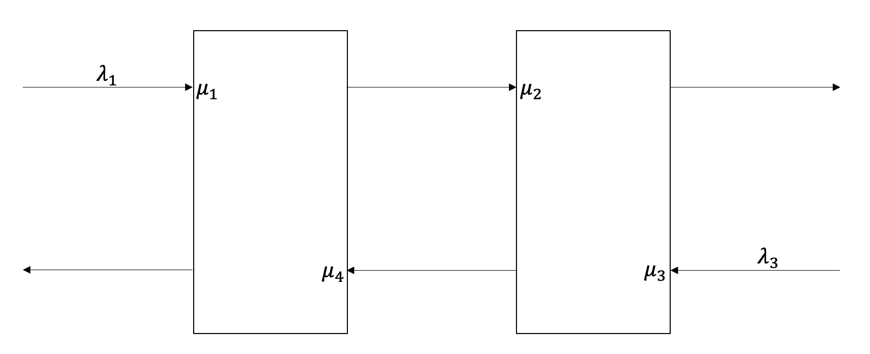
Figure 3: Rybko-Stolyar network.

Figure 4 displays the decision tree learned by OCT-H. Since decision trees are confined to use inequalities for node splits, we can observe that the condition $x_{i}=0$ for some $i\in[4]$ is learned as $x_{i}\leq\epsilon$ for a number $\epsilon$ with small absolute value. As the state vectors are always non-negative, these two conditions are effectively equivalent. Additionally, when both Class 2 and 4 are non-empty, the decision tree prioritizes them. When either one of them is empty, server splitting occurs. This policy aligns with the description provided earlier. To assess the quality of this policy when server splitting occurs, we generated a test set following the same procedure as the training set but with $M=200,\mathcal{A}=\{5\}$. The classification accuracy was $100\%,$ implying that OCT-H learned a high-quality policy that is empirically optimal.

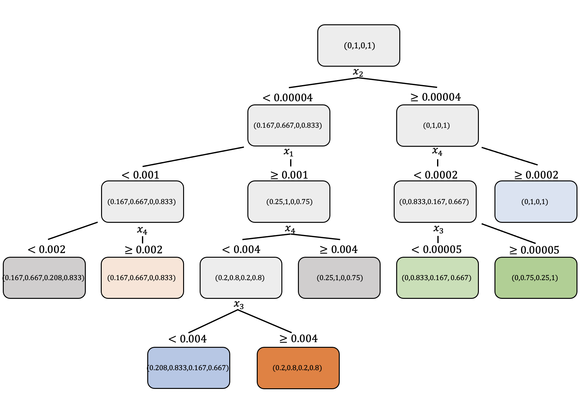
Figure 4: The decision tree learned by OCT-H for the Rybko-Stolyar network.

4 Computational Experiments

This section presents the findings of computational experiments conducted on MFQNETs with varying sizes. We analyze the accuracy of the policy learned by Algorithm 1 and compare its online application speed with that of the algorithm by Shindin et al. (2021). In addition, we provide insights on the optimal policy of MFQNET control problems by presenting some of the actual decision trees. We also apply OCT-H with sparsity on several MFQNET problems and analyze the impact of sparsity on the performance and the resulting decision tree. The networks in this section are taken from (Bertsimas et al., 2015) and (Shindin et al., 2021).

4.1 Experiment Setting

We consider a reentrant network with $m$ servers and $3m$ classes of jobs. Each Server $i\in[m]$ processes jobs of Classes $3(i-1)+1,3(i-1)+2$ and $3(i-1)+3$. Only Class 1 jobs take external arrivals with the arrival rate $\lambda_{1}$. Class $3(i-1)+1$ jobs become Class $3i+1$ until they become Class $3(m-1)+1$. After Class $3(m-1)+1$ jobs are processed, they change to Class 2 and enter Server 1. Class $3(i-1)+2$ jobs become Class $3i+2$ jobs until they become Class $3(m-1)+2$. After Class $3(m-1)+2$ jobs are processed, they change to Class 3 to enter Server 1. Class $3(i-1)+3$ jobs become $3i+3$ jobs, until they become Class $3m$ and exit the system after processed. We provide a graphical representation in Figure 5. The parameters $\bm{\lambda},\bm{\mu},\bm{c}$ are randomly generated using the software by Shindin et al. (2021).

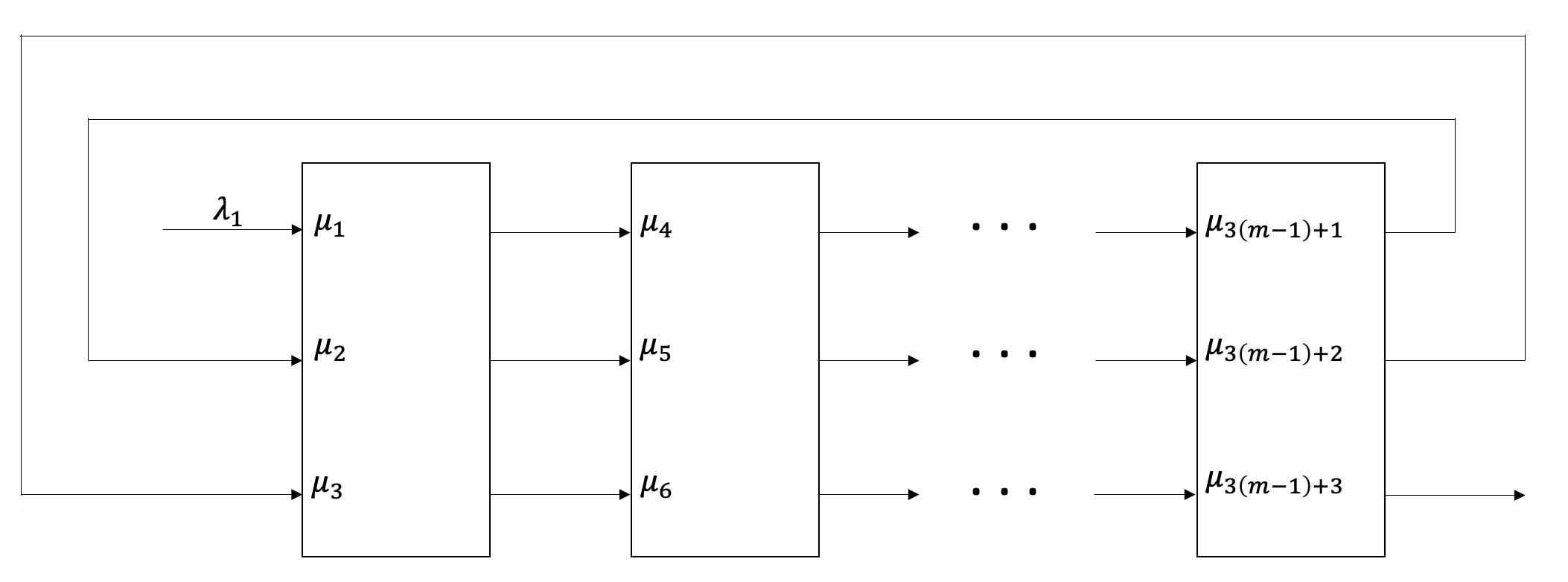
Figure 5: Reentrant network.

We test Algorithm 1 on the reentrant networks with varying $m$. We treat all $2^{3m}-1$ cases of non-zero entries separately. Using the formalism in Section 3.2, we let $\mathcal{P}=\big{\{}\{s_{1}\},\{s_{2}\},\dots,\{s_{2^{3m}-1}\}\big{\}}$. Instead of exhaustively demonstrating our approach on the entire cells of $\mathcal{P}$, we randomly choose three cells and learn the optimal policy for each cell. We always include the case where non of the classes are empty. After we fix some $s\in\mathcal{S}$, we generate a training set with $N=1,t_{1}=0,\mathcal{A}=\{0.5,0.75,5\}$ and $M=10000$. We generate a test set with $N=1,t_{1}=0,\mathcal{A}=\{10\}$ and $M=2000$. We report the classification accuracy of OCT-H on the test set. For each instance in the test set, we also measure the time it takes to solve the problem using the algorithm by Shindin et al. (2021), and divide it by the time it takes for the trained decision tree to make a prediction. We report the mean of the ratios rounded to the nearest integer as the relative speed-up of Algorithm 1.

Software for OCT-H is available at Interpretable AI (2023). We tune the maximum depth of the tree by grid searching over the list [3,5,10]. Public implementation of the algorithm by Shindin et al. (2021) is available at https://github.com/IBM/SCLPsolver. When we use this implementation, we set the zero entries in $\bm{\lambda}$ to a small number $10^{-6}$ instead of $0$, as we have observed that this results in better numerical stability. The experiments were executed on a MacBook Pro with 2.6 GHz Intel Core i7 CPU and 16GB of RAM, except for the training part. We trained decision trees on MIT Engaging Computing Cluster with Dell C6300, 2 socket Intel E5-2690v4 processor, 14 Cores per CPU and 128 GB RAM.

4.2 Speed and Accuracy

$m$	$|s|$	$|\{\bm{u}^{*}\}|$	Training Time (hours:minutes)	Speed-up	Classification Accuracy (%)
3	9	3	00:30	153	100
	7	3	00:38	196	100
	5	3	00:48	125	100
7	21	4	01:26	255	100
	9	4	00:34	151	100
	7	4	00:34	245	100
8	24	4	00:28	296	100
	12	4	00:44	278	100
	7	4	00:23	313	100
9	27	4	00:30	364	100
	24	2	00:33	360	100
	7	2	00:40	343	100
14	42	6	03:50	781	100
	36	6	04:34	790	100
	7	4	04:20	661	100
20	60	9	46:20	700	100
	30	9	44:10	599	100
	7	9	40:24	628	100
33	99	9	48:20	6014	100
	51	9	47:30	994	100
	45	9	42:20	982	100

Table 2: Experiment results for the reentrant network.

In Table 2, we report the results of numerical experiments, focusing on the speed and accuracy of Algorithm 1. In the second column, we report the number of non-zero entries of the state vector, denoted by $|s|$. In the third column, we report the number of distinct labels for the classification task, denoted by $|\{\bm{u}^{*}\}|$. In the rest of the columns we report $m$, the training time for OCT-H, the relative speed-up of Algorithm 1 and the out-of-sample classification error on the test set, rounded to the third decimal place.

Observations from Table 2

• Algorithm 1 achieves perfect accuracy regardless of the size of the network, the number of unique labels and the number of non-zero entries.

• The training time for OCT-H takes at most 48 hours in our experiment, suggesting that data generation and training might take hours to days in practice.

• Once a policy is learned, Algorithm 1 is significantly faster than the algorithm by Shindin et al. (2021), with a speed-up ranging from hundreds to thousands of times faster in our experiment. In general, this relative speed-up becomes even greater as the dimension of the state space gets higher.

• As the dimension of the state space gets higher, the number of distinct labels do not increase significantly. This observation suggests that even for high dimensional problems, the structure of the optimal policy might be simple enough to be learned by OCT-H with shallow decision trees.

4.3 Interpretability

We now provide the decision tree for a problem solved in Section 4.2 and develop insights on the structure of the learned policy. Although not all of the node splits have straightforward interpretations, we highlight a few splits that make intuitive sense.

Due to space concerns, we display the prediction targets in the tree figures as the list of job classes that are prioritized, rather than the optimal control vector $\bm{u}^{*}$ itself. The job classes that are prioritized receive effort 1, and the rest of the job classes receive effort 0. In addition, we assign a number to each node split and provide a separate table that contains information on the hyperplane for each split.

Furthermore, we introduce a vector ${\bm{c}}/{\bm{\mu}}$ that offers an interesting interpretation on the learned policy. This vector captures the relative cost of holding each job class in terms of their service rate. A higher value in this vector indicates that the corresponding job class poses a greater challenge to the fluid network controller.

In Figure 6, we provide the decision tree for the problem with $m=7$, confined to strictly positive state vectors ($|s|=21$). In Table 3, we provide the node split information associated with the decision tree. For this problem, the parameters rounded to the third decimal place are

$$\bm{\mu}=(0.143,0.253,0.002,0.287,0.169,0.278,0.22,0.11,0.207,0.216,0.299,0.004,0.185,0.205,$$

$$0.25,0.268,0.027,0.028,0.245,0.168,0.248),$$

$$\bm{c}=(0.705,0.235,0.972,0.968,0.719,0.107,1.484,1.395,0.493,0.746,1.584,1.512,0.07,0.892,$$

$$1.255,0.305,1.941,1.496,0.643,1.021,1.975).$$

After we compute $\bm{c}/\bm{\mu}$ and sort it in descending order, the resulting indices in the sorted order is

$$(3,12,17,18,8,21,7,20,11,15,1,14,5,10,4,19,9,16,2,6,13).$$

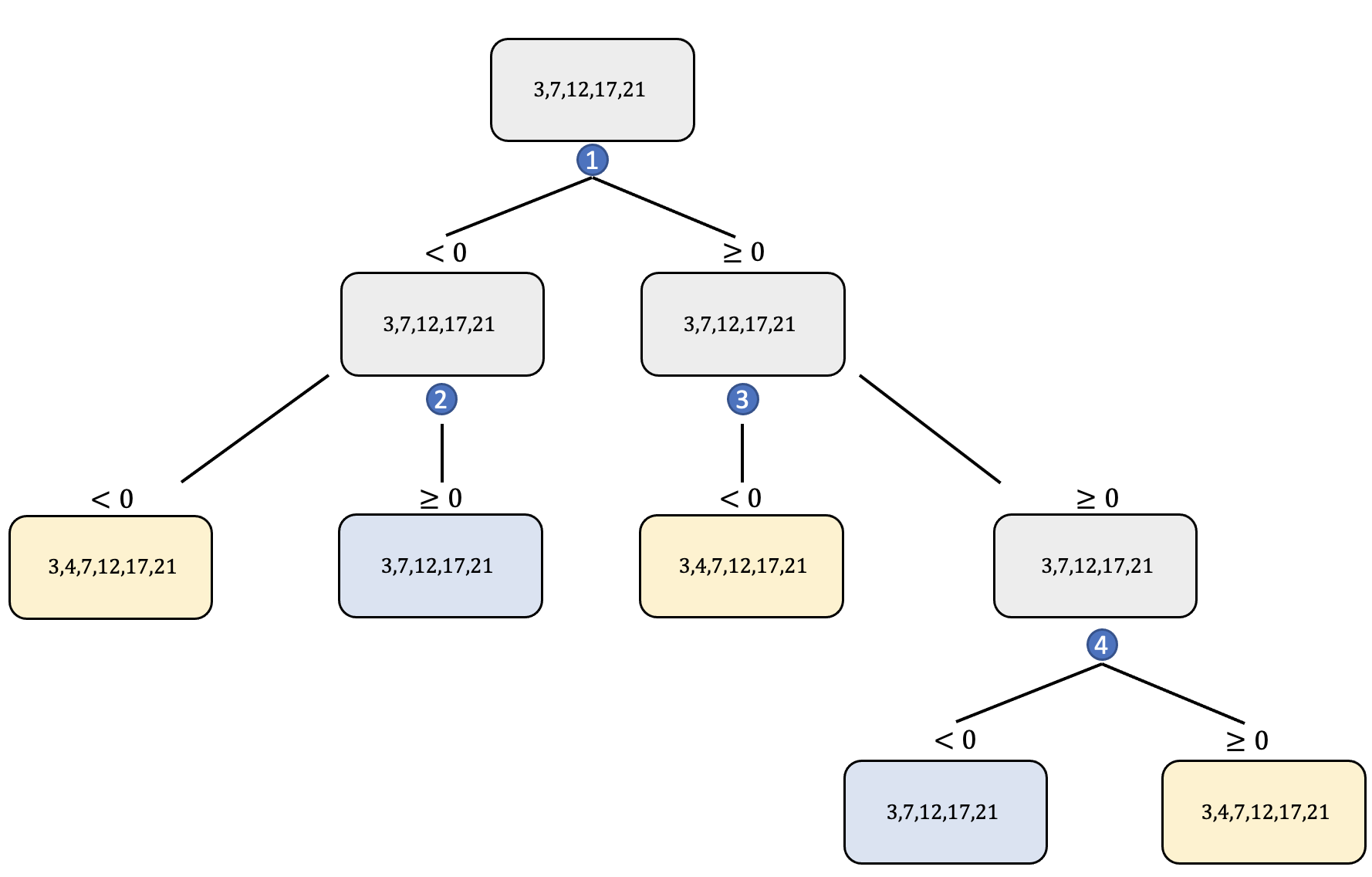
Figure 6: The decision tree learned by OCT-H for the reentrant network with $m=7$ and $|s|=21$.

Node split number	Hyperplane
1	$0.144x_{1}-0.002x_{4}+0.17x_{7}-0.05x_{10}-0.0005$
2	$-0.096x_{4}+1.036x_{7}$
3	$-732.7x_{1}-34.84x_{2}-5.311x_{3}-1989.5x_{4}+19.1x_{5}$
	$+14304.6x_{7}+4.175x_{8}+2939.7x_{10}+33.72x_{11}+62.25x_{12}$
	$-6.67x_{13}-12.42x_{14}+1.382x_{15}+8.84x_{16}-2.794x_{19}+12.92x_{20}$
4	$-2711.2x_{3}+0.5262x_{12}-0.0001$

Table 3: Node split information on the decision tree in Figure 6.

Observations from Figure 6

• Class 3,7,12,17,21 jobs are always prioritized, regardless of the node. These job classes are often the highest ranking classes within their respective server in terms of the value in the vector ${\bm{c}}/{\bm{\mu}}$. The only exception is Class 8, as Class 8 is not prioritized even though it is ranked the highest in its server. This observation implies that the learned policy for this network is to drain the “toughest" job classes from the system first.

• The only difference in the nodes is whether to process Class 4 jobs or idle Server 2. See split 1 and 2, for example. If $x_{4}$ is relatively large compared to a linear combination of $x_{1},x_{7},x_{10}$, and if $x_{4}$ is again relatively large compared to $x_{7}$, the decision is to process Class 4 jobs instead of idling Server 2. However, after traversing the left edge in split 1, if $x_{7}$ turns out to be too large compared to $x_{4}$, Class 4 jobs are not processed. A possible explanation is that as Class 4 jobs become Class 7 after processed, it might be beneficial to idle Server 2 in case there are too many Class 7 jobs waiting in the queue.

• See split 3. If we focus on the terms associated with $x_{4}$ and $x_{7}$, again the decision is to process Class 4 jobs if $x_{4}$ is relatively large compared to $x_{7}$. The same interpretation as above can be applied to this decision.

4.4 OCT-H with sparsity

In this experiment, we apply OCT-H with sparsity instead of OCT-H in Algorithm 1 on a subset of the problems solved in Section 4.2. As mentioned in Section 2.3, OCT-H with sparsity often results in more interpretable decision trees compared to OCT-H. The purpose of this experiment is to analyze the price we have to pay in order to gain more interpretability. We vary the proportion of the total number of states allowed to be used for splits, denoted by sparsity parameter. We analyze how the sparsity parameter affects the training time and the classification accuracy on the test set. Table 5 provides the experiment results, where the same notations as Table 2 are used. We summarize our findings in the following.

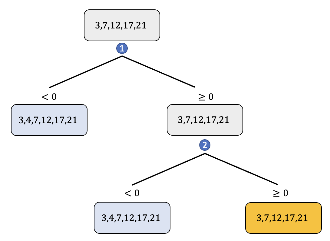
Figure 7: The decision tree learned by OCT-H with the sparsity parameter 0.25 for the reentrant network with $m=7$ and $|s|=21$.

Node split number	Hyperplane
1	$-0.316x_{4}+3.398x_{7}$
2	$-0.034x_{1}-0.103x_{4}+0.753x_{7}+0.152x_{10}+0.0003x_{11}$

Table 4: Node split information on the decision tree in Figure 7.

$m$	$|s|$	Sparsity Parameter	Training Time (hours:minutes)	Classification Accuracy (%)
7	21	0.5	00:48	99.8
		0.25	00:35	99.8
9	27	0.5	00:08	100
		0.25	00:07	100
14	42	0.5	02:52	98.3
		0.25	00:58	97
20	60	0.5	27:28	95.3
		0.25	14:20	94
33	99	0.5	26:51	94
		0.25	14:14	94

Table 5: Experiment results for the reentrant network using OCT-H with sparsity.

Observations from Table 5

• In general, classification accuracy slightly degrades as sparsity parameter gets smaller. However, classification accuracy never gets below 94% in our experiment, suggesting that OCT-H with sparsity can still learn high-quality policies.

• Training becomes faster as the sparsity parameter gets smaller. For the sparsity parameter 0.25, training can be around 4 times faster than OCT-H.

We provide the decision tree for the problem with $m=7,s=21$ and the sparsity parameter 0.25 in Figure 7. We compare this tree with the tree in Figure 6, which is learned by OCT-H on the same problem. Note that OCT-H with sparsity achieves 99.8 % accuracy on this problem, which is only 0.2 % decrease compared to OCT-H. Node split information is given in Table 4.

Observations from Figure 7

• The states used for the splits are a strict subset of the states used for the splits in Figure 6.

• The learned policy is also qualitatively similar to the policy learned with OCT-H. For example, in split 1, if $x_{4}$ is relatively large compared to $x_{7}$, the decision is to process Class 4 jobs. In split 2, if we focus on the terms associated with $x_{4}$ and $x_{7}$, again the decision is to process Class 4 jobs if $x_{4}$ is relatively large compared to $x_{7}$. Else, we idle Server 2 so that the queue on Class 7 jobs do not increase.

5 Conclusions

We presented an approach to solve MFQNET control problems using OCT-H. We proved that MFQNET control problems have threshold type optimal policies, and the threshold curves are hyperplanes passing through the origin. Based on this result, we developed an algorithm to use OCT-H to learn the optimal policy of MFQNET control problems. Computational experiments demonstrate that OCT-H can learn empirically optimal policies of MFQNET control problems with varying sizes. Once the policy is learned, we can solve MFQNET control problems considerably faster than the state-of-the-art algorithm by Shindin et al. (2021). Furthermore, we demonstrated that the simple decision tree structure enables us to develop insights on large dimensional MFQNET control problems.

References

- Alvarez et al. (2017) Alvarez, A. M., Louveaux, Q., & Wehenkel, L. (2017). A machine learning-based approximation of strong branching. INFORMS Journal on Computing, 29, 185–195.
- Anderson et al. (1983) Anderson, E. J., Nash, P., & Perold, A. F. (1983). Some properties of a class of continuous linear programs. SIAM Journal on Control and Optimization, 21, 758–765.
- Avram (1997) Avram, F. (1997). Optimal control of fluid limits of queueing networks and stochasticity corrections. Lecture in Applied Mathematics-American Mathematical Society, 33, 1–36.
- Avram et al. (1995) Avram, F., Bertsimas, D., & Ricard, M. (1995). An optimal control approach to optimization of multiclas queueing network. IMA volumes in Mathematics and its Applications, 71, 199–234.
- Balcan et al. (2020) Balcan, M.-F., Sandholm, T., & Vitercik, E. (2020). Learning to optimize computational resources: Frugal training with generalization guarantees. In The Thirty-Fourth AAAI Conference on Artificial Intelligence, AAAI 2020, The Thirty-Second Innovative Applications of Artificial Intelligence Conference, IAAI 2020, The Tenth AAAI Symposium on Educational Advances in Artificial Intelligence, EAAI 2020, New York, NY, USA, February 7-12, 2020 (pp. 3227–3234). AAAI Press.
- Bampou & Kuhn (2012) Bampou, D., & Kuhn, D. (2012). Polynomial approximations for continuous linear programs. SIAM Journal on Optimization, 22, 628–648.
- Bäuerle (2001) Bäuerle, N. (2001). Discounted stochastic fluid programs. Mathematics of Operations Research, 26, 401–420.
- Bäuerle (2002) Bäuerle, N. (2002). Optimal control of queueing networks: an approach via fluid models. Advances in Applied Probability, 34, 313–328. doi:10.1239/aap/1025131220.
- Bertsimas & Dunn (2017) Bertsimas, D., & Dunn, J. (2017). Optimal classification trees. Machine Learning, 106, 1039–1082.
- Bertsimas & Dunn (2019) Bertsimas, D., & Dunn, J. (2019). Machine learning under a modern optimization lens. Dynamic Ideas.
- Bertsimas & Gamarnik (2022) Bertsimas, D., & Gamarnik, D. (2022). Queueing Theory: Classical and Modern Methods. Dynamic Ideas.
- Bertsimas & Kim (2023a) Bertsimas, D., & Kim, C. (2023a). A machine learning approach to two-stage adaptive robust optimization. European Journal of Operations Research, . Submitted.
- Bertsimas & Kim (2023b) Bertsimas, D., & Kim, C. (2023b). A prescriptive machine learning approach to mixed integer convex optimization. INFORMS Journal on Computing, .
- Bertsimas et al. (2015) Bertsimas, D., Nasrabadi, E., & Paschalidis, I. C. (2015). Robust fluid processing networks. IEEE Transactions on Automatic Control, 60, 715–728.
- Bertsimas & Sethuraman (2002) Bertsimas, D., & Sethuraman, J. (2002). From fluid relaxations to practical algorithms for job shop scheduling: the makespan objective. Mathematical Programming, 92, 61–102.
- Bertsimas & Stellato (2021) Bertsimas, D., & Stellato, B. (2021). The voice of optimization. Machine Learning, 110, 249–277.
- Bertsimas & Stellato (2022) Bertsimas, D., & Stellato, B. (2022). Online mixed-integer optimization in milliseconds. INFORMS Journal on Computing, . Appeared online.
- Brieman et al. (1984) Brieman, L., Friedman, J., Stone, C. J., & Olshen, R. (1984). Classification and Regression Trees. Chapman and Hall/CRC.
- Cauligi et al. (2022) Cauligi, A., Culbertson, P., Schmerling, E., Schwager, M., Stellato, B., & Pavone, M. (2022). CoCo: Online mixed-integer control via supervised learning. IEEE Robotics and Automation Letters, 7, 1447–1454.
- Cochran & Roche (2009) Cochran, J. K., & Roche, K. T. (2009). A multi-class queuing network analysis methodology for improving hospital emergency department performance. Computers & Operations Research, 36, 1497–1512.
- Dai (1995) Dai, J. (1995). On positive harris recurrence of multiclass queueing networks: A unified approach via fluid limit models. The Annals of Applied Probability, 5, 49–77.
- Dai & Gluzman (2022) Dai, J., & Gluzman, M. (2022). Queueing network controls via deep reinforcement learning. Stochastic Systems, 12, 30–67.
- Dai & Weiss (2002) Dai, J., & Weiss, G. (2002). A fluid heuristic for minimizing makespan in job-shops. Operations Research, 50, 692–707.
- Dumas (1999) Dumas, V. (1999). Diverging paths in fifo fluid networks. IEEE Transactions on Automatic Control, 44, 191–194.
- Fleischer & Sethuraman (2005) Fleischer, L., & Sethuraman, J. (2005). Efficient algorithms for separated continuous linear programs: The multicommodity flow problem with holding costs and extensions. Mathematics of Operations Research, 30, 916–938.
- Gamarnik & Hasenbein (2005) Gamarnik, D., & Hasenbein, J. J. (2005). Instability in stochastic and fluid queueing networks. The Annals of Applied Probability, 15, 1652–1690.
- Harrison & Wein (1990) Harrison, J. M., & Wein, L. M. (1990). Scheduling networks of queues: Heavy traffic analysis of a two-station closed network. Operations Research, 38, 1052–1064.
- Hartl et al. (1995) Hartl, R. F., Sethi, S. P., & Vickson, R. G. (1995). A survey of the maximum principles for optimal control problems with state constraints. SIAM Review, 37, 181–218.
- Hutter et al. (2011) Hutter, F., Hoos, H. H., & Leyton-Brown, K. (2011). Sequential model-based optimization for general algorithm configuration. In Proceedings of the 5th International Conference on Learning and Intelligent Optimization LION’05 (p. 507–523). Berlin, Heidelberg.
- Interpretable AI (2023) Interpretable AI, L. (2023). Interpretable AI documentation. URL: https://www.interpretable.ai.
- Khalil et al. (2016) Khalil, E. B., Bodic, P. L., Song, L., Nemhauser, G., & Dilkina, B. (2016). Learning to branch in mixed integer programming. In Proceedings of the Thirtieth AAAI Conference on Artificial Intelligence AAAI’16 (p. 724–731). AAAI Press.
- Kumar (1993) Kumar, P. R. (1993). Re-entrant lines. Queueing Systems, 13, 87–110.
- Liu et al. (2019) Liu, B., Xie, Q., & Modiano, E. (2019). Reinforcement learning for optimal control of queueing systems. In 2019 57th Annual Allerton Conference on Communication, Control, and Computing (Allerton) (pp. 663–670).
- Luo & Bertsimas (1998) Luo, X., & Bertsimas, D. (1998). A new algorithm for state-constrained separated continuous linear programs. SIAM Journal on Control and Optimization, 37, 177–210.
- Maglaras (1999) Maglaras, C. (1999). Dynamic scheduling in multiclass queueing networks: Stability under discrete-review policies. Queueing Systems, 31, 171–206.
- Maglaras (2000) Maglaras, C. (2000). Discrete-review policies for scheduling stochastic networks: trajectory tracking and fluid-scale asymptotic optimality. The Annals of Applied Probability, 10, 897 – 929.
- Meyn (2007) Meyn, S. (2007). Control Techniques for Complex Networks. (1st ed.). USA: Cambridge University Press.
- Meyn (1995) Meyn, S. P. (1995). Transience of multiclass queueing networks via fluid limit models. The Annals of Applied Probability, 5, 946–957.
- Pontryagin et al. (1963) Pontryagin, L. S., Boltyanskii, V. G., Gamkrelidze, R. V., & Mishechenko, E. F. (1963). The mathematical theory of optimal processes. viii + 360 s. new york/london 1962. john wiley & sons. preis 90/–. Zamm-zeitschrift Fur Angewandte Mathematik Und Mechanik, 43, 514–515.
- Pullan (1993) Pullan, M. C. (1993). An algorithm for a class of continuous linear programs. SIAM Journal on Control and Optimization, 31, 1558–1577.
- Pullan (1995) Pullan, M. C. (1995). Forms of optimal solutions for separated continuous linear programs. SIAM Journal on Control and Optimization, 33, 1952–1977.
- Pullan (1996) Pullan, M. C. (1996). A duality theory for separated continuous linear programs. SIAM Journal on Control and Optimization, 34, 931–965.
- Pullan (1997) Pullan, M. C. (1997). Existence and duality theory for separated continuous linear programs. Mathematical Modelling of Systems, 3, 219–245.
- Pullan (2002) Pullan, M. C. (2002). An extended algorithm for separated continuous linear programs. Mathematical Programming, 93, 415–451.
- Raeis et al. (2021) Raeis, M., Tizghadam, A., & Leon-Garcia, A. (2021). Queue-learning: A reinforcement learning approach for providing quality of service. In AAAI Conference on Artificial Intelligence.
- Rybko & Stolyar (1992) Rybko, A., & Stolyar, A. (1992). On the ergodicity of stochastic processes describing functioning of open queueing networks. Problemy Peredachi Informatsii, 28, 3–26.
- Sethi (2019) Sethi, S. P. (2019). Optimal Control Theory. Springer.
- Shindin et al. (2021) Shindin, E., Masin, M., Weiss, G., & Zadorojniy, A. (2021). Revised sclp-simplex algorithm with application to large-scale fluid processing networks. In 2021 60th IEEE Conference on Decision and Control (CDC) (pp. 3863–3868).
- Srikant & Ying (2014) Srikant, R., & Ying, L. (2014). Communication Networks: An Optimization, Control and Stochastic Networks Perspective. USA: Cambridge University Press.
- Stolyar (1995) Stolyar, A. L. (1995). On the stability of multiclass queueing networks: A relaxed sufficient condition via limiting fluid processes. Markov Processes And Related Fields, 1, 491–512.
- Weiss (2008) Weiss, G. (2008). A simplex based algorithm to solve separated continuous linear programs. Mathematical Programming, 115, 151–198.