Linear magnetic susceptibility of anisotropic superconductors of cuboidal shape

Abstract

A simplified model of anisotropic magnetic susceptibility in the Meissner-London vortex-free state of cuboidal superconducting samples is presented. Using this model, precision measurements of the magnetic response in three perpendicular directions of a magnetic field with respect to primary crystal axes, can be used to extract the components of the London penetration depth, thus enabling the evaluation of the general superfluid density tensor, which is needed in the analysis of the superconducting gap structure.

I Introduction

Magnetic measurements are some of the most common ways to analyze magnetic and superconducting materials. While in the magnets, the response comes from atomic and spin magnetism, in superconductors, the magnetic response is distinctly different and non-local. It comes from the screening currents circulating at the scale of the entire sample.

The problem of extracting the components of the superfluid density tensor became crucial with the discovery of highly anisotropic high$-T_{c}$ cuprates [1, 2]. It was realized that the response to an applied magnetic field involves at least two components of the London penetration depth [3, 4, 5, 6, 7, 8]. If the crystallographic axes are not aligned along the principal sample faces, the problem is hard to tackle. Therefore, similarly to prior works, we will assume that crystal lattice unit cell axes are aligned along the normal directions to the sample facets, which is assumed to be a rectangular parallelepiped, as shown in Fig.1. One way to extract the individual components of the London penetration depth is to use optical methods measuring by measurement of the infrared reflectances with polarization along the $a$, $b$, and $c-$axes [3]. However, lower frequency and even DC measurements are needed and there one has to rely on the global response of the entire sample and in this case measured quantity depends on at least two components of screening current.

In order to extract separate components of the London penetration depth, $\lambda_{i}$, where $i=a,b,c$ it was suggested to use thin crystals and apply magnetic field along the flat faces to avoid demagnetizing effects and, in case of layered materials, minimize the contribution from the inter-plane currents described by the $c-$axis penetration depth, $\lambda_{c}$. One can double the contribution of this component by cutting the sample in half creating two new surfaces with $c-$axis currents. When such cut sample (both halves) is re-measured it is straightforward to use the results of both measurements to extract both components [6, 7]. This technique is especially useful in highly anisotropic materials. The same cutting (cleaving) method can be used for any other component [5]. In the most sensitive techniques, only the variation of the London penetration depth is measured precisely and determination of the absolute values, $\lambda_{i}\left(0\right)$, requires separate efforts [9, 5, 8]. Often, different methods are combined to obtain the final result [8, 5].

In this contribution I describe a self-contained method to estimate the components of the penetration depth measuring bulk thick samples. In fact a cube-shape sample will be ideal. It has the same demagnetizing factor of $N=0.39$ in three orthogonal directions (yes, the sum must be equal to 1 only in ellipsoids) [10] and the difference in three measured components along each axis is solely due to the anisotropy of the superfluid response.

We are interested in weak magnetic fields, much lower than the first critical field, $H_{c1}$, long before vortices begin entering the sample. The impossible-to-achieve Meissner state is established when the magnetic induction is zero everywhere in the sample. The realistic Meissner-London state allows some magnetic field in a thin layer called London penetration depth. In this situation, the magnetic response is linear and, in the semi-classical approach, is governed by the London equation [11, 12],

$$\mathbf{j}=-\mathbb{R}\mathbf{A}$$ (1)

that connects the supercurrent density vector, $\mathbf{j}$, and a vector potential, $\mathbf{A}$. The response tensor, $\mathbb{R}$, consists of two parts, diamagnetic and paramagnetic, and is determined by the superconducting gap and the parameters of the electronic band structure [11]. Some examples of using this theory for different superconducting order parameters can be found in Ref. [13]. Equation 1 takes a more familiar form when the London penetration depth is introduced,

$$\lambda_{ii}^{2}=\frac{m^{*}}{\mu_{0}n_{s}e^{2}}=\frac{1}{\mu_{0}\mathbb{R}_{ii}}$$ (2)

where $m^{*}$ is the effective electron mass and $n_{s}$ is the density of electrons in a superfluid fraction in a two-fluid model [14, 15, 16, 12]. Theoretically, it is possible to consider individual components of the supercurrent or, equivalently, the components of the London penetration depth separately, assuming infinite or semi-infinite samples. In practice, however, the samples are finite, and the response always contains different components.

II Anisotropic magnetic susceptibility

The total magnetic moment of an arbitrarily shaped magnetic sample is given by [10]:

$$\bm{m}=\int\left(\mu_{0}^{-1}\bm{B}\left(\bm{r}\right)-\bm{H}_{0}\right)dV$$ (3)

where $H_{0}$ is the applied magnetic field, and the integration is carried over the volume that completely encloses the sample. This equation is trivial in the infinite geometries (without demagnetization effects), but for arbitrary samples, requires a rigorous derivation from the general equation for the magnetic moment via the integration of shielding currents, $\bm{m}=\int\bm{r}\times\bm{j}(\bm{r})dV/2$ [10]. In fact, Eq.(3) includes the demagnetization effects and can be used to define the effective demagnetization factors [10]. Initial magnetic flux penetration into a $\lambda-$layer in a superconductor is linear in $\lambda/R\ll 1$. When penetrating flux sweeps about 1/3 of the sample dimension in the penetration direction, highly non-linear (hyperbolic) functions take over so that diverging with temperature $\lambda\left(T\right)/R$ results in zero magnetic susceptibility. For example, for an infinite slab of width $2w$, $\chi=(\lambda/w)\tanh(w/\lambda)-1$. However, when $\lambda/w$ ratio is small, $\tanh(w/\lambda)\approx 1$, and the magnetic susceptibility can be quite generally written as [17]:

$$\chi\left(1-N\right)=D\frac{\lambda}{R}-1$$ (4)

where $D$ is the dimensionality of the flux penetration, and $N$, is the demagnetizing factor in the direction of the applied magnetic field. In particular, $D=1$ for an infinite slab in a parallel magnetic field, $D=2$ for an infinite cylinder in a parallel field, and $D=3$ for a sphere). In typical sub-mm crystals, $R\sim 100$$\>\mu\mathrm{m}$  [17] and $\lambda\left(0\right)\sim 200$ nm, therefore $\lambda\left(0\right)/R\approx 2\times 10^{-3}$, a small number considering the total variation of $\chi$ from zero to $-1$. Moreover, this is applicable practically at all temperatures. To see that, we can estimate the temperature at which $\lambda$ doubles. Using well-known approximation, $\lambda\left(t\right)=\lambda_{0}/\sqrt{1-t^{2}}$ [13] ($t=T/T_{c}$ - reduced temperature), we estimate that the penetration depth doubles at $t=\sqrt{3}/2\approx 0.87$, which is practically the entire temperature range.

Linear approximation, Eq.4, means that we can calculate magnetic susceptibility as the ratio of the shielded volume to the total volume. Owing to the exponential attenuation of the magnetic field from the surface, one can roughly assume a complete field penetration into the layer of depth $\lambda$ and no magnetic field at all beyond that. Then, the volume penetrated by the magnetic flux is determined by the corresponding components of the London penetration depth, as shown in Fig.1.

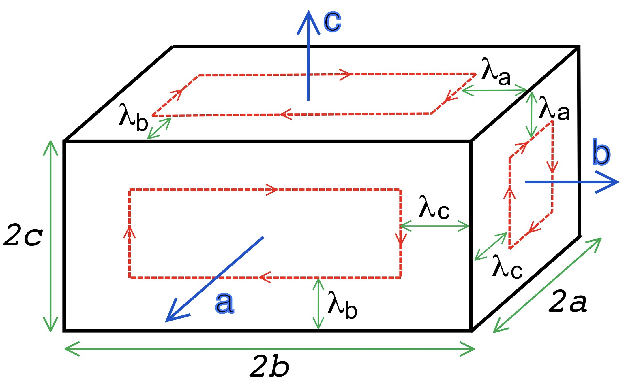
Figure 1: The definitions of symbols and directions in a cuboidal sample of size $2a\times 2b\times 2c$ showing different components of the London penetration depths. Directions of screening currents flow are shown by loops with arrows.

We need to define the components of the current density and the London penetration depth with respect to crystal axes. Consider a cuboid-shaped crystal of size $2a\times 2b\times 2c$. The vectors $\mathbf{a},\mathbf{b}$ and $\mathbf{c}$ point along the corresponding lengths as shown in Fig.1. When a magnetic field is directed along the $\mathbf{c}-$axis, screening currents flow in the $\mathbf{ab}-$plane. Current flowing along the $a-$side is attenuated on the length $\lambda_{a}$, whereas current flowing along the $b-$side by length $\lambda_{b}$. The gradient of the magnetic induction is perpendicular to the local direction of the current flow.

To obtain three unknown components of the London penetration depth one needs three components of magnetic susceptibility. Assuming that sample crystallographic directions are parallel to the sample sides, magnetic susceptibility needs to be measured in three principal directions, so that, for example, $\chi_{a}$ is magnetic susceptibility measured with a magnetic field applied along the $\mathbf{a}-$axis. For the analysis, it is crucially important to obtain properly normalized magnetic susceptibilities so that they include (direction-dependent) demagnetization correction, $\left(1-N\right),$ Using well-knowsee Eq.4. For example, we should have $\chi_{a}=-1$ when $\lambda_{c}=\lambda_{b}=0$ (ideal shielding). The practical experimental procedure depends on the measurement technique and measured quantity.

In the case of a DC magnetometry (Quantum Design MPMS, VSM, extraction magnetometer, Faraday balance, etc.), one can take the value of the magnetic moment at the lowest temperature and use it for normalization. For example, if a total magnetic moment, $m(T)$, is measured, then the normalized magnetic susceptibility is given my $\chi(T)=m(T)/|m_{0}|$, where the denominator is the theoretical magnetic moment of a perfect diamagnetic sample of the same shape, $m_{0}=-VH_{0}/(1-N)$, $V$ is sample volume and $H_{0}$ is the applied magnetic field. The normalization is performed assuming $m_{0}\approx m\left(T_{min}\right)$. Unfortunately, insufficient sensitivity, limited dynamic range, and omnipresent noise make it practically impossible to use DC magnetometry to determine the London penetration depth.

The biggest problem is that there is no true reference point, ideal diamagnetic response (i.e., a pure Meissner state), so the measurements are always performed with finite $\lambda(T)$, and one does not know what the signal would be with $\lambda=0$. Usually, only the variation of the London penetration depth with temperature is measured since it contains information about low-energy quasiparticles, hence the order parameter structure. For example, the rate of change is about 5 Å/K in YBCO, and 20 Å/K in BSCCO [3, 9, 8].

Let us take a superconducting ball of radius $R$. Its magnetic susceptibility in the pure Meissner state is $\chi=-\left(3/2\right)V=-2\pi R^{3}$, where $3/2=1/(1-1/3)$ prefactor is the demagnetization correction. Suppose we would like to detect the 5 Å  change of $\Delta\lambda\left(T\right)$ warming the sample by 1 K from the base temperature. The corresponding volume change in the ball is $4\pi R^{2}\Delta\lambda$. Therefore, we need to resolve the change of magnetic susceptibility, $4\pi R^{2}\Delta\lambda/2\pi R^{3}=2\Delta\lambda/R$. For a mm-sized crystal, we have for YBCO, $2\Delta\lambda/R\approx 10^{-6}$. The total magnetic moment of 1 mm ball is $m=-2\pi R^{3}H\approx-6\times 10^{-3}H$ emu, where magnetic field is in Oe. Therefore, one needs to detect a change in the magnetic moment of $\Delta m\approx 6\times 10^{-9}H$ emu. Here quoted sensitivity of the magnetometers mentioned above is $10^{-6}\;\text{emu}$. Therefore, with the excitation fields less than 10 Oe (usually much less), the required sensitivity of better than $6\times 10^{-8}$ emu is far beyond these instruments capabilities. Note that, ideally, we would want to resolve at least ten points in that 1 K interval. Then the resolution needs to be 10 time better. Of course, the magnetic moment is larger in higher fields, but one needs to worry about vortices at some point. Of course, this reasoning only applies to commercial systems measuring total magnetic moment of a sample.

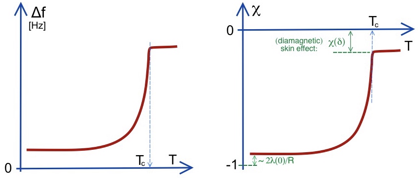
Figure 2: (left panel) Schematics of the measured signal, shown as the resonant frequency shift in the case of the frequency-domain susceptometry; (right panel) calibrated effective susceptibility. The deviations from the ideal behavior are associated with the finite London penetration depth at low temperatures and skin depth near $T_{c}$.

In the case of frequency-domain AC susceptibility measurements, such as tunnel-diode resonator (TDR) [18, 19, 13, 20], microwave cavity perturbation [21, 22, 23] or even amplitude-domain conventional AC susceptibility [24, 25], sufficient sensitivity and dynamic range can be achieved (although this requires a significant effort) for precision measurements of $\lambda(T)$. However, one can no longer take the signal difference from above $T_{c}$ to the lowest temperature because of the screening of the applied AC fields due to the normal skin effect. This is shown schematically in Fig.2 where the left panel shows typical resonant frequency variation upon sweeping temperature through $T_{c}$. The calibrated magnetic susceptibility needed for the analysis is depicted in the right panel. To determine the total screening, one can estimate the normal-state screening from the independent resistivity measurements through $T_{c}$. This is not the most precise approach because it involves sample-dependent calibration factors. Alternatively, the measurement device could allow for the physical extraction of the sample from the sensing coil in situ. This requires a substantial modification of the experimental setup, but once built, it gives the ability to calibrate every measured sample and automatically includes the demagnetization correction. This is implemented, for example, in our tunnel-diode resonators [20, 13, 19]. At low temperatures, the deviation from perfect screening, $2\lambda\left(0\right)/R\approx 4\times 10^{-3}$, is a small number.

III London penetration depth

Assuming that we have all three components of the normalized magnetic susceptibility, it is convenient to construct a vector of “normalized penetrated volumes”,

$$\bm{X}=\left(1+\chi_{a}\left(T\right),1+\chi_{b}\left(T\right),1+\chi_{c}\left(T\right)\right)$$ (5)

whose components vary from $1$ in case of a complete penetration ($\chi_{i}=0$) to $0$ in case of a complete screening ($\chi_{i}=-1$). For example, for $\mathbf{H}||\mathbf{c}$, the normalized penetrated volume is:

$$\chi_{c}=\frac{(2c)(2a)(2\lambda_{a})+(2c)(2b)(2\lambda_{b})}{V}=\frac{\lambda_{a}}{b}+\frac{\lambda_{b}}{a}$$ (6)

where sample volume $V=(2a)(2b)(2c)=8abc$. Doing the same for other two orientations, we obtain:

$$\bm{X}=\bm{L}\cdot\bm{\Lambda}$$ (7)

where the London penetration depth vector $\bm{\Lambda}=\left(\lambda_{a},\lambda_{b},\lambda_{c}\right)$ and the coupling London matrix is:

$$\bm{L}=\left(\begin{array}[]{ccc}0&\frac{1}{c}&\frac{1}{b}\\ \frac{1}{c}&0&\frac{1}{a}\\ \frac{1}{b}&\frac{1}{a}&0\end{array}\right)$$ (8)

The solution of this vector equation is,

$$\bm{\Lambda}=\bm{L}^{-1}\cdot\bm{X}$$ (9)

where the inverse of the London matrix is given by:

$$\bm{L}^{-1}\bm{=}\left(\begin{array}[]{ccc}-\frac{bc}{a}&c&b\\ c&-\frac{ac}{b}&a\\ b&a&-\frac{ab}{c}\end{array}\right)$$ (10)

The resulting solution written in components is:

$$\left\{\begin{array}[]{l}2\lambda_{a}=-\frac{bc}{a}\left(1+\chi_{a}\right)+c\left(1+\chi_{b}\right)+b\left(1+\chi_{c}\right)\\ 2\lambda_{b}=c\left(1+\chi_{a}\right)-\frac{ac}{b}\left(1+\chi_{b}\right)+a\left(1+\chi_{c}\right)\\ 2\lambda_{c}=b\left(1+\chi_{a}\right)+a\left(1+\chi_{b}\right)-\frac{ab}{c}\left(1+\chi_{c}\right)\end{array}\right.$$ (11)

This allows evaluating three principal components of the London penetration depths from three independent magnetic susceptibility measurements. Indeed, it is hard to find perfect samples with ideal geometry, so errors in the amplitudes are inevitable. However, this procedure may help identify some non-trivial temperature dependencies of the penetration depth, distinguish nodal from nodeless states, or correlate with resistivity anisotropies in search of nematic states. These estimates may be useful when other parameters are also available, for example, specific heat, resistivity, and upper critical field, which are tied together by thermodynamic Rutgers relations [26, 27].

IV tetragonal crystals

The general relation, Eq.11, is simplified if one considers a quite typical for superconductors case of tetragonal (or close to tetragonal) symmetry of the crystal lattice. High$-T_{c}$ cuprates and iron-based superconductors are notable examples. In this case, there are two principal values of the London penetration depth, in plane, $\lambda_{a}=\lambda_{b}=\lambda_{ab}$, and out of plane, $\lambda_{c}.$ Note, however, that the sample still has three different sides, $a,b,c$. This means that all three components of the magnetic susceptibility will be different. In this case Eq.11 is simplified as:

$$\left\{\begin{array}[]{l}\lambda_{ab}=\frac{ab}{a+b}\left(1+\chi_{c}\right)\\ \lambda_{c}=b\left(1+\chi_{a}\right)-\frac{ab^{2}}{c\left(a+b\right)}\left(1+\chi_{c}\right)\\ ....=a\left(1+\chi_{b}\right)-\frac{ba^{2}}{c\left(a+b\right)}\left(1+\chi_{c}\right)\\ ....=\frac{ab}{b-a}\left(\chi_{b}-\chi_{a}\right)\end{array}\right.$$ (12)

These are useful formulas as they show that in order to evaluate the in-plane London penetration depth one needs to measure only $\chi_{c}$ which is what most experimentalists do. To obtain the $c-$axis penetration depth one needs to measure perpendicular components $\chi_{a}$ and/or $\chi_{b}$. Having both will improve the accuracy of the estimate.