Scalable solution to crossed random effects model with random slopes

The crossed random effects model is widely used, finding applications in various fields such as longitudinal studies, e-commerce, and recommender systems, among others. However, these models encounter scalability challenges, as the computational time for standard algorithms grows superlinearly with the number $N$ of observations in the data set, commonly $\Omega(N^{3/2})$ or worse. Recent work has developed scalable methods for crossed random effects in linear models and some generalized linear models, but those works only allow for random intercepts. In this paper we devise scalable algorithms for models that include random slopes. This problem brings a substantial difficulty in estimating the random effect covariance matrices in a scalable way. We address that issue by using a variational EM algorithm. In simulations, we see that the proposed method is faster than standard methods. It is also more efficient than ordinary least squares which also has a problem of greatly underestimating the sampling uncertainty in parameter estimates. We illustrate the new method on a large dataset (five million observations) from the online retailer Stitch Fix.

1 Introduction

In the era of Over The Top (OTT) platforms like Netflix, where customer acquisition is booming and a vast array of titles are hosted, the need for computationally efficient recommender systems has become crucial. In such scenarios, it is common for different clients to rate varying numbers of items, which gives a haphazard missingness pattern. We deal with one such problem where $R$ clients rate $C$ items, and it is usually the case that only $N\ll R\times C$ of the ratings are observed. Moreover, we consider a situation where we have access to various characteristics of each (item, client) pair, in addition to the client’s rating of the item. For instance, information such as the client’s age, gender, and purchase history can be combined with features of the item such as material and style for clothing or genre, language and duration for online content.

A concrete example of our motivating data sets comes from the online clothing retailer Stitch Fix. Quoting from Ghosh et al., 2022b :

Stitch Fix is an online personal styling service. One of their business models involves sending customers a sample of clothing items. The customer may keep and purchase any of those items and return the others. They have provided us with some of their client ratings data. That data was anonymized, void of personally identifying information, and as a sample it does not reflect their total numbers of clients or items at the time they provided it. It is also from 2015. While it does not describe their current business, it is a valuable data set for illustrative purposes.

We will present results using that data later, and we use the problem setup throughout this paper to explain the choices we make.

Our motivating scenario is to model clients’ ratings of items. To represent the rating provided by client $i$ for item $j$, we use the notation $Y_{ij}$, while the covariate information for the specific client-item pair $(i,j)$ is denoted as $x_{ij}$. In such settings, ordinary least squares is not advisable as the ratings are not independent. Instead, we expect some positive correlation between ratings by different clients on the same item, because some items are simply more popular than others in ways that cannot always be attributed to $x_{ij}$. We can similarly expect some positive correlation between ratings by one client on different items, because clients can vary in how strict they are. To account for these covariance structures, crossed random effects models are employed. These models are designed to capture the dependencies present in the ratings provided by the same client or for the same item.

One notable drawback of crossed random effects models is their limited scalability. As the dataset grows in size, the computational burden associated with fitting crossed random effects models becomes challenging and inefficient.  Ghosh et al., 2022a considered the crossed random-effects model with random intercept terms for clients and items, given by

$$Y_{ij}=\beta_{0}+a_{i}+b_{j}+x_{ij}^{\mathsf{T}}\beta+e_{ij},\hskip 14.22636pt\forall i\in\{1,\cdots,R\},\hskip 8.5359ptj\in\{1,\cdots,C\}.$$ (1)

Here, the random effects are $a_{i}\in\mathbb{R}$, $b_{j}\in\mathbb{R}$ and an error $e_{ij}\in\mathbb{R}$. The fixed effects are the regression parameters $\beta\in\mathbb{R}^{p}$ and the intercept $\beta_{0}\in\mathbb{R}$. They assume that $a_{i}\sim N(0,\sigma^{2}_{a})$ , $b_{j}\sim N(0,\sigma^{2}_{b}),$ and $e_{ij}\mathbin{\overset{i.i.d}{\kern 0.0pt\sim}}\mathbin{N}(0,\sigma^{2}_{e})$ are all independent. Under the above model,

$$\mathrm{Cov}(Y_{ij},Y_{ij^{\prime}})=\sigma^{2}_{a}\mbox{ and }\mathrm{Cov}(Y_{ij},Y_{i^{\prime}j})=\sigma^{2}_{b}\mbox{ for }i\neq i^{\prime},j\neq j^{\prime}.$$

Standard approaches involve employing crossed random effects models, which come with a computational burden proportionate to $(R+C)^{3}$, where $R$ and $C$ are the number of random effect levels. However, due to the relationship $RC\geq N$, this computational cost can be expressed as $\Omega(N^{3/2})$ (as detailed in Gao and Owen, (2020)). To address this limitation, Gao and Owen, (2020) introduced a moment-based method for estimating variance parameters in the intercept model (1) with a computational cost that is at most linear. More recently, Ghosh et al., 2022a developed a backfitting algorithm inspired by the work of Buja et al., (1989) that achieves linear computational cost in terms of $N$.

In contrast, the plain Gibbs sampler is not scalable, as it exhibits a computational cost of $\Omega(N^{3/2})$ (as shown in Gao and Owen, (2017)). Gao and Owen, (2017) also show that many other Bayesian approaches do not work well in crossed random effects settings. Recent work has shown that collapsed Gibbs sampling can be made to scale well in crossed random effects settings. See Papaspiliopoulos et al., (2020) and Ghosh and Zhong, (2021). Ghosh, (2022) presents an insightful connection between the convergence of backfitting and collapsed Gibbs. These works do not include the random slopes that we focus on here.

During the process of model fitting, Ghosh et al., 2022a also furnish estimates for $(a_{i})_{i=1}^{R}$ and $(b_{j})_{j=1}^{C}$, which can subsequently be used for making predictions on test data. This implies that the crossed random effects model can serve as a scalable recommender system. To assess its prediction accuracy, we measured the performance of the crossed random effects model with a random intercept on Stitch Fix data using a random train-test split. In comparison to ordinary least squares, which yielded an $R^{2}$ of 4.61 $\%$, the crossed random effects model (1) achieved an impressive $R^{2}$ of 18.42 $\%$. This significant improvement in $R^{2}$ shows the efficiency gains from crossed random effects models. As a result, we endeavor to develop an efficient and scalable implementation for crossed random effects, which includes random slopes.

$$Y_{ij}=\beta_{0}+a_{i}+b_{j}+x_{ij}^{\mathsf{T}}(\beta+\tilde{a}_{i}+\tilde{b}_{j})+e_{ij},\hskip 8.5359pt\forall i\in\{1,\cdots,R\},\hskip 8.5359ptj\in\{1,\cdots,C\},$$ (2)

where random effects $\tilde{a}_{i}\in\mathbb{R}^{p}$ and $\tilde{b}_{j}\in\mathbb{R}^{p}$ and an error $e_{ij}\in\mathbb{R}$. We assume that $\tilde{a}_{i}\sim N_{p}(0,\tilde{\Sigma}_{a})$ and $\tilde{b}_{j}\sim N_{p}(0,\tilde{\Sigma}_{b})$, with other terms having the same meaning. The crossed random effects model with random slopes helps us in capturing the variability of the effect size of covariates among different clients and items. Figure 1 provides a visual representation for model with random intercept and random slopes. The first plot represents a random effects model considering random intercept just for clients, second plot represents random effects model with random intercept as well as random slope for a continuous variable, “match” and the third plot represents a random effects model with random intercept and random slope for an indicator random variable “client edgy”.

Figure 1: In the left figure, we illustrate a model with random intercepts using continuous variable “match”. In the right figure, we illustrate a model with random intercepts as well as random slope for the continuous variable. The blue line represents the intercept and slope for fixed effects model in both the figures.

The model (2) could be rewritten in a compact form in the following way by applying the change of variables:-

$$Y_{ij}=x_{ij}^{\mathsf{T}}(\beta+a_{i}+b_{j})+e_{ij},\hskip 14.22636pt\forall i\in\{1,\cdots,R\},\hskip 8.5359ptj\in\{1,\cdots,C\}.$$ (3)

Here, the first coordinate of the covariate vector $x_{ij}\in\mathbb{R}^{p+1}$ is one, representing intercept terms as in (1). We assume that $a_{i}\sim N_{p+1}(0,\Sigma_{a})$ , $b_{j}\sim N_{p+1}(0,\Sigma_{b}),$ and $e_{ij}\mathbin{\overset{i.i.d}{\kern 0.0pt\sim}}\mathbin{N}(0,\sigma^{2}_{e})$ are all independent. Of course we can specify random effects for only a subset of the covariates, rather than for all of them. In our presentation, we have included random slopes for all the covariates for the sake of simplicity in notation.

The goal is to estimate the fixed effect $\beta$ and covariance parameters $\Sigma_{a}$, $\Sigma_{b}$, and $\sigma^{2}_{e}$. When $a_{i},b_{j}$ and $e_{ij}$ are gaussian, the GLS estimate of $\beta$ is also the maximum likelihood estimate (MLE). Thus, if the covariance matrix of the $N$-vector $Y$ is given by $\mathcal{V}\in\mathbb{R}^{N\times N}$ under the above model, the density of $Y$, hence the likelihood for ($\beta,\Sigma_{a},\Sigma_{b},\sigma^{2}_{e}$) will be given by

$$\frac{1}{\sqrt{(2\pi)^{N}|\mathcal{V}|}}\exp\left(-\frac{1}{2}(Y-X\beta)^{\mathsf{T}}\mathcal{V}^{-1}(Y-X\beta)\right)$$ (4)

Here, the vector $Y$ denotes all of the $Y_{ij}$ placed into a vector in $\mathbb{R}^{N}$ and $X$ denotes $x_{ij}$ stacked compatibly into a matrix in $\mathbb{R}^{N\times(p+1)}$. Under the above model, $(\ref{eq:random_slopes}$) and (4), the covariance matrix $\mathcal{V}$ of $Y$ is given by

$$\mathcal{V}=\left(X\Sigma_{a}X^{\mathsf{T}}\right)\bullet\left(Z_{a}Z_{a}^{\mathsf{T}}\right)+\left(X\Sigma_{b}X^{\mathsf{T}}\right)\bullet\left(Z_{b}Z_{b}^{\mathsf{T}}\right)+\sigma^{2}_{e}I_{N}$$ (5)

where $Z_{a}\in\{0,1\}^{N\times R}$ denotes the design matrix for clients, $Z_{b}\in\{0,1\}^{N\times C}$ denotes the design matrix for items and $A\bullet B$ denotes elementwise product of matrix $A$ and $B$. Let data point $t_{1}$ refer to the client-item pair $(i_{1},j_{1})$ and data point $t_{2}$ refer to the pair $(i_{2},j_{2})$, then

$$\mathcal{V}_{t_{1},t_{2}}=\begin{cases}0,&\text{if }i_{1}\neq i_{2}\text{ and }j_{1}\neq j_{2},\\ x_{i_{1}j}^{\mathsf{T}}\Sigma_{b}x_{i_{2}j},&\text{if }i_{1}\neq i_{2}\text{ and }j_{1}=j_{2}=j,\\ x_{ij_{1}}^{\mathsf{T}}\Sigma_{a}x_{ij_{2}},&\text{if }i_{1}=i_{2}=i\text{ and }j_{1}\neq j_{2},\\ x_{ij}^{\mathsf{T}}\Sigma_{a}x_{ij}^{\mathsf{T}}+x_{ij}^{\mathsf{T}}\Sigma_{b}x_{ij}+\sigma^{2}_{e},&\text{if }(i_{1},j_{1})=(i_{2},j_{2})=(i,j).\\ \end{cases}$$ (6)

Note: The term with $i_{1}=i_{2}=i$ and $j_{1}=j_{2}=j$, represent diagonal terms of the matrix, $\mathcal{V}$, i.e., variance of $y_{ij}$.
The covariance matrix is dense and not usefully structured, therefore obtaining $\hat{\beta}_{\mathrm{GLS}}$ using generalized least squares would be computationally expensive. We explore two potential methods to achieve the task.

• In our first approach, we provide consistent estimates of the covariance parameters using a method-of-moments approach illustrated in Section 3. We then proceed with estimating the fixed parameter given the covariance parameters using a backfitting approach, which is explained in Section 2. Both of the tasks can be accomplished in $\mathcal{O}(N)$ time.

The drawback of this first approach is that when the value of $p$ is large and the covariance matrices are non-diagonal, method of the moments may not produce accurate estimates for the covariance parameters.

• In our second approach, we maximize an approximation to the likelihood using “Variational EM” to estimate the fixed effects and covariance parameters simultaneously. It helps us in estimating covariance matrices precisely even when they are unstructured or $p$ is sufficiently large. Another advantage of this approach is its computational efficiency, with each step at most $\mathcal{O}(N)$.

The variational EM algorithm is closely related to the backfitting algorithm. Variational EM has been previously explored for fast and accurate estimation of non-nested binomial hierarchical models. Goplerud, (2021)

We speed up the convergence rate for both of the approaches, backfitting and variational EM using a technique referred to as “clubbing” discussed in 2.

1.1 Paper Outline

• In Section 2, we discuss the backfitting approach with and without clubbing.

• In Section 3, we discuss the estimation of covariance parameters using the method of moments in two scenarios: when the covariance matrices, $\Sigma_{a}$ and $\Sigma_{b}$ are diagonal, and when they are non-diagonal.

• In Section 4, we discuss the application of variational EM in estimating fixed as well as covariance parameters using an approximate maximum likelihood approach.

2 Estimation of the fixed parameter when covariance parameters are known

If the covariance parameters are known, the aim is to obtain $\hat{\beta}_{\mathrm{GLS}}$ in $\mathcal{O}(N)$ time. We know that the GLS estimate of $\beta$ is

$$\hat{\beta}_{\mathrm{GLS}}=\operatorname*{arg\,min}_{\beta}(Y-X\beta)^{\mathsf{T}}\mathcal{V}^{-1}(Y-X\beta)=(X^{\mathsf{T}}\mathcal{V}^{-1}X)^{-1}X^{\mathsf{T}}\mathcal{V}^{-1}Y$$ (7)

But, we couldn’t use the above formula directly to obtain $\hat{\beta}_{\mathrm{GLS}}$ as computing $\mathcal{V}^{-1}$ would take at least $\mathcal{O}(N^{3/2})$ time in the above setting. Therefore, it is important to suggest alternative approaches to obtain estimates for $\beta$. The theorem below helps us in setting up the motivation for the backfitting algorithm.

Theorem 1.

Consider the solutions to the following penalized least-squares problem

$$\min_{\beta,a_{i},b_{j}}\sum_{i=1}^{R}\sum_{j=1}^{C}\frac{z_{ij}(y_{ij}-x_{ij}^{\mathsf{T}}(\beta+a_{i}+b_{j}))^{2}}{\sigma^{2}_{e}}+\sum_{i=1}^{R}a_{i}^{\mathsf{T}}\Sigma^{-1}_{a}a_{i}+\sum_{j=1}^{C}b_{j}^{\mathsf{T}}\Sigma_{b}^{-1}b_{j}$$ (8)

Then $\hat{\beta}=\hat{\beta}_{\mathrm{GLS}}$ and the $\{\hat{a}_{i}\}_{i=1}^{R}$ and $\{\hat{b}_{j}\}_{j=1}^{C}$ are the best linear unbiased prediction (BLUP) estimates of the random effects.

Here $z_{ij}=1$ if the rating $Y_{ij}$ for the $(i,j)$ client-item pair is observed, and $z_{ij}=0$ otherwise.

The theorem was originally given by Robinson, (1991); we provide an alternative proof in the appendix. If the covariance parameters are known or somehow estimated, the fixed-effect parameter can be estimated by backfitting algorithms (block-coordinate descent) which minimize (8). We estimated $\beta$ using backfitting with and without clubbing similar to Ghosh et al., 2022a and Ghosh et al., 2022b .

2.1 Vanilla Backfitting:

The objective function $(\ref{eq:loss})$ treats $\{a_{i}\}_{i=1}^{R}$, $\{b_{j}\}_{j=1}^{C}$, and $\beta$ as parameters where $\{a_{i}\}_{i=1}^{R}$ and $\{b_{j}\}_{j=1}^{C}$ are estimated using generalized ridge regression. The parameters in $(\ref{eq:loss})$ can be split into three groups, $\{a_{i}\}_{i=1}^{R}$, $\{b_{j}\}_{j=1}^{C}$, and $\beta$. The idea of backfitting is to cycle through the estimation of parameters in each group, keeping the parameters fixed in the remaining groups fixed, i.e., a block coordinate descent. Minimising (8) is equivalent to minimising

$$\sum_{i=1}^{R}\sum_{j=1}^{C}z_{ij}(y_{ij}-x_{ij}^{\mathsf{T}}(\beta+a_{i}+b_{j}))^{2}+\sum_{i=1}^{R}a_{i}^{\mathsf{T}}\Lambda a_{i}+\sum_{j=1}^{C}b_{j}^{\mathsf{T}}\Gamma b_{j}$$ (9)

where $\Lambda=\sigma^{2}_{e}\Sigma^{-1}_{a}$ and $\Gamma=\sigma^{2}_{e}\Sigma^{-1}_{b}$ are the precision matrices corresponding to the two random effects. Thus, the fit for $a_{i}$ keeping $\{b_{j}\}_{j=1}^{C}$ and $\beta$ fixed is given by

$$\hat{a}_{i}=\bigg{(}\sum_{j=1}^{C}z_{ij}x_{ij}x^{\mathsf{T}}_{ij}+\Lambda\bigg{)}^{-1}\bigg{(}\sum_{j=1}^{C}z_{ij}x_{ij}\Big{(}y_{ij}-x_{ij}^{\mathsf{T}}(\beta+b_{j})\Big{)}\bigg{)}$$ (10)

Similarly, fit for $b_{j}$ keeping $\{a_{i}\}_{i=1}^{R}$ and $\beta$ fixed is given by

$$\hat{b}_{j}=\bigg{(}\sum_{i=1}^{R}z_{ij}x_{ij}x^{\mathsf{T}}_{ij}+\Gamma\bigg{)}^{-1}\bigg{(}\sum_{i=1}^{R}z_{ij}x_{ij}\Big{(}y_{ij}-x_{ij}^{\mathsf{T}}(\beta+a_{i})\Big{)}\bigg{)}$$ (11)

The fit for $\beta$ given $a_{i}$ and $b_{j}$ is given by:-

$$\hat{\beta}=\bigg{(}\sum_{j=1}^{C}\sum_{i=1}^{R}z_{ij}x_{ij}x^{\mathsf{T}}_{ij}\bigg{)}^{-1}\bigg{(}\sum_{j=1}^{C}\sum_{i=1}^{R}\Big{(}y_{ij}-x_{ij}^{\mathsf{T}}(a_{i}+b_{j})\Big{)}z_{ij}x_{ij}\bigg{)}$$ (12)

We cycle through these equations until the fits converge.

Remarks:

• For each group of parameters, we form the partial residuals holding the others fixed. Then, we optimize with respect to that group. For the random effect parameters, the problem decouples, as each step in $(\ref{eq:(a_i)})$ and $(\ref{eq:(b_j)})$ indicate.

• Convergence is measured in terms of the fits of the terms, $x_{ij}^{\mathsf{T}}\beta,\{x_{ij}^{\mathsf{T}}a_{i}\}$ and $\{x_{ij}^{\mathsf{T}}b_{j}\}$.

• Each step jumps the fits closer to the convergence.

• The cost of obtaining the above fits in $(\ref{eq:(a_i)})$, $(\ref{eq:(b_j)})$, and $(\ref{eq:beta})$ is $\mathcal{O}(N)$.

2.2 Backfitting with clubbing

One of the shortcomings of the vanilla backfitting algorithm is that it takes a long time to converge. One of the reasons is that the solution has built-in constraints that are not visible to the individual steps. The theorem below provides two such constraints.

Theorem 2.

The solutions $\{a_{i}\}_{i=1}^{R}$ and $\{b_{j}\}_{j=1}^{C}$ of (8) satisfy $\sum_{i=1}^{R}\hat{a}_{i}=0$ and $\,\sum_{j=1}^{C}\hat{b}_{j}=0$.

Proof.

It is enough to prove $\sum_{i=1}^{R}\hat{a}_{i}=0$, the proof for $\,\sum_{j=1}^{C}\hat{b}_{j}=0$ is similar. Suppose $\sum_{i=1}^{R}\hat{a}_{i}\neq 0$, define $\bar{a}=\sum_{i=1}^{R}\hat{a}_{i}/R$ and $\tilde{a}_{i}=\hat{a}_{i}-\bar{a}\,\,\forall i$. Then it is easy to show that

$$\sum_{i=1}^{R}\tilde{a}_{i}^{\mathsf{T}}\Sigma^{-1}_{a}\tilde{a}_{i}=\sum_{i=1}^{R}(\hat{a}_{i}-\bar{a})^{\mathsf{T}}\Sigma^{-1}_{a}(\hat{a}_{i}-\bar{a})<\sum_{i=1}^{R}\hat{a}_{i}^{\mathsf{T}}\Sigma^{-1}_{a}\hat{a}_{i},$$

unless $\bar{a}=0$. If we choose, $\tilde{\beta}=\hat{\beta}+\bar{a}$, i.e., $\tilde{\beta}+\tilde{a}_{i}=\hat{\beta}+\hat{a}_{i}$, then

$$\sum_{i=1}^{R}\sum_{j=1}^{C}\frac{z_{ij}(y_{ij}-x_{ij}^{\mathsf{T}}(\tilde{\beta}+\tilde{a}_{i}+b_{j}))^{2}}{\sigma^{2}_{e}}=\sum_{i=1}^{R}\sum_{j=1}^{C}\frac{z_{ij}(y_{ij}-x_{ij}^{\mathsf{T}}(\hat{\beta}+\hat{a}_{i}+b_{j}))^{2}}{\sigma^{2}_{e}}.$$ (13)

Thus,

$$\min_{\beta,b_{j}}\sum_{i=1}^{R}\sum_{j=1}^{C} \frac{z_{ij}(y_{ij}-x_{ij}^{\mathsf{T}}(\beta+\tilde{a}_{i}+b_{j}))^{2}}{\sigma^{2}_{e}}+\sum_{i=1}^{R}\tilde{a}_{i}^{\mathsf{T}}\Sigma^{-1}_{a}\tilde{a}_{i}$$

$$<\min_{\beta,b_{j}}\sum_{i=1}^{R}\sum_{j=1}^{C}\frac{z_{ij}(y_{ij}-x_{ij}^{\mathsf{T}}(\beta+\hat{a}_{i}+b_{j}))^{2}}{\sigma^{2}_{e}}+\sum_{i=1}^{R}\hat{a}_{i}^{\mathsf{T}}\Sigma^{-1}_{a}\hat{a}_{i},$$

unless $\bar{a}=0$ which leads to contradiction. ∎

The theorem above shows that the constraint $\sum_{i=1}^{R}\hat{a}_{i}=0$ is automatically imposed if we minimize (8) simultaneously in terms of $\{a_{i}\}_{i=1}^{R}$ and $\beta$. Similarly, the constraint $\sum_{j=1}^{C}\hat{b}_{j}=0$ is automatically imposed if we minimize (8) simultaneously in terms of $\{b_{j}\}_{j=1}^{C}$ and $\beta$. We refer to this as “clubbing”.

2.3 An efficient way to implement clubbing

Simultaneously estimating $\beta$ and $a_{i}$ fixing $\{b_{j}\}_{j=1}^{C}$ Estimating $\beta$ and $\{a_{i}\}$ simultaneously would be equivalent to minimizing the loss given by (8) keeping $\{b_{j}\}$ fixed. Thus, if $r_{ij}=y_{ij}-x_{ij}b_{j}$, then we are minimizing

$$\sum_{i=1}^{R}a_{i}^{\mathsf{T}}\Lambda a_{i}+\sum_{i=1}^{R}\sum_{j=1}^{C}z_{ij}\big{(}r_{ij}-x_{ij}^{\mathsf{T}}(\beta+a_{i})\big{)}^{2},$$ (14)

which would be equivalent to solving the following equations:-

$$\hat{a}_{i}=\bigg{(}\sum_{j=1}^{C}z_{ij}x_{ij}x^{\mathsf{T}}_{ij}+\Lambda\bigg{)}^{-1}\bigg{(}\sum_{j=1}^{C}z_{ij}x_{ij}\Big{(}r_{ij}-x_{ij}^{\mathsf{T}}\beta\Big{)}\bigg{)},$$ (15)

$$\hat{\beta}=\bigg{(}\sum_{j=1}^{C}\sum_{i=1}^{R}z_{ij}x_{ij}x^{\mathsf{T}}_{ij}\bigg{)}^{-1}\bigg{(}\sum_{i=1}^{R}\sum_{j=1}^{C}\Big{(}r_{ij}-x_{ij}^{\mathsf{T}}a_{i}\Big{)}z_{ij}x_{ij}\bigg{)},$$ (16)

where $\Lambda=\sigma^{2}_{e}\Sigma_{a}^{-1}$.
Let $f_{a}$ denote the fit corresponding to the terms $\{x_{ij}^{\mathsf{T}}\hat{a}_{i}\}$ and $X\hat{\beta}$ be the vector of fits for the fixed effects. Then from $(\ref{eq:a_i_clubbed})$, we can write

$$f_{a}=S_{a}(r-X\hat{\beta}),$$ (17)

and from $(\ref{eq:beta_clubbed})$, we have

$$X^{\mathsf{T}}X\hat{\beta}=X^{\mathsf{T}}(r-f_{a}).$$ (18)

Here, $S_{a}$ is the $N\times N$ linear operator that computes these fits, completely by solving $(\ref{eq:a_i_clubbed})$ for each $i$ and fills in the fits. Plugging $(\ref{eq:sim_ai})$ into $(\ref{eq:sim_beta})$, we have

$$X^{\mathsf{T}}X\hat{\beta}=X^{\mathsf{T}}(r-S_{a}(r-X\hat{\beta})).$$ (19)

Collecting terms, we have

$$X^{\mathsf{T}}\left(I-S_{a}\right)X\hat{\beta}=X^{\mathsf{T}}\left(I-S_{a}\right)r,$$ (20)

and hence

$$\hat{\beta}=\left[X^{\mathsf{T}}\left(I-S_{a}\right)X\right]^{-1}X^{\mathsf{T}}\left(I-S_{a}\right)r.$$ (21)

This means that we need to apply $S_{a}$ to each of the columns of X, compute the fits, and take residuals, to produce $\tilde{X}=(I-S_{a})X$, then

$$\hat{\beta}=\left(\tilde{X}^{\mathsf{T}}X\right)^{-1}\tilde{X}^{\mathsf{T}}r.$$ (22)

Thus, we get new estimates of $\beta$, which could be inserted in equation $(\ref{eq:a_i_clubbed})$ to obtain new estimates of $a_{i}$’s and repeat the above process taking $r_{ij}=y_{ij}-x_{ij}a_{i}$ and simultaneously estimate $\beta$ and $b_{j}$ keeping $\{a_{i}\}$ fixed by the similar procedure We continue the above process till fits of the terms, $x_{ij}^{\mathsf{T}}\beta,\{x_{ij}^{\mathsf{T}}a_{i}\}$ and $\{x_{ij}^{\mathsf{T}}b_{j}\}$ converge.
Time Complexity The time complexity for each step of backfitting with or without clubbing is $\mathcal{O}(Np^{2})$.

3 Estimation of Covariance Parameters using
Method of Moments

In section 2, we discussed the estimation of the fixed parameter $\beta$ when the covariance parameters are known or estimated. In this section, we discuss a scalable approach to obtain consistent estimates for covariance parameters. We discuss the estimation of covariance parameters under two scenarios: when $\Sigma_{a}$ and $\Sigma_{b}$ are assumed to be diagonal, and if nothing is assumed.

3.1 $\Sigma_{a}$ and $\Sigma_{b}$ are diagonal matrices.

If $\Sigma_{a}$ and $\Sigma_{b}$ are diagonal matrices, we can obtain consistent estimates of $\Sigma_{a},\Sigma_{b}$, and $\sigma^{2}_{e}$ using the method of moments. Our process involves solving equations of the form

$$\begin{split}\mathbb{E}\bigg{[}\sum_{i=1}^{R}\sum_{j=1}^{C}z_{ij}r^{2}_{ij}-\sum_{i=1}^{R}\frac{\left(\sum_{j=1}^{C}z_{ij}r_{ij}x^{(s)}_{ij}\right)^{2}}{\sum_{j=1}^{C}z_{ij}x^{2}_{ij(s)}}\bigg{|}X\bigg{]}&=\sum_{i=1}^{R}\sum_{j=1}^{C}z_{ij}\hat{r}^{2}_{ij}\\ &\hskip 14.22636pt-\sum_{i=1}^{R}\frac{\left(\sum_{j=1}^{C}z_{ij}\hat{r}_{ij}x^{(s)}_{ij}\right)^{2}}{\sum_{j=1}^{C}z_{ij}x^{2}_{ij(s)}}\end{split}$$ (23)

$$\begin{split}\mathbb{E}\bigg{[}\sum_{j=1}^{C}\sum_{i=1}^{R}z_{ij}r^{2}_{ij}-\sum_{j=1}^{C}\frac{\left(\sum_{i=1}^{R}z_{ij}r_{ij}x^{(s)}_{ij}\right)^{2}}{\sum_{i=1}^{R}z_{ij}x^{2}_{ij(s)}}\bigg{|}X\bigg{]}&=\sum_{j=1}^{C}\sum_{i=1}^{R}z_{ij}\hat{r}^{2}_{ij}\\ &\hskip 14.22636pt-\sum_{j=1}^{C}\frac{\left(\sum_{i=1}^{R}z_{ij}\hat{r}_{ij}x^{(s)}_{ij}\right)^{2}}{\sum_{i=1}^{R}z_{ij}x^{2}_{ij(s)}}\end{split}$$ (24)

for all s $\in\{0,\cdots,p\}$, and

$$\mathbb{E}\bigg{[}\sum_{i=1}^{R}\sum_{j=1}^{C}z_{ij}\left(r_{ij}-\bar{r}_{..}\right)^{2}\bigg{|}X\bigg{]}=\sum_{i=1}^{R}\sum_{j=1}^{C}z_{ij}\left(\hat{r}_{ij}-\bar{\hat{r}}_{..}\right)^{2}$$ (25)

Note: Here, $x^{(s)}_{ij}$ represents s-th covariate of the $(i,j)$ client-item pair, $r=Y-X\beta$, and $\hat{r}=Y-X\beta_{\mathrm{OLS}}$ .

These equations can be seen as generalization of the moment equations considered by Ghosh et al., 2022a and A.3 provided more insights into the above equations.

Using the matrix formulation in (52), we can show that

$$\begin{split}\mathbb{E}\bigg{[}&\sum_{i=1}^{R}\sum_{j=1}^{C}z_{ij}r^{2}_{ij}-\sum_{i=1}^{R}\frac{\left(\sum_{j=1}^{C}z_{ij}r_{ij}x^{(s)}_{ij}\right)^{2}}{\sum_{j=1}^{C}z_{ij}x^{2}_{ij(s)}}\bigg{|}X\bigg{]}\\ &=\sum_{s^{\prime}=0}^{p}\sum_{i=1}^{R}\left[\sum_{j=1}^{C}z_{ij}x^{(s^{\prime})^{2}}_{ij}-\frac{\left(\sum_{j=1}^{C}z_{ij}x^{(s)}_{ij}x^{(s^{\prime})}_{ij}\right)^{2}}{\sum_{j=1}^{C}z_{ij}x^{(s)^{2}}_{ij}}\right]\Sigma_{a,s^{\prime}s^{\prime}}\\ &\hskip 22.76228pt+\sum_{s^{\prime}=0}^{p}\sum_{i=1}^{R}\left[\sum_{j=1}^{C}z_{ij}x^{(s^{\prime})^{2}}_{ij}-\frac{\sum_{j=1}^{C}z_{ij}x^{(s)^{2}}_{ij}x^{(s^{\prime})^{2}}_{ij}}{\sum_{j=1}^{C}z_{ij}x^{(s)^{2}}_{ij}}\right]\Sigma_{b,s^{\prime}s^{\prime}}+\sigma^{2}_{e}(n-R)\\ \end{split}$$ (26)

Note: The proof is provided in the appendix. The complexity to compute all the quantities above is $\mathcal{O}(Np^{2})$. Once these quantities are computed, we solve equations $(\ref{eq:mm1}),(\ref{eq:mm2})$ and $(\ref{eq:mm3})$ to get covariance parameters. Thus we obtain $2p+3$ equations involving $2p+3$ unknown variance parameters, which we can solve to obtain method of moment estimates for variance parameters.

Theorem 3.

Let $X_{r}^{(a)}(X_{c}^{(b)})$ be the observations arranged in row (column) blocks such that each block has a fixed level for the first (second) factor. Also assume that $\max_{1\leq r\leq R}\frac{\lambda_{\max}(X_{r}^{(a)}\Sigma_{a}X_{r}^{(a)\mathsf{T}})}{N}\to 0$, $\max_{1\leq c\leq C}\frac{\lambda_{\max}(X_{c}^{(b)}\Sigma_{b}X_{c}^{(b)\mathsf{T}})}{N}\to 0$ and $\lambda_{min}(X^{\mathsf{T}}X)/N\geq c$ for some $c>0$, as $N\to\infty.$ Then $\hat{\beta}_{\mathrm{OLS}}$ is consistent.

Theorem 4.

The method of moment estimates obtained using the above method is consistent if the fourth moments for $x_{ij},i\in\{1,\cdots,R\},\,j\in\{1,\cdots,C\}$ are uniformly bounded and $\hat{\beta}_{\mathrm{OLS}}$ is consistent.

3.2 $\Sigma_{a}$ and $\Sigma_{b}$ are unstructured

If there are no constraints on the structure of $\Sigma_{a}$ and $\Sigma_{b}$, the problem of estimating covariance parameters becomes more complicated. We need $\Sigma_{a}$ and $\Sigma_{b}$ to be positive definite, and solving linear equations of $\Sigma_{a}$ and $\Sigma_{b}$, may not guarantee it. Thus, we need constrained optimization. We could solve additional equations of the form

$$\hat{r}^{\mathsf{T}}(I-Q_{r})(I-Q_{a})\hat{r}=\mathbb{E}[r^{\mathsf{T}}(I-P_{i})(I-P_{j})r]$$ (27)

for each r, s $\in\{0,\cdots,p\}$ to guarantee unique solution. The caveat with the approach is that we need an extremely large sample size to guarantee a solution.

We have implemented the method of moment approach for the case when covariances matrices are diagonal in 7.1.1. The approach is found to provide empirically consistent estimates for the covariance parameters which are then used to estimate the fixed parameter using backfitting.

4 Likelihood appoaches for estimating all the parameters

4.1 Maximum likelihood estimation

Here, we attempt to maximize the likelihood function for $(\beta,\Sigma_{a},\Sigma_{b},\sigma^{2}_{e})$ in (4), and therefore the maximum likelihood estimate for ($\beta,\Sigma_{a},\Sigma_{b},\sigma^{2}_{e}$) is given by

$$\operatorname*{arg\,max}_{\beta,\Sigma_{a},\Sigma_{b},\sigma^{2}_{e}}\frac{1}{(\sqrt{2\pi)^{N}|\mathcal{V}|}}\exp\left(-\frac{1}{2}(Y-X\beta)^{\mathsf{T}}\mathcal{V}^{-1}(Y-X\beta)\right)$$ (28)

with $\mathcal{V}$ defined as in (5). We showed in section 2 that if covariance parameters are known, estimating $\hat{\beta}_{mle}$ using the definition is computationally expensive. We used backfitting to obtain $\hat{\beta}_{mle}$ in an efficient way. The problem becomes much more complicated if covariance parameters are unknown as the parameters, $\Sigma_{a}$, $\Sigma_{b}$, $\sigma_{e}^{2}$ are buried into $\mathcal{V}$ in a complex manner. Bates et al., (2015) developed a package, “lme4” to implement maximum likelihood estimation for random effects model, though it is computationally expensive. We shall be comparing the efficiency of our proposed algorithm to “lme4” ahead.

4.2 Expectation Maximization Algorithm

One potential solution to simplify the maximum likelihood problem analytically is using the EM algorithm. In our setup, EM would treat the $\{a_{i}\}_{i=1}^{R}$ and $\{b_{j}\}_{j=1}^{C}$ as unobserved/missing quantities. In this case, the complete log-likelihood is given by

$$\begin{split}l(Y;&\{a_{i}\}_{i=1}^{R};\{b_{j}\}_{j=1}^{C})=const-\frac{1}{2}\left(N\log(\sigma^{2}_{e})+R\log(|\Sigma_{a}|)+C\log(|\Sigma_{b}|)\right)\\ &-\frac{1}{2}\left(\sum_{i=1}^{R}\sum_{j=1}^{C}\frac{z_{ij}(y_{ij}-x_{ij}^{\mathsf{T}}(\beta+a_{i}+b_{j}))^{2}}{\sigma^{2}_{e}}+\sum_{i=1}^{R}a_{i}^{\mathsf{T}}\Sigma^{-1}_{a}a_{i}+\sum_{j=1}^{C}b_{j}^{\mathsf{T}}\Sigma_{b}^{-1}b_{j}\right).\end{split}$$ (29)

A part of this expression has occurred before when we discussed the efficient approach, backfitting to obtain $\hat{\beta}_{\mathrm{GLS}}$ in section 1.

EM is an iterative algorithm that involves two steps:

• E-step, which entails computing the expected value of the complete log-likelihood conditional on $Y$ and the current parameters, say $l(\theta)$.

• M-step, which involves maximizing this expected value, $l(\theta)$ to generate new parameter estimates, $\hat{\theta}^{(k)}$.

In this setup, E-step would require computing $\mathbb{E}[a_{i}a^{\mathsf{T}}_{i}|Y]$, $\mathbb{E}[b_{j}b^{\mathsf{T}}_{j}|Y]$, and

$$\mathbb{E}\left[\sum_{i=1}^{R}\sum_{j=1}^{C}z_{ij}\left(y_{ij}-x^{\mathsf{T}}_{ij}(\beta^{(k)}+a_{i}+b_{j})\right)^{2}|Y\right].$$ (30)

Computing (30) is required for updating the estimates of $\sigma^{2}_{e}$ in the M-step which further involves computing $\mathbb{E}[a_{i}|Y],$ $\mathbb{E}[b_{j}|Y]$, and $\mathbb{E}[a^{\mathsf{T}}_{i}b_{j}|Y]$ for $i\in\{0,\cdots,p\}$ and $j\in\{0,\cdots,p\}$. Everything else is manageable except the terms $\mathbb{E}[a^{\mathsf{T}}_{i}b_{j}|Y]$. Here, $(a_{1},\cdots,a_{R},b_{1},\cdots b_{C})$ follows a multivariate normal distribution conditional on $Y$ and the covariance matrix for the conditional distribution would only be obtained by inverting a matrix of order $(R+C)p\times(R+C)p$. Thus, computation of $\sigma^{2}_{e}$ presents us with time complexity at least $\{(R+C)p\}^{3}$ which is greater than or equal to $N^{3/2}p^{3}$. Variational EM helps us out here as instead of considering the conditional distribution above, we consider such distributions for $(a_{1},\cdots,a_{R},b_{1},\cdots b_{C})$ under which $\{a_{i}\}_{i=1}^{R}$ are independent of $\{b_{j}\}_{j=1}^{C}$.

4.3 Variational EM Algorithm

Variational EM was introduced by Beal and Ghahramani, (2003) and it is applicable when missing data has a graphical model structure as in our case, i.e., $a_{i}$ and $b_{j}$ are correlated conditional on $Y$. Since we couldn’t directly estimate covariance estimates efficiently and consistently, variational EM helps us in improving the estimates iteratively. Though variational EM does not come with the guarantee of maximization of the likelihood, the estimates are found to be empirically consistent in our simulations. Variational EM also has a close connection with backfitting which we discuss further.

4.3.1 Review of variational EM

Let $\alpha$ denote the vector of unobserved quantities, $\theta$ denote the set of parameters, and $l(\theta)$ represent the likelihood function of $\theta$. In the E-step, we calculate the expectation of complete likelihood given $Y$, i.e., sufficient statistics of $\alpha$ get replaced by its expectation under the distribution $\mathbb{P}(\alpha|Y)$. Under factored variational EM, instead of finding the expectation of complete likelihood given $Y$, we substitute the conditional distribution of $\alpha$ given $Y$ with $q(\alpha)$ belonging in a restricted set $Q$ of probability distributions.
We define

$$F(q,\theta):=\int q(\alpha)\log\frac{\mathbb{P}(Y,\alpha|\theta)}{q(\alpha)}d\alpha$$ (31)

which we view as an appproximation to $l(\theta)$. Here is the relation between $F(q,\theta)$ and $l(\theta)$,

$$F(q,\theta) =\int q(\alpha)\log\frac{\mathbb{P}(Y,\alpha|\theta)}{q(\alpha)}d\alpha$$

$$=\int q(\alpha)\log\frac{\mathbb{P}(Y|\theta)\mathbb{P}(\alpha|Y,\theta)}{q(\alpha)}d\alpha$$

$$=\int q(\alpha)\left\{\log\mathbb{P}(Y|\theta)+\log\left(\frac{\mathbb{P}(\alpha|Y,\theta)}{q(\alpha)}\right)\right\}d\alpha$$

$$=l(\theta)-\mathrm{KL}\left(q||\mathbb{P}(\alpha|Y,\theta)\right).$$

As, $\mathrm{KL}\left(q||\mathbb{P}(\alpha|Y,\theta)\right)\geq 0$, $F(q,\theta)\leq l(\theta)$ with the equality for the case $q=\mathbb{P}(\alpha|Y,\theta)$. At each variational E-step, we maximize $F(q,\theta)$ with respect to $q$ within the set $Q$. This implies that variational EM maximizes a lower bound to likelihood. If $Q=\{q:q(\alpha)=\prod q_{u}(\alpha_{u})\}$, it follows from Beal and Ghahramani, (2003) that for the exponential family, optimal update for distribution of each component of $\alpha$ is given by

$$q_{u}^{(k)}(\alpha_{u})\propto\mathbb{P}\left(Y,\alpha_{u}|\alpha_{-u}=\mathbb{E}_{Q^{(k-1)}}(\alpha_{-u})\right)$$ (32)

Variational EM possesses the property that

$$F(q^{(k-1)},\theta^{(k-1)})\leq F(q^{(k)},\theta^{(k-1)})\leq F(q^{(k)},\theta^{(k)})$$ (33)

4.3.2 Variational EM for the crossed random effects model with random slopes

For the crossed random effects model (3), $\alpha$ would have two components, $\{a_{i}\}_{i=1}^{R}$ and $\{b_{j}\}_{j=1}^{C}$. Here, $\theta$ represents the set of parameters, ($\beta,\Sigma_{a},\Sigma_{b},\sigma^{2}_{e}$). We choose

$$Q=\left\{q:q(a_{1},\cdots,a_{R},b_{1},\cdots b_{C})=q_{a}(a_{1},\cdots,a_{R})q_{b}(b_{1},\cdots,b_{C})\right\}$$ (34)

Lemma 1.

The optimal distributions for $\{a_{i}\}_{i=1}^{R}$ and $\{b_{j}\}_{i=1}^{R}$ in the variational E-step are given by

$$q^{(k)}_{a}(a_{1},\cdots,a_{R})=\prod_{i=1}^{R}q^{(k)}(a_{i})\quad\mbox{ and }\quad q^{(k)}_{b}(b_{1},\cdots,b_{C})=\prod_{j=1}^{C}q^{(k)}(b_{j})$$

with

$$q^{(k)}(a_{i})=N(\mu^{(k)}_{a,i},\Sigma^{(k)}_{a,i})\quad\mbox{and}\quad q^{(k)}(b_{j})=N(\mu^{(k)}_{b,j},\Sigma^{(k)}_{b,j})$$ (35)

where

$$\mu^{(k)}_{a,i}=\Sigma^{(k)}_{a,i}\left(\frac{\sum_{j=1}^{C}z_{ij}\big{(}y_{ij}-x_{ij}^{\mathsf{T}}\big{(}\beta^{(k-1)}+\mu^{(k-1)}_{b,j}\big{)}\big{)}x_{ij}}{\left(\sigma^{(k-1)}_{e}\right)^{2}}\right)$$ (36)

$$\Sigma^{(k)}_{a,i}=\left((\Sigma^{(k-1)}_{a})^{-1}+\frac{\sum_{j=1}^{C}z_{ij}x_{ij}x_{ij}^{\mathsf{T}}}{\left(\sigma^{(k-1)}_{e}\right)^{2}}\right)^{-1}$$ (37)

with $\mu^{(k)}_{b,j}$ and $\Sigma^{(k)}_{b,j}$ having similar definitions.

Proof.

The proof can be found in the appendix. ∎

It is important to note that while updating the distribution of $\{a_{i}\}_{i=1}^{R}$, we use parameters of the distribution of $\{b_{j}\}_{j=1}^{C}$ updated in the previous step and while updating the distribution of $\{b_{j}\}_{j=1}^{C}$, we use parameters of the distribution of $\{a_{i}\}_{i=1}^{R}$ recently updated. Thus, the mechanism of the update is very similar to the backfitting approach where we iterate through updates in $\{a_{i}\}_{i=1}^{R}$ and $\{b_{j}\}_{j=1}^{C}$. Each of the quantities in (36) and (37) can be computed in $\mathcal{O}(N)$ as computing $\mu^{(k)}_{a,i}$ and $\mu^{(k)}_{b,j}$ is equivalent to obtaining the estimates of $\{a_{i}\}_{i=1}^{R}$ and $\{b_{j}\}_{j=1}^{C}$ in each step of backfitting.

Variational E step: The expectation of the complete likelihood (29) can be computed with respect to the probability distribution $Q^{(k)}$, though we can skip to the M-step and fill in the details there.

M step: The estimate $\Sigma_{a}^{(k)}$ is given by

$$\begin{split}\Sigma_{a}^{(k)}:&=\frac{1}{R}\mathbb{E}_{Q^{(k)}}\left[\sum_{i=1}^{R}a_{i}a_{i}^{\mathsf{T}}\right]\\ &=\frac{1}{R}\sum_{i=1}^{R}\left(\mu^{(k)}_{a,i}{\mu^{(k)}_{a,i}}^{\mathsf{T}}+\Sigma^{(k)}_{a,i}\right)\end{split}$$ (38)

Similarly,

$$\Sigma_{b}^{(k)}=\frac{1}{C}\sum_{j=1}^{C}\left(\mu^{(k)}_{b,j}{\mu^{(k)}_{b,j}}^{\mathsf{T}}+\Sigma^{(k)}_{b,j}\right)$$ (39)

Also,

$$\beta^{(k)}=\bigg{(}\sum_{i=1}^{R}\sum_{j=1}^{C}z_{ij}x_{ij}x_{ij}^{\mathsf{T}}\bigg{)}^{-1}\sum_{i=1}^{R}\sum_{j=1}^{C}z_{ij}x_{ij}\mathbb{E}\left(y_{ij}-x_{ij}^{\mathsf{T}}\left(\mu^{(k)}_{a,i}+\mu^{(k)}_{b,j}\right)\right)$$ (40)

and finally

$$\left(\sigma^{(k)}_{e}\right)^{2} =\frac{1}{N}\sum_{i=1}^{R}\sum_{j=1}^{C}z_{ij}\mathbb{E}_{Q^{(k)}}\left[\left(y_{ij}-x^{\mathsf{T}}_{ij}(\beta^{(k)}+a_{i}+b_{j})\right)^{2}\right]$$

$$=\frac{1}{N}\sum_{i=1}^{R}\sum_{j=1}^{C}z_{ij}\left(\mathbb{E}_{Q^{(k)}}\left[\left(y_{ij}-x^{\mathsf{T}}_{ij}(\beta^{(k)}+a_{i}+b_{j})\right)\right]\right)^{2}$$

$$\hskip 42.67912pt+\frac{1}{N}\sum_{i=1}^{R}\sum_{j=1}^{C}z_{ij}\textit{Var}_{Q^{(k)}}\left[\left(y_{ij}-x^{\mathsf{T}}_{ij}(\beta^{(k)}+a_{i}+b_{j})\right)\right]$$

$$=\frac{1}{N}\sum_{i=1}^{R}\sum_{j=1}^{C}z_{ij}\left(\mathbb{E}_{Q^{(k)}}\left[\left(y_{ij}-x^{\mathsf{T}}_{ij}(\beta^{(k)}+a_{i}+b_{j})\right)\right]\right)^{2}$$

$$\hskip 42.67912pt+\frac{1}{N}\sum_{i=1}^{R}\sum_{j=1}^{C}z_{ij}\textit{Var}_{Q^{(k)}}\left[x^{\mathsf{T}}_{ij}(a_{i}+b_{j})\right]$$

$$=\frac{1}{N}\sum_{i=1}^{R}\sum_{j=1}^{C}z_{ij}\left(y_{ij}-x^{\mathsf{T}}_{ij}(\beta^{(k)}+\mu^{(k)}_{a,i}+\mu^{(k)}_{b,j})\right)^{2}$$

$$\hskip 113.81102pt+\frac{1}{N}\sum_{i=1}^{R}\sum_{j=1}^{C}z_{ij}x^{\mathsf{T}}_{ij}\left(\Sigma^{(k)}_{a,i}+\Sigma^{(k)}_{b,j}\right)x_{ij}$$

The computational cost of the Variational E-step and M-step is $\mathcal{O}(Np^{2})$.

4.4 Connection of variational EM with backfitting

If the covariance parameters were known or otherwise previously estimated, the goal of variational EM would be just to estimate $\beta$. In that case, optimal distribution for $\{a_{i}\}_{i=1}^{R}$ and $\{b_{j}\}_{i=1}^{R}$ in the variational E-step are given by

$$q^{(k)}(a_{i})=N(\mu^{(k)}_{a,i},\Sigma_{a,i})\quad\mbox{and}\quad q^{(k)}(b_{j})=N(\mu^{(k)}_{b,j},\Sigma_{b,j})$$ (41)

where

$$\mu^{(k)}_{a,i}=\Sigma_{a,i}\left(\frac{\sum_{j=1}^{C}z_{ij}\big{(}y_{ij}-x_{ij}^{\mathsf{T}}\big{(}\beta+\mu^{(k-1)}_{b,j}\big{)}\big{)}x_{ij}}{\sigma_{e}^{2}}\right)$$ (42)

$$\Sigma_{a,i}=\left(\Sigma_{a}^{-1}+\frac{\sum_{j=1}^{C}z_{ij}x_{ij}x_{ij}^{\mathsf{T}}}{\sigma_{e}^{2}}\right)^{-1}$$ (43)

with $\mu^{(k)}_{b,j}$ and $\Sigma_{b,j}$ having similar definitions. It is important to note that the variance of $\{a_{i}\}$ and $\{b_{j}\}$ are now fixed over the iterations, because the covariance parameters, $\Sigma_{a}$, $\Sigma_{b}$, and $\sigma^{2}_{e}$ are assumed to be known and fixed quantities. Equations (42) and (43) imply that

$$\mu^{(k)}_{a,i}=\left(\sigma^{2}_{e}\Sigma_{a}^{-1}+\sum_{j=1}^{C}z_{ij}x_{ij}x_{ij}^{\mathsf{T}}\right)^{-1}\left(\sum_{j=1}^{C}z_{ij}\big{(}y_{ij}-x_{ij}^{\mathsf{T}}\big{(}\beta+\mu^{(k-1)}_{b,j}\big{)}\big{)}x_{ij}\right).$$ (44)

and similarly,

$$\mu^{(k)}_{b,j}=\left(\sigma^{2}_{e}\Sigma_{b}^{-1}+\sum_{i=1}^{R}z_{ij}x_{ij}x_{ij}^{\mathsf{T}}\right)^{-1}\left(\sum_{i=1}^{R}z_{ij}\big{(}y_{ij}-x_{ij}^{\mathsf{T}}\big{(}\beta+\mu^{(k)}_{a,i}\big{)}\big{)}x_{ij}\right).$$ (45)

The estimate of $\beta$ in E-step remains unchanged and is given by,

$$\beta^{(k)}=\bigg{(}\sum_{i=1}^{R}\sum_{j=1}^{C}z_{ij}x_{ij}x_{ij}^{\mathsf{T}}\bigg{)}^{-1}\sum_{i=1}^{R}\sum_{j=1}^{C}z_{ij}x_{ij}\mathbb{E}\left(y_{ij}-x_{ij}^{\mathsf{T}}\left(\mu^{(k)}_{a,i}+\mu^{(k)}_{b,j}\right)\right)$$ (46)

It is easy to see that update of $\mu^{(k)}_{a,i}$, $\mu^{(k)}_{b,j}$, and $\hat{\beta}$ in each step of variational EM (44) , (45) with known covariance parameters is same as update of $\hat{a}_{i}$, $\hat{b}_{j}$ and $\beta$ in each step of backfitting . This draws a close connection between variational EM and backfitting. We know that $\hat{a}_{i}\to\mathbb{E}[a_{i}|Y]$ and $\hat{b}_{j}\to\mathbb{E}[b_{j}|Y]$ over the iterations in backfitting which provides a plausible justification for variational EM.

5 Error in estimating covariance matrices

To articulate the errors in estimating $\Sigma_{a}$ and $\Sigma_{b}$, we are using two metrics.

• KL divergence We define the distance between $\Sigma_{a}$ and $\hat{\Sigma}_{a}$ in the following way. Let $\mathbb{P}_{1}$ denote the normal distribution with mean zero and covariance $\Sigma_{a}$ and $\mathbb{P}_{2}$ denote the normal distribution with mean zero and covariance $\widehat{\Sigma}_{a}$, then we define the distance by

  $$\mathbb{E}_{P}\bigg{[}\log\bigg{(}\frac{d\mathbb{P}_{1}}{d\mathbb{P}_{2}}\bigg{)}\bigg{]}=\frac{1}{2}\Bigg{[}\operatorname{tr}\bigg{(}\widehat{\Sigma}_{a}^{-1}\Sigma_{a}\bigg{)}-\log(|\widehat{\Sigma}_{a}^{-1}\Sigma_{a}|)-d\Bigg{]}$$ (47)

• Frobenium norm of difference between $\Sigma_{a}$ and $\widehat{\Sigma}_{a}$

  $$\|\Sigma_{a}-\widehat{\Sigma}_{a}\|_{F}$$

6 Estimation of Covariance of $\hat{\beta}$

Let $S_{G}$ denote the fit due to random components A and B, i.e., $S_{G}(Y)=X_{A}\hat{A}+X_{B}\hat{B}$, then

$$\hat{\beta}=(X^{\mathsf{T}}(I-S_{G})X)^{-1}(X^{\mathsf{T}}(I-S_{G})Y)$$ (48)

We could apply the backfitting procedure to obtain an estimate of $S_{G}(X_{j})$ given by $\tilde{S}_{G}(X_{j})$for each covariate $X_{j}$. Then, the estimate for $\beta$ will be given by:-

$$\hat{\beta}=(X^{\mathsf{T}}(I-\tilde{S}_{G})X)^{-1}(X^{\mathsf{T}}(I-\tilde{S}_{G})Y)$$ (49)

Let $\tilde{X}=(I-\tilde{S}_{G})X$, then estimate for covariance matrix of $\hat{\beta}$ will be given by:-

$$(X^{\mathsf{T}}\tilde{X})^{-1}\tilde{X}^{\mathsf{T}}\widehat{\mathcal{V}}\tilde{X}(X^{\mathsf{T}}\tilde{X})^{-1}$$ (50)

where $\widehat{\mathcal{V}}$ is an estimate for covariance matrix of $Y$.

7 Results

We would compare the time required for maximum likelihood estimation by “lmer” (function to fit crossed random effects models in the R package “lme4”) Bates et al., (2015) with our methods. We also illustrate the empirical consistency of our methods using simulations. Finally, we implement our method on Stitch FIx data and compare the results with the OLS fit and crossed random effects model with random intercepts implemented by  Ghosh et al., 2022a .

7.1 Simulations

7.1.1 Diagonal case

For our simulations, we choose $p=3,\beta_{0}=0.1$, $\beta=(0.2,0.3,0.4)$, and $\sigma^{2}_{e}=1$. We considered

$$\Sigma_{a}=\begin{bmatrix}0.3&0&0&0\\ 0&0.3&0&0\\ 0&0&0.3&0\\ 0&0&0&0.3\\ \end{bmatrix}\mbox{ }\Sigma_{b}=\begin{bmatrix}0.1&0&0&0\\ 0&0.1&0&0\\ 0&0&0.1&0\\ 0&0&0&0.1\\ \end{bmatrix}$$

We choose $R=C=N^{0.6}$ for our simulations which satisfies the sparsity assumption as seen in practics/e-commerce data. Figure 3 depicts empirical consistency of $\widehat{\Sigma}_{a}$ and $\widehat{\Sigma}_{b}$ estimated through method of moments as errors explained in 5 go to zero as $n\rightarrow\infty$. Figure 4 shows that the accuracy of different estimates of $\beta$, i.e., $\hat{\beta}_{\mathrm{GLS}}$ obtained though different approaches and $\hat{\beta}_{\mathrm{MLE}}$ coincide and thus $\hat{\beta}_{\mathrm{GLS}}$ is consistent. Figure 4 also depicts the empirical consistency of the estimate of $\sigma^{2}_{e}$ obtained through the method of moments approach. Although, the accuracy of maximum likelihood estimates is more than that of the method of moment estimates, figure 2 shows that estimation time for the method of moments and backfitting algorithm is significantly lower compared to the maximum likelihood approach which makes it more applicable in settings with large sample size.

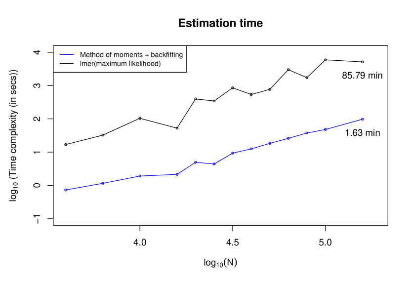
Figure 2: Diagonal case: Comparison of estimation time by the method of moments and backfitting(proposed algorithm) and lmer(existing algorithm)

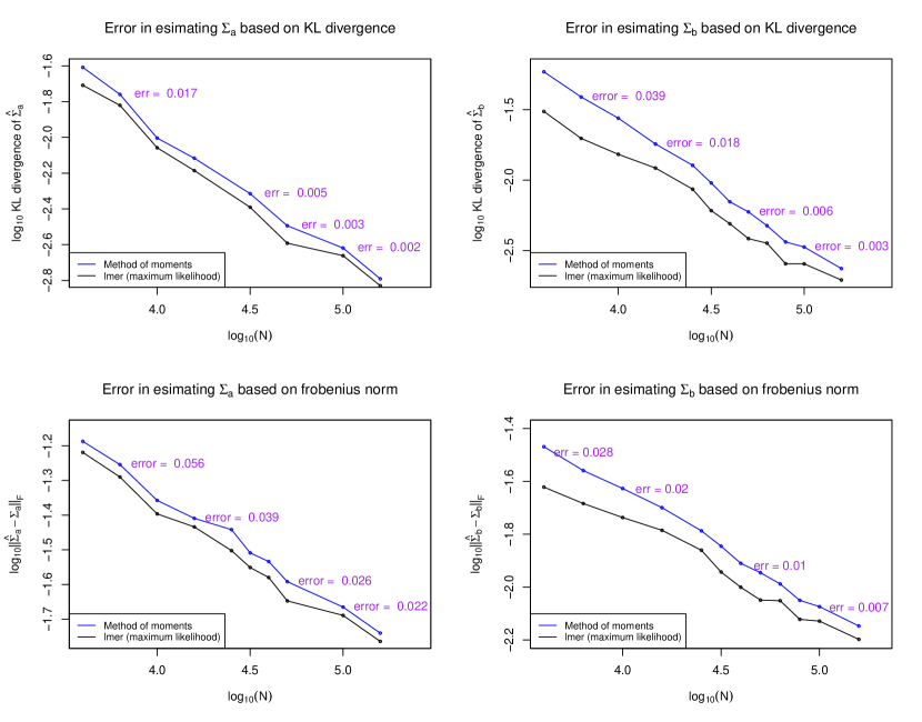
Figure 3: Diagonal case: Comparison of accuracy in estimating ${\Sigma}_{a}$ and ${\Sigma}_{b}$ based on KL divergence and Frobenius norm by the method of moments (proposed algorithm) and lmer(existing algorithm)

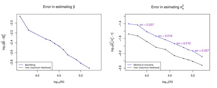
Figure 4: Diagonal case: Comparison of accuracy in estimating $\beta$ and $\sigma^{2}_{e}$ by method of moments (proposed algorithm) and lmer(existing algorithm)

7.1.2 Non diagonal case

For the non-diagonal case, we also choose $p=3,\beta=(0.2,0.3,0.4),\beta_{0}=0.1,\sigma^{2}_{e}=1$. We considered

$$\Sigma_{a}=\Sigma_{b}=\begin{bmatrix}1&0.2&0.2&0.2\\ 0.2&1&0.2&0.2\\ 0.2&0.2&1&0.2\\ 0.2&0.2&0.2&1\\ \end{bmatrix}$$

We choose $R=C=N^{0.6}$ for our simulations similar to the diagonal case. We have proposed the following algorithms

• Backfitting: We estimate covariance parameters using method of moments and then perform backfitting to estimate the fixed parameter.

• Clubbed Backfitting: We estimate covariance parameters using method of Moments and then perform backfitting with clubbing to estimate the fixed parameter.

• Variational EM: We use the method of Moments to get an initial estimate of covariance parameters and then we improve the estimates in each iteration using the variational M-step along with estimating fixed parameters.

• Clubbed Variational EM: Similar to Variational EM, we start with the method of Moment estimates for covariance parameters and improvise them using variational EM. We apply “clubbing” trick while estimating $\beta$ to fasten the convergence.

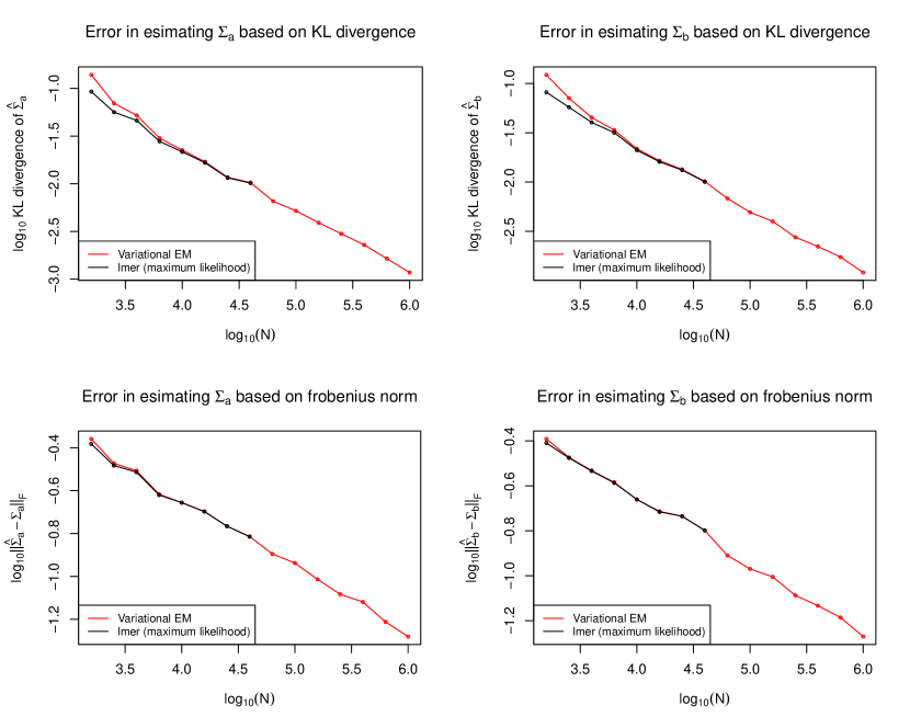
Figure 5: Non-diagonal case: Comparison of accuracy in estimating ${\Sigma}_{a}$ and ${\Sigma}_{b}$ based on KL divergence and Frobenius norm by Variational EM (proposed algorithm) and lmer(existing algorithm). The plot for lmer is discontinued after $N=10^{4.6}$ due to large computational time for “lmer”.

Figure 5 depicts empirical consistency of $\widehat{\Sigma}_{a}$ and $\widehat{\Sigma}_{b}$ as errors explained in 5 go to zero as $n\rightarrow\infty$. Figure 6 shows that the accuracy of different estimates of $\beta$, i.e., $\hat{\beta}_{\mathrm{GLS}}$ obtained though different approaches and $\hat{\beta}_{\mathrm{MLE}}$ coincide and thus $\hat{\beta}_{\mathrm{GLS}}$ is consistent. The estimates of $\sigma^{2}_{e}$ obtained through the method of moments approach and variational EM depict empirical consistency in the figure 6 although the estimate obtained through variational EM has a faster rate of convergence. The figure 7 shows that our variational EM and backfitting approach take a great lead compared to the “lmer” approach. The average time complexity of “lmer” approach is at least $\mathcal{O}(N^{1.5})$ in our setup, while all the approach discussed by us have time complexity $\mathcal{O}(N)$. The number of iterations required to converge grows with $N$ for “lmer” and the approaches without clubbing, while the number of iterations decreases with N for clubbing-based approaches. Here is the summary of results:

	Without Clubbing	With Clubbing
Backftitting	•  Slow convergence	•  Fast Convegence
with MoM	•  Poor estimates for $\Sigma_{a},\Sigma_{b}$	•  Poor estimates for $\Sigma_{a},\Sigma_{b}$
Variational EM	•  Slow convergence	•  Fast Convegence
	•  Good estimates for $\Sigma_{a},\Sigma_{b}$	•  Good estimates for $\Sigma_{a},\Sigma_{b}$

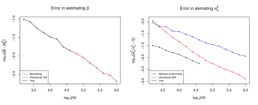
Figure 6: Non diagonal case: Comparison of accuracy in estimating $\beta$ and $\sigma^{2}_{e}$ by Variational EM (proposed algorithm) and lmer(existing algorithm). The plot for lmer is discontinued after $N=10^{4.6}$ due to large computational time for “lmer”. The errors in estimating $\beta$ are close to each other for the illustrated algorithms, which leads the lines in the plot to coincide.

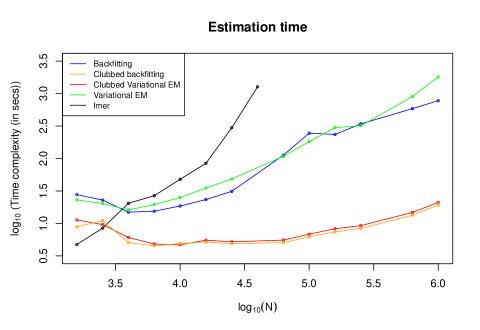
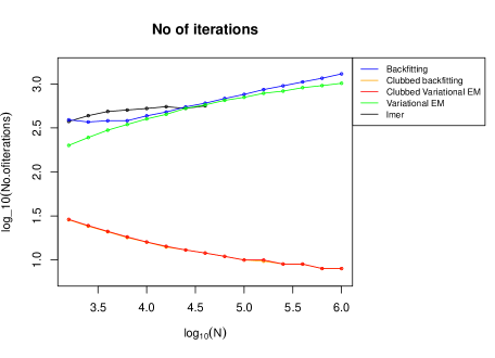
Figure 7: Non-diagonal case: Comparison of estimation time and number of iterations by Backfitting, Clubbed Backftting, Variational EM, and Clubbed Variational EM (four proposed algorithms) and lmer(existing algorithm).

Thus, Clubbed Variational EM provides precise estimates of all the covariance parameters with a small estimation time.

7.2 Real data

Ghosh et al., 2022a applied the backfitting algorithm to obtain $\hat{\beta}_{\mathrm{GLS}}$ for the Stitch FIx data for the random intercepts model $(\ref{eq:intercept_model})$. Here, we demonstrate how our algorithm can be used to apply two crossed-random effects models to the Stitch Fix data. The first model we implement considers a random intercept and a random slope for a variable named “match”, which is a continuous variable taking values in the range 0 to 1 representing the prediction of the probability that the client will keep the item purchased. The second model we implement considers random intercept and random slopes for the variable “match” and multiple indicator variables named “client edgy”, “client boho”, “item edgy”, “item boho”, etc. These refer to fashion styles that describe some items and some client’s preferences. In both of the models, we assume multivariate normal distributions for the random effects for clients as well as items. It should be noted that the purpose of this section is not to choose the most appropriate random effects model. Instead, we wish to illustrate the application of our algorithm in a random slope setup, and we chose a simple default model for that purpose. Along with fitting the models, we also measured the prediction accuracy of these models and compared them with ordinary least squares and the random intercept model.

7.2.1 Random slope for the variable “match”

Here, we implement our devised algorithm to fit the random effects model with a random slope considered for the “match” variable. Thus, the model considered here is,

$$y_{ij}=\tilde{x}^{\mathsf{T}}_{ij}(a_{i}+b_{j})+x_{ij}^{\mathsf{T}}\beta+e_{ij}\hskip 14.22636pt\forall i\in\{1,\cdots,R\}\hskip 8.5359ptj\in\{1,,\cdots,C\},\,$$

where, $\beta$ denotes the fixed effect for the entire covariate vector, $x_{ij}$ listed in table 2. We assume that ${a}_{i}\sim N_{2}(0,{\Sigma}_{a})$ and ${b}_{j}\sim N_{2}(0,{\Sigma}_{b})$ represent random effects for $\tilde{x}_{ij}=(1,\mathrm{match}_{ij})$. The estimate for fixed effect is tabulated in table 2 as $\hat{\beta}_{\mathrm{GLS},1}$. The estimate obtained for $\sigma^{2}_{e}$ is 4.682 and that for $\Sigma_{a}$ and $\Sigma_{b}$ is

$$\widehat{\Sigma_{a}}=\begin{pmatrix}1.817&-1.130\\ -1.130&1.447\\ \end{pmatrix}\hbox{ and }\widehat{\Sigma_{b}}=\begin{pmatrix}0.810&-1.574\\ -1.574&4.163\end{pmatrix}$$

Ghosh et al., 2022a defined naivete and inefficiency of $\mathrm{OLS}$ with respect to the random intercept model to establish the utility of fitting a random effects model. Here we carry the work forward by displaying the naivety and inefficiency of $\mathrm{OLS}$ with respect to the random effects model discussed above. The values of naivete range from 2.63 to 912.36. These values are larger than naivety values reported in  Ghosh et al., 2022a as the largest value reported by them was 345.28. The largest and second-largest ratios are for material indicators corresponding to ‘Modal’ and ‘Tencel’ using the random effects model too. We also identified the linear combination of $\hat{\beta}_{\mathrm{OLS}}$ for which OLS is most naive. We maximize the ratio $x^{\mathsf{T}}\widehat{\mathrm{Cov}}_{\mathrm{GLS},1}(\hat{\beta}_{\mathrm{OLS}})x/x^{\mathsf{T}}\widehat{\mathrm{Cov}}_{\mathrm{OLS}}(\hat{\beta}_{\mathrm{OLS}})x$ over $x\neq 0$. The resulting maximal ratio is the largest eigenvalue of $\widehat{\mathrm{Cov}}_{\mathrm{OLS}}(\hat{\beta}_{\mathrm{OLS}})^{-1}\widehat{\mathrm{Cov}}_{\mathrm{GLS},1}(\hat{\beta}_{\mathrm{OLS}})$ and it is about 984 while the ratio provided for random intercept model in  Ghosh et al., 2022a was 361. We also quantified inefficiency similar to Ghosh et al., 2022a . The figure 8 plots the naivety and inefficiency values. They range from just over 1.06 to 32.03 and can be interpreted as factors by which using OLS reduces the effective sample size. the “match” variable is found to be an outlier in terms of efficiency in our setup too. An important thing to note here is that though OLS is much more naive with respect to the random slopes model compared to the random intercept one, the difference in efficiency is not that huge.

7.2.2 Random slope for variables “match”, “I(client edgy)”, “I(item edgy)”, “I(client edgy)I(item edgy)”, “I(client boho)”, “I(item boho)”, “I(client boho)I(item boho)”

Thus, the model considered here is

$$y_{ij}=\beta_{0}+\tilde{x}^{\mathsf{T}}_{ij}(a_{i}+b_{j})+x_{ij}^{\mathsf{T}}\beta+e_{ij}\hskip 14.22636pt\forall i\in\{1,\cdots,R\}\hskip 8.5359ptj\in\{1,,\cdots,C\}.\,$$ (51)

where, $\beta$ denotes the fixed effect for the entire covariate vector, $x_{ij}$ similar as above. We assume that ${a}_{i}\sim N_{8}(0,{\Sigma}_{a})$ and ${b}_{j}\sim N_{8}(0,{\Sigma}_{b})$ represent random effects for

$$\tilde{x}_{ij} =(1,\mathrm{match}_{ij},\text{I(client edgy})_{i},\text{I(item edgy})_{j},\text{I(client edgy})_{i}\text{I(item edgy})_{j},$$

$$\hskip 56.9055pt\text{I(client boho)}_{i},\text{I(item boho)}_{j},\text{I(client boho)}_{i}\text{I(item boho)}_{j})$$

The estimate obtained for $\sigma^{2}_{e}$ is 5.017 and that for $\Sigma_{a}$ and $\Sigma_{b}$ is

$$\widehat{\Sigma_{a}}=\begin{pmatrix}1.044&-0.223&-0.296&0.015&-0.053&-0.324&0.036&-0.023\\ -0.223&0.912&-0.091&0.011&0&-0.145&0.012&-0.001\\ -0.296&-0.091&0.747&-0.029&-0.022&0.003&-0.009&0.006\\ 0.015&0.011&-0.029&0.426&-0.232&-0.01&-0.003&-0.001\\ -0.053&0&-0.022&-0.232&0.59&0.005&-0.008&0.001\\ -0.324&-0.145&0.003&-0.01&0.005&0.753&-0.02&0.005\\ 0.036&0.012&-0.009&-0.003&-0.008&-0.02&0.563&-0.278\\ -0.023&-0.001&0.006&-0.001&0.001&0.005&-0.278&0.647\end{pmatrix}$$

$$\widehat{\Sigma_{b}}=\begin{pmatrix}0.838&-1.555&0.004&-0.273&0.010&-0.016&-0.216&-0.014\\ -1.555&3.872&-0.030&0.330&0.000&-0.014&0.188&0.057\\ 0.004&-0.030&0.017&0.004&-0.016&0.000&-0.002&-0.002\\ -0.273&0.330&0.004&0.345&-0.032&0.011&0.064&0.007\\ 0.010&0.000&-0.016&-0.032&0.055&-0.003&-0.002&0.003\\ -0.016&-0.014&0.000&0.011&-0.003&0.017&0.014&-0.015\\ -0.216&0.188&-0.002&0.064&-0.002&0.014&0.333&-0.055\\ -0.014&0.057&-0.002&0.007&0.003&-0.015&-0.055&0.059\end{pmatrix}$$

Similar to the first model, we also display the naivete and inefficiency of $\mathrm{OLS}$ with respect to the random effects model 51 discussed above. The values of naivete range from 3.80 to 740.93. The largest and second-largest ratios are for material indicators corresponding to ‘Modal’ and ‘Tencel’ using this random effects model too. We also identified the linear combination of $\hat{\beta}_{\mathrm{OLS}}$ for which OLS is most naive. We maximize the ratio $x^{\mathsf{T}}\widehat{\mathrm{Cov}}_{\mathrm{GLS},1}(\hat{\beta}_{\mathrm{OLS}})x/x^{\mathsf{T}}\widehat{\mathrm{Cov}}_{\mathrm{OLS}}(\hat{\beta}_{\mathrm{OLS}})x$ over $x\neq 0$ similar as above. The resulting maximal ratio is the largest eigenvalue of $\widehat{\mathrm{Cov}}_{\mathrm{OLS}}(\hat{\beta}_{\mathrm{OLS}})^{-1}\widehat{\mathrm{Cov}}_{\mathrm{GLS},1}(\hat{\beta}_{\mathrm{OLS}})$ and it is about 805.59. The figure 8 plots the naivety and inefficiency values. They range from just over 1.02 to 27.34 and can be interpreted as factors by which using OLS reduces the effective sample size. the “match” variable is found to be an outlier in terms of efficiency using this model too. Comparing the naivety and inefficiency values with the previous model, the model with just a random slope for “match” appears to be more effective as it providuces much larger naivety values.

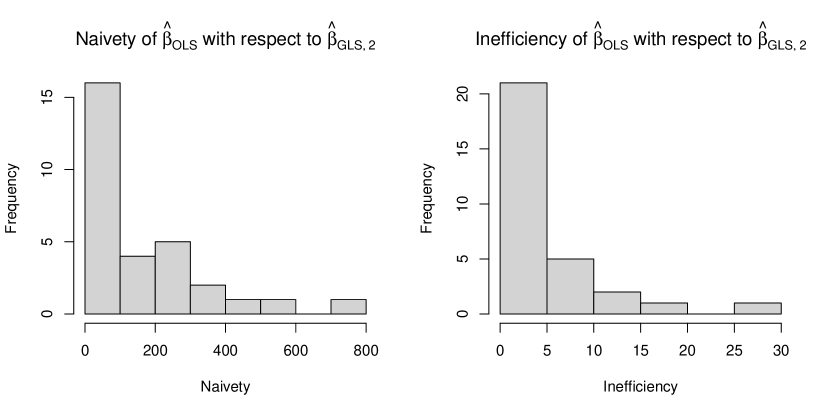
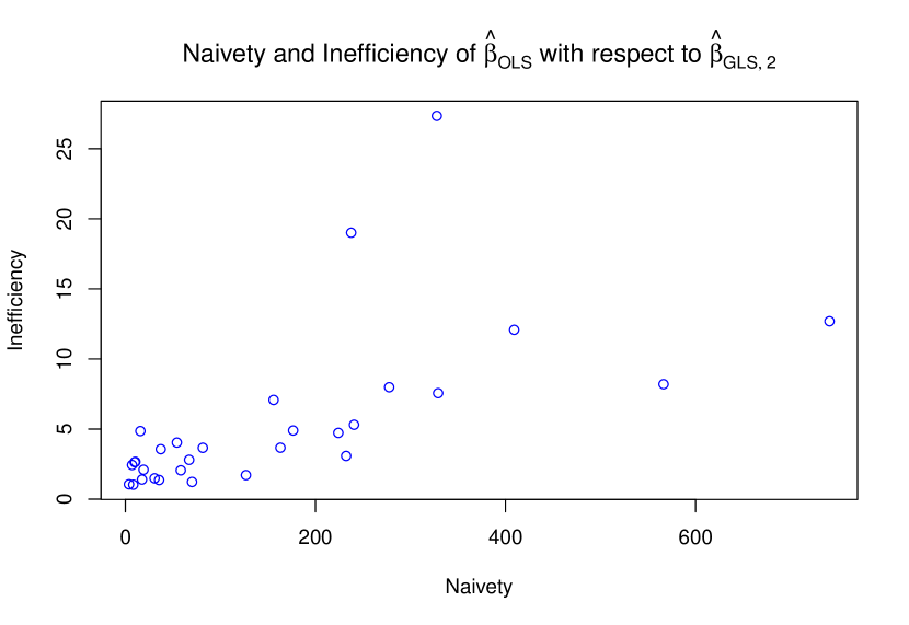
Figure 8: Naivety and efficiency of $\hat{\beta}_{\mathrm{OLS}}$ with respect to $\hat{\beta}_{\mathrm{GLS},1}$

7.3 Prediction error

We considered a random train-test split of Stitch Fix data. We divide the test data into three categories:

• Repeat client and repeat item: The category includes test points with clients whose information was seen in the training data and items whose information was also available in the training data. The prediction of the rating was given by

  $$\hat{Y}_{ij}=x_{ij}^{\mathsf{T}}(\hat{\beta}+\hat{a}_{i}+\hat{b}_{j})$$

  where $\hat{\beta},\hat{a}_{i},$ and $\hat{b}_{j}$ are the estimates of $\beta$ and BLUP estimates of $a_{i}$ and $b_{j}$ repectively.

• New client and repeat item: The category includes test points with clients whose information was not seen in the training data and items whose information was available in the training data. The prediction of the rating was given by

  $$\hat{Y}_{ij}=x_{ij}^{\mathsf{T}}(\hat{\beta}+\hat{b}_{j}),$$

  as the prior expectation for $a_{i}$ is zero.

• Repeat client and new item: The category includes test points with clients whose information was seen in the training data and items whose information was not available in the training data. The prediction of the rating was given by

  $$\hat{Y}_{ij}=x_{ij}^{\mathsf{T}}(\hat{\beta}+\hat{a}_{i}),$$

  as the prior expectation for $b_{j}$ is zero.

We observed only two test data points in the third category, so we are only reporting prediction errors in the first two categories. In the table 1, $\mathrm{GLS}_{0}$ represent the crossed random effects model with random intercepts, $\mathrm{GLS}_{1}$ represent the crossed random effects model with random intercepts and random slope for the variable “match”, and $\mathrm{GLS}_{2}$ represent the crossed random effects model with random intercept and random slope for the variable “match” and random slope for multiple indicator variables discussed above.

	$\mathrm{OLS}$	$\mathrm{GLS}_{0}$	$\mathrm{GLS}_{2}$	$\mathrm{GLS}_{2}$
Repeat client and repeat item	5.710125	4.876266	4.867539	5.525144
New client and repeat item	5.682390	5.604378	5.543491	5.749653

Table 1: Prediction error for different models among different categories

For the first category, we observe 99,115 data points and for the second category, we observe 883 data points. $\mathrm{GLS}_{0}$ provides a significant improvement over $\mathrm{OLS}$ in the first category but the improvement is not much significant for the second category as the information for the clients is not available in the training data. $\mathrm{GLS}_{1}$ provides a small improvement over $\mathrm{GLS}_{0}$ in both of the categories. However, $\mathrm{GLS}_{2}$ provides worse performance compared to $\mathrm{GLS}_{0}$ which reflects a possible overfitting. Thus, if we were to compare models $\mathrm{GLS}_{0}$, $\mathrm{GLS}_{1}$, and $\mathrm{GLS}_{2}$, $\mathrm{GLS}_{1}$ comes out to be the best one. The results are consistent with the naivety and inefficiency values we discussed before.

8 Conclusion

In the paper, we discussed estimation under crossed random effects model with random slopes. We suggested two different algorithms, based on the method of moments combined with backfitting and variational EM. The former is most appropriate when covariance matrices for random effects are diagonal and the latter is useful when the covariance matrices are unstructured. The algorithm based on the method of moments was shown to have theoretical as well as empirical consistency to estimate fixed effects and covariance parameters when covariance matrices for random effects were diagonal. The algorithm based on variational EM was able to accomplish a more difficult task which is to estimate the parameters when the covariance matrices are unstructured and showed great empirical results. Both of the algorithms could complete the task to estimate fixed and covariance parameters in $\mathcal{O}(N)$ and are superior to “lmer” which takes at least $\mathcal{O}(N^{3/2})$. The algorithms find huge applications in settings with large sample sizes and where the time taken to obtain the fit is crucial. We depicted the performance of our algorithms using simulations as well as real data.

Appendix A Some proofs

A.1 Proof of Theorem 1

See 1 where

$$\hat{\beta}_{\mathrm{GLS}}=\operatorname*{arg\,min}_{\beta}(Y-X\beta)\mathcal{V}^{-1}(Y-X\beta)=(X^{\mathsf{T}}\mathcal{V}^{-1}X)^{-1}X^{\mathsf{T}}\mathcal{V}^{-1}Y$$ (12)

Proof.

We rewrite the model as

$$Y=X\beta+ZU+\epsilon\,\,\text{ where, }U\sim N(0,\Sigma_{u}),\text{ and }\epsilon\sim N(0,\sigma^{2}_{e}I)$$

Then,

$$P_{r}(Y=y,U=u)=P_{r}(Y=y)P_{r}(U=u|Y=y)=P_{r}(Y=y|U=u)P_{r}(U=u)$$

$P_{r}(Y=y)$ corresponds to the likelihood in $(\ref{eq:likelihood})$ and $\hat{\beta}_{\mathrm{GLS}}$ in $(\ref{eq:beta})$, and $P_{r}(Y=y|U=u)P_{r}(U=u)$ corresponds to the exponent of $(\ref{eq:loss}$). Now,

$$P_{r}(U=u|Y=y)=\frac{1}{\sqrt{|Var(U|y)|}}\exp\left(-\frac{(u-\mathbb{E}[U|y])^{\mathsf{T}}\left[Var(U|y)\right]^{-1}(u-\mathbb{E}[U|y])}{2}\right)$$

which is maximised for $u=\mathbb{E}[U|Y=y]$, and

$$\max_{u}P_{r}(U=u|Y=y)=\frac{1}{(2\pi)^{(p+1)/2}\sqrt{|Var(U|y)|}}=\mbox{a constant }$$

$$\max_{u}P_{r}(y,U=u)=\max_{u}P_{r}(Y=y)P_{r}(U=u|Y=y)=\mbox{ constant }p(y)$$

Therefore,

$$\operatorname*{arg\,max}_{\beta}\max_{u}P_{r}(Y=y,U=u)=\operatorname*{arg\,max}_{\beta}P_{r}(Y=y)\frac{1}{\sqrt{|Var(U|y)|}}$$

It is understood that $Var(U|y)$ is constant in terms of $\beta$, which implies,

$$\operatorname*{arg\,max}_{\beta}\max_{u}P_{r}(Y=y,U=u)=\operatorname*{arg\,max}_{\beta}P_{r}(Y=y)$$

which is equivalent to saying

$$\hat{\beta}=\hat{\beta}_{\mathrm{GLS}}$$

∎

A.2 Consistency of $\hat{\beta}_{\mathrm{OLS}}$

See 3

Proof.

To begin with, we assume the observations are arranged by the level of the first factor. $Y=X\beta+\epsilon$ where $\epsilon\sim N(0,\mathcal{V})$ for

$$\mathcal{V} =\underbrace{diag(X_{1}^{(a)}\Sigma_{a}X_{1}^{(a)\mathsf{T}},\cdots,X_{R}^{(a)}\Sigma_{a}X_{R}^{(a)\mathsf{T}})}_{B_{R}}$$

$$\hskip 56.9055pt+P_{C}\underbrace{diag(X_{1}^{(b)}\Sigma_{b}X_{1}^{(b)\mathsf{T}},\cdots,X_{C}^{(b)}\Sigma_{b}X_{C}^{(b)\mathsf{T}})}_{B_{C}}P_{C}^{\mathsf{T}}+\sigma^{2}_{e}\bf{I}_{N}$$

with $P_{C}$ being an appropriate permutation matrix. Note that $\hat{\beta}_{\mathrm{OLS}}=\beta+(X^{\mathsf{T}}X)^{-1}X^{\mathsf{T}}\epsilon.$ $\mathbb{E}((X^{\mathsf{T}}X)^{-1}X^{\mathsf{T}}\epsilon)=\bf{0}.$ Let $w$ be any $p\times 1$ vector with finite norm.

$$\mathrm{Var}(w^{\mathsf{T}}(X^{\mathsf{T}}X)^{-1}X^{\mathsf{T}}\epsilon) =w^{\mathsf{T}}(X^{\mathsf{T}}X)^{-1}X^{\mathsf{T}}\mathcal{V}X(X^{\mathsf{T}}X)^{-1}w$$

$$\leq\lambda_{\max}(B_{R})w^{\mathsf{T}}(X^{\mathsf{T}}X)^{-1}w$$

$$\hskip 5.69046pt+\lambda_{\max}(P_{C}B_{C}P_{C}^{\mathsf{T}})w^{\mathsf{T}}(X^{\mathsf{T}}X)^{-1}w+\sigma^{2}_{e}w^{\mathsf{T}}(X^{\mathsf{T}}X)^{-1}w$$

$$\leq\lambda_{\max}(B_{R})\frac{\|w\|^{2}}{cN}+\lambda_{\max}(P_{C}B_{C}P_{C}^{\mathsf{T}})\frac{\|w\|^{2}}{cN}+\sigma^{2}_{e}\frac{\|w\|^{2}}{cN}$$

$$\leq\lambda_{\max}(B_{R})\frac{\|w\|^{2}}{cN}+\lambda_{\max}(B_{C})\frac{\|w\|^{2}}{cN}+\sigma^{2}_{e}\frac{\|w\|^{2}}{cN}\to 0$$

So $\hat{\beta}_{\mathrm{OLS}}$ is consistent estimator for $\beta$. ∎

A.3 Method of Moments

See 4

Proof.

Each of the equations (23), (24), and (25) can be represented as

$$\mathbb{E}\bigg{[}r^{\mathsf{T}}(I-Q)r\bigg{]}=\hat{r}^{\mathsf{T}}(I-Q)\hat{r}\text{ for some }Q\in\mathbb{R}^{N\times N}.$$ (52)

For example, $Q$ for $(\ref{eq:mm1})$ is given by

$$Q=\begin{bmatrix}{\frac{{x^{(s)}_{1.}}x^{(s)^{\mathsf{T}}}_{1.}}{\|{x^{(s)}_{1.}}\|^{2}}}&0&\cdots&0\\ 0&{\frac{{x^{(s)}_{2.}}x^{(s)^{\mathsf{T}}}_{2.}}{\|{x^{(s)}_{2.}}\|^{2}}}&\cdots&0\\ 0&0&\ddots&0\\ 0&0&\cdots&{\frac{{x^{(s)}_{R.}}x^{(s)^{\mathsf{T}}}_{R.}}{\|{x^{(s)}_{R.}}\|^{2}}}\\ \end{bmatrix}$$ (53)

It is sufficient to show that $(\mathbb{E}[r^{\mathsf{T}}(I-Q)r|X]-\hat{r}^{\mathsf{T}}(I-Q)\hat{r})/N$ converges to zero $\forall Q\in\{P_{1},P_{2},\cdots,P_{p},P^{\prime}_{1},\cdots,P^{\prime}_{p},J_{n}\}\text{ and }\forall\,\,\Sigma_{a},\Sigma_{b},\sigma^{2}_{e}$ where $J_{n}=1_{n}1_{n}^{\mathsf{T}}/n$.

$$\frac{\hat{r}^{\mathsf{T}}(I-Q)\hat{r}}{N} =\frac{(\hat{r}-r+r)^{\mathsf{T}}(I-Q)(\hat{r}-r+r)}{N}$$

$$=\frac{r^{\mathsf{T}}(I-Q)r+(\hat{r}-r)^{\mathsf{T}}(I-Q)(\hat{r}-r)+2r^{\mathsf{T}}(I-Q)(\hat{r}-r)}{N}$$

$$=\frac{r^{\mathsf{T}}(I-Q)r}{N}+\frac{(\hat{\beta}_{\mathrm{OLS}}-\beta)^{\mathsf{T}}X^{\mathsf{T}}(I-Q)X(\hat{\beta}_{\mathrm{OLS}}-\beta)}{N}$$

$$\hskip 142.26378pt-\frac{2r^{\mathsf{T}}(I-Q)X(\hat{\beta}_{\mathrm{OLS}}-\beta)}{N}$$

As $x_{ij}$ have finite fourth moment $\forall i\in\{1,\cdots,R\}\,j\in\{1,\cdots,C\}$, $X^{\mathsf{T}}X/N=O_{p}(1)$, and as $\hat{\beta}_{\mathrm{OLS}}$ is consistent, second and third terms converge to zero in probability. Now,

$$\frac{(\hat{r}^{\mathsf{T}}(I-Q)\hat{r}-\mathbb{E}[r^{\mathsf{T}}(I-Q)r|X])}{N} =\frac{r^{\mathsf{T}}(I-Q)r}{N}-\frac{\mathbb{E}[r^{\mathsf{T}}(I-Q)r|X])}{N}+o_{p}(1)$$

Now,

$$\frac{r^{\mathsf{T}}(I-Q)r-\mathbb{E}[r^{\mathsf{T}}(I-Q)r]}{N}\to 0$$ (54)

and

$$\frac{\mathbb{E}[r^{\mathsf{T}}(I-Q)r|X]-\mathbb{E}[r^{\mathsf{T}}(I-Q)r]}{N}\to 0$$ (55)

by the strong law of large numbers assuming finite fourth moment of $x_{ij}$ $\forall i\in\{1,\cdots,R\}$ and $j\in\{1,\cdots,C\}$. Let, $\theta=(diag(\Sigma_{a}),diag(\Sigma_{b}),\sigma^{2}_{e})$, then method of moment estimate, $\theta_{n}$ is solution of equations in the form $A_{n}\theta=B_{n}$, i.e. , $\theta_{n}=A_{n}^{-1}B_{n}$. The above proof guarantees that $A_{n}\to A$ and $B_{n}\to A\theta,\,\,\forall\theta$. Therefore, $\theta_{n}\to\theta$.
∎

A.4 Proof of (26)

We know from (3) that

$$r_{ij}=x_{ij}^{\mathsf{T}}(a_{i}+b_{j})+\epsilon_{ij}$$

It could also be represented as

$$r=\sum_{s^{\prime}=0}^{p}X_{A}^{(s^{\prime})}A_{s^{\prime}}+\sum_{s^{\prime}=0}^{p}X_{B}^{(s^{\prime})}B_{s^{\prime}}+\epsilon$$

Here, $A_{s^{\prime}}\in\mathbb{R}^{R}$ and $B_{s^{\prime}}\in\mathbb{R}^{C}$ represent stacked random coefficient of s’-th coordinate for clients and items respectively, and $X_{A}^{(s^{\prime})}$ and $X_{B}^{(s^{\prime})}$ represent respective design matrices. Then, we have

$$\mathbb{E}\bigg{[}\sum_{i=1}^{R}\sum_{j=1}^{C}z_{ij}r^{2}_{ij}-\sum_{i=1}^{R}\frac{\left(\sum_{j=1}^{C}z_{ij}r_{ij}x^{(s)}_{ij}\right)^{2}}{\sum_{j=1}^{C}z_{ij}x^{2}_{ij(s)}}\bigg{|}X\bigg{]}=\mathbb{E}[r^{\mathsf{T}}(I-Q)r]$$

$$=\mathbb{E}\left(\sum_{s^{\prime}=0}^{p}X_{A}^{(s^{\prime})}A_{s^{\prime}}+\sum_{s^{\prime}=0}^{p}X_{B}^{(s^{\prime})}B_{s^{\prime}}+\epsilon\right)^{\mathsf{T}}\left(I-Q\right)\left(\sum_{s^{\prime}=0}^{p}X_{A}^{(s^{\prime})}A_{s^{\prime}}+\sum_{s^{\prime}=0}^{p}X_{B}^{(s^{\prime})}B_{s^{\prime}}+\epsilon\right)$$

$$=\sum_{s^{\prime}=0}^{p}E\bigg{[}(X_{A}^{(s^{\prime})}A_{s^{\prime}})^{\mathsf{T}}(I-Q)(X_{A}^{(s^{\prime})}A_{s^{\prime}})\bigg{]}+\sum_{s^{\prime}=0}^{p}E\bigg{[}(X_{B}^{(s^{\prime})}B_{s}^{\prime})^{\mathsf{T}}(I-Q)(X_{B}^{(s^{\prime})}B_{s^{\prime}})\bigg{]}$$

$$\hskip 312.9803pt+\sigma^{2}_{e}(n-R)$$

$$=\sum_{s^{\prime}=0}^{p}\operatorname{tr}\bigg{[}X_{A}^{\left(s^{\prime}\right)^{\mathsf{T}}}\left(I-Q\right)X_{A}^{\left(s^{\prime}\right)}\bigg{]}\Sigma_{a,s^{\prime}s^{\prime}}+\sum_{s^{\prime}=0}^{p}\operatorname{tr}\bigg{[}X_{B}^{\left(s^{\prime}\right)^{\mathsf{T}}}\left(I-Q\right)X_{B}^{\left(s^{\prime}\right)}\bigg{]}\Sigma_{b,s^{\prime}s^{\prime}}$$

$$\hskip 312.9803pt+\sigma^{2}_{e}(n-R)$$

$$=\sum_{s^{\prime}=0}^{p}\sum_{i=1}^{R}\left[\sum_{j=1}^{C}z_{ij}x^{(s^{\prime})^{2}}_{ij}-\frac{\left(\sum_{j=1}^{C}z_{ij}x^{(s)}_{ij}x^{(s^{\prime})}_{ij}\right)^{2}}{\sum_{j=1}^{C}z_{ij}x^{(s)^{2}}_{ij}}\right]\Sigma_{a,s^{\prime}s^{\prime}}$$

$$\hskip 85.35826pt+\sum_{s^{\prime}=0}^{p}\sum_{i=1}^{R}\left[\sum_{j=1}^{C}z_{ij}x^{(s^{\prime})^{2}}_{ij}-\frac{\sum_{j=1}^{C}z_{ij}x^{(s)^{2}}_{ij}x^{(s^{\prime})^{2}}_{ij}}{\sum_{j=1}^{C}z_{ij}x^{(s)^{2}}_{ij}}\right]\Sigma_{b,s^{\prime}s^{\prime}}+\sigma^{2}_{e}(n-R)$$

The first part of the last equality follows directly from the definition of $Q$, the last part could be shown using the following argument:
Let,

$$X_{B}^{(s^{\prime})}=\begin{bmatrix}W_{1}\\ W_{2}\\ \vdots\\ W_{R}\end{bmatrix}$$

$$\operatorname{tr}\bigg{[}\left(X_{B}^{(s^{\prime})}\right)^{\mathsf{T}}(I-Q)\left(X_{B}^{(s^{\prime})}\right)\bigg{]} =\sum_{i=1}^{R}\operatorname{tr}\bigg{[}W^{\mathsf{T}}_{i}\left(I-\frac{x^{(s)}_{i.}{x^{(s)}_{i.}}^{\mathsf{T}}}{\|x^{(s)}_{i.}\|^{2}}\right)W_{i}\bigg{]}$$

$$=\sum_{i=1}^{R}\operatorname{tr}(W^{\mathsf{T}}_{i}W_{i})-\frac{\operatorname{tr}\left(x^{(s)^{\mathsf{T}}}_{i.}W_{i}W_{i}^{\mathsf{T}}x^{(s)}_{i.}\right)}{\|x^{(s)}_{i.}\|^{2}}$$

Now,

$$W_{i}W^{\mathsf{T}}_{i}=\begin{bmatrix}{x^{(s^{\prime})}_{i1}}^{2}&0&\cdots&0\\ 0&{x^{(s^{\prime})}_{i2}}^{2}&\cdots&0\\ 0&0&\ddots&0\\ 0&0&0&{x^{(s^{\prime})}_{in_{i}}}^{2}\\ \end{bmatrix}$$

Thus,

$$\operatorname{tr}\bigg{[}\left(X_{B}^{(s^{\prime})}\right)^{\mathsf{T}}(I-Q)\left(X_{B}^{(s^{\prime})}\right)\bigg{]}=\sum_{s^{\prime}=0}^{p}\sum_{i=1}^{R}\left[\sum_{j=1}^{C}z_{ij}x^{(s^{\prime})^{2}}_{ij}-\frac{\sum_{j=1}^{C}z_{ij}x^{(s)^{2}}_{ij}x^{(s^{\prime})^{2}}_{ij}}{\sum_{j=1}^{C}z_{ij}x^{(s)^{2}}_{ij}}\right]$$

The additional equation we added was given by

$$\hat{r}^{\mathsf{T}}\bigg{(}I-\frac{1}{n}11^{\mathsf{T}}\bigg{)}\hat{r}=E\bigg{[}r^{\mathsf{T}}\bigg{(}I-\frac{1}{n}11^{\mathsf{T}}\bigg{)}r\bigg{]}$$

L.H.S. of the above equation will be given by

$$\sum_{i=1}^{R}\sum_{j=1}^{C}z_{ij}\hat{r}^{2}_{ij}-\frac{1}{n}\left(\sum_{i=1}^{R}\sum_{j=1}^{C}z_{ij}\hat{r}_{ij}\right)^{2}$$

For R.H.S., similar to above, we will be needing the following expressions:

$$\operatorname{tr}\bigg{[}(X_{A}^{(s)})^{\mathsf{T}}\bigg{(}I-\frac{1}{n}11^{\mathsf{T}}\bigg{)}(X_{A}^{(s^{\prime})})\bigg{]}=\sum_{i=1}^{R}\bigg{(}\sum_{j=1}^{C}z_{ij}x^{(s)}_{ij}x^{(s^{\prime})}_{ij}-\frac{\sum_{j=1}^{C}z_{ij}x^{(s)}_{ij}\sum_{j=1}^{C}z_{ij}x^{(s^{\prime})}_{ij}}{n}\bigg{)}$$

and

$$\operatorname{tr}\bigg{[}(X_{B}^{(s)})^{\mathsf{T}}\bigg{(}I-\frac{1}{n}11^{\mathsf{T}}\bigg{)}(X_{B}^{(s^{\prime})})\bigg{]}=\sum_{j=1}^{C}\bigg{(}\sum_{i=1}^{R}z_{ij}x^{(s)}_{ij}x^{(s^{\prime})}_{ij}-\frac{\sum_{i=1}^{R}z_{ij}x^{(s)}_{ij}\sum_{i=1}^{R}z_{ij}x^{(s^{\prime})}_{ij}}{n}\bigg{)}$$

A.5 Proof of Lemma 1

$$q_{a}^{k} (a_{1},\cdots,a_{R})\propto\mathbb{P}(y,\{a_{i}\}_{i=1}^{R}|b_{j}=E_{Q^{(k-1)}}[b_{j}])$$

$$\propto\exp\left\{-\frac{1}{2}\sum_{i=1}^{R}\sum_{j=1}^{C}\frac{z_{ij}(y_{ij}-x_{ij}^{\mathsf{T}}(a_{i}+\mu_{b,j}^{(k-1)}+\beta))^{2}}{\left(\sigma^{(k-1)}_{e}\right)^{2}}-\frac{1}{2}\sum_{i=1}^{R}a_{i}^{\mathsf{T}}(\Sigma_{a}^{(k-1)})^{-1}a_{i}\right\}$$

$$\propto\exp\Bigg{\{}-\frac{1}{2}\sum_{i=1}^{R}a_{i}^{\mathsf{T}}\Bigg{(}(\Sigma^{(k-1)}_{a})^{-1}+\frac{\sum_{j=1}^{C}z_{ij}x_{ij}x_{ij}^{\mathsf{T}}}{\left(\sigma^{(k-1)}_{e}\right)^{2}}\Bigg{)}a_{i}$$

$$\hskip 56.9055pt+a_{i}^{\mathsf{T}}\frac{\sum_{j=1}^{C}z_{ij}\big{(}y_{ij}-x_{ij}^{\mathsf{T}}\big{(}\beta^{(k-1)}+\mu^{(k-1)}_{b,j}\big{)}\big{)}x_{ij}}{\left(\sigma^{(k-1)}_{e}\right)^{2}}\Bigg{\}}$$

Thus,

$$\mu^{(k)}_{a,i}=\Sigma^{(k)}_{a,i}\left(\frac{\sum_{j=1}^{C}z_{ij}\big{(}y_{ij}-x_{ij}^{\mathsf{T}}\big{(}\beta^{(k-1)}+\mu^{(k-1)}_{b,j}\big{)}\big{)}x_{ij}}{\left(\sigma^{(k-1)}_{e}\right)^{2}}\right)$$

and

$$\Sigma^{(k)}_{a,i}=\left((\Sigma^{(k-1)}_{a})^{-1}+\frac{\sum_{j=1}^{C}z_{ij}x_{ij}x_{ij}^{\mathsf{T}}}{\left(\sigma^{(k-1)}_{e}\right)^{2}}\right)^{-1}$$

$$q_{b}^{k} (b_{1},\cdots,b_{C})\propto\mathbb{P}(y,\{b_{j}\}_{j=1}^{C}|a_{i}=E_{Q^{(k)}}[a_{i}])$$

$$\propto\exp\left\{-\frac{1}{2}\sum_{j=1}^{C}\sum_{i=1}^{R}\frac{z_{ij}(y_{ij}-x_{ij}^{\mathsf{T}}(b_{j}+\mu_{a,i}^{(k)}+\beta))^{2}}{\left(\sigma^{(k-1)}_{e}\right)^{2}}-\frac{1}{2}\sum_{j=1}^{C}b_{j}^{\mathsf{T}}(\Sigma_{b}^{(k-1)})^{-1}b_{j}\right\}$$

$$\propto\exp\Bigg{\{}-\frac{1}{2}\sum_{j=1}^{C}b_{j}^{\mathsf{T}}\Bigg{(}(\Sigma^{(k-1)}_{b})^{-1}+\frac{\sum_{i=1}^{R}z_{ij}x_{ij}x_{ij}^{\mathsf{T}}}{\left(\sigma^{(k-1)}_{e}\right)^{2}}\Bigg{)}b_{j}$$

$$\hskip 56.9055pt+b)j^{\mathsf{T}}\frac{\sum_{j=1}^{C}z_{ij}\big{(}y_{ij}-x_{ij}^{\mathsf{T}}\big{(}\beta^{(k-1)}+\mu^{(k)}_{a,i}\big{)}\big{)}x_{ij}}{\left(\sigma^{(k-1)}_{e}\right)^{2}}\Bigg{\}}$$

Thus,

$$\mu^{(k)}_{b,j}=\Sigma^{(k)}_{b,j}\left(\frac{\sum_{i=1}^{R}z_{ij}\big{(}y_{ij}-x_{ij}^{\mathsf{T}}\big{(}\beta^{(k-1)}+\mu^{(k-1)}_{a,i}\big{)}\big{)}x_{ij}}{\left(\sigma^{(k-1)}_{e}\right)^{2}}\right)$$

and

$$\Sigma^{(k)}_{b,j}=\left((\Sigma^{(k-1)}_{b})^{-1}+\frac{\sum_{i=1}^{R}z_{ij}x_{ij}x_{ij}^{\mathsf{T}}}{\left(\sigma^{(k-1)}_{e}\right)^{2}}\right)^{-1}$$

A.6 Fixed effects for Stitch FIx data

	$\hat{\beta}_{\mathrm{OLS}}$	$\hat{\beta}_{\mathrm{GLS}.0}$	$\hat{\beta}_{\mathrm{GLS}.1}$	$\hat{\beta}_{\mathrm{GLS}.2}$
Intercept	4.635*	5.103*	5.148*	5.134*
Match	5.048*	3.442*	3.306*	3.336*
$\mathbb{I}\{\text{ client edgy }\}$	0.00102	0.00304	-0.00038	0.00038*
$\mathbb{I}\{\text{ item edgy }\}$	-0.3358*	-0.3515*	-0.3660*	-0.3916*
$\mathbb{I}\{\text{ client edgy }\}$
$*\mathbb{I}\{\text{ item edgy }\}$	$0.3925^{*}$	$0.3793^{*}$	$0.3775^{*}$	0.4132*
$\mathbb{I}\{\text{ client boho }\}$	0.1386*	0.1296*	0.1313*	0.1399*
$\mathbb{I}\{\text{ item boho }\}$	-0.5499*	-0.6266*	-0.6269*	-0.6670*
$\mathbb{I}\{\text{ client boho }\}$
$*\mathbb{I}\{\text{ item boho }\}$	$0.3822^{*}$	$0.3763^{*}$	$0.3734^{*}$	0.4137*
Acrylic	-0.06482*	-0.00536	0.0110	0.03440*
Angora	-0.0126	0.07486	0.09617	0.10050*
Bamboo	-0.04593	0.03251	0.07282	0.07346*
Cashmere	-0.1955*	0.00893	0.02474	0.05574*
Cotton	0.1752*	0.1033*	0.1191*	0.1261*
Cupro	0.5979	0.2089	0.0530	0.0749
Faux Fur	0.2759*	0.2749	0.2832*	0.2914*
Fur	-0.2021*	-0.07924	-0.07745	-0.14690*
Leather	0.2677*	0.1674*	0.1569	0.1536*
Linen	-0.3844*	-0.08658	-0.0844	0.1160*
Modal	0.0026	0.1388*	0.1316	0.1436*
Nylon	0.0335*	0.08174	0.0899	0.0826*
Patent Leather	-0.2359	-0.3764	-0.5184	0.3763
Pleather	0.4163*	0.3292*	0.3504*	0.3516*
PU	0.416*	0.4579*	0.4517*	04618*
PVC	0.6574*	0.9688*	0.8535	0.7729*
Rayon	-0.01109*	0.05155*	0.0637*	0.05638*
Silk	-0.1422*	-0.1828*	-0.2160*	-0.2022*
Spandex	-0.3916*	0.414*	0.4074*	0.4099*
Tencel	0.4966*	0.1234*	0.1176	0.1422*
Viscose	0.04066*	-0.02259	-0.03238	-0.03795*
Wool	-0.0602*	-0.05883	-0.06684	-0.04681*

Table 2: Stitch Fix results

References

- Bates et al., (2015) Bates, D., Mächler, M., Bolker, B., and Walker, S. (2015). Fitting linear mixed-effects models using lme4. Journal of Statistical Software, 67(1):1–48.
- Beal and Ghahramani, (2003) Beal, M. and Ghahramani, Z. (2003). The variational bayesian em algorithm for incomplete data: with application to scoring graphical model structures. Bayesian Statistics, 7(2):000–000.
- Buja et al., (1989) Buja, A., Hastie, T., and Tibshirani, R. (1989). Linear smoothers and additive models (with discussion). The Annals of Statistics, 17(2):453–510.
- Gao and Owen, (2017) Gao, K. and Owen, A. B. (2017). Efficient moment calculations for variance components in large unbalanced crossed random effects designs. Electronic Journal of Statistics, 11(1):1235–1296.
- Gao and Owen, (2020) Gao, K. and Owen, A. B. (2020). Estimation and inference for very large linear mixed effects models. Statistica Sinica, 30:1741–1771.
- Ghosh, (2022) Ghosh, S. (2022). Scalable inference for crossed random effects models. PhD thesis, Stanford University.
- (7) Ghosh, S., Hastie, T., and Owen, A. B. (2022a). Backfitting for large scale crossed random effects regressions. Annals of Statistics, 50(1):560–583.
- (8) Ghosh, S., Hastie, T., and Owen, A. B. (2022b). Scalable logistic regression with crossed random effects. Electronic Journal of Statistics, 16(2):4604–4635.
- Ghosh and Zhong, (2021) Ghosh, S. and Zhong, C. (2021). Convergence rate of a collapsed gibbs sampler for crossed random effects models. Technical report, arxiv:2109.02849.
- Goplerud, (2021) Goplerud, M. (2021). Fast and accurate estimation of non-nested binomial hierarchical models using variational inference. Bayesian Analysis, -1.
- Papaspiliopoulos et al., (2020) Papaspiliopoulos, O., Roberts, G. O., and Zanella, G. (2020). Scalable inference for crossed random effects models. Biometrika, 107(1):25–40.
- Robinson, (1991) Robinson, G. (1991). That BLUP is a good thing: the estimation of random effects. Statistical Science, 6(1):15–51.