An axiomatized PDE model of deep neural networks

Abstract

Inspired by the relation between deep neural network (DNN) and partial differential equations (PDEs), we study the general form of the PDE models of deep neural networks. To achieve this goal, we formulate DNN as an evolution operator from a simple base model. Based on several reasonable assumptions, we prove that the evolution operator is actually determined by convection-diffusion equation. This convection-diffusion equation model gives mathematical explanation for several effective networks. Moreover, we show that the convection-diffusion model improves the robustness and reduces the Rademacher complexity. Based on the convection-diffusion equation, we design a new training method for ResNets. Experiments validate the performance of the proposed method.

35K57, 93B35

1 Introduction

Deep neural networks (DNN) have achieved success in tasks such as image classification [33], speech recognition [7], video analysis [3], and action recognition [39]. Among these networks, residual networks (ResNets) are important architectures, making it practical to train ultra-deep DNN, and has ability to avoid gradient vanishing [12, 13]. Also, the idea of ResNets has motivated the development of many other DNNs including WideResNet [43], ResNeXt  [41], and DenseNet  [15].

In recent years, understanding the ResNets from the dynamical perspective has become a promising approach [8, 11]. More specifically, assume ${\bm{x}}_{0}\in\mathbb{R}^{d}$ as the input of ResNet [12] and define $\mathcal{F}$ to be a mapping, then the $l$-th residual block can be realized by

(1) $${\bm{x}}_{l+1}={\bm{x}}_{l}+\mathcal{F}({\bm{x}}_{l},{\bm{w}}_{l})$$

where ${\bm{x}}_{l}$ and ${\bm{x}}_{l+1}$ are the input and output tensors of the residual mapping, and ${\bm{w}}_{l}$ are parameters of $l$-th layer that are learned by minimizing the training error. Define ${\bm{x}}_{L}$ as the output of a ResNet with $L$ layers, then the classification score is determined by ${\bm{y}}=\mathrm{softmax}({\bm{w}}_{\text{fc}}{\bm{x}}_{L})$, where ${\bm{w}}_{\text{fc}}$ are also learnable parameters of the final linear layer.

For any $T>0$, introducing a temporal partition $\Delta t=T/L$, the ResNet represented by Eq. 1 is the explicit Euler discretization with time step $\Delta t$ of the following differential equation:

(2) $$\frac{{\rm d}{\bm{x}}(t)}{{\rm d}t}=v({\bm{x}}(t),t),\quad{\bm{x}}(0)={\bm{x}}_{0}\quad t\in[0,T],$$

where $v({\bm{x}}(t),t)$ is a velocity field such that $\Delta tv({\bm{x}}(t),t)=F({\bm{x}}(t),{\bm{w}}(t))$. The above ordinary differential equation (ODE) interpretation of ResNet provides new perspective and has inspired many networks. As shown in [25], by applying stable and different numerical methods for Eq. 2, it leads to PolyNet [45] and FractalNet [21]. Besides, the other direction is to consider the the continuous form of Eq. 2, representing the velocity $v({\bm{x}},t)$ by a deep neural network. One typical method is the Neural ODE [4] in which $v$ is updated by the adjoint state method. Similar extensions along this direction include neural stochastic differential equation (SDE) [17] and neural jump SDE [18]. The theoretical property of these continuous models has been analyzed in  [37, 2, 44].

The connection between ODE and partial differential equation (PDE) through the well-known characteristics method has motivated the analysis of ResNet from PDE perspective, including theoretical analysis [34], novel training algorithms [36] and improvement of adversarial robustness [38] for DNNs. To be specific, from the PDE theory, the ODE Eq. 2 is the characteristic curve of the transport equation:

(3) $$\frac{\partial u}{\partial t}({\bm{x}},t)=-v({\bm{x}},t)\nabla u({\bm{x}},t),~{}({\bm{x}},t)\in\mathbb{R}^{d}\times[0,T].$$

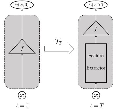
Figure 1: $\mathcal{T}_{T}$ is the map between two colored boxes. The left represents the base linear classifier. Right represents feature extractor + linear classifier, which together form a typical neural network.

The method of characteristics tells us that, along the curve $({\bm{x}},t)$ defined by Eq. 2, the function value $u({\bm{x}},t)$ remains unchanged. Assume at $t=T$, $u({\bm{x}},T)=f({\bm{x}})\coloneqq\mathrm{softmax}({\bm{w}}_{\text{fc}}{\bm{x}})$ is the linear classifier, then

$$u({\bm{x}}(0),0)=u({\bm{x}}(T),T)=f({\bm{x}}(T))=f\circ k({\bm{x}}(0))$$

where $k$ represents the mapping from ${\bm{x}}(0)$ to ${\bm{x}}(T)$, which is the continuous form of feature extraction in ResNet. Thus at $t=0$, $u(\cdot,0)$ is the composition of a feature extractor and a classifier, which is analogous to ResNet. Nonetheless, since the transport equation Eq. 3 is reversible in time, and initial value problem is more common than terminal value problem in PDE, we assume $u({\bm{x}},0)=f({\bm{x}})$ in our paper. Consequently, the direction of solving ODE Eq. 2 needs to be reversed, but its connection to ResNet remains consistent. In one word, the transport equation Eq. 3 can describe the evolution from a linear classifier to ResNet.

Suppose we fix the initial condition $u(\cdot,0)$ as the linear classifier $f$. DNN can be seen as a map between two functions: $u(\cdot,0)$ and $u(\cdot,T)$. In ResNets, this map is formulated as a convection equation. A natural question is: Is convection equation is the only PDE to formulate this map? If not, can we derive a general form of PDE to formulate the map? In this paper, we try to answer above questions from mathematical point of view. First we construct a continuous flow $\mathcal{T}_{t}$ which maps a simple linear classifier to a more complicate function, as illustrated in Fig. 1,

(4) $$\mathcal{T}_{t}:f\mapsto u(\cdot,t),\quad t\in[0,T],$$

The idea in this paper is also classical in mathematics. First, we extract some basic properties $\mathcal{T}_{t}$ should satisfies. Then based on these basis properties, a general form of $\mathcal{T}_{t}$ can be derived rigorously. More specifically, inspired by the scale space theory, we prove that under several reasonable assumptions on $\mathcal{T}_{t}$, $u({\bm{x}},t)=\mathcal{T}_{t}f({\bm{x}})$ is the solution of a second order convection-diffusion equation. This theoretical result provides a unified framework which covers transport equation and some existing works including Gaussian noise injection [38, 24], dropout techniques [36, 35] and randomized smoothing [5, 23, 31]. It also illuminates new thinking for designing networks. In summary, we list the main contributions as follows.

• We establish several basic assumptions on operator $\mathcal{T}_{t}$, and prove the sufficiency of these assumptions for generalizing ResNet and beyond. To the best of our knowledge, this is the first theoretical attempt for establishing a sufficient condition for designing the variants of ResNet from the PDE perspective, which may provide some insights when considering the search space in neural architecture search (NAS).

• Inspired by our theoretical analysis, we propose an isotropic model by adding isotropic diffusion to Eq. 3. Compared to the linear classifier $f$, we prove that the proposed model has lower Rademacher complexity and larger region with certified robustness. Moreover, we design a training method by applying the operator splitting scheme for solving the proposed convection-diffusion equation.

Notations

We denote scalars, vectors, and matrices by lowercase and uppercase letters, where vectors and matrices are bolded. We denote the $\ell_{2}$ and $\ell_{\infty}$ norms of the vector ${\bm{x}}=(x_{1},\cdots,x_{d})\in\mathbb{R}^{d}$ by $\|{\bm{x}}\|_{2}={(\sum_{i=1}^{d}|x_{i}|^{2})^{1/2}}$ and $\|{\bm{x}}\|_{\infty}=\max_{i=1}^{d}|x_{i}|$, respectively. We denote the gradient and Laplace operators by $\nabla=(\frac{\partial}{\partial x_{1}},\cdots,\frac{\partial}{\partial x_{d}})$ and $\Delta=\sum^{d}_{i=1}\frac{\partial^{2}}{\partial x^{2}_{i}}$, respectively. For a function $f:\mathbb{R}^{d}\rightarrow\mathbb{R}$, $D^{\alpha}f$ denotes its $\alpha$-order derivative, $\|f({\bm{x}})\|_{L^{\infty}}=\sup_{{\bm{x}}\in\mathbb{R}^{d}}|f({\bm{x}})|$ its $L^{\infty}$ norm. $\mathcal{N}(\mathbf{0},\sigma^{2}{\mathbf{I}})$ denotes Gaussian noise with mean $\mathbf{0}$ and variance $\sigma^{2}$. $C^{\infty}_{b}$ is the space of bounded functions which have bounded derivatives at any order.

2 General PDE model

In this section, we show under several reasonable assumptions, the sequence of operator images $u({\bm{x}},t)=\mathcal{T}_{t}f({\bm{x}})$ is the solution of the convection-diffusion equation. Then we show that our convection-diffusion equation model can naturally cover various existing effective models.

2.1 The characterization of $\mathcal{T}_{t}$

Throughout this section, we assume $\mathcal{T}_{t}$ is well defined on $C^{\infty}_{b}$, and $\mathcal{T}_{t}f$ is a bounded continuous function. The assumption is reasonable, since typical classifiers $f$ like a linear classifier is indeed bounded (between 0 and 1) and has bounded derivatives. The operator image $\mathcal{T}_{t}f$, which we hope to be a neural network, is obviously bounded and continuous. To get the expression of the evolution operator $\mathcal{T}_{t}$, we assume it has some fundamental properties, which fall into two categories: deep neural network type and partial differential equation type.

2.1.1 DNN-type assumptions

Suppose we are given two classifiers $f$ and $g$ such that $f({\bm{x}})\geq g({\bm{x}})$ for all data point ${\bm{x}}\in\mathbb{R}^{d}$. Then $f\circ k({\bm{x}})\geq$ $g\circ k({\bm{x}})$ if we replace the data points with extracted features. Recall that for ResNet, $f\circ k=\mathcal{T}_{T}(f)$, which implies $\mathcal{T}_{T}\left(f\right)\geq\mathcal{T}_{T}\left(g\right)$. Since the order-preserving property holds both at initial time step $t=0$ and final time step $t=T$, it is reasonable to make the following assumption

[Comparison Principle] For all $t\geq 0$ and $f,g\in C^{\infty}_{b}$, if $f\leq g$, then $\mathcal{T}_{t}(f)\leq\mathcal{T}_{t}(g)$.

The prediction of a deep neural network is computed using forward propagation, i.e. the network uses output of former layer as input of current layer. Thus, for a DNN model, it’s natural that the output of a DNN can be deduced from the output of intermediate $l$-th layer without any information depending upon the original data point ${\bm{x}}$ and output of $m$-th layer ($m<l$). Regarding the evolution of operator $\mathcal{T}_{t}$ as stacking layers in the neural network, we should require that $\mathcal{T}_{t+s}$ can be computed from $\mathcal{T}_{t}$ for any $s\geq 0$, and $T_{0}$ is of course the identity, which implies

[Markov Property] $\mathcal{T}_{t+s}=\mathcal{\mathcal{missing}}T_{t}\circ T_{t+s,t}$, for all $s,t\geq 0$ and $t+s\leq T$. $\mathcal{T}_{t+s,t}$ denotes the flow from time $t$ to time $t+s$.

Linearity is also an intrinsic property of deep neural networks. Notice that we are not referring to a single DNN’s output v.s. input linearity, which is obviously wrong because of the activation function. Rather, we are stating that two different DNN with the same feature extractor can be merged in to a new DNN with a new classifier composed with the shared extractor, i.e.

$$(\beta_{1}f+\beta_{2}g)\circ k=\beta_{1}f\circ k+\beta_{2}g\circ k$$

This is linearity at $t=T$, and for $t=0$ it is trivial. Thus we assume,

[Linearity] For any $f,g\in C^{\infty}_{b}$, and real constants $\beta_{1},\beta_{2}$, we have

$$\mathcal{T}_{t}(\beta_{1}f+\beta_{2}g)=\beta_{1}\mathcal{T}_{t}(f)+\beta_{2}\mathcal{T}_{t}(g)$$

if $C$ is a constant function, then $\mathcal{T}_{t}(C)=C$.

2.1.2 PDE-type assumptions

First of all, we need an assumption to ensure the existence of a differential equation. If two classifiers $f$ and $g$ have the same derivatives of any order at some point, then we should assume same evolution at this point when $t$ is small. If we unrigorously define $\partial T_{t}(f)/\partial t=\left(\mathcal{T}_{t}(f)-f\right)/t$ when $t\rightarrow 0^{+}$ (or infinitesimal generator in our proof), then $\partial T_{t}(f)/\partial t$ should equal to $\partial T_{t}(g)/\partial t$. Thus, we give the following assumption concerning the local character of the operator $\mathcal{T}_{t}$ for $t$ small.

[Locality] For all fixed ${\bm{x}}$, if $f,g\in C_{b}^{\infty}$ satisfy $D^{\alpha}f({\bm{x}})=D^{\alpha}g({\bm{x}})$ for all $|\alpha|\geq 0$, then

$$\lim_{t\rightarrow 0^{+}}\frac{(\mathcal{T}_{t}(f)-\mathcal{T}_{t}(g))({\bm{x}})}{t}=0$$

Regularity is an essential component in PDE theory. Thus, when considering PDE-type assumptions on $\mathcal{T}_{t}$, it is necessary to study its regularity. We separate the regularity requirements into spatial and temporal. First, spatial regularity means that if we add a perturbation ${\bm{h}}$ to data point ${\bm{x}}$, the output $\mathcal{T}_{t}(f)({\bm{x}}+{\bm{h}})$ will not be much different from adding the same perturbation to the output $\mathcal{T}_{t}(f)({\bm{x}})$. One can relate it to the well-known translation invariance in image processing, but our assumption is weaker, as we allow small difference rather than require strict equivalence,

[Spatial Regularity] There exist a positive constant $C$ dependening on $f$ such that

$$\|\mathcal{T}_{t}(\tau_{{\bm{h}}}f)-\tau_{{\bm{h}}}(\mathcal{T}_{t}f)\|_{L^{\infty}}\leq Cht$$

for all $f\in C^{\infty}_{b},{\bm{h}}\in\mathbb{R}^{d},t\geq 0$, where $(\tau_{{\bm{h}}}f)({\bm{x}})=f({\bm{x}}+{\bm{h}})$ and $\|{\bm{h}}\|_{2}=h$.

Remark 2.1.

Spatial regularity is also beneficial for adversarial robustness. DNN have been shown to be vulnerable to some well-designed input samples (adversarial examples) [10, 20]. These adversarial examples are produced by adding carefully hand-crafted perturbations to the inputs of the targeted model. Although these perturbations are imperceptible to human eyes, they can fool DNN to make wrong prediction. In some sense, the existence of these adversarial examples is due to spatial unstability of DNN. So in our method, we hope the new model $\mathcal{T}_{t}(f)$ to be spatially stable.

Secondly, temporal stability requires that in any small time interval, the evolution process will not be rapid. We want a smooth operator $\mathcal{T}_{t}$ in time. Our assumption goes

[Temporal Regularity] For all $t,s,t+s\in[0,T]$ and all $f\in C^{\infty}_{b}$, there exist a constant $C\geq 0$ depending on $f$ such that

$$\|\mathcal{T}_{t+s,s}(f)-f\|_{L^{\infty}} \leq Ct$$

$$\|\mathcal{T}_{t+s,s}(f)-\mathcal{T}_{t}(f)\|_{L^{\infty}} \leq Cst$$

Finally, combine all the assumptions on $\mathcal{T}_{t}$, we can derive the following theorem, emphasizing that the output value of neural network $T_{t}(f)$ with time evolution satisfies a convection-diffusion equation,

Theorem 2.2.

Under the above assumptions, there exists Lipschitz continuous function $v:\mathbb{R}^{d}\times[0,T]\to\mathbb{R}^{d}$ and Lipschitz continuous positive function $\sigma:\mathbb{R}^{d}\times[0,T]\to\mathbb{R}^{d\times d}$ such that for any bounded and uniformly continuous base classifier $f({\bm{x}})$, $u({\bm{x}},t)=\mathcal{T}_{t}(f)({\bm{x}})$ is the unique solution of the following convection-diffusion equation:

(5) $$\begin{cases}\frac{\partial u({\bm{x}},t)}{\partial t}=v({\bm{x}},t)\cdot\nabla u({\bm{x}},t)+\sum_{i,j}\sigma_{i,j}\frac{\partial^{2}u}{\partial x_{i}\partial x_{j}}({\bm{x}},t),\\ u({\bm{x}},0)=f({\bm{x}}),\end{cases}$$

where ${\bm{x}}\in\mathbb{R}^{d},t\in[0,T]$. Here $\sigma_{i,j}$ is the $i,j$-th element of matrix function $\sigma({\bm{x}},t)$.

Remark 2.3.

The right hands of the differential equation in Eq. 5 consist of two terms, the first order term $v({\bm{x}},t)\cdot\nabla u({\bm{x}},t)$ called convection term and the second order term $\sum_{i,j}\sigma_{i,j}\frac{\partial^{2}u}{\partial x_{i}\partial x_{j}}({\bm{x}},t)$ called diffusion term.

Remark 2.4.

When $\sigma({\bm{x}},t)=\sigma^{2}{\mathbf{I}}$, we call these type equations isotropic equations and the corresponding models isotropic models. When $\sigma({\bm{x}},t)$ is a diagonal matrix and $\sigma({\bm{x}},t)\neq\sigma^{2}{\mathbf{I}}$, we call these type equations anisotropic equations that lead to anisotropic models.

We will provide the proof of Theorem 2.2 in Appendix A. In this subsection, we have introduced a convection-diffusion equation framework for ResNets. The framework is quite general, as many existing models with residual connections can be interpreted as special cases in our framework.

2.2 Examples Convection-Diffusion Model

Under the convection-diffusion framework, we can give interpretation to several regularization mechanisms including Gaussian noise injection [38, 24], ResNet with stochastic dropping out the hidden state of residual block [35, 36] and randomized smoothing [5, 23, 31]. Actually, they can be seen as convection-diffusion model with different diffusion term. Corresponding diffusion terms of these models are listed in Table 1.

Table 1: Examples of networks under our proposed framework

Models	Diffusion terms
ResNet	0
Gaussian noise injection	$\sigma^{2}\Delta u$
Dropout of Hidden Units	$\frac{1-p}{2p}\sum_{i}(v^{T}v)_{i,i}\frac{\partial^{2}u}{\partial x_{i}^{2}}$
Randomized smoothing	$\sigma^{2}\Delta u$

Gaussian noise injection: Gaussian noise injection is an effective regularization mechanism for a DNN model. For a vanilla ResNet with $L$ residual mapping, the $n$-th residual mapping with Gaussian noise injected can be written as

$${\bm{x}}_{n+1}={\bm{x}}_{n}+\mathcal{F}({\bm{x}}_{n},{\bm{w}}_{n})+a\bm{\varepsilon}_{n},\,\,\,\bm{\varepsilon}_{n}\sim\mathcal{N}(0,\mathbf{I})$$

where the parameter $a$ is a noise coefficient. By introducing a temporal partition: $t_{n}=nT/L$, for $n=0,1,..,L$ with the time interval $\Delta t=T/L$ and let ${\bm{x}}(t_{n})={\bm{x}}_{n}$ and ${\bm{w}}(t_{n})={\bm{w}}_{n}$. And let $a=\sigma\sqrt{\Delta t}$ and $\mathcal{F}({\bm{x}}_{n},{\bm{w}}_{n})/\Delta t=v({\bm{x}},t)$. This noise injection technique in a discrete neural network can be viewed as the approximation of continuous dynamic

(6) $$d{\bm{x}}(t)=v({\bm{x}}_{n},t)dt+\sigma d\mathbf{B}(t)$$

where $\mathbf{B}(t)$ is multidimensional Brownian motion. The output of $L$-th residual mapping can be written as I$\hat{t}$o process Eq. 6 at terminal time $T$, ${\bm{x}}(T)$. So, an ensemble prediction over all the possible sub-networks with shared parameters can be written as

(7) $$\hat{y}=\mathbb{E}({\rm softmax}({\bm{w}}_{\text{fc}}{\bm{x}}(T))|{\bm{x}}(0)={\bm{x}}_{0}).$$

According to Feynman-Kac formula [26], Equation 7 is known to solve the following convection-diffusion equation

$$\begin{cases}\frac{\partial u({\bm{x}},t)}{\partial t}=v({\bm{x}},t)\cdot\nabla u+\sigma^{2}\Delta u,\quad{\bm{x}}\in\mathbb{R}^{d},t\in[0,T]\\ u({\bm{x}},0)={\rm softmax}({\bm{w}}_{\text{fc}}{\bm{x}}).\end{cases}$$

Dropout of Hidden Units: Consider the case that we disable every hidden units independently from a Bernoulli distribution $\mathcal{B}(1,p)$ with $p\in(0,1)$ in each residual mapping

$${\bm{x}}_{n+1} = {\bm{x}}_{n}+\mathcal{F}({\bm{x}}_{n},{\bm{w}}_{n})\odot\frac{{\bm{z}}_{n}}{p}$$

$$= {\bm{x}}_{n}+\mathcal{F}({\bm{x}}_{n},{\bm{w}}_{n})+\mathcal{F}({\bm{x}}_{n},{\bm{w}}_{n})\odot(\frac{{\bm{z}}_{n}}{p}-\textbf{I})$$

where ${\bm{z}}_{n}\sim\mathcal{B}(1,p)$ namely $\mathbb{P}({\bm{z}}_{n}=0)=1-p$, $\mathbb{P}({\bm{z}}_{n}=1)=p$ and $\odot$ indicates the Hadamard product. If the number of the ensemble is large enough, according to Central Limit Theorem, we have

$$\mathcal{F}({\bm{x}}_{n},{\bm{w}}_{n})\odot(\frac{{\bm{z}}_{n}}{p}-\textbf{I})\approx\mathcal{F}({\bm{x}}_{n},{\bm{w}}_{n})\odot\mathcal{N}(0,\frac{1-p}{p})$$

The similar way with Gaussian noise injection, the ensemble prediction $\hat{y}$ can be viewed as the solution $u({\bm{x}},T)$ of following equation:

$$\begin{cases}\frac{\partial u({\bm{x}},t)}{\partial t}=v({\bm{x}},t)\cdot\nabla u({\bm{x}},t)+\frac{1-p}{2p}\sum_{i}(v^{T}v)_{i,i}\frac{\partial^{2}u}{\partial x_{i}^{2}}({\bm{x}},t),\quad{\bm{x}}\in\mathbb{R}^{d},t\in[0,T]\\ u({\bm{x}},0)={\rm softmax}({\bm{w}}_{\text{fc}}{\bm{x}}),\end{cases}$$

Remark 2.5.

In fact, similar to dropout, shake-shake regularization [9, 14] and ResNet with stochastic depth [16] can also be interpreted by our convection-diffusion equation model.

Randomized Smoothing: Consider to transform a trained classifier into a new smoothed classifier by adding Gaussian noise to the input when inference time. If we denote the trained classifier by $f({\bm{x}})$ and denote the new smoothed classifier by $g({\bm{x}})$. Then $f({\bm{x}})$ and $g({\bm{x}})$ have the following relation:

$$g({\bm{x}})=\frac{1}{N}\sum^{N}_{i=1}f({\bm{x}}+\bm{\varepsilon}_{i})\approx\mathbb{E}_{\bm{\varepsilon}\sim\mathcal{N}(0,\sigma^{2}I)}[f({\bm{x}}+\bm{\varepsilon})]$$

where $\bm{\varepsilon}_{i}\sim\mathcal{N}(0,\sigma^{2}I)$. According to Feynman-Kac formula, $g({\bm{x}})$ can be viewed as the solution of the following PDEs

(8) $$\begin{cases}\frac{\partial u({\bm{x}},t)}{\partial t}=\frac{1}{2}\sigma^{2}\Delta u,t\in[0,1]\\ u({\bm{x}},0)=f({\bm{x}}).\end{cases}$$

Especially, when $f({\bm{x}})$ is ResNet, the smoothed classifier $g({\bm{x}})=u({\bm{x}},T+1)$ can be expressed as

$$\begin{cases}\frac{\partial u({\bm{x}},t)}{\partial t}=v({\bm{x}},t)\cdot\nabla u({\bm{x}},t),{\bm{x}}\in\mathbb{R}^{d},t\in[0,T]\\ \frac{\partial u({\bm{x}},t)}{\partial t}=\frac{1}{2}\sigma^{2}\Delta u,t\in[T,T+1]\\ u({\bm{x}},0)={\rm softmax}({\bm{w}}_{\text{fc}}{\bm{x}}).\end{cases}$$

The differential equation formulation of randomized smoothing is similar to our method presented in the next section. However, randomized smoothing is a postprocessing step which ensures certified robustness. It does not involve the training of velocity field $v$, which is parametrized by a neural network. Moreover, our method adds regularization term in each time step $t$, while randomized smoothing only adds Gaussian noise on initial time step $t=0$.

Obviously, ResNet is no diffusion model, Gaussian noise injection and randomized smoothing are isotropic models and dropout of hidden units is anisotropic models.

The viewpoint that forward propagation of a ResNet is the solving process of a TE enables us to interpret poor robustness and generalizability as the irregularity of the solution. Moreover, we can also interpret the effectiveness of the models above-mentioned in improving generalizability as the action of diffusion term. Next, we focus on the case of isotropic models, because anisotropic models are difficult for theoretical analysis and practical experiment and we take it as our future work.

3 Theoretical Analysis

In this section, under our convection-diffusion model, we focus on isotropic-type equation. Furthermore, for the sake of simplicity and practical computation, we consider the model with split convection and diffusion in time.

(9) $$\begin{cases}\frac{\partial u(\bm{x},t)}{\partial t}=v(\bm{x},t)\cdot\nabla u(\bm{x},t),&\quad{\bm{x}}\in\mathbb{R}^{d},\quad t\in[0,T-1]\\ \frac{\partial u(\bm{x},t)}{\partial t}=\sigma^{2}\Delta u,&\quad{\bm{x}}\in\mathbb{R}^{d},\quad t\in[T-1,T]\\ u(\bm{x},0)=f(\bm{x})\end{cases}$$

In the following subsections, we will theoretically illustrate its benefits for improving the robustness and reducing the Rademacher complexity of neural networks.

3.1 Robustness guarantee

Assume the data point lies in a bounded domain $\mathcal{D}$. Consider a multi-class classification problem from $\mathcal{D}\subset\mathbb{R}^{d}$ to label class $\mathcal{Y}=\{1,\cdots,k\}$. Let $G$ be a prediction function defined by $G({\bm{x}})=\arg\max_{i\in\mathcal{Y}}u^{i}({\bm{x}},T)$, where $u^{i}({\bm{x}},T)$ is the $i$-th element of $u({\bm{x}},T)$. Suppose that DNN classifies ${\bm{x}}$ the most probable class $c_{A}$ is returned with probability $p_{A}=u^{c_{A}}({\bm{x}},T)$, and the “runner-up” class is returned with probability $p_{B}$. Our main result of this subsection is to estimate the area around the data point ${\bm{x}}$ in which the prediction $G({\bm{x}})$ is robust,

Theorem 3.1.

Suppose the velocity $v({\bm{x}},t)$ is a continuous function $\mathbb{R}^{d}\times[0,T]$ which satisfies the Lipschitz condition, i.e. there exists a given constant $L>0$, such that

$$\|v({\bm{x}}_{1},t)-v({\bm{x}}_{2},t)\|\leq L\|{\bm{x}}_{1}-{\bm{x}}_{2}\|,\quad\forall({\bm{x}}_{1},t),({\bm{x}}_{2},t)\in\mathbb{R}^{d}\times[0,T]$$

Let $u({\bm{x}},T)$ be the bounded solution of Equation 9. Suppose $c_{A}\in\mathcal{Y}$ and

$$u^{c_{A}}({\bm{x}},T)=p_{A}\geq p_{B}=\max_{i\neq c_{A}}u^{i}({\bm{x}},T),$$

then $G({\bm{x}}+\bm{\delta})=c_{A}$ for all $\|\bm{\delta}\|_{2}\leq R$, where

$$R=\frac{\sigma}{\sqrt{2d}}(p_{A}-p_{B})$$

Remark 3.2.

We assume $v$ as Lipschitz continuous because $v(\bm{x},t)=\frac{1}{\Delta t}F(\bm{x},\bm{w})$ corresponds to a residual block, so its gradient can be bounded easily using the network parameters $\bm{w}$.

We provide the proof of Theorem 3.1 in Appendix B. According to Theorem 3.1, we can obtain the certified radius $R$ is large when the diffusion coefficient $\sigma^{2}$ and the probability of the top class is high. We will also consider the generalization ability of model Equation 9 in the next subsection.

3.2 Rademacher complexity

For simplicity, we consider binary classification problems. Assume that data points are drawn from the underlying distribution $\mathcal{D}$. The training set $S_{N}=\{{\bm{x}}_{i}\}_{i=1}^{N}$ is composed of $N$ samples drawn i.i.d. from $\mathcal{D}$. Rademacher complexity is one of the classic measures of generalization error. We first recap on the definition of empirical Rademacher complexity.

Definition 3.3 ([22]).

Let $\mathcal{H}:X\rightarrow{\mathbb{R}}$ be the space of real-valued functions on the space $X$. For a given sample set $S_{N}=\{{\bm{x}}_{i}\}_{i=1}^{N}$, the empirical Rademacher complexity of $\mathcal{H}$ is defined as

$$R_{S_{N}}(\mathcal{H}):=\frac{1}{N}\mathbb{E}_{\sigma}[\sup_{h\in\mathcal{H}}\sum_{i=1}^{N}\sigma_{i}h({\bm{x}}_{i})]$$

where $\sigma_{1},\sigma_{2},\cdots,\sigma_{N}$ are i.i.d. Rademacher random variables with $\mathbb{P}(\sigma_{i}=1)=\mathbb{P}(\sigma_{i}=-1)=\frac{1}{2}$.

Rademacher complexity is a tool to bound the generalization error. The smaller the generalization gap is, the less overfitting the model is. We are interested in the empirical Rademacher complexity of the following function class:

$$\mathcal{G_{\sigma}}:=\Big{\{}g({\bm{x}})=\mathcal{T}_{T}(f)|f\in\mathcal{F}\Big{\}}$$

where

$$\mathcal{F}:=\left\{f:{\bm{x}}\mapsto\phi({\bm{w}}_{\text{fc}}{\bm{x}})|\left\|{\bm{w}}_{\text{fc}}\right\|_{1}\leq W\right\}$$

Here $\mathcal{T}_{t}$ is the solution operator of Eq. 9, $\phi$ is sigmoid activation function. The function class $\mathcal{F}$ represents the hypothesis linear classifiers function class, where we assume the $\ell^{1}$ norm of the weight of fully-connected layer is bounded by $W$. The function class $\mathcal{G}_{\sigma}$ includes the evolved residual neural networks from base classifiers. We can also assume the data points are bounded by $R$, which is reasonable, e.g. in CIFAR-10 dataset [19], the pixel values lie in $[0,1]$. Then we have the following theorem.

Theorem 3.4.

Given a data set $S_{N}=\{{\bm{x}}_{i}\}_{i=1}^{N}$. Suppose the data points $\|{\bm{x}}_{i}\|_{\infty}\leq R$ for ${\bm{x}}_{i}\in S_{N}$, then

$$R_{S_{N}}(\mathcal{G_{\sigma}})\leq R_{S_{N}}(\mathcal{F})\leq\inf_{\epsilon}\left(\sqrt{\frac{2d\log(3WR/\epsilon)}{N}}+\epsilon\right)$$

We provide the proof of Theorem 3.4 in Appendix C. According to Theorem 3.4, we can obtain that the empirical Rademacher complexity of $\mathcal{G}_{\sigma}$ can be upper bounded by that of a simple linear classifier. This can help bounding the generalization error of the evolved neural network. In the next section, we will present a training method for ResNet to verify our results.

4 Training Algorithm

To verify the effectiveness of the convection-diffusion model, we design a training method for ResNet. We assume that the data point lies in an unknown domain $\mathcal{D}\subset\mathbb{R}^{d}$ and the label function $l({\bm{x}})$ is defined on $\mathcal{D}$. Let $\mathcal{S}=\{({\bm{x}}_{i},y_{i})\}^{N}_{i=1}\subset\mathcal{D}$ be the training set, where ${\bm{x}}_{i}$ is a data point sampled from $\mathcal{D}$ and $y_{i}=l({\bm{x}}_{i})$ is the corresponding label.

As stated in the introduction, the forward propagation of ResNet corresponds to the transport equation. Denote ResNet as $g_{\theta}$ with trainable parameters $\theta$. Then the process from $0$ to $T-1$ in model Eq. 9 corresponds to the forward propagation of $g_{\theta}$. In other words, the transport equation part in the convection-diffusion model Eq. 9 is already inherently included in $g_{\theta}$. To incorporate the diffusion part, we enforce the network $g_{\theta}$ to satisfy the following constraint

(10) $$\begin{cases}\frac{\partial g_{\theta}({\bm{x}},t)}{\partial t}=\sigma^{2}\Delta g_{\theta}({\bm{x}},t),&{\bm{x}}\in\mathcal{D},t\in[0,1]\\ g_{\theta}({\bm{x}},t)=l({\bm{x}}),&{\bm{x}}\in\mathcal{S},t\in[0,1]\end{cases}$$

where we set $T-1$ as the new initial time. The first equation is the diffusion part in convection-diffusion model Eq. 9. The second equation is the boundary condition for points in the training set. It is natural to require the network to classify training data correctly at any time $t\in[0,1]$. To impose the constraints, we follow the techniques in PINN [30] and design two loss terms for the boundary condition and differential equation respectively.

First, to fit the boundary condition, we use the following loss

$$L_{1}=\int_{\mathcal{S}}\int_{0}^{1}l^{\text{CE}}\left(g_{\theta}({\bm{x}},s),l({\bm{x}})\right)\mathrm{d}s\mathrm{d}{\bm{x}}\approx\frac{1}{MN}\sum^{N}_{i=1}\sum_{k=1}^{M}l^{\text{CE}}(g_{\theta}({\bm{x}}_{i},t_{k}),y_{i})$$

where $l^{\text{CE}}$ denotes cross-entropy loss. $N$ is the number of data points in $\mathcal{S}$, and $M$ is the number of time steps. In practice, we evenly choose $t_{k}=(k-1)/(M-1)$ to discretize time.

Then, to fit the differential equation, we use the following mean square error loss

$$L_{2}=\int_{\mathcal{D}}\int^{1}_{0}\left(\frac{\partial g_{\theta}}{\partial t}({\bm{x}},s)-\sigma^{2}\Delta g_{\theta}({\bm{x}},s)\right)^{2}\mathrm{d}s\mathrm{d}{\bm{x}}$$

In practice, we only have access to the training set $\mathcal{S}$ and do not know the underlying domain $\mathcal{D}$, thus we treat the neighborhood of $\mathcal{S}$ as the domain. The neighborhood is obtained by adding a uniform noise $\epsilon$ to $\mathcal{S}$. Then the integral term is approximated by

$$L_{2} \approx \frac{1}{N}\sum^{N}_{i=1}\int^{1}_{0}\left(\frac{\partial g_{\theta}}{\partial t}({\bm{x}}_{i}+\epsilon,s)-\sigma^{2}\Delta g_{\theta}({\bm{x}}_{i}+\epsilon,s)\right)^{2}\mathrm{d}s$$

$$\approx \frac{1}{MN}\sum^{N}_{i=1}\sum_{k=1}^{M}\left(\frac{\partial g_{\theta}}{\partial t}({\bm{x}}_{i}+\epsilon,t_{k})-\sigma^{2}\Delta g_{\theta}({\bm{x}}_{i}+\epsilon,t_{k})\right)^{2}.$$

Nonetheless, in neural network, the exact computation of Laplace of output w.r.t the input is computationally intractable [27] because of the high dimension inputs, e.g. for CIFAR-10 pictures the dimension is 3072. Thus, we use finite difference method to approximate. Denote difference operator $\Delta_{h,\bm{v}}$ by

$$\Delta_{h,\bm{v}}g_{\theta}({\bm{x}}_{i},s)=\frac{g_{\theta}({\bm{x}}_{i}+h\bm{v},s)+g_{\theta}({\bm{x}}_{i}-h\bm{v},s)-2g_{\theta}({\bm{x}}_{i},s)}{h^{2}}$$

Using Taylor formula and law of large numbers, we have

$$\Delta g_{\theta}({\bm{x}}_{i},s)=\mathbb{E}_{\bm{v}\sim\mathcal{N}(0,I)}\left(\Delta_{h,\bm{v}}g_{\theta}({\bm{x}}_{i},s)\right)+O(h^{2})\approx\frac{1}{K}\sum^{K}_{j=1}\Delta_{h,\bm{v}_{i,j}}g_{\theta}({\bm{x}}_{i},s)$$

where $\{\bm{v}_{i,j}\}$ is i.i.d and standard normal distributed, $K$ is the average number. Unless otherwise specified, we set $K$ equals 1 in order to reduce the computation cost. Similarly, we introduce the time differential operator $\textbf{dt}_{\tau}$,

$$\textbf{dt}_{\tau}g_{\theta}({\bm{x}}_{i},s)=\frac{g_{\theta}({\bm{x}}_{i},s+\tau)-g_{\theta}({\bm{x}}_{i},s-\tau)}{2\tau}$$

to substitute for $\frac{\partial g_{\theta}}{\partial t}$. Include these difference operators into $L_{2}$, now the loss term for differential equation becomes

$$L_{2}=\frac{1}{MN}\sum^{N}_{i=1}\sum_{k=1}^{M}\left(\textbf{dt}_{\tau}g_{\theta}({\bm{x}}_{i}+\epsilon,t_{k})-\sigma^{2}\frac{1}{K}\sum^{K}_{j=1}\Delta_{h,\bm{v}_{i,j}}g_{\theta}({\bm{x}}_{i}+\epsilon,t_{k})\right)^{2}$$

The final loss function for training $g_{\theta}$ is a weighted sum of $L_{1}$ and $L_{2}$, $L=L_{1}+\lambda L_{2}$.

Since the input of ResNet $g_{\theta}$ is $({\bm{x}},t)$, which now contains an additional time variable $t$, we modify the network input dimension from $[C\times H\times W]$ to $[(C+1)\times H\times W]$, where the additional channal represents $t$. Accordingly, we slightly change the structure of ResNet by adding an additional channel in the first convolution layer. Other than that, our ResNet structure is the same as vanilla ResNet. Obviously, when $t=0$, the additional channel has no impact on the network output, and it functions as same as vanilla ResNet.

5 Experiments

In this section, we will numerically verify the performance of our training method for ResNets.

5.1 Preliminaries

Datasets

In our experiments, we consider both synthetic half-moon dataset and real-world CIFAR-10 [19], Fashion-MNIST [40] and SVHN [28] datasets. Half-moon dataset is a randomly generated 2d synthetic dataset in which we randomly generate 500 points and 1000 points with a standard deviation of 0.3 as training set and testing set, respectively. CIFAR-10 contains 60K $3\times 32\times 32$ color images from 10 different classes with 50K and 10K of them used for training and testing, respectively. SVHN is a 10-class house number classification dataset which contains 73257 training images and 26032 testing images, each of size $3\times 32\times 32$. Fashion-MNIST is a 10-class greyscale dataset which contains 60K training images and 10K testing images. The size of each image is $28\times 28$.

Performance evaluations

We evaluate the performance by both natural accuracy on original test samples and robust accuracy on adversarial test samples within a perturbation range $\epsilon$. To craft adversarial samples, we use Project Gradient Descent (PGD) and AutoAttack [6]. PGD first adds random uniform noise from $(-\epsilon,\epsilon)$ to clean samples, and iterates Fast Gradient Sign Method (FGSM) with fixed step size $\alpha$ for $m$ steps,

$${\bm{x}}^{(m)}={\rm Clip}_{{\bm{x}},\epsilon}\{{\bm{x}}^{(m-1)}+\alpha{\rm sign}(\nabla\mathcal{L}({\bm{x}}^{(m-1)},y))\}$$

AutoAttack [6] is a more reliable benchmark for evaluating robustness, which ensembles four strong parameter-free attacks. It is reported that some defense methods which claim to be robust against PGD attack are destroyed by AutoAttack. Thus, we report classification accuracy on adversarial examples crafted by AutoAttack to evaluate the robustness of our method.

For half-moon dataset, we apply PGD²⁰ (step number $m=20$) attack with $\alpha=0.01$ and $\epsilon=0.2$ under $l^{\infty}$ norm. For CIFAR-10 and SVHN, we apply PGD²⁰ attack with $\alpha=2/255$ and $\epsilon=8/255$. For Fashion-MNIST, we apply PGD²⁰ attack with $\alpha=0.01$ and $\epsilon=0.1$. AutoAttack is parameter-free and thus we only set $\epsilon$ as same as that of PGD attack.

5.2 Experiments on synthetic dataset

In this subsection, we numerically verify the efficacy of our training method in improving the robustness of ResNet on the half-moon dataset.

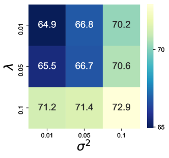
Figure 2: Robust accuracy of ResNet trained by our model with different hyperparameters $\lambda$ and $\sigma^{2}$ on half-moon dataset.

We first vary hyperparameters $\lambda$ and $\sigma^{2}$ and present the classification accuracy on adversarial examples in Figure 2. The robust accuracy increase when $\lambda$ and $\sigma^{2}$ increase, which indicates that the introduced regularizer is helpful for improving the performance of ResNet. Moreover, we plot the decision boundary of naturally trained ResNet and ResNet trained with different $\lambda,\sigma^{2}$ in Figure 3. We can obvserve that the decision boundary of natural training is irregular, while that of our models is smoother. These experimental results are consistent with our theory.

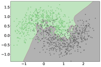
(a) Natural training

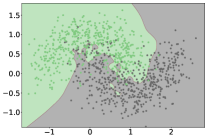
(b) $\lambda=0.01,\sigma^{2}=0.01$

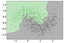
(c) $\lambda=0.1,\sigma^{2}=0.01$

(d) $\lambda=0.1,\sigma^{2}=0.1$

Figure 3: Decision boundary of natural trained ResNet and ResNet trained by our method with different hyperparameters $\lambda$ and $\sigma^{2}$.

5.3 Experiment on benchmarks

Table 2: Natural accuracy and robust accuracy under PGD²⁰ and AutoAttack on different datasets (%).

Dataset	Methods	Natural	PGD20	AutoAttack
CIFAR-10	ResNet18	95.18	0.0	0.0
	Ours	88.54	20.02	17.64
SVHN	ResNet18	96.58	0.40	0.02
	Ours	94.16	19.05	15.48
Fashion-MNIST	ResNet18	93.95	0.0	0.0
	Ours	92.01	35.27	23.48

We further test the performance of our method on CIFAR-10, SVHN and Fashion-MNIST datasets. We choose ResNet18 as the backbone model, where our method will add an additional channel in the input convolutional layer. During training, we apply standard data augmentation techniques including random crops and horizontal flips. The batch size is 128. We run 200 epochs with initial learning rate of 0.1, which decays by a factor of 10 at the 80th, 120th and 160th epochs. We use stochastic gradient descent optimizer with momentum of 0.9 and weight decay of $5\times 10^{-4}$.

Table 3: Natural accuracy and robust accuracy under PGD²⁰ and AutoAttack on CIFAR-10, with varying parameter $\lambda$ and $\sigma^{2}$ (%).

$\lambda$	$\sigma^{2}$	Natural	PGD20	AutoAttack
0.2	0.2	80.33	24.91	23.89
0.1	0.2	82.64	24.04	22.97
0.05	0.2	84.51	23.58	22.53
0.01	0.2	87.45	20.63	18.37
0.005	0.2	88.54	20.02	17.64
0.2	0.1	81.79	20.56	19.74
0.1	0.1	84.73	20.02	18.87
0.05	0.1	85.95	19.07	17.76
0.01	0.1	89.52	18.60	14.12
0.005	0.1	89.95	15.22	11.11

There are several hyperparameters in our algorithm that need to be determined. $h$ and $\tau$ are spatial and temporal discretization parameters. We choose $\tau=10^{-4}$ and $h=0.1$. We choose a fairly large $h$ because neural networks are highly unstable on the spatial dimension and cannot converge when $h$ is too small. To reduce the computation cost, we choose $K=1$ when computing the Laplacian $\Delta$, and only consider starting and final time step $t_{1}=0,t_{2}=1$ when computing the regularization loss. The uniform noise $\epsilon$ which we add to training set $\mathcal{S}$ to fit the underlying domain $\mathcal{D}$ is chosen the same as the attack range of each dataset, i.e. $8/255$ for CIFAR-10 and SVHN, and $0.1$ for Fashion-MNIST. $\lambda$ and $\sigma^{2}$ both affect the trade-off between natural accuracy and robust accuracy. With larger $\lambda$ or $\sigma^{2}$, the natural accuracy decreases, while robust accuracy increases. We report the result of $\lambda=0.005$ and $\sigma^{2}=0.2$ in Table 2, and an ablation study on the two parameters can be found in Table 3. From Table 2, we can see that our method, which introduces a regularization term based on convection-diffusion differential equation, raises the classification accuracy of ResNet against adversarial samples by a large margin. We want to emphasize that our method does not include any adversarial training techniques, which trains the model using adversarial samples crafted by PGD attacks. From Table 3, we observe that with fixed parameter $\sigma^{2}$, the natural accuracy decreases and robust accuracy increases as the increasing of parameters $\lambda$ and vice versa.

6 Conclusion

In this paper, we theoretically prove that under reasonable assumptions, the evolution from a base linear classifier to residual neural networks should be modeled by a convection-diffusion equation. Motivated by PDE theory, we analyze the robustness and Rademacher complexity of the proposed isotropic models. Based on these theoretical results, we develop a training method for ResNet and verify its effectiveness through experiments. We are aware that modeling the convection-diffusion equation through introducing a regularization term is one of the many possible approaches. We are looking forward to explore other paths in the future work.

Appendices

Appendix A Proof of Theorem 2.2

Proof A.1.

Following the techniques in [1], we set

$$\delta_{t,s}(f)=\frac{\mathcal{T}_{t}(f)-\mathcal{T}_{s}(f)}{t-s},\quad\delta_{t}(f)=\delta_{t,0}(f)$$

The proof of Theorem 2.2 mainly consists of two steps. First we will prove that $\delta_{t}(f)$ converges to a limit as $t\rightarrow 0$, which we call an infinitesimal generator. Then, we verify that the generator satisfy a second-order convection-diffusion equation.

First of all, we describe some basic properties of $\delta_{t}(f)$. From [Temporal Regularity], we know $\delta_{t}(f)$ is uniformly bounded,

$$\|\delta_{t}(f)\|_{L^{\infty}}=\left\|\frac{\mathcal{T}_{t}(f)-f}{t}\right\|_{L^{\infty}}\leq C$$

Also, it is obvious that [Linearity] is preserved for $\delta_{t}(f)$,

$$\delta_{t}(\beta_{1}f+\beta_{2}g)=\beta_{1}\delta_{t}(f)+\beta_{2}\delta_{t}(g)$$

Additionally, $\delta_{t}(f)$ is Lipschitz continuous on $\mathbb{R}^{d}$, uniformly for $t\in(0,1]$ and $f\in C^{\infty}_{b}$. Indeed, let ${\bm{h}}\in\mathbb{R}^{d},\|{\bm{h}}\|_{2}=h$,

$$\|\tau_{{\bm{h}}}(\delta_{t}(f))-\delta_{t}(f)\|_{L^{\infty}}\leq\|\tau_{{\bm{h}}}(\delta_{t}(f))-\delta_{t}(\tau_{{\bm{h}}}f)\|_{L^{\infty}}+\|\delta_{t}(\tau_{{\bm{h}}}f)-\delta_{t}(f)\|_{L^{\infty}}$$

The first term can be bounded using [Spatial Regularity],

$$\|\tau_{{\bm{h}}}(\delta_{t}(f))-\delta_{t}(\tau_{{\bm{h}}}f)\|_{L^{\infty}}=\left\|\frac{\tau_{{\bm{h}}}(\mathcal{T}_{t}f)-\mathcal{T}_{t}(\tau_{{\bm{h}}}f)}{t}\right\|_{L^{\infty}}\leq Ch$$

The second term can be bounded using the fact that $f\in C^{\infty}_{b}$. We may write $\tau_{{\bm{h}}}f=f+hg$ for some $g\in C^{\infty}_{b}$ depending on ${\bm{h}}$, then using linearity and uniform boundedness,

$$\|\delta_{t}(\tau_{{\bm{h}}}f)-\delta_{t}(f)\|_{L^{\infty}}=\|\delta_{t}(f+hg)-\delta_{t}(f)\|_{L^{\infty}}=h\|\delta_{t}(g)\|_{L^{\infty}}\leq Ch$$

Lastly, since $f\leq g+\|f-g\|_{L^{\infty}}$, we can use [Comparison Principle] and [Linearity] to get

$$\mathcal{T}_{t}(f)\leq\mathcal{T}_{t}(g+\|f-g\|_{L^{\infty}})=\mathcal{T}_{t}(g)+\|f-g\|_{L^{\infty}}$$

Thus for any $f,g\in C^{\infty}_{b}$ and $t\geq 0$,

(11) $$\|\mathcal{T}_{t}(f)-\mathcal{T}_{t}(g)\|_{L^{\infty}}\leq\|f-g\|_{L^{\infty}}$$

Now we are ready to prove the main theorem.

A.1 Existence of infinitesimal generator

First we want to prove:

(12) $$\|\delta_{t+s,t}(f)-\delta_{s}(f)\|_{L^{\infty}}\leq m(t)$$

where $m(t)$ is some continuous, nonnegative, nondecreasing function such that $m(0)=0$, and $m(t)$ depends only on the bounds of derivatives of $f$.

Since $\delta_{s}(f)$ not necessarily belongs to $C^{\infty}_{b}$, we mollify $\delta_{s}(f)$ by introducing a standard mollifier $K\geq 0$ satisfying $\int_{\mathbb{R}^{d}}K\mathrm{d}{\bm{y}}=1$, $K\in C_{0}^{\infty}(\mathbb{R}^{d})$ and $K_{\varepsilon}=\varepsilon^{-d}K(\cdot/\varepsilon)$. Using the Lipschitz continuity of $\delta_{s}(f)$, we can obtain that for all $\varepsilon>0$, there exist a positive constant $C_{1}$ depending only on the derivatives of $f$, such that

(13) $$\|\delta_{s}(f)\ast K_{\varepsilon}-\delta_{s}(f)\|_{L^{\infty}}\leq C_{1}\varepsilon.$$

where $\ast$ denote the convolution. Because of [Markov Property], [Temporal Regularity] and Eq. 11, we have

$$\left\|\mathcal{T}_{t+s}(f)-\mathcal{T}_{t}\circ\mathcal{T}_{s}(f)\right\|_{L^{\infty}}=\left\|\mathcal{T}_{t}\circ\mathcal{T}_{t+s,t}(f)-\mathcal{T}_{t}\circ\mathcal{T}_{s}(f)\right\|_{L^{\infty}}$$

$$\leq \left\|\mathcal{T}_{t+s,t}(f)-\mathcal{T}_{s}(f)\right\|_{L^{\infty}}\leq Cst$$

By Eq. 11 and Eq. 13, we have

$$\left\|\mathcal{T}_{t}\circ\mathcal{T}_{s}(f)-\mathcal{T}_{t}(f+s\delta_{s}(f)*K_{\varepsilon})\right\|_{L^{\infty}}\leq\left\|\mathcal{T}_{s}(f)-(f+s\delta_{s}(f)*K_{\varepsilon})\right\|_{L^{\infty}}$$

$$= s\|\delta_{s}(f)\ast K_{\varepsilon}-\delta_{s}(f)\|_{L^{\infty}}\leq C_{1}\varepsilon s$$

By [Linearity] and [Temporal Regularity], since $\delta_{s}(f)*K_{\varepsilon}\in C^{\infty}_{b}$, we have

$$\left\|\mathcal{T}_{t}(f+s\delta_{s}*K_{\varepsilon})-(\mathcal{T}_{t}(f)+s\delta_{s}(f)*K_{\varepsilon})\right\|_{L^{\infty}}$$

$$= s\left\|\mathcal{T}_{t}(\delta_{s}*K_{\varepsilon})-\delta_{s}(f)*K_{\varepsilon}\right\|_{L^{\infty}}\leq C_{\varepsilon}st$$

for some positive constant $C_{\varepsilon}$ depending only on $\varepsilon$. Combining Eq. 13, Section A.1, Section A.1 and Section A.1, we finally deduce that

$$\|\delta_{s+t,t}(f)-\delta_{s}(f)\|_{L^{\infty}}\leq 2C_{1}\varepsilon+C_{\varepsilon}t+Ct$$

By setting $m(t)=\inf_{\varepsilon\in(0,1]}(2C_{1}\varepsilon+C_{\varepsilon}t)+Ct$ we can get desired estimate Eq. 12.

Now we give a Cauchy estimate for $\delta_{s}(f)$. We will prove that

$$\|\delta_{t}(f)-\delta_{h}(f)\|_{L^{\infty}}\leq 2\frac{C_{0}r}{t}+m(t)\quad{\rm{where}}\ r=t-Nh,N=\left[\frac{t}{h}\right]$$

Notice that

$$\delta_{t}(f)=\frac{Nh}{t}\delta_{Nh}(f)+\frac{r}{t}\delta_{Nh+r,Nh}(f)$$

Using Eq. 12 with $s=r$, $t=Nh$ we have

(17) $$\|\delta_{Nh+r}(f)-\frac{Nh}{Nh+r}\delta_{Nh}(f)-\frac{r}{Nh+r}\delta_{r}(f)\|_{L^{\infty}}\leq\frac{r}{Nh+r}m(Nh)$$

Again, notice that

$$\delta_{Nh}(f)=\frac{(N-1)h}{Nh}\delta_{(N-1)h}(f)+\frac{h}{Nh}\delta_{Nh,(N-1)h}(f)$$

Using Eq. 12 with $s=h$, $t=(N-1)h$, we have

(18) $$\|\delta_{Nh}(f)-\frac{N-1}{N}\delta_{(N-1)h}(f)-\frac{1}{N}\delta_{h}(f)\|_{L^{\infty}}\leq\frac{1}{N}m((N-1)h)$$

Combining Eq. 17 and Eq. 18, we obtain

$$\|\delta_{t}(f)-(N-1)\frac{h}{t}\delta_{(N-1)h}(f)-\frac{h}{t}\delta_{h}(f)-\frac{r}{t}\delta_{r}(f)\|_{L^{\infty}}\leq\frac{r}{t}m(Nh)+\frac{h}{t}m((N-1)h)$$

Reiterating the procedure, we obtain that after $(N-1)$ steps,

$$\|\delta_{t}(f)-\frac{Nh}{t}\delta_{h}(f)-\frac{r}{t}\delta_{r}(f)\|_{\infty}\leq\frac{r}{t}m(Nh)+\frac{h}{t}\sum_{j=1}^{N-1}m(jh)$$

Since $m(t)$ is nondecreasing and $\delta_{t}(f)$ is uniformly bounded, we have

$$\|\delta_{t}(f)-\delta_{h}(f)\|_{L^{\infty}} \leq \|\delta_{t}(f)-\frac{Nh}{t}\delta_{h}(f)-\frac{r}{t}\delta_{r}(f)\|_{L^{\infty}}+\frac{r}{t}\|\delta_{h}(f)-\delta_{r}(f)\|_{L^{\infty}}$$

$$\leq \frac{r}{t}m(Nh)+\frac{(N-1)h}{t}m(t)+\frac{r}{t}\left(\|\delta_{h}(f)\|_{L^{\infty}}+\|\delta_{r}(f)\|_{L^{\infty}}\right)$$

$$\leq m(t)+2\frac{C_{0}r}{t}$$

Since $\delta_{t}(f)$ is uniformly bounded and Lipschitz continuous, We can pick $h_{n}$ going to $0$ and $\delta_{h_{n}}(f)$ converges uniformly on compact sets to a bounded Lipschitz function on $\mathbb{R}^{d}$, which we denote by $A[f]$ (the infinitesimal generator). Then using the Cauchy estimate we have derived, we have

$$\lim_{n\to\infty}\|\delta_{t}(f)-\delta_{h_{n}}(f)\|_{L^{\infty}}\leq\lim_{n\to\infty}m(t)+2\frac{C_{0}r}{t}$$

which implies

$$\|\delta_{t}(f)-A[f]\|_{L^{\infty}}\leq m(t)$$

So $\delta_{t}(f)$ converges uniformly to $A[f]$ when $t$ goes to $0$. Similarly, there exist an operator $A_{t}$ such that $\delta_{s,t}(f)$ converges uniformly to $A_{t}[f]$ when $s$ goes to $t$.

A.2 Second-order convection-diffusion equation

Let $f,g\in C^{\infty}_{b}$ and satisfy $f(\bm{0})=g(\bm{0})=0$ (if not equal to 0, we replace $f({\bm{x}}),g({\bm{x}})$ by $f({\bm{x}})-f(\bm{0}),g({\bm{x}})-g(\bm{0})$), $Df(\bm{0})=Dg(\bm{0})={\bm{p}}\in\mathbb{R}^{d}$, $D^{2}f(\bm{0})=D^{2}g(\bm{0})={\mathbf{A}}\in\mathbb{R}^{d\times d}$. We are first going to show that $A[f](\bm{0})=A[g](\bm{0})$.

Introduce $f^{\varepsilon}=f+\varepsilon\|{\bm{x}}\|_{2}^{2}\in C_{b}^{\infty}$. Using Taylor formula, there exist a positive constant $c$ such that for $\|{\bm{x}}\|_{2}\leq c\varepsilon$ we have $f^{\varepsilon}\geq g$. Let $w\in C^{\infty}_{b}(\mathbb{R}^{d})$ be a bump function satisfying

$$\begin{cases}w({\bm{x}})=1\,\,\,&\|{\bm{x}}\|_{2}\leq c/2\\ 0\leq w({\bm{x}})\leq 1\,\,\,&c/2<\|{\bm{x}}\|_{2}<c\\ w({\bm{x}})=0\,\,\,&\|{\bm{x}}\|_{2}\geq c\end{cases}$$

and $w_{\varepsilon}({\bm{x}})=w({\bm{x}}/\varepsilon)$. Finally we introduce $\bar{f}^{\varepsilon}=w_{\varepsilon}f^{\varepsilon}+(1-w_{\varepsilon})g$ so that $f^{\varepsilon}_{0}\geq g$ on the whole domain $\mathbb{R}^{d}$. Then because of [Comparison Principle], $\mathcal{T}_{t}(\bar{f}^{\varepsilon})\geq\mathcal{T}_{t}(g)$. Since $\bar{f}^{\varepsilon}(\bm{0})=f^{\varepsilon}(\bm{0})=f(\bm{0})=g(\bm{0})$, we can get $A[\bar{f}](\bm{0})\geq A[g](\bm{0})$.
Because there exists a neighborhood of $\bm{0}$ that $\bar{f}^{\varepsilon}=f^{\varepsilon}$, we have $D^{\alpha}\bar{f}^{\varepsilon}(\bm{0})=D^{\alpha}f^{\varepsilon}(\bm{0})$ for $\forall\left|\alpha\right|\geq 0$. In view of [Locality] we have $A[\bar{f}^{\varepsilon}](\bm{0})=A[f^{\varepsilon}](\bm{0})$. And considering the continuity of $A$, we can deduce $A[f^{\varepsilon}](\bm{0})$ converges to $A[f](\bm{0})$ in $L^{\infty}$ when $\varepsilon$ goes to $0$. This means $A[f](\bm{0})\geq A[g](\bm{0})$. By symmetry, we can get $A[f](\bm{0})\leq A[g](\bm{0})$, which means $A[f](\bm{0})=A[g](\bm{0})$. Also, in our proof $\bm{0}$ can be replaced by any ${\bm{x}}\in\mathbb{R}^{d}$. So the value of $A[f]({\bm{x}})$ only depends on ${\bm{x}},f,Df,D^{2}f$. Observe that from [Linearity], $A[f+C]=A[f]$ for any constant $C$, so $A[f]({\bm{x}})$ only depends on ${\bm{x}},Df,D^{2}f$. At last, we prove that there exists a continuous function $F$ such that

$$A[f]=F(Df,D^{2}f,{\bm{x}})$$

From [Comparison Principle] of $\mathcal{T}_{t}$, we can derive a similar argument for $F$. Let $\bm{A}\succeq\bm{B}$ and set

$$f({\bm{x}})=\left[({\bm{p}},{\bm{x}})+\frac{1}{2}(\bm{A}{\bm{x}},{\bm{x}})\right]w({\bm{x}}),\qquad g({\bm{x}})=\left[({\bm{p}},{\bm{x}})+\frac{1}{2}(\bm{B}{\bm{x}},{\bm{x}})\right]w({\bm{x}})$$

Indeed, $f\geq g$ on $\mathbb{R}^{d}$ while $f(\bm{0})=g(\bm{0})$. Using [Comparison Principle],

$$F({\bm{p}},\bm{A},\bm{0})=A[f](\bm{0})=\lim_{t\rightarrow 0^{+}}\frac{T_{t}(f)(\bm{0})-f(\bm{0})}{t}$$

$$\geq \lim_{t\rightarrow 0^{+}}\frac{T_{t}(g)(\bm{0})-g(\bm{0})}{t}=A[g](\bm{0})=F({\bm{p}},\bm{B},\bm{0})$$

$\bm{0}$ can be replaced by any ${\bm{x}}\in\mathbb{R}^{d}$. Thus

(19) $$F({\bm{p}},\bm{A},{\bm{x}})\geq F({\bm{p}},\bm{B},{\bm{x}})\qquad\text{for any}\quad\bm{A}\succeq\bm{B}$$

In the same way, we can get

$$A_{t}[f]=F(D(\mathcal{T}_{t}(f)),D^{2}(\mathcal{T}_{t}(f)),{\bm{x}},t)$$

which implies $u({\bm{x}},t)=\mathcal{T}_{t}(f)$ satisfies

$$\begin{cases}\frac{\partial u({\bm{x}},t)}{\partial t}=F(Du,D^{2}u,{\bm{x}},t),{\bm{x}}\in\mathbb{R}^{d},t\in[0,T]\\ u({\bm{x}},0)=f({\bm{x}}).\end{cases}$$

According to [Linearity], $F$ therefore satisfies

$$F(rDf+sDg,rD^{2}f+sD^{2}g,{\bm{x}},t)=rF(Df,D^{2}f,{\bm{x}},t)+sF(Dg,D^{2}g,{\bm{x}},t)$$

for any real numbers $r$ and $s$ and any functions $f$ and $g$ and at any point $({\bm{x}},t)$. Since the values of $Df,Dg,D^{2}f,D^{2}g$ are arbitrary and can be independently taken to be 0, we obtain for any vectors $\bm{v}_{1},\bm{v}_{2}$ and symmetric matrices $\bm{A}_{1},\bm{A}_{2}$ and any fixed point $({\bm{x}}_{0},t_{0})$ that

$$F(r\bm{v}_{1}+s\bm{v}_{2},r\bm{A}_{1}+s\bm{A}_{2},{\bm{x}}_{0},t_{0}) = rF(\bm{v}_{1},\bm{A}_{1},{\bm{x}}_{0},t_{0})+sF(\bm{v}_{2},\bm{A}_{2},{\bm{x}}_{0},t_{0})$$

$$F(\bm{v}_{1},\bm{A}_{1},{\bm{x}}_{0},t_{0}) = F(\bm{v}_{1},0,{\bm{x}}_{0},t_{0})+F(0,\bm{A}_{1},{\bm{x}}_{0},t_{0}).$$

Let

$$F(\bm{v},0,{\bm{x}}_{0},t_{0})=F_{1}(\bm{v},{\bm{x}}_{0},t_{0}),F(0,\bm{A},{\bm{x}}_{0},t_{0})=F_{2}(\bm{A},{\bm{x}}_{0},t_{0})$$

Then $F_{1}$ and $F_{2}$ are both linear, i.e., there exists a function $v:\mathbb{R}^{d}\times[0,T]\rightarrow\mathbb{R}^{d}$ and a function $\sigma:\mathbb{R}^{d}\times[0,T]\rightarrow\mathbb{R}^{d\times d}$ such that,

$$F_{1}(\bm{v},{\bm{x}}_{0},t_{0}) = v({\bm{x}}_{0},t_{0})\cdot\bm{v},$$

$$F_{2}(\bm{A},{\bm{x}}_{0},t_{0}) = \sum_{i,j}\sigma_{i,j}({\bm{x}},t)A_{i,j},$$

where $A_{i,j}$ is the $i,j$-th element of matrix ${\mathbf{A}}$ and $\sigma_{i,j}$ is the $i,j$-th element of matrix function $\sigma$.

If we choose ${\mathbf{A}}=\bm{\xi}\bm{\xi}^{T}\succeq\bm{0}$, where $\bm{\xi}=(\xi_{1},\cdots,\xi_{d})^{T}$ is a $d$-dimension vector, then according to Eq. 19,

$$\bm{\xi}^{T}\sigma({\bm{x}}_{0},t_{0})\bm{\xi}=\sum_{i,j}\sigma_{i,j}({\bm{x}}_{0},t_{0})\xi_{i}\xi_{j}=F_{2}(\bm{A},{\bm{x}}_{0},t_{0})\geq F_{2}(\bm{0},{\bm{x}}_{0},t_{0})=0$$

which implies matrix function $\sigma$ is a positive semi-definite function.

Thus we can finally get there exist a Lipschitz continuous function $v:\mathbb{R}^{d}\times[0,T]\rightarrow\mathbb{R}^{d}$ and a Lipschitz continuous positive semi-definite function $\sigma:\mathbb{R}^{d}\times[0,T]\rightarrow\mathbb{R}^{d\times d}$ such that $u({\bm{x}},t)=\mathcal{T}_{t}(f)$ is the solution of the equation

$$\begin{cases}\frac{\partial u({\bm{x}},t)}{\partial t}=v({\bm{x}},t)\cdot\nabla u({\bm{x}},t)+\sum_{i,j}\sigma_{i,j}({\bm{x}},t)\frac{\partial u}{\partial x_{i}\partial x_{j}}({\bm{x}},t),{\bm{x}}\in\mathbb{R}^{d},t\in[0,1]\\ u({\bm{x}},0)=f({\bm{x}}),\end{cases}$$

where $\sigma_{i,j}({\bm{x}},t)$ is the $i,j$-th element of matrix function $\sigma({\bm{x}},t)$.

The existence and uniqueness of solution of Eq. 5 are guaranteed by Theorem 8.1.1 in [29],

Theorem A.2 (Kolmogorov’s backward equation [29]).

Assume I$\hat{t}$o process ${\bm{x}}(t)$ satisfies SDE

$$d{\bm{x}}(t)=v({\bm{x}}(t),t)dt+\sigma({\bm{x}}(t),t)d{\mathbf{B}}(t),{\bm{x}}(0)={\bm{x}}$$

where ${\mathbf{B}}(t)$ is Brownian motion and $v:\mathbb{R}^{d}\times\mathbb{R}^{+}\rightarrow\mathbb{R}^{d}$, $\sigma:\mathbb{R}^{d}\times\mathbb{R}^{+}\rightarrow\mathbb{R}^{d\times d}$ are all Lipschitz continuous function. Let $f_{{\bm{w}}}({\bm{x}})\in C^{2}_{0}(\mathbb{R}^{d})$. Then

$$u({\bm{x}},t)=\mathbb{E}[f_{{\bm{w}}}({\bm{x}}(t)|{\bm{x}}(0)={\bm{x}}]$$

is the unique solution of Eq. 5.

Appendix B Proof of Theorem 3.1

Proof B.1.

First of all, consider the transport equation

$$\frac{\partial u(\bm{x},t)}{\partial t}=v(\bm{x},t)\cdot\nabla u(\bm{x},t),\quad{\bm{x}}\in\mathbb{R}^{d},\quad t\in[0,T-1]$$

Using the method of characteristics, $u({\bm{x}},t)$ is constant along the characteristics curve $(X(s),s)$ satisfying the following ordinary differential equation,

(20) $$\begin{cases}X^{\prime}(s)=-v(X(s),s)\\ X(t)={\bm{x}}\end{cases}$$

Since $v({\bm{x}},t)$ is Lipschitz continuous on $\mathbb{R}^{d}\times[0,T])$, using Cauchy-Lipschitz-Picard theorem, we have Eq. 20 exists a unique solution $X(s)$. Along the characteristics curve, we have that $u({\bm{x}},t)=f(X(0))$. Thus,

$$\|u({\bm{x}},T-1)\|_{L^{\infty}}=\|f\|_{L^{\infty}}\leq 1$$

Then, consider the diffusion equation

$$\frac{\partial u(\bm{x},t)}{\partial t}=\sigma^{2}\Delta u,\quad{\bm{x}}\in\mathbb{R}^{d},\quad t\in[T-1,T]$$

Since we assume that $u({\bm{x}},t)$ is a bounded solution, we can express $u({\bm{x}},T)$ in the form of fundamental solution

$$u({\bm{x}},T)=\frac{1}{(4\pi\sigma^{2})^{d/2}}\int_{\mathbb{R}^{d}}u({\bm{y}},T-1)\exp\left(-\frac{\|{\bm{x}}-{\bm{y}}\|^{2}}{4\sigma^{2}}\right)\,\mathrm{d}{\bm{y}}$$

Then, its gradient can be bounded by

$$\left\|\nabla u({\bm{x}},T)\right\| = \left\|\frac{1}{(4\pi\sigma^{2})^{d/2}}\int_{\mathbb{R}^{d}}u({\bm{y}},T-1)\frac{{\bm{x}}-{\bm{y}}}{2\sigma^{2}}\exp\left(-\frac{\|{\bm{x}}-{\bm{y}}\|^{2}}{4\sigma^{2}}\right)\,\mathrm{d}{\bm{y}}\right\|$$

$$\leq \frac{\|u({\bm{y}},T-1)\|_{L^{\infty}}}{(4\pi\sigma^{2})^{d/2}}\int_{\mathbb{R}^{d}}\frac{\|{\bm{x}}-{\bm{y}}\|}{2\sigma^{2}}\exp\left(-\frac{\|{\bm{x}}-{\bm{y}}\|^{2}}{4\sigma^{2}}\right)\,\mathrm{d}{\bm{y}}$$

$$\leq \frac{1}{(4\pi\sigma^{2})^{d/2}}\frac{1}{\sigma}(2\sigma)^{d}\int_{\mathbb{R}^{d}}\|s\|e^{-\|s\|^{2}}\mathrm{d}s$$

$$= \frac{1}{\pi^{d/2}\sigma}\int_{\mathbb{R}^{d}}\|s\|e^{-\|s\|^{2}}\mathrm{d}s$$

where we use change of variables $s=\frac{{\bm{x}}-{\bm{y}}}{2\sigma}$. The leftover integral can be computed using polar coordinates and expressed in the form of Gamma function

$$\int_{\mathbb{R}^{d}}\|s\|e^{-\|s\|^{2}}\mathrm{d}s=\frac{\Gamma(\frac{d+1}{2})}{\Gamma(\frac{d}{2})}\cdot\pi^{d/2}$$

The ratio of Gamma function can be controlled using series expansion,

$$\frac{\Gamma(\frac{d+1}{2})}{\Gamma(\frac{d}{2})}=\sqrt{\frac{d}{2}}-\sqrt{\frac{1}{32d}}+O(d^{-3/2})<\sqrt{\frac{d}{2}}$$

and finally we get for any ${\bm{x}}\in\mathbb{R}^{d}$

$$\left\|\nabla u({\bm{x}},T)\right\|\leq\frac{1}{\pi^{d/2}\sigma}\frac{\Gamma(\frac{d+1}{2})}{\Gamma(\frac{d}{2})}\cdot\pi^{d/2}<\sqrt{d/2\sigma^{2}}$$

According to the Taylor formula, we can get that for any $\bm{\delta}\in\mathbb{R}^{d}$,

$$|u({\bm{x}},T)-u({\bm{x}}+\bm{\delta},T)|\leq\max_{{\bm{x}}}\|\nabla u({\bm{x}},T)\|\|\bm{\delta}\|_{2}$$

Thus,

$$u^{c_{A}}({\bm{x}}+\bm{\delta},T) \geq p_{A}-\|\bm{\delta}\|_{2}\sqrt{d/2\sigma^{2}}$$

$$\max_{i\neq c_{A}}u^{i}({\bm{x}}+\bm{\delta},T) \leq p_{B}+\|\bm{\delta}\|_{2}\sqrt{d/2\sigma^{2}}$$

which implies that when

$$\|\bm{\delta}\|_{2}\leq\frac{\sigma}{\sqrt{2d}}(p_{A}-p_{B})$$

we have

$$u^{c_{A}}({\bm{x}}+\bm{\delta},T)\geq\max_{i\neq c_{A}}u^{i}({\bm{x}}+\bm{\delta},T)$$

The theorem is proved.

Using Hölder inequality, we have $\|\bm{\delta}\|_{2}\leq d^{1/2-1/p}\|\bm{\delta}\|_{p}$ when $p>2$. When $p\leq 2$, $\|\bm{\delta}\|_{2}\leq\|\bm{\delta}\|_{p}$. Thus, our results can be extended to $\ell^{p}$ case by introducing a constant which depends on the dimension when $p>2$.

Appendix C Proof of Theorem 3.4

Assume that data points are drawn from the underlying distribution $\mathcal{D}$ with probability measure $\mu({\bm{x}})$. The training set $S_{N}=\{{\bm{x}}_{i}\}_{i=1}^{N}$ is composed of $N$ samples drawn i.i.d. from $\mathcal{D}$. Let $\mathcal{H}$ be the hypothesis function space of the DNN model.

In the following proof, $\mathbb{N}(\epsilon,\mathcal{H},L_{p}(\mu_{N}))$ denotes the covering number of function class $\mathcal{H}$ at scale $\epsilon$ with respect to the $L_{p}(\mu_{N})$ norm. Here $L_{p}(\mu_{N})$ is the metric endowed by samples: for $1\leq p<\infty$, $\|f\|_{L_{p}(\mu_{N})}=\left(\frac{1}{N}\sum_{i=1}^{N}|f({\bm{x}}_{i})|^{p}\right)^{1/p}$, and $\|f\|_{L_{\infty}(\mu_{N})}=\max_{1\leq i\leq N}|f({\bm{x}}_{i})|$. Notice its difference from general $L_{p}$ norm. Then the covering number $\mathbb{N}(\epsilon,\mathcal{H},d)$ is defined as the minimal number of open balls with radius $\epsilon$ (with respect to metric $d$) needed to cover $\mathcal{H}$. In other words, it is the minimal cardinality of the set $\{h_{1},\cdots,h_{m}\}\subset\mathcal{H}$ with the property that for every $h\in\mathcal{H}$, there exists some $h_{j}\in\{h_{1},\cdots,h_{m}\}$ such that $d(h,h_{j})<\epsilon$. The set $\{h_{1},\cdots,h_{m}\}$ is called an $\epsilon$-cover for $\mathcal{H}$. Notice that for every empirical measure $\mu_{N}$ and every $1\leq p\leq\infty,\|f\|_{L_{1}\left(\mu_{N}\right)}\leq\|f\|_{L_{p}\left(\mu_{N}\right)}\leq$ $\|f\|_{L_{\infty}\left(\mu_{N}\right)}$. Hence,

$$\mathbb{N}\left(\varepsilon,\mathcal{H},L_{1}\left(\mu_{N}\right)\right)\leq\mathbb{N}\left(\varepsilon,\mathcal{H},L_{p}\left(\mu_{N}\right)\right)\leq\mathbb{N}\left(\varepsilon,\mathcal{H},L_{\infty}\left(\mu_{N}\right)\right)$$

Now, the key point is bounding the covering number of a given function class $\mathcal{H}$. Specifically, we are interested in two function classes $\mathcal{F}$ and $\mathcal{G}_{\sigma}$ defined as

$$\mathcal{F}:=\left\{f:{\bm{x}}\mapsto\phi({\bm{w}}_{\text{fc}}{\bm{x}})|\left\|{\bm{w}}_{\text{fc}}\right\|_{1}\leq W\right\}$$

and

$$\mathcal{G}_{\sigma}:=\left\{g:{\bm{x}}\mapsto\mathcal{T}_{T}(f({\bm{x}})|f\in\mathcal{F}\right\}$$

where the image of operator $\mathcal{T}_{t}$ is the solution of the convection-diffusion equation Eq. 9. Recall the proof of robustness in Appendix B. According to the conservation of $L^{\infty}$ norm of transport equation and the maximum principle of diffusion equation, we have

$$\|\mathcal{T}_{T}f({\bm{x}})\|_{L^{\infty}}=\|u({\bm{x}},T)\|_{L^{\infty}}\leq\|u({\bm{x}},T-1)\|_{L^{\infty}}=\|f({\bm{x}})\|_{L^{\infty}}$$

If we assume $\{f_{i}\}^{N}_{i=1}$ is an $\epsilon$-cover of function class $\mathcal{F}$, which means $\{f_{i}\}^{N}_{i=1}\subset\mathcal{F}$ and for any $f\in\mathcal{F}$ there exist $f_{k}\in\{f_{i}\}^{N}_{i=1}$ such that

$$\|f-f_{k}\|_{L^{\infty}}<\epsilon$$

For any $g\in\mathcal{G}_{\sigma}$, write $g=\mathcal{T}_{T}(f)$, then there exists $f_{k}\in\{f_{i}\}^{N}_{i=1}$ such that

$$\|g-\mathcal{T}_{T}(f_{k})\|_{L^{\infty}}=\|\mathcal{T}_{T}(f-f_{k})\|_{L^{\infty}}\leq\|f-f_{k}\|_{L^{\infty}}<\epsilon$$

It follows that

$$\mathbb{N}(\epsilon,\mathcal{G}_{\sigma},L_{\infty}\left(\mu_{N}\right))\leq\mathbb{N}(\epsilon,\mathcal{F},L_{\infty}\left(\mu_{N}\right))$$

The bound on the covering number of $\mathcal{F}$ is straightforward to get. The covering number of a $\ell^{1}$ ball with radius $W$ in $\mathbb{R}^{d}$, $N(\epsilon,B_{1}(W),\ell^{1})$, is bounded by $m=\left(\frac{3W}{\epsilon}\right)^{d}$ [42]. For every ${\bm{w}}$ that satisfy $\|{\bm{w}}\|_{1}\leq W$, there exists some ${\bm{w}}_{j}$ from an $\epsilon$-cover $\{{\bm{w}}_{1},\cdots,{\bm{w}}_{m}\}$, such that $\|{\bm{w}}-{\bm{w}}_{j}\|_{1}<\epsilon$. Moreover, we have $\|{\bm{x}}_{i}\|_{\infty}\leq R$, thus

$$\max_{1\leq i\leq N}|f({\bm{x}}_{i})-f_{j}({\bm{x}}_{i})| = \max_{1\leq i\leq N}|\phi({\bm{w}}{\bm{x}}_{i})-\phi({\bm{w}}_{j}{\bm{x}}_{i})|$$

$$\leq \max_{1\leq i\leq N}|{\bm{w}}{\bm{x}}_{i}-{\bm{w}}_{j}{\bm{x}}_{i}|$$

$$\leq \max_{1\leq i\leq N}\|{\bm{w}}-{\bm{w}}_{j}\|_{1}\|{\bm{x}}_{i}\|_{\infty}$$

$$< \epsilon R$$

Since $\|{\bm{w}}_{\text{fc}}\|_{1}\leq W$ by assumption, we have $N(\epsilon,\mathcal{F},L_{\infty}(\mu_{N}))\leq\left(\frac{3WR}{\epsilon}\right)^{d}$.

Finally, we can bound the empirical Rademacher complexity using the covering number,

Theorem C.1.

(Theorem 3.1 in [32]) Assume that all $f\in\mathcal{H}$ make predictions in $[-1,1]$. We have:

$$R_{S_{N}}(\mathcal{H})\leq\inf_{\alpha}\sqrt{\frac{2\log N(\alpha,\mathcal{H},L_{1}(\mu_{N}))}{N}}+\alpha$$

Using the theorem above,

$$R_{S_{N}}(\mathcal{G}_{\sigma}) \leq \inf_{\epsilon}\sqrt{\frac{2\log N(\epsilon,\mathcal{G}_{\sigma},L_{1}(\mu_{N}))}{N}}+\epsilon$$

$$\leq \inf_{\epsilon}\sqrt{\frac{2\log N(\epsilon,\mathcal{G}_{\sigma},L_{\infty}(\mu_{N}))}{N}}+\epsilon$$

$$\leq \inf_{\epsilon}\sqrt{\frac{2\log N(\epsilon,\mathcal{F},L_{\infty}(\mu_{N}))}{N}}+\epsilon$$

$$\leq \inf_{\epsilon}\sqrt{\frac{2\log\left(\frac{3WR}{\epsilon}\right)^{d}}{N}}+\epsilon$$

$$= \inf_{\epsilon}\sqrt{\frac{2d\log(3WR/\epsilon)}{N}}+\epsilon$$

References

- [1] L. Alvarez, F. Guichard, P.-L. Lions, and J.-M. Morel, Axioms and fundamental equations of image processing, Archive for rational mechanics and analysis, 123 (1993), pp. 199–257.
- [2] B. Avelin and K. Nyström, Neural odes as the deep limit of resnets with constant weights, Analysis and Applications, 19 (2021), pp. 397–437.
- [3] L. Bo, K. Lai, X. Ren, and D. Fox, Object recognition with hierarchical kernel descriptors, in CVPR 2011, 2011, pp. 1729–1736, https://doi.org/10.1109/CVPR.2011.5995719.
- [4] R. T. Q. Chen, Y. Rubanova, J. Bettencourt, and D. Duvenaud, Neural ordinary differential equations, Advances in Neural Information Processing Systems, (2018).
- [5] J. Cohen, E. Rosenfeld, and Z. Kolter, Certified adversarial robustness via randomized smoothing, in International Conference on Machine Learning, PMLR, 2019, pp. 1310–1320.
- [6] F. Croce and M. Hein, Reliable evaluation of adversarial robustness with an ensemble of diverse parameter-free attacks, in ICML, 2020.
- [7] G. E. Dahl, D. Yu, L. Deng, and A. Acero, Context-dependent pre-trained deep neural networks for large-vocabulary speech recognition, IEEE Transactions on Audio, Speech, and Language Processing, 20 (2012), pp. 30–42, https://doi.org/10.1109/TASL.2011.2134090.
- [8] W. E, A proposal on machine learning via dynamical systems, Communications in Mathematics and Statistics, 5 (2017), pp. 1–11.
- [9] X. Gastaldi, Shake-shake regularization, arXiv preprint arXiv:1705.07485, (2017).
- [10] I. J. Goodfellow, J. Shlens, and C. Szegedy, Explaining and harnessing adversarial examples, arXiv preprint arXiv:1412.6572, (2014).
- [11] E. Haber, L. Ruthotto, E. Holtham, and S.-H. Jun, Learning across scales—multiscale methods for convolution neural networks, in Thirty-Second AAAI Conference on Artificial Intelligence, 2018.
- [12] K. He, X. Zhang, S. Ren, and J. Sun, Deep residual learning for image recognition, in Proceedings of the IEEE Conference on Computer Vision and Pattern Recognition (CVPR), June 2016.
- [13] K. He, X. Zhang, S. Ren, and J. Sun, Identity mappings in deep residual networks, in European conference on computer vision, Springer, 2016, pp. 630–645.
- [14] C.-W. Huang and S. S. Narayanan, Stochastic shake-shake regularization for affective learning from speech., in INTERSPEECH, 2018, pp. 3658–3662.
- [15] G. Huang, Z. Liu, L. Van Der Maaten, and K. Q. Weinberger, Densely connected convolutional networks, in Proceedings of the IEEE conference on computer vision and pattern recognition, 2017, pp. 4700–4708.
- [16] G. Huang, Y. Sun, Z. Liu, D. Sedra, and K. Q. Weinberger, Deep networks with stochastic depth, in European conference on computer vision, Springer, 2016, pp. 646–661.
- [17] S. Jha, R. Ewetz, A. Velasquez, S. Jha, and Z.-H. Zhou, On smoother attributions using neural stochastic differential equations, in Proceedings of the Thirtieth International Joint Conference on Artificial Intelligence, IJCAI-21, 2021, pp. 522–528.
- [18] J. Jia and A. R. Benson, Neural jump stochastic differential equations, Advances in Neural Information Processing Systems, 32 (2019), pp. 9847–9858.
- [19] A. Krizhevsky and G. Hinton, Learning multiple layers of features from tiny images, Master’s thesis, Department of Computer Science, University of Toronto, (2009).
- [20] A. Kurakin, I. Goodfellow, and S. Bengio, Adversarial examples in the physical world, arXiv preprint arXiv:1607.02533, (2016).
- [21] G. Larsson, M. Maire, and G. Shakhnarovich, Fractalnet: Ultra-deep neural networks without residuals, arXiv preprint arXiv:1605.07648, (2016).
- [22] M. Ledoux and M. Talagrand, Probability in Banach Spaces: isoperimetry and processes, Springer Science & Business Media, 2013.
- [23] B. Li, C. Chen, W. Wang, and L. Carin, Certified adversarial robustness with additive noise, in Advances in Neural Information Processing Systems, Neural information processing systems foundation, 2019.
- [24] X. Liu, S. Si, Q. Cao, S. Kumar, and C.-J. Hsieh, How does noise help robustness? explanation and exploration under the neural sde framework, in Proceedings of the IEEE/CVF Conference on Computer Vision and Pattern Recognition, 2020, pp. 282–290.
- [25] Y. Lu, A. Zhong, Q. Li, and B. Dong, Beyond finite layer neural networks: Bridging deep architectures and numerical differential equations, in International Conference on Machine Learning, PMLR, 2018, pp. 3276–3285.
- [26] X. Mao, Stochastic differential equations and applications, Elsevier, 2007.
- [27] J. Martens, I. Sutskever, and K. Swersky, Estimating the hessian by back-propagating curvature, arXiv preprint arXiv:1206.6464, (2012).
- [28] Y. Netzer, T. Wang, A. Coates, A. Bissacco, B. Wu, and A. Y. Ng, Reading digits in natural images with unsupervised feature learning, in NIPS Workshop on Deep Learning and Unsupervised Feature Learning 2011, 2011, http://ufldl.stanford.edu/housenumbers/nips2011_housenumbers.pdf.
- [29] B. Oksendal, Stochastic differential equations: an introduction with applications, Springer Science & Business Media, 2013.
- [30] M. Raissi, P. Perdikaris, and G. E. Karniadakis, Physics-informed neural networks: A deep learning framework for solving forward and inverse problems involving nonlinear partial differential equations, Journal of Computational physics, 378 (2019), pp. 686–707.
- [31] H. Salman, G. Yang, J. Li, P. Zhang, H. Zhang, I. Razenshteyn, and S. Bubeck, Provably robust deep learning via adversarially trained smoothed classifiers, in Proceedings of the 33rd International Conference on Neural Information Processing Systems, 2019, pp. 11292–11303.
- [32] A. T. Sham Kakade, Lecture in learning theory: Covering numbers. https://home.ttic.edu/~tewari/lectures/lecture14.pdf, 2008.
- [33] K. Simonyan and A. Zisserman, Very deep convolutional networks for large-scale image recognition, 2015, https://arxiv.org/abs/1409.1556.
- [34] S. Sonoda and N. Murata, Transport analysis of infinitely deep neural network, The Journal of Machine Learning Research, 20 (2019), pp. 31–82.
- [35] N. Srivastava, G. Hinton, A. Krizhevsky, I. Sutskever, and R. Salakhutdinov, Dropout: a simple way to prevent neural networks from overfitting, The journal of machine learning research, 15 (2014), pp. 1929–1958.
- [36] Q. Sun, Y. Tao, and Q. Du, Stochastic training of residual networks: a differential equation viewpoint, arXiv preprint arXiv:1812.00174, (2018).
- [37] M. Thorpe and Y. van Gennip, Deep limits of residual neural networks, arXiv preprint arXiv:1810.11741, (2018).
- [38] B. Wang, B. Yuan, Z. Shi, and S. J. Osher, Enresnet: Resnets ensemble via the feynman–kac formalism for adversarial defense and beyond, SIAM Journal on Mathematics of Data Science, 2 (2020), pp. 559–582.
- [39] L. Wang, Y. Xiong, Z. Wang, Y. Qiao, D. Lin, X. Tang, and L. Van Gool, Temporal segment networks: Towards good practices for deep action recognition, in Computer Vision – ECCV 2016, B. Leibe, J. Matas, N. Sebe, and M. Welling, eds., Cham, 2016, Springer International Publishing, pp. 20–36.
- [40] H. Xiao, K. Rasul, and R. Vollgraf, Fashion-mnist: a novel image dataset for benchmarking machine learning algorithms, arXiv preprint arXiv:1708.07747, (2017).
- [41] S. Xie, R. Girshick, P. Dollár, Z. Tu, and K. He, Aggregated residual transformations for deep neural networks, in Proceedings of the IEEE conference on computer vision and pattern recognition, 2017, pp. 1492–1500.
- [42] Y. Y. Yihong Wu, Lecture in information-theoretic methods in high-dimensional statistics: Packing, covering, and consequences on minimax risk. http://www.stat.yale.edu/~yw562/teaching/598/lec14.pdf, 2016.
- [43] S. Zagoruyko and N. Komodakis, Wide residual networks, in British Machine Vision Conference 2016, British Machine Vision Association, 2016.
- [44] H. Zhang, X. Gao, J. Unterman, and T. Arodz, Approximation capabilities of neural ordinary differential equations, arXiv preprint arXiv:1907.12998, 2 (2019), pp. 3–1.
- [45] X. Zhang, Z. Li, C. Change Loy, and D. Lin, Polynet: A pursuit of structural diversity in very deep networks, in Proceedings of the IEEE Conference on Computer Vision and Pattern Recognition, 2017, pp. 718–726.