The chemical evolution of the solar neighbourhood for planet-hosting stars

Abstract

Theoretical physical-chemical models for the formation of planetary systems depend on data quality for the Sun’s composition, that of stars in the solar neighbourhood, and of the estimated "pristine" compositions for stellar systems. The effective scatter and the observational uncertainties of elements within a few hundred parsecs from the Sun, even for the most abundant metals like carbon, oxygen and silicon, are still controversial. Here we analyse the stellar production and the chemical evolution of key elements that underpin the formation of rocky (C, O, Mg, Si) and gas/ice giant planets (C, N, O, S). We calculate 198 galactic chemical evolution (GCE) models of the solar neighbourhood to analyse the impact of different sets of stellar yields, of the upper mass limit for massive stars contributing to GCE ($M_{\rm up}$) and of supernovae from massive-star progenitors which do not eject the bulk of the iron-peak elements (faint supernovae). Even considering the GCE variation produced via different sets of stellar yields, the observed dispersion of elements reported for stars in the Milky Way disk is not reproduced. Among others, the observed range of super-solar [Mg/Si] ratios, sub-solar [S/N], and the dispersion of up to 0.5 dex for [S/Si] challenge our models. The impact of varying $M_{\rm up}$ depends on the adopted supernova yields. Thus, observations do not provide a constraint on the M_up parametrization. When including the impact of faint supernova models in GCE calculations, elemental ratios vary by up to 0.1-0.2 dex in the Milky Way disk; this modification better reproduces observations.

1 Introduction

The chemical enrichment history of the elements observed in the Sun and in other stars in the solar neighbourhood serves as the basis for our information about the formation and the chemical evolution of the Milky Way (MW) disk (e.g., Truran & Cameron, 1971; Tinsley & Larson, 1978; Timmes et al., 1995; Goswami & Prantzos, 2000; Matteucci, 2021). Galactic chemical evolution (GCE) simulations attempt to model the change with time of the chemical elements by taking into account the formation of the MW disk and including theoretical stellar yields from different generations of stars. The GCE models are then compared to stellar abundance trends with metallicity or age of the MW disk, and to the solar abundance pattern (e.g., Matteucci & Greggio, 1986; Gibson et al., 2003; Kobayashi et al., 2011; Mollá et al., 2015; Mishenina et al., 2017; Prantzos et al., 2018; Kobayashi et al., 2020b; Prantzos et al., 2023). The composition for all the elements can be measured in the Sun and in meteorites (Lodders, 2019, and references therein), whereas a more limited number of elements are available for other stars. Nevertheless, elemental abundances are preserved with limited modification over time at the stellar surfaces, and are therefore taken to be indicative of the pristine stellar abundances (e.g., Piersanti et al., 2007).

Analyses become rather more complex for discussions of likely compositions of the planets that may have formed around these stars. Stars typically represent $>$98$\%$ of the mass of a star+planet(s) system. So, the original abundances of stellar systems are recapitulated in the composition of the host star, which in turn mirrors the composition at the start of the planetary-formation process. The bulk composition of the stellar system is the ultimate arbiter for the properties of the planets that will form. This holds not only for stable elements, but may also be true for the short-lived radioactive isotopes relevant for the heating of planetesimals (mostly ²⁶Al in the case of the early Solar System, e.g., Kleine et al., 2005; Lichtenberg et al., 2016; Lugaro et al., 2018) and the radiogenic heating of planet interiors via the long-lived radionuclides ⁴⁰K, ²³²Th, ²³⁵U and ²³⁸U (e.g., Frank et al., 2014; Unterborn et al., 2015; Wang et al., 2020).

Nevertheless, depending on where and how the planets formed, their migration history, the global dynamical history of their system, the planetary formation process can modify or even erase the signatures of the initial chemical abundances of the system for ultra-volatile elements like H, C, N, O and S at different distances from the host stars (see later in the Introduction, and e.g., Madhusudhan et al., 2016; Madhusudhan, 2019; Cridland et al., 2019, 2020; Turrini et al., 2021, 2022; Adibekyan et al., 2021; Drazkowska et al., 2022; Pacetti et al., 2022, and references therein).

Iron is also problematic, since it is by definition siderophile and along with other such elements (Ni), tends to be sequestered into the metallic cores of rocky planets during their differentiation process. On the other hand, refractory lithophile elements like Ca and the Rare Earth Elements are unaffected by these processes. Moderately refractory lithophile elements such as Li, Mg and Si, and some other moderately volatile lithophile elements such as K and Na, follow a devolatilization trend based on the different condensation temperatures of the elements (Yoshizaki & McDonough, 2020; Wang et al., 2022; Spaargaren et al., 2023).

A criterion often invoked in arguments for the geodynamic predisposition of a planet to host life (so-called "habitability") is the metal enrichment (Lineweaver et al., 2004; Spitoni et al., 2014, 2017). Consequently, initial major elemental ratios such as C/O and Mg/Si are regarded as especially crucial in modulating the chemistry of early condensates and the mineralogy of rocky planets that are conducive for biological activity to take hold (Mojzsis, 2022a).

Based on observational results, it has been proposed that these ratios also modulate the types of planet formed. For instance, Adibekyan et al. (2015a) found that low-mass planets are more prevalent around stars with Mg/Si higher than solar, and in general for stellar hosts with high [Mg/Si] ratios after removing the GCE trend of the two elements. From the theoretical point of view this is expected (e.g., Frank et al., 2014), but a broader analysis of Mg/Si with respect to exoplanet populations (Spaargaren et al., 2023) is warranted.

Given the above criteria, simulations of planetary formation and evolution demand a better understanding of the connection between GCE models for the composition of stars in the solar neighbourhood, and the particular compositional characteristics observed for the planet-hosting stars and for their planets (e.g., Santos et al., 2017; Turrini et al., 2021, 2022; Adibekyan et al., 2021; Khorshid et al., 2021; Reggiani et al., 2022; Jorge et al., 2022; Pacetti et al., 2022; Fonte et al., 2023). Consequently, GCE models can be used then as a theoretical source for the initial abundances at planet formation for all elements (observed with different uncertainties or not available in the stellar spectra) at different times and locations in the Galaxy, and as a benchmark for the results of planet formation obtained from simulations (Frank et al., 2014; Mojzsis, 2022b).

With respect to the origin of the gas and ice giant planets in our Solar System and beyond, their present C/O-ratio has been proposed as a diagnostic to distinguish between different formation processes where gas accretion or capture of planetary material may dominate, with following modifications of the initial C/O-ratio (e.g., Öberg et al., 2011; Madhusudhan et al., 2016; Madhusudhan, 2019). In particular, Turrini et al. (2021) show that when the capture of planetary material is the dominant source of planetary metallicity, the C/O-ratio of giant planets is close to the stellar C/O-ratio (Turrini et al., 2022). For giant planets where the accretion of disc gas is the dominant source of the planetary metallicity, the C/O-ratio can be both super-stellar and sub-stellar depending on the chemical structure of the circumstellar disc where the giant planet was born (Pacetti et al., 2022). The precise determination of the stellar C/O-ratio therefore may provide information on the planet-formation history and the native circumstellar disc if the C and O abundances of giant planets can be determined (Turrini et al., 2022; Pacetti et al., 2022). For observational validations see also Carleo et al. (2022), Guilluy et al. (2022) and Biazzo et al. (2022). Recent studies further expanded the range of elements that can be used to investigate the formation history of gas giant planets to N (Öberg & Wordsworth, 2019; Bosman et al., 2019; Cridland et al., 2020; Turrini et al., 2021, 2022; Pacetti et al., 2022) and S (Turrini et al., 2021, 2022; Pacetti et al., 2022). In particular, Turrini et al. (2021) and Turrini et al. (2022) argue that the combined use of the abundance ratios of elements with different volatility like C, O, N, and S provides more unequivocal constraints on the planet-formation history than C/O alone. As an example, the C/N ratio will monotonically grow with migration for solid-enriched giant planets and decrease for gas-dominated giant planets, also in those cases where the C/O-ratio remains close to stellar (Turrini et al., 2021, 2022). Furthermore, Turrini et al. (2021) and Turrini et al. (2022) showed that the information provided by these elemental ratios becomes immediately accessible once the planetary abundances are normalised to the stellar abundances and that the use of this normalised scale allows for the straightforward comparison between giant planets formed around different stars, as later supported by observational studies (Kolecki & Wang, 2021; Biazzo et al., 2022). For a recent application with C and S on JWST data, see Crossfield (2023).

While the observed and/or inferred elemental ratios from other nearby planetary systems constrains our knowledge about them, the Solar System will still remain a fundamental benchmark for theoretical planetary models. In this case, physical properties and isotopic anomalies found in meteoritic material provide the data to constrain the main features and structures in the earliest stages of the proto-solar disk (e.g., Burkhardt et al., 2019; Brasser & Mojzsis, 2020), and/or the following core formation and accretion timescale of giant planets, in particular of Jupiter (e.g., Kruijer et al., 2017; Nanne et al., 2019). The Solar System also shows us the importance of using the information on the stellar composition to validate exoplanetary observations. The comparison between Jupiter’s elemental abundances and the Solar ones, in particular, may allow us to infer the Jovian Mg/O, Fe/O e Si/O ratios and quantity how the formation of refractory oxides alters the atmospheric C/O ratio of the giant planet (Fonte et al., 2023).

Whereas the collection and improvement of abundance data for stars within a few hundred parsecs has long been a priority (e.g., the GAIA-ESO and the GALAH surveys, see Gilmore et al. 2012 and De Silva et al. 2015, respectively), such a capability for planets is in its infancy. In the next two decades, observatories like JWST (James Webb Space Telescope, Beichman et al., 2014) and ARIEL (Atmospheric Remote-sensing Infrared Exoplanet Large-survey, Tinetti et al., 2018; Turrini et al., 2018; Edwards et al., 2019) will expand and deepen the amount of planetary abundance data mostly from retrieved spectra from (hot) planetary atmospheres, gathering data in alignment with other existing and future facilities like e.g., TESS (Transiting Exoplanet Survey Satellite, Ricker et al., 2015), CHEOPS (Characterizing ExoPlanets Satellite, Broeg et al., 2013) and PLATO (Planetary Transits and Oscillations of stars, Rauer et al., 2014). For a comprehensive list of present and future facilities and observatories, we refer to Tinetti et al. (2018). This will be the framework in the coming years where GCE, planet formation, nuclear astrophysics and stellar and planetary observations will be parallelized to provide a new comprehensive picture of stellar and planet systems formation and evolution.

This work begins with an analysis of the stellar production (§ 2) and the galactic chemical evolution (§ 3) of the elements that are crucial for the formation of planets, as discussed above: C, N, O, Mg, Si, and S. We present the main uncertainties associated with stellar observations and solar abundances in § 4, followed by the main results in § 5, and conclusions in § 6.

2 Production of elements in stars

It is well established that multiple stellar sources contributed to the chemical enrichment of the Milky Way disk. In particular, the main source of metals are Core-Collapse Supernovae (CCSNe, see e.g., Woosley et al., 2002; Nomoto et al., 2013), Asymptotic Giant Branch stars (AGB stars e.g., Herwig, 2005; Karakas & Lattanzio, 2014) and Thermonuclear Supernovae (SNIa, e.g., Hillebrandt et al., 2013). We discuss each of these stellar metal sources that ultimately go into planet formation and present some examples below.

For the metallicity range typical of stars in the solar neighbourhood, the bulk inventory of N can be explained by production from low-mass and intermediate-mass AGB stars (M$\lesssim$8M_⊙). AGB stars also make an amount of C comparable to the CCSNe contribution (Kobayashi et al., 2020b) or larger (e.g., this work and Goswami & Prantzos, 2000; Chiappini et al., 2003), with the relative relevance of the two sources that is still matter of debate (e.g., Prantzos et al., 1994; Romano et al., 2017). The AGB phase is the last evolutionary stage before these low-mass and intermediate-mass stars eject their entire envelope into the Interstellar Medium (ISM) and evolve as planetary nebula, then develop into white dwarfs. With respect to the production of the elements, the AGB phase is crucial since this is when the bulk of new metals under consideration here are made and ejected. For recent studies of the nucleosynthesis in AGB stars, we refer to e.g., Cristallo et al. (2015), Karakas & Lugaro (2016), Jones et al. (2016), Bisterzo et al. (2017), Battino et al. (2019) and den Hartogh et al. (2019). In Figure 1, the abundance profiles for 3M_⊙ and 5M_⊙ AGB stellar models by Ritter et al. (2018b) are shown close to the end of the evolution of these stars. The stellar envelope (to the right in the plot, where H is present) contributes to the enrichment of the ISM, while the interior part is the remnant that will form the future White Dwarf. In the 3M_⊙ model (top panel, Figure 1), the largest enhancement appears for the species C and N, with much smaller increase for O, Mg and He. In particular, the envelope becomes C-rich, with C/O $>$ 1. Conversely, the initial Si, S, and Fe show no modification. Only small variations are triggered by the activation of shell He-burning and shell H-burning in the He-intershell just below the envelope, which are not sufficient to modify the pristine elemental abundances. In the bottom panel of Figure 1, the AGB envelope in the 5M_⊙ model shows a relevant enrichment in N and C, with smaller increases of Mg, He, and O.

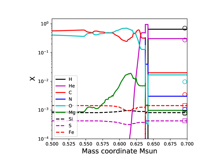
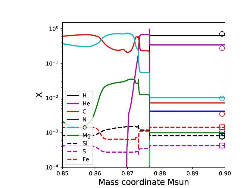
Figure 1: Model abundance (in mass fraction X) profile for the elements H, He, C, N, O, Mg, Si, S and Fe for two AGB stars with initial mass $M$=3M_⊙ (upper panel) and $M$=5M_⊙ (lower panel), and Z=0.02 (Ritter et al., 2018b). The boundary of the AGB envelope is at about M=0.64M_⊙ and M=0.876M_⊙ for the 3M_⊙ and 5M_⊙ models, respectively. As a reference, the initial elemental abundances are reported with empty symbols of the same color of the reference lines (circles and squares are used for elements plotted with continuous lines, and squares for dashed lines).

Moreover, massive stars and CCSNe produced the bulk of O and Mg in stars in the MW disk, as well as relevant quantities of C, N, Si, S, and Fe. For these stellar objects, a substantial amount of the initial mass is lost by stellar winds, but most of the metals are ejected in the final CCSN explosion (e.g., Woosley et al., 2002). A contemporary view, however, is that not all massive stars will successfully explode as CCSN. Depending on the progenitor structure and on details associated with the as yet poorly understood explosion mechanism, not all the material ejected by the SN explosion manages to escape and fall back to the compact central object (e.g., Fryer et al., 2012; Ugliano et al., 2012; Ott et al., 2018; Fryer et al., 2018). In the most extreme cases, all the ejecta fall back and only the winds contribute to the ISM enrichment. Present uncertainties of the CCSN mechanism, however, continue to undermine the efficacy of theoretical simulations (e.g., Fryer et al., 2018; Müller, 2016; Janka et al., 2016; Burrows & Vartanyan, 2021). Direct observations of recent CCSN remnants appear to confirm that a large variety of ejecta and energetic configurations are indeed possible (e.g., Nomoto et al., 2013; Smartt, 2015; Martinez et al., 2022). It is unlikely that these different possibilities observed in recent CCSNe are mostly due to physics mechanisms seldom included in stellar model sets like rotation (e.g., Heger et al., 2000; Hirschi et al., 2005; Limongi & Chieffi, 2018) and/or more exotic types of supernova explosion like Pair-Instability Supernovae (e.g., Heger & Woosley, 2002; Kozyreva et al., 2014; Takahashi et al., 2018; Goswami et al., 2022), which are expected to be more relevant for stars at low metallicity. The start of a successful or weaker CCSN explosion shown by the observations is instead most likely affected by the details of the stellar progenitor structure and by its interaction with the forming SN shock (Wongwathanarat et al., 2013; Burrows & Vartanyan, 2021; Varma et al., 2023). For recent studies of the nucleosynthesis in massive stars and CCSNe, we refer to e.g., Pignatari et al. (2016), Sukhbold et al. (2016), Ritter et al. (2018b), Limongi & Chieffi (2018), Curtis et al. (2019), Ebinger et al. (2020), Andrews et al. (2020).

Figure 2 shows the abundance profile of the CCSN ejecta of 15M_⊙, 20M_⊙ and 25M_⊙ models by Ritter et al. (2018b). The 15M_⊙ model shows the most classical onion-layer structure (top panel, Figure 2). The explosive Si-burning and explosive O-burning ejecta are squeezed within the inner mass range 0.2-0.3 M_⊙, producing a peak of Fe (originally made as ⁵⁶Ni, which will decay to ⁵⁶Fe powering the peak of the CCSN lightcurve) and a peak of Si and S, respectively. Moving outward (toward the right in the plot), we find the O-rich and Mg-rich extended ashes of pre-supernova C fusion. The next large He-rich region represents the remains of the He-shell, with enrichment in C and O and the signature of explosive He-burning at the bottom (i.e., the Mg peak and a small Si peak at M=3.1M_⊙). At the top of the He-ashes are the remains of the pre-supernova H-shell, where C and O are consumed to make N. Finally, at the right edge of the plot is the H-rich envelope of the star. Such a structure is common and is shared across several sets of one-dimensional CCSN models (e.g., Woosley & Weaver, 1995; Thielemann et al., 1996).

The 20M_⊙ and 25M_⊙ models show a fundamental difference when compared to the 15M_⊙ model. In the 20M_⊙ model case the explosive Si-burning layers are not ejected, and only a fraction of the explosive O-burning escapes the gravitational bounds of the central compact object. Such a model represents what is dubbed a faint supernova (e.g., Heger et al., 2003; Nomoto et al., 2013), where the same nucleosynthesis as that in the 15M_⊙ star produces very different Si/Fe or Mg/Si ratios in the ejecta, due to the different outcome of the CCSN explosion.

Faint CCSNe are considered potential sources of the peculiar stellar abundances observed in a number of old metal-poor stars, such as the so-called CEMP-no stars, i,e. carbon-enhanced, metal-poor stars with no enrichment of heavy elements (e.g., Beers & Christlieb, 2005; Ishigaki et al., 2014; Bonifacio et al., 2015; Maeder et al., 2015; Lee et al., 2019; Zepeda et al., 2023, and references therein). In fact, the most Fe-poor star known, SMSS J031300.36-670839.3, was proposed to carry the unique abundance signature of an Fe-poor faint CCSNe (Keller et al., 2014; Bessell et al., 2015; Nordlander et al., 2017). Wehmeyer et al. (2019) discussed the contribution of faint CCSNe to explain the observed scatter of heavy element r-process enrichments with respect to iron in the early Galaxy. Those GCE simulations assume as main r-process sources neutron-star mergers and neutron star- black hole mergers, where black holes are considered as the remnants of faint CCSNe. Nevertheless, the contribution of faint CCSNe to GCE is not well defined. This applies also to the MW disk, although SN lightcurves and remnants of recent faint CCSNe explosions are observed (e.g., Nomoto et al., 2013).

In Figure 2, the 25M_⊙ model exhibits an even more extreme case of faint supernovae, where the whole explosive O-burning layers are not ejected. Even so, depending on the CCSN explosion energy and the progenitor structure, a more or less effective explosive He-burning can produce Mg, Si, and even S in relevant quantities (see mass coordinates M = 5M_⊙ and M = 7-7.5M_⊙ for the 20M_⊙ and 25M_⊙ models, in the central and bottom panels in Figure 2, respectively). Analysis of the presence of a C/Si zone at the bottom of the He shell during the CCSN explosion explains the anomalous abundance signature measured in C-rich presolar grains made in CCSNe (Pignatari et al., 2013). In terms of contribution to the total CCSN yields, the explosive He-burning contribution to Mg, Si and S is typically small compared to that of the explosive Si- and O-burning ejecta. Yet, in the case of faint CCSNe, the contribution of the external layers to the total ejecta of these elements can be relevant. The relative contribution between standard CCSNe and faint CCSNe to the GCE of the Milky Way disk and of the solar neighbourhood is not known. We will return to this point in the next section.

There are additional major uncertainties that need to be considered. According to basic stellar evolution principles, and considering the nuclear reactions involved, O and Mg are produced and ejected in the same CCSN layers and therefore ought to scale nearly perfectly to each other in their GCE history. Pre-supernova He-burning makes O via the ¹²C($\alpha$,$\gamma$)¹⁶O reaction, together with a small amount of Mg. During C-fusion, O is left mostly unchanged whereas Mg is made efficiently in the form of ²⁴Mg via the ²⁰Ne($\alpha$,$\gamma$)²⁴Mg reaction. In the following evolutionary stage, O-fusion destroys both O and Mg. Therefore, the Mg/O ratio should be quite similar in the C-burning ashes of all CCSNe (e.g., Arnett & Thielemann, 1985; Thielemann & Arnett, 1985; Chieffi et al., 1998). Then again, explosive He-burning decouples O and Mg, where O feeds the production of Mg (and eventually Si and S) via a sequence of $\alpha$-capture reactions (Pignatari et al., 2013).

In a similar way, the production of Si and S is generally expected to be connected, since these elements are produced together by the two main O-burning fusion channels in the form of their stable isotopes ²⁸Si and ³²S, respectively (e.g., Thielemann & Arnett, 1985). It is apparent that abundance profiles of Si and S, however, change significantly in the models shown in Figure 2. In the C-burning ashes of the 20 M_⊙ and 25 M_⊙ models, nuclear reactions have already started to make Si, while S is only marginally modified. In these CCSN explosions, it is evident that the C-ashes and eventually explosive He-burning products shape the S/Si ratio in the yields. In the 15M_⊙ model, we find instead that the ratio S/Si$<$1 typical of O-burning is shown only in the small region shaped by the explosive O-burning (M$\sim$1.6M_⊙). The C-ashes instead show a ratio S/Si$>$1, with both Si and S being more than 10$\%$ in mass fraction. This is the signature of the C-O shell merger, which occurs during the pre-SN evolution of the star and allows for the pollution of the C shell with O-burning products, with a signature quite different compared to pure O-burning material.

The study of the interaction between the convective C-shell and O shell up to a complete C-O shell mergers was considered in previous nucleosynthesis studies (Rauscher et al., 2002; Ritter et al., 2018a; Clarkson et al., 2018). In these conditions, the predictive power of one-dimensional models is limited and multi-dimensional hydrodynamics simulations are required (e.g., Meakin & Arnett, 2006; Cristini et al., 2017; Andrassy et al., 2020; Clarkson & Herwig, 2020). The potential relevance of these events in triggering the asymmetries in the progenitor structure favouring successful CCSN explosions is also a matter of debate (e.g., Janka, 2017; Ott et al., 2018). For the purpose of our analysis, this implies that some scatter can be expected for the S/Si ratio in CCSN ejecta. The same scatter could be possibly visible in stellar observations, if observational uncertainties are small enough (Chen et al., 2002; Reddy et al., 2003, 2006). Therefore, the common assumption made in forward simulations of planetary formation, where the initial Si and S abundances scale together with respect to the solar abundances (e.g., Bitsch & Battistini, 2020) needs to be carefully checked against the spectroscopic data from the stellar host, or with GCE simulations, when S observations are not available.

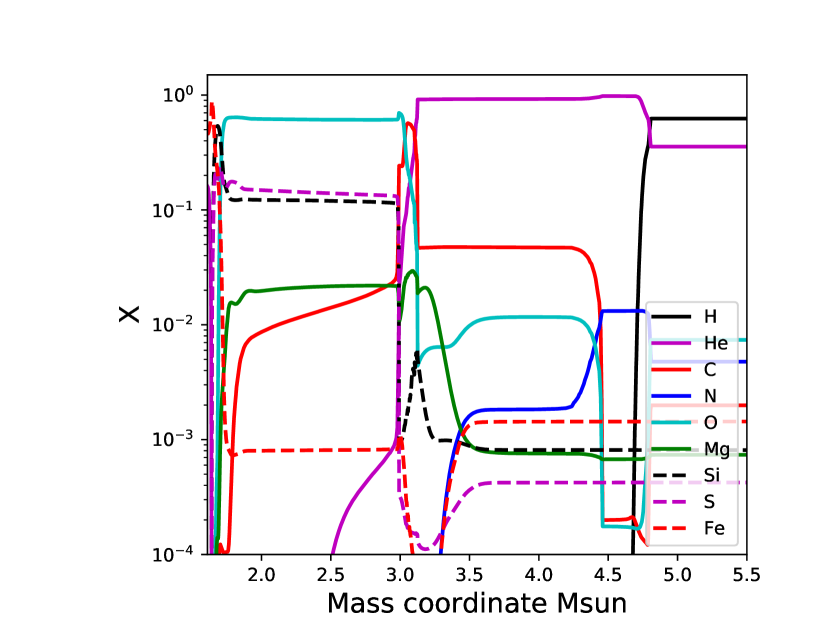
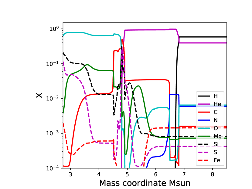
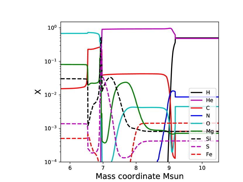
Figure 2: Abundance (in mass fraction X) profiles for the elements H, He, C, N, O, Mg, Si, S, and Fe for CCSN models from massive-star progenitors with initial mass M=15 M_⊙ (upper panel), M=20 M_⊙ (central panel) and M=25 M_⊙ (lower panel) and Z=0.02 (Ritter et al., 2018b). The deepest ejecta are shown to the left, while the H-rich envelope is located to the right of the plots. Material that forms the compact central neutron star directly, or that will afterwards fall back onto it, is not considered.

The last stellar source we consider here are Supernovae Type-Ia (SNIa) which are responsible for the synthesis of the bulk of Fe measured in stars in the Milky Way disk, as well as a significant fraction of Si and S. Uncertainties surround the relative importance of the single-degenerate scenario (where the SNIa explosion is triggered by accretion of material on a CO-WD reaching the Chandrasekhar mass) with respect to the double-degenerate scenario (where the SNIa explosion is triggered by the merger of two CO-WDs) in the SNIa population of galaxies at present. (Hillebrandt et al., 2013). A complementary matter of discussion is the relative contributions of SNIa explosions from Chandrasekhar-mass progenitors and sub-Chandrasekhar-mass explosions, where also in the single-degenerate scenario a SNIa may explode before reaching 1.44M_⊙. To explain the GCE of the ratio [Mn/Fe] in the MW disk, Kobayashi et al. (2020a), Seitenzahl et al. (2013) and Eitner et al. (2020) concluded that only 75$\%$, 50$\%$ and 25$\%$ of all the SNIa population should be from Chandrasekhar-mass progenitors, respectively. On the other hand, based on observational surveys of early-type galaxies Woods & Gilfanov (2013) and Johansson et al. (2016) determined that only a few per cent of all SNIa should be from Chandrasekhar-mass progenitors. These two conclusions are obviously at odds with one another and warrant further study. Finally, it is also important to note that from a study of 407 SNIa in older massive Red-Sequence galaxies and younger less massive Blue-Cloud galaxies, Hakobyan et al. (2020) showed that about one-third of all SNIa events are peculiar, possibly related to the contribution from double-degenerate WD mergers, and that the diversity of SNIa progenitors may also be due to the age of the progenitor. Such a phenomenological diversity is difficult to capture within GCE simulations, but it will need to be considered in the future.

Figure 3 shows the abundances normalized to their solar values for the elements between Mg and Fe for SNIa models computed with the same initial ²²Ne abundance equivalent to a metallicity of Z=0.014 (Keegans et al., 2023). The three models correspond to explosions of different masses of WD: 1.37 M_⊙ (Townsley et al., 2016), 1 M_⊙ (Shen et al., 2018) and 0.8 M_⊙ (Miles et al., 2019). For the elements around Fe, the 1.37 M_⊙ and 1 M_⊙ progenitors produce very similar distributions, while the lowest mass progenitor produces far less of these in absolute abundances. For Fe itself, the production factor in the low-mass case is almost an order of magnitude lower than in the other two models. On the other hand, for the elements of interest in our discussion here, Si and S production factors are similar in the figure, and show only minor variations between the different models. This is because Si and S are typically produced in the same explosive conditions, and they are ejected together in the SNIa ejecta. This makes their production less sensitive to the relevant stellar uncertainties. Note that the contribution timescale (or delay-time) to GCE from different types of SNIa explosions may change depending on how the explosion was triggered in the stellar progenitors. Standard Chandrasekhar-mass SNIa accreting H will have a long delay-time (in the order of 1 Gyr, see e.g., Ruiter et al., 2009). This would be the case for the models by Townsley et al. (2016), shown in Figure 3. Sub-Chandrasekhar-mass SNIa accreting He from a WD companion have a comparably long delay-time to the standard Chandrasekhar-mass SNIa (e.g., Gronow et al., 2021a). This would be the scenario compatible with the Shen et al. (2018) and the Miles et al. (2019) models shown in Figure 3. On the other hand, in case He would have been accreted by a He-burning star, the delay-time of Sub-Chandrasekhar-mass SNIa would be much shorter (in the order of few hundred million years, see e.g., Ruiter et al., 2014). However, in the present context where different types of SNIa produce yields with similar S/Si abundance ratios, the GCE impact of varying the delay-time for different SNIa progenitors would be marginal.

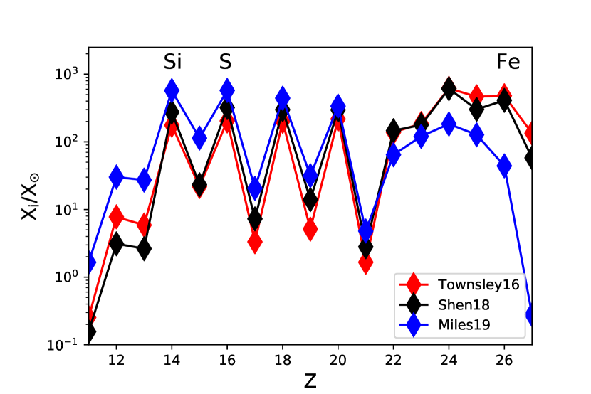
Figure 3: Elemental abundances (normalized to the solar values) in the mass region between Si and Fe for the SNIa models by Townsley et al. (2016), Shen et al. (2018) and Miles et al. (2019), with progenitor masses 1.37M_⊙, 1M_⊙ and 0.8M_⊙, respectively. Yields are calculated by Keegans et al. (2023).

3 GCE Models and simulations

To explore the GCE of the solar neighbourhood we produced a set of 198 models; we use the OMEGA GCE code (One-zone Model for the Evolution of GAlaxies Côté et al., 2017a) to calculate elemental abundance ratios in the ISM for several choices of stellar-yield sets and of the contribution from faint CCSNe yields. OMEGA has also an option for including any number of extra enrichment sources, in addition to the mass- and metallicity-dependent yields from AGB stars, massive stars, CCSNe, and SNe Ia described above which are included by default in the code. The OMEGA code, the simple stellar population (SSP) model SYGMA (Stellar Yields for Galactic Modeling Applications Ritter et al., 2018c), and the STELLAB (STELLar ABundances) module used to plot the observational data are all part of the publicly available NuGrid chemical evolution framework. Here we give a brief description of the OMEGA code.

The evolution of the mass of the gas-reservoir in the Galaxy as a function of time can be expressed in terms of the gas inflow rate $\dot{M}_{\text{inflow}}(t)$, the rate at which gas is ejected from stars $\dot{M}_{\text{ej}}(t)$, the star-formation rate (SFR; $\dot{M}_{\star}(t)$), and the outflow rate of gas from the galaxy $\dot{M}_{\text{outflow}}(t)$ (e.g., Tinsley 1980; Gibson et al. 2003; Matteucci 2021), where

$$\dot{M}_{\text{gas}}(t)=\dot{M}_{\text{inflow}}(t)+\dot{M}_{\text{ej}}(t)-\dot{M}_{\star}(t)-\dot{M}_{\text{outflow}}(t).$$ (1)

The gas ejected by stars is assumed to mix instantaneously with the ISM, so that the metallicity of the gas-reservoir is always homogeneously distributed, as is the case for all one-zone GCE models. OMEGA also includes a simple treatment of galactic inflows and outflows. Since stellar feedback is assumed to drive the gas outflows, then

$$\dot{M}_{\text{outflow}}(t)=\eta\dot{M}_{\star}(t),$$ (2)

where the mass-loading factor $\eta$ is a free parameter controlling the magnitude of the gas outflow (e.g., Murray et al. 2005; Muratov et al. 2015). The inflow of primordial matter is a catalyst for star-formation in the Galaxy, however OMEGA uses the star-formation history to determine the SFR rather than the inflow rate. For further details regarding the treatment of galactic inflows in OMEGA we refer the reader to Côté et al. (2017a).

At each timestep, OMEGA creates a single stellar population (SSP) with a mass proportional to the SFR at that time, which is proportional to the total mass of gas in the Galaxy following the Kennicutt-Schmidt law (Schmidt, 1959; Kennicutt, 1998):

$$\dot{M}_{\star}(t)=f_{\star}\dot{M}_{\text{gas}}(t),$$ (3)

where $f_{\star}=\epsilon_{\star}/\tau_{\star}$ is a combination of the dimensionless star-formation efficiency $\epsilon_{\star}$ and the star-formation timescale $\tau_{\star}$. All stars in a given SSP have the same initial metallicity - that of the gas-reservoir - since they are all assumed to have formed from the same parent gas cloud. At each timestep, the SYGMA code calculates the combined integrated yields from all the SSPs that are currently in the Galaxy. However, each star in an SSP will eject material at different times according to the delay-time distribution (DTD) function of the specific progenitor. For a galaxy with $j$ SSPs at time $t$, the combined integrated yield returned by SYGMA is given by

$$\dot{M}_{\mathrm{ej}}(t)=\sum_{j}\dot{M}_{\mathrm{ej}}\left(M_{j},Z_{j},t-t_{j}\right),$$ (4)

where $Z_{j}$ and $M_{j}$ are the initial mass and metallicity of the $j^{\text{th}}$ SSP that was born at time $t_{j}$. Significantly for the present study, if an extra source (e.g., faint CCSNe) is added to SYGMA, then a DTD must also be assigned to it, in addition to specifying the yields, the number of events per M_⊙, and the mass ejected per event.

Here, we assume that a fraction of massive stars $f_{\text{faint}}$ with initial mass $M$ above a given mass threshold $M_{\text{min}}$ will explode as faint CCSNe, rather than wholly as regular CCSNe. At the moment, it is still unclear if faint CCSNe have a significant impact on the GCE. Indeed, their presence may be hidden in the variations due to the uncertainties affecting the yields of CCSNe. Although previous GCE studies adopted various CCSN yields from the literature, they might have mitigated faint CCSN uncertainties by varying other parameters such as the slope of the IMF, the range of stellar masses contributing to the nucleosynthesis, the star-formation efficiency, and the strength of large-scale gas flows (e.g., Gibson, 1997; Romano et al., 2010; Mollá et al., 2015; Côté et al., 2017b; Philcox et al., 2018). Given the lack of constraints for the value of $f_{\text{faint}}$, we consider values between 0 and 1 in order to fully explore the potential impact of faint CCSNe.

Since both faint and regular CCSNe share the same type of progenitors, the only defining factor between the two types of explosion mechanisms are their yields. Therefore, for M>M${}_{\text{min}}$ we make the simplification that faint and regular CCSNe occur at the same frequency in the Galaxy, but we apply a $f_{\text{faint}}$ correction factor to the yields of faint CCSNe, and a $1-f_{\text{faint}}$ correction factor to yields of the latter. We make no modifications to the yields of CCSNe that result from massive-star progenitors with M<$M_{\text{min}}$. The models considered for this work are summarized in Table 1. The adopted name scheme is o<yield$\_$identifier><faintSN$\_$model><faintSN$\_$weight>. The term $M_{\rm up}$ represents the mass of the most massive stars that can contribute to the GCE. All stars with an initial mass above $M_{\rm up}$ are assumed to directly collapse into a black hole without any ejecta.

With regards to stellar yields, for AGB stars the oK06, oR18, oR18d and oR18h sets use Ritter et al. (2018b), while the oK10 and oL18 models use the yields by Karakas (2010). The CCSN yields by Kobayashi et al. (2006) are adopted in the oK06 and oK10 models, and non-rotating massive-star yields by Limongi & Chieffi (2018) are adopted in the oL18 models. The remaining sets of models use different yield setups by Ritter et al. (2018b). In particular, oR18d, oR18 and oR18h use the same AGB stellar yields, but oR18d use the CCSN models with a delayed explosion setup (Fryer et al., 2012), oR18h is the same as oR18d but the 12M_⊙ yields are not included, while for oR18 CCSN models adopt a classical mass cut defined by the electron fraction ($Y_{e}$) jump in the progenitor structure (Côté et al., 2017b). For all GCE models, the OMEGA default W7 SNIa yields by Iwamoto et al. (1999) are used for all metallicities. Notice that within our GCE platform there are multiple sets of SNIa yields available (e.g., Lach et al., 2020; Gronow et al., 2021b). However, since for the elements considered in this study the impact of using different SNIa yields is much smaller compared to CCSN yields, we decided to not modify the default setup for the models discussed here.

For each GCE model setup described above, a number of models are generated with five faint CCSN weighting factors of 10$\%$, 25$\%$, 50$\%$, 75$\%$ and 100$\%$ respectively, and two types of faint CCSNe: the stellar model of 20 M_⊙ by Ritter et al. (2018b) (model m20, Figure 2, central panel), and 25 M_⊙ (model m25, Figure 2, lower panel). The additional contribution of faint CCSNe is considered for stellar progenitor masses larger than $M_{\rm min}$ = 15M_⊙. The weighting factor mentioned above provides the relative contribution of faint CCSNe compared to default SNe yields for the mass range M > $M_{\rm min}$.

Analogous GCE model sets are generated considering three different $M_{\rm up}$: 20 M_⊙, 40 M_⊙ and 100 M_⊙ as the value of M_up is uncertain and it is still a matter of debate. While $M_{\rm up}$ = 40 M_⊙ and 100 M_⊙ are more typical choices, we also considered in our calculations the lower value at 20M_⊙, which would be more consistent with observations from CCSN remnants and their progenitors (e.g., Smartt, 2015; Davies & Beasor, 2018). Such a lack of CCSNe from massive stars with initial mass M $\gtrsim$ 20 M_⊙ also seems to be plausible for stellar simulations, where a relevant population of massive stars with initial mass larger than 20 M_⊙ may fail to explode (e.g., Sukhbold et al., 2016; Fryer et al., 2018), and it is indepently confirmed by direct element observations of late-time supernova spectra (e.g., Jerkstrand et al., 2014; Jerkstrand et al., 2015; Silverman et al., 2017, and references therein).

Table 1: Summary of the GCE models used in this work with their properties: name (used in the text), stellar yields set identifier (see the details in the text), faint CCSN model if included, and its frequency with respect to the default yields. The extra sources "m20" and "m25" correspond to the M=20 M_⊙ and the M=25 M_⊙ faint CCSN models by Ritter et al. (2018b), respectively (Figure 2, central panel and lower panel). The last column provides the upper limit of stellar masses contributing to the GCE (in solar masses). The models name are designed as follows: o<yield$\_$identifier><faintSN$\_$model><faintSN$\_$weight>, where the initial o stands for OMEGA.

yield$\_$identifier	faintSN$\_$model	faintSN$\_$weight	Mup (M⊙)
K06	-	no,	20, 40, 100
	m20, m25	f0p10, f0p25, f0p50,	20, 40, 100
	m20, m25	f0p75, f1p00	20, 40, 100
K10	-	no,	20, 40, 100
	m20, m25	f0p10, f0p25, f0p50,	20, 40, 100
	m20, m25	f0p75, f1p00	20, 40, 100
R18	-	no,	20, 40, 100
	m20, m25	f0p10, f0p25, f0p50,	20, 40, 100
	m20, m25	f0p75, f1p00	20, 40, 100
R18d	-	no,	20, 40, 100
	m20, m25	f0p10, f0p25, f0p50,	20, 40, 100
	m20, m25	f0p75, f1p00	20, 40, 100
R18h	-	no,	20, 40, 100
	m20, m25	f0p10, f0p25, f0p50,	20, 40, 100
	m20, m25	f0p75, f1p00	20, 40, 100
L18	-	no,	20, 40, 100
	m20, m25	f0p10, f0p25, f0p50,	20, 40, 100
	m20, m25	f0p75, f1p00	20, 40, 100

That the chemical evolution of the solar neighbourhood is complex and a challenging task for GCE, is an understatement (e.g., Goswami & Prantzos, 2000; Kobayashi et al., 2011; Mollá et al., 2015; Prantzos et al., 2018; Kobayashi et al., 2020b; Prantzos et al., 2023). This is because stars that are observed within a few hundred parsecs from the Sun may have formed from material with radically different chemical evolution histories from one another and from our star. In fact, the observed [Fe/H] varies by about an order of magnitude and some stars may have formed after the Sun, or billions of years earlier and shortly after the formation of the Galaxy (e.g., HD140283 Siqueira-Mello et al., 2015). This variety should be taken into account, because the relevance of different stellar sources varies during the galactic evolution timescale (e.g., Matteucci & Greggio, 1986). Stellar ages of nearby stars can be derived with a precision of about 1 billion years (e.g., Nissen et al., 2020). We emphasize that the age of the star needs to be considered together with the stellar abundances in order to fully understand the elemental composition directly observed using spectroscopic data, and that can only be inferred (e.g., Spina et al., 2016).

As an example, Figure 4 shows the evolution with [Fe/H] of the elements in model oK06no along with some reference evolution timescales. Model oK06no provides a good match to the solar abundances for the elements considered at the time when the Sun formed (8.7 Gyr). The predicted [Fe/H] is about 10$\%$ higher than solar. Carbon (mostly made by AGB stars) and O (mostly made by massive stars) are both about 60$\%$ too low. The elements N, Mg, and S are reproduced within 10$\%$ for solar material, while Si (made by both massive stars and SNIa) is about 20$\%$ higher. However, this same model, when considering both the chemical enrichment and evolution timescale, may not be appropriate to use for another star, even one with solar metallicity. We will use the same four reference GCE timescales shown in Figure 4 (1.0, 3.1, 8.7, and 12.0 Gyr) in the next section, to also analyze the evolution curves of elemental ratios with respect to time.

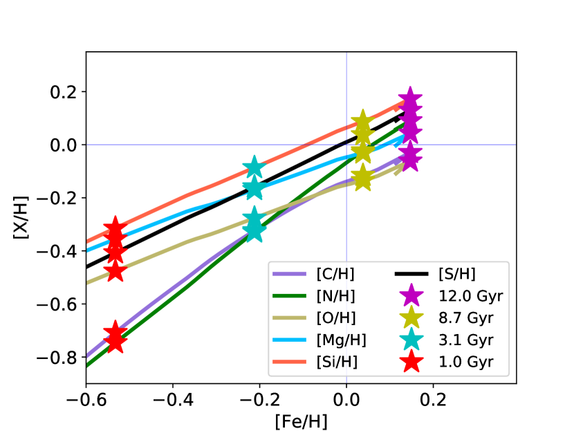
Figure 4: The evolution of the elements of interest with [Fe/H] for the model oK06no (see Table 1 for the model name explanation). Stars of different colors represent evolution times from the beginning of the simulation. The time 8.7 Gyr corresponds to the formation of the Sun.

4 Stellar observation samples and solar abundances

Figure 5 shows the abundances from two different stellar samples from the galactic disk by Reddy et al. (2003) and Reddy et al. (2006) (R03, R06) and Suárez-Andrés et al. (2018) (S18), together with their reference solar ratios. No scaling or normalization has been applied to the C/O and Mg/Si ratios. The two observed distributions exhibit clear discrepancies, where the S18 data have on average both higher C/O and Mg/Si ratios. This difference also appears in the solar abundances used in these surveys, with the S18 C/O and Mg/Si being factors of 1.38 and 1.29 higher than those of R03 and R06, respectively. Figure 5 also plots C/O and Mg/Si ratios from several other solar chemical composition studies. The C/O values range by a factor of two, from 0.83 (Delgado Mena et al., 2010, D10 HARPS) to 0.43 (Anders & Grevesse, 1989, AG89). The Mg/Si ratios are also scattered, varying between 0.83 (Reddy et al., 2003, based on their own solar analysis), and 1.23 (Asplund et al., 2009, A09). These variations indicate that solar abundance differences are not limited to the two stellar surveys employed in our investigation. The details of these abundance determinations can be found in the survey papers. We report below some general remarks about observational uncertainties.

4.1 Comparing Results from the Abundance Surveys Considered Here

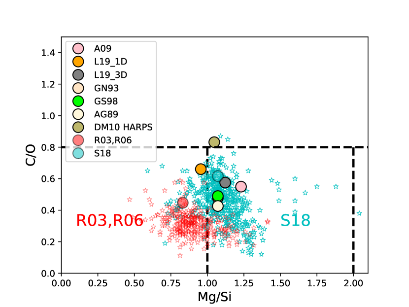
Figure 5: The C/O and Mg/Si ratios for stars by Reddy et al. (2003) and Reddy et al. (2006) (R03 and R06, red stars) and Suárez-Andrés et al. (2018) (S18, cyan stars). The solar ratios used as reference in the two papers are reported, together with a collection of other solar abundances from: Asplund et al. (2009) (A09), Lodders (2019) using 1D and 3D models for the solar atmosphere (L19$\_1$D and L19$\_$3D, respectively), Grevesse & Noels (1993) (GN93), Grevesse & Sauval (1998) (GS98), Anders & Grevesse (1989) (AG89) and the solar abundances measured using HARPS (Delgado Mena et al., 2010) (D10 HARPS). Ratios discussed by Bond et al. (2010) as relevant to the chemistry and dynamics of rocky planets are also reported as black-dashed lines.

Some of the apparent clashes in Figure 5 between the C/O and Mg/Si ratios of R03, R06 and S18 can be alleviated by a normalisation to the solar abundances derived with the same analysis setup. In this way, it is possible to remove at least some of systematic uncertainties. In Figure 6, we report the same stellar ratios shown in Figure 5, but in logarithmic notation and normalized to their respective (and different) solar reference ratios. Because of these, the two stellar samples show a much better overlap compared to Figure 5. The [C/O] ranges are similar, and the [Mg/Si] is also consistent (albeit with significantly more scatter), when excluding outliers with [C/O] $\lesssim$ $-$0.5 and [Mg/Si]$\lesssim$ $-$0.2. The set by S18 is concentrated around the solar values or slightly higher, while R03 and R06 data are more scattered toward larger Mg/Si values, up to about 0.2 dex. The larger ranges of both C/O and Mg/Si in the R03 and R06 sample combined reveals that the two surveys may not draw their targets from the same Galactic metallicity/kinematic samples. Indeed, from Figure 6 we can see that the high Mg/Si-signature is mostly given by R06 stars, which are mostly thick-disk stars. The R03 stars are instead in better agreement with the S18 scatter.

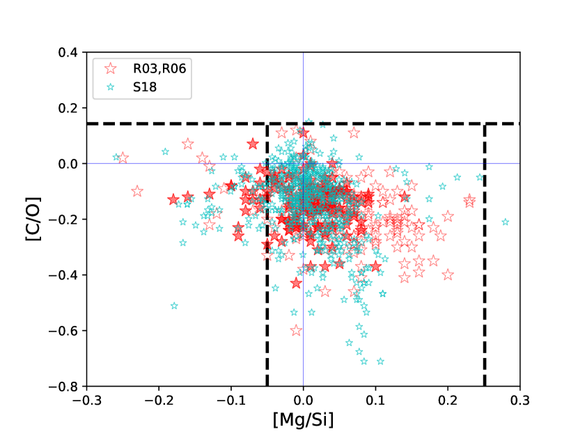
Figure 6: The [C/O] and [Mg/Si] ratios for stellar data by R03 and R06 (full and open red stars, respectively) and S18 (cyan stars). The indicative abundance errors reported by R03 and R06 are in the order of $\pm$0.2 dex for [C/O] and $\pm$0.1 dex for [Mg/Si]. The average errors reported by S18 are about a factor of two smaller. The same reference lines of Figure 5 are reported, normalized to solar (L19$\_$3D by Lodders (2019)). The reference solar L19$\_$3D is very close to the solar of S18 (see Figure 5 for comparison).

The abundance surveys considered here were conducted using similar methods. They both used model atmospheres from the ATLAS grid (Kurucz, 2011, 2018) and performed equivalent width and synthetic spectrum analyses with the current versions of the same LTE plane-parallel code (Sneden, 1973). On the other hand, R03, R06 and S18 surveys have different selection functions. The HARPS S18 sample is a subset of $\sim$500 stars from the HARPS Adibekyan et al. (2012) sample, who chose their objects based on suitability for radial velocity surveys (slowly rotating FGK stars without chromospheric activity); the R06 sample was primarily selected from kinematically thick Galactic disk but within a given distance and R03 mostly includes selected stars from the kinematically thin Galactic disk. Different software was employed to measure equivalent widths, but the basic procedure is straightforward and accurate for unblended spectral lines. The two surveys differ either in the choice of species for study or in the selection of the individual spectral features. Here we briefly comment on each element. The cited papers describe the details of the analyses and discuss the uncertainties.

Carbon: R03 and R06 employed six high-excitation C i lines, using transition probabilities in agreement with those currently recommended by the curated NIST Atomic Spectra Database. S18 adopted C abundances derived from the CH molecular G-band by Suárez-Andrés et al. (2017). Both C i and CH can yield reliable C abundances in solar-type stars, but the response of these two species to variations in atmospheric temperature and gravity parameters is dissimilar. This could justify the existence of relevant differences in the derived abundances when using these two observational sources. For additional comments on transitions and references to solar C studies see Asplund et al. (2021). Note that Delgado Mena et al. (2021) re-derived the C abundance for the HARPS sample (S18) using atomic lines C i (like R03 and R06): they derived typically larger C abundances compared to S18, especially for cool and metal-poor stars. Therefore, the same [C/O] variation seen in e.g., Figure 5 for S18 with respect to R03 and R06 would have been comparable or larger if we would have used Delgado Mena et al. (2021) data instead of S18.

Oxygen: No molecular species are available in the optical spectral regime, and there are very few detectable O i lines. R03 and R06 derived O abundances exclusively from the high-excitation O I 7700 Å triplet lines. S18 adopted instead their abundances from Bertran de Lis et al. (2015), who employed a unique combination of the [O i] 6300 Å ground-state line and a high-excitation O i line at 6158 Å. The high-excitation lines of this species have long been known to exhibit departures from local thermodynamic equilibrium (Caffau et al., 2008; Asplund et al., 2021). The 6300 Å[O i] line is very weak in solar-type stars, and is significantly blended with a Ni i transition (Allende Prieto et al., 2001). Such concerns, along with different transition choices in the two surveys, serve as cautionary notes.

Magnesium: Mg i lines are the only reliable Mg abundance sources. MgH lines are detectable near 5000 Å, but they are weak and very blended with strong atomic lines and C₂ molecular features. There are relatively few available Mg i transitions, and those well known ones are often very strong. Many of the usually employed lines (4730.00 Å, 4730.30 Å, the Fraunhofer "b" triplet, 5528 Å, and 5711.10 Å) are saturated in the solar spectrum: log($EW/\lambda$) > -4.8 (Moore et al., 1966). Therefore, the derived Mg abundances depend on atomic damping parameters and on the adopted atmosphere conditions in the outer photospheric model. R03 and R06 selected three Mg i lines, two of which are weak enough to be relatively sensitive to Mg abundances. S18 adopted the abundances from Adibekyan et al. (2012), who in turn used the line lists of Neves et al. (2009) for their study of three Mg i lines, with just one of them being in common with R03 and R06. The log($gf$) values are generally in accord with the values recommended by NIST, however we note that the NIST laboratory sources are decades old and would benefit from modern re-analysis. Finally, a carefully developed line list from 4750-8950 Å has been constructed by the Gaia-ESO consortium (Heiter et al., 2021). Their transition probabilities for Mg i are in accord with those used the the two surveys of interest here.

Silicon: A rich Si i spectrum is available in the optical spectra of solar-type stars, but transition probabilities have not been subjected to comprehensive laboratory analyses in recent decades. The R03, R06 and S18 (again, based on the earlier papers by Adibekyan et al. (2012) and Neves et al. (2009)) used 7 and 18 lines; their log($gf$) scales agree reasonably well within 0.0 $\pm$ 0.07 dex, for the 5 lines in common. However, the line-to-line scatter between Neves et al. (2009) and NIST (0.21 dex) and between Neves et al. (2009) and Heiter et al. (2021) (0.14 dex) would be eminently more useful if it was not so large, and deserves to be re-investigated.

Our brief summary of line list issues in the two surveys should be viewed as illustrative; such questions need to be kept in mind for all abundance data sets. Another fundamental problem that needs to be addressed in the near future is the lack of recent comprehensive investigations by the atomic physics community of transition probabilities. With current data it is reasonable to hope for survey-to-survey agreement to the $\simeq$0.05 dex level. Deriving abundance uncertainties to $\simeq$0.05 dex remains a future goal.

4.2 Brief Comments on other Surveys

We have concentrated on the R03, R06 and S18 studies because they have extensive abundance data on all four elements of interest for understanding gross planetary characteristics, and used similar analytical procedures. Other groups have made significant contributions to Galactic disk abundance surveys. The $\alpha$ elements as well as C and O have been studied in various surveys at different spectral resolutions in different spectral regions, such as by GALAH (e.g,, Clark et al. 2022, Sharma et al. 2022), and Gaia-ESO (e.g., Kordopatis et al., 2015). Here we call attention to a noteworthy contribution by T. Bensby and collaborators. Figure 7 shows the [Mg/Si] ratios versus [Fe/H] for our main surveys and the 714 star sample of Bensby et al. (2014). These authors used extensive line lists of Mg i and Si i, and transition probabilities from laboratory work and reverse solar analyses, as discussed in Bensby et al. (2003). Inspection of Figure 7 reveals a drift to larger [Mg/Si] values with decreasing [Fe/H]. The addition of the Bensby et al. (2014) sample highlights this trend, which is weaker in R03, R06 and S18. Note that it appears to be independent of Galactic thin-disk, thick-disk, and halo-population memberships.

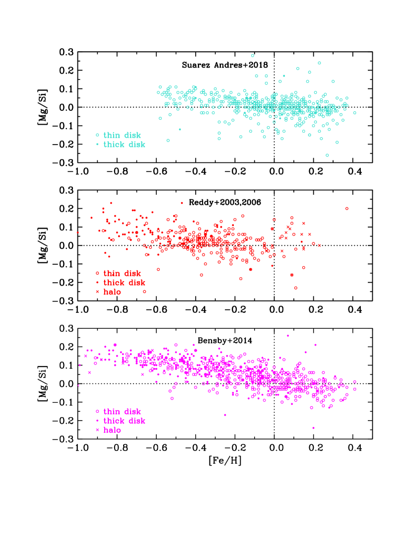
Figure 7: [Mg/Si] abundance ratios as functions of [Fe/H], for S18 (top panel), R03 and R06 (middle panel), and Bensby et al. (2014) (bottom panel). Thin disk, thick disk, and halo stellar populations as defined in the individual papers are shown with different symbols, that are identified in the figure legends.

Bensby et al. (2014) reported O but not C abundances, so their data could not be added into Figure 5. It is worth noting that Bensby & Feltzing (2006) derived [C/O] ratios from a unique forbidden-line combination: [C i] at 8727 Å and [O i] 6300 Å transitions. In general, their [C/O] ratios are $\simeq$0.15 dex higher than those of R03, R06 and S18. The Bensby & Feltzing sample size is relatively small compared to the other samples discussed here, $\simeq$50 stars, and it overlaps with the Bensby et al. (2014) list only for a few stars. In general, a large sample investigation of [C/Fe] ratios from the combination of CH, C₂, C i, [C i], and possibly CO in unevolved disk stars would be an important anchor for all future C abundance studies.

4.3 Astrophysical Implications of C/O and Mg/Si in Local Samples

The stellar samples considered in Figure 5 and Figure 7 show significant star-to-star scatter in [C/O] and [Mg/Si], $\sigma$ $\simeq$ 0.2 dex. As there are systematic dependencies on [Fe/H] and stellar populations that lie beyond observational uncertainties, the origin of the internal dispersion is a matter of debate. Some of the scatter must be observational, as outlined in 4.1 but some of this effect may be an intrinsic property of stars in the solar neighbourhood, which is difficult to quantify with the present observational errors. While, e.g., R03, R06, Bond et al. (2010) and S18 find a significant dispersion of stellar abundances, Bedell et al. (2018) obtain a consistency within 10% for Sun-like stars (the stars in their sample are solar twins with very similar metallicities) within 100 pc. It will be paramount in future work to definitively solve these discrepancies and clarify the diversity in composition of the solar neighbourhood.

In section 5, we will compare GCE simulations with solar-scaled observations, so that the systematic uncertainties discussed here will not directly affect our analysis. However, since the absolute elemental abundances are needed for the simulations of planetary systems, we are highlighting the uncertainties discussed in this section as an issue that will need to be addressed. The variations seen in Figure 5 are a clear source of degeneracy for future planet formation and evolution studies.

For the comparison with GCE simulations, we will only use stellar data by R03 and R06, where all the elemental abundances are provided for the elements discussed in the following sections (i.e., C, N, O, Mg, Si and S). Additionally, this allows us to compare GCE simulations with the abundance dispersion observed by R03 and R06, which is larger and more conservative compared to the results by, e.g., Bedell et al. (2018). We have seen that R06 includes indeed a large number of thick-disk stars. While we can expect that the planet-host stellar samples from e.g., TESS and ARIEL will be biased towards more metal-rich, thin-disk stars, the first observational efforts to homogeneously characterize the physical parameters of planet-host stars in the Ariel Reference Sample (Edwards et al., 2019) show the presence of both thick-disk stars and stars that could dynamically belong to either the thin and thick disks (Magrini et al., 2022). Furthermore, it is expected that a number of thick-disk stars will be discovered hosting planetary systems (e.g., from TESS Kepler-444, Campante et al. 2015, and TOI-561, Weiss et al. 2021). The study of these stars and their planetary systems will be a fundamental benchmark for planet formation and the evolution of planetary systems.

Finally, we note that among the elements considered in this work N is not available in the HARPS data used by S18 and Bedell et al. (2018). However, for a sample of 74 stars Suárez-Andrés et al. (2016) also combined HARPS data for relevant elements to derive the N abundance from the NH band in UVES spectra.

5 Results of the GCE simulations

We now summarize our analysis for the elements of interest discussed in Section § 2, using the GCE models introduced in the previous section. All the plots showing the comparison between GCE model predictions and observations are provided in this section or in Appendix § A.

In Figure 8, selected element ratios are plotted against each other and compared to abundances observed in stars within 150 parsecs by R03 (which comprises mostly thin-disk stars) and R06 (which instead comprises mostly thick-disk stars). This is a similar range of distance to consider for stellar hosts of TESS and ARIEL planetary targets (Edwards et al., 2019; Magrini et al., 2022). Therefore, we may assume that this observational sample is consistent with the abundance variations that merit exploration.

The upper-left panel of Figure 8 is the same diagram shown by Bond et al. (2010) but in logarithmic notation, and including GCE models. In general, only the theoretical GCE curves between the red and the magenta stars (which correspond to a GCE evolution age between 1 Gyr and today, Figure 4), should be considered as representative of the evolution over time of the Milky Way disk. Indeed, the observed properties of the old stellar population of the Milky Way halo are consistent with the first Gyr of active star formation, while to reproduce the age and metallicity distribution of the stars in the Milky Way disk much longer times are required (see e.g, Fenner & Gibson 2003).

The observational scatter of about a factor of 2.5 is obtained for both [C/O] and [Mg/Si]. At time of Sun formation, the models oK06no and oK10no produce [C/O] ratios 0.2 dex and 0.3 dex lower than the solar abundances, respectively. However, they reproduce the ratio observed in the majority of stars, with a [C/O] ratio increasing over time (or with metallicity) until about 5 Gyr ago (Bitsch & Battistini, 2020). After Sun formation, the calculated [C/O] is almost constant. The oR18dno model produces a final solar [C/O] ratio. Between the three GCE models using Ritter et al. (2018b) CCSN sets, the different CCSN explosion parametrizations affect the O production with a variation of the [C/O] ratio by about 0.2 dex. At evolution timescales representative of the MW disk, oL18 models show a solar [C/O] ratio with only marginal variation.

The [Mg/Si] is about 30$\%$ lower than the Sun in oK06no and oK10no, between a factor of 1.8 and 2.2 lower for the R18 models, and sub-solar by a factor of $\sim 1.8$ for oL18no. While the bulk of the stars in the solar neighbourhood have a solar-like or super-solar ratio up to [Mg/Si]$\sim$0.2, the GCE models predict a ratio lower than solar for all the combinations of stellar yields considered. In particular, the largest departure seen in oR18no is mostly due to the contribution of energetic CCSN explosions for the 12M_⊙ and 15M_⊙ models by Ritter et al. (2018b). Note that these results would not have changed by considering a different observational stellar sample, e.g. R03 only without the R06 or the S18 sample (see Figure 6). We also cannot expect one-zone GCE simulations to reproduce the observed [Mg/Si] scatter, since at a given evolution time of the model the result is given by a single data point, not by some statistical distribution. However, the predictions should still be compatible with the bulk of the observed stars. Even by varying the stellar yields - one of the main uncertainty sources of GCE - we do not achieve this result. It is true that GCE uncertainties could play a relevant role in the abundance analysis, and in our single-zone GCE simulations we do not take into account relevant processes like stellar migration and past infall of fresh material in the galactic disk (Matteucci, 2021; Prantzos et al., 2023, and reference therein). However, the impact of such processes should be significantly reduced by studying the evolution of primary elements sharing a similar stellar production. For instance, in the specific case of Mg and Si they are both mostly produced by short-lived massive stars, and these do not have sufficient time to migrate significantly (e.g., Sánchez-Blázquez et al., 2009; Minchev et al., 2014).

Such a result where Mg stellar yields seem to be too low compared to observations (and, to a much lesser extent, Si) are not surprising, and they have been highlighted before in the literature. The artificial Mg and/or Si boosting is a well-known requirement of using e.g., the Woosley & Weaver (1995) CCSN yields (Gibson, 1997). More recently, the same approach is implemented by Spitoni et al. (2021) with Woosley & Weaver (1995) yields, where Mg from CCSNe are boosted up to a factor of seven.

The distribution of the CNO elements is shown in the upper-right panel of Figure 8. Models oR18no and OR18dno show an [N/O] ratio increasing with the evolution time and with [Fe/H]. Yet, we find that they both reach the solar [N/O] ratio too early, more than 4 Gyr before the formation of the Sun. The other models instead reproduce the solar ratio to within 0.1 dex. For oL18no, the [N/O] ratio changes little with galactic time, remaining $40-80\%$ super-solar for the duration of the GCE. Several challenges need to be considered for the GCE of CNO elements and their stable isotopes (e.g., Kobayashi et al., 2020b). The contingent relevance of fast rotating stars (not included in our models) was highlighted by several previous works to reproduce the abundance patterns in the Milky Way (e.g., Chiappini et al., 2006, 2008; Prantzos et al., 2018; Romano et al., 2019). Additionally, Pignatari et al. (2015) discussed the contribution of H-ingestion events in massive stars for the GCE of N (and in particular of the N isotopic ratio), using stellar models consistent with abundance measurements in presolar grains made by CCSNe just before the formation of the Sun.

The predictions for N evolution from our GCE models have problems in reproducing the ratios in the Figure 8, lower-left panel. Contrary to most of the observations, all the GCE models produce super-solar [S/N] ratios, except for the oL18no model, which produces a [S/N] ratio significantly lower than solar, but still does not cover the full observational range down to [S/N]$\sim$-0.5 reached by a large number of stars. Most of the stars indeed exhibit a subsolar elemental ratio, with a scatter of the order of a factor of three. The observed [C/N] scatter is instead at least partially reproduced by most of GCE models, where this ratio decreases with evolution time. Note that this does not have to be the right physical reason for the observed [C/N] scatter. As we mentioned earlier, the N evolution is a well-known challenge for GCE, where standard CCSN models underproduce N compared to observations. Finally, model oK10no shows a smaller variation than the other models within sub-solar [C/N] values around $-$0.3 dex.

In the lower-right panel of Figure 8, stars show an observational scatter larger than a factor of two for both [Mg/O] and [S/Si] ratios. Such a variation is only marginally captured by the GCE models: for both ratios, variations at relevant timescale are in the order of 20$\%$ or less. The oK06no, oK10no and oL18no models reproduce the solar ratios within 0.1 dex, the other models are more consistent with the bulk of stars that are mildly S-rich compared to the Sun, up to [S/Si]$\sim$+0.3. If we consider all the GCE models, it may seem that the observed range of [S/Si] is reproduced. However, if we factor in single GCE models we notice that the [S/Si] variation within the acceptable evolution time frame is less than 0.1 dex. The only exception is oR18hno, where between 1Gyr and today the [S/Si] ratio increases by about 0.2 dex. Still, such an increase is much smaller than the scatter observed in the Milky Way disk. Such a dispersion may, in part, be due to observational uncertainties (Bedell et al., 2018). Chemo-dynamical simulations of the Milky Way disk would be needed to provide a realistic prediction for the expected [S/Si] dispersion (e.g., Thompson et al., 2018), which is beyond the goal of this paper.

Alternatively, as we discussed in Section § 2, this dispersion may instead be an indication that CCSN ejecta are not always dominated by an explosive O-burning signature, but that they vary between different supernova events. We have seen that some variations are obtained between different SNIa explosions (Figure 3), although the progenitor mass does not affect the S/Si ratio in the ejecta very much, and the same can be said for the initial metallicity (e.g., Keegans et al., 2023). Note that according to the nuclear sensitivity study by Parikh et al. (2013), there should be no relevant impact of nuclear uncertainties on the SNIa yields of Si and S.

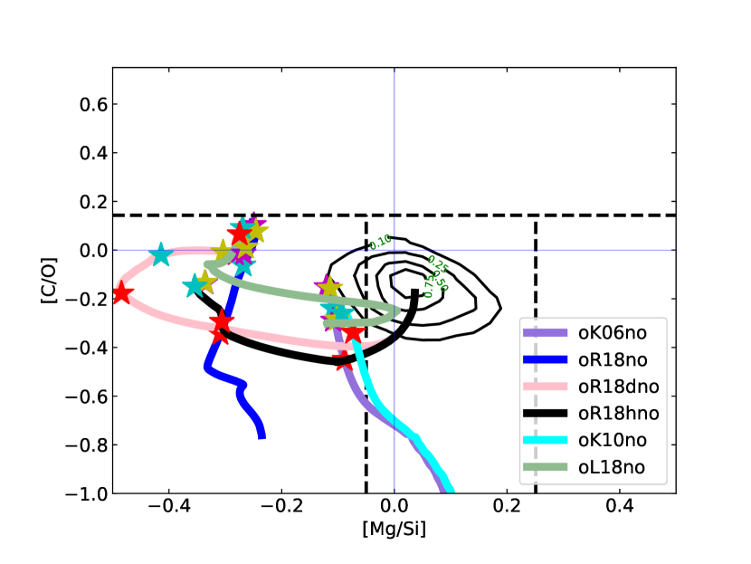
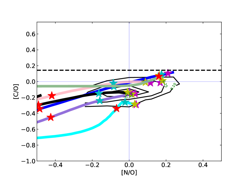
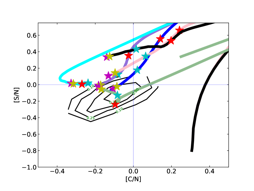
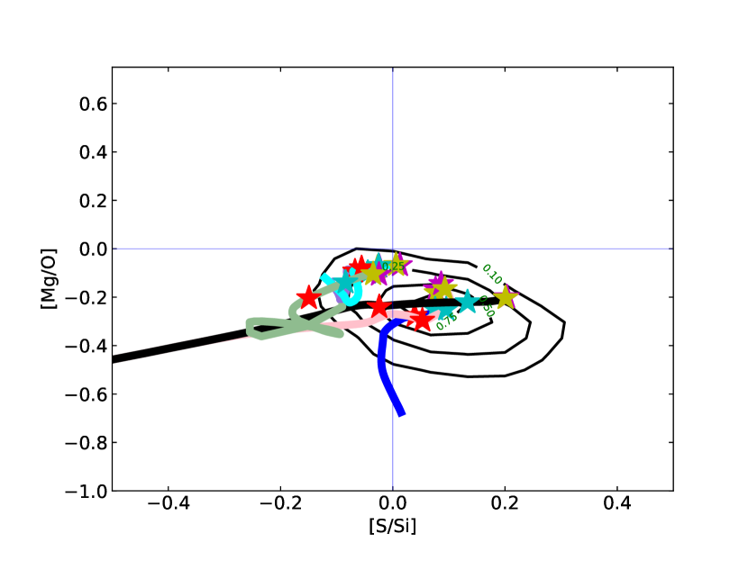
Figure 8: Selected elemental ratios normalized to the solar (L19$\_$3D by Lodders (2019), see Figure 5) are plotted against each other for the GCE model sets oK06no, oR18no, oK10no and oL18no, in which CCSN contribution is provided up to M = 40M_⊙ (see Table 1). Beyond this mass, we assume that no CCSN material is ejected. Time coordinates for each models are reported using star points of different colors, as in Figure 4. We compare the simulations to observations from solar neighbourhood stars by R03 and R06, by means of contours of observational data mapping the distribution density of the stellar abundances. The green number on each contour line represents the normalised stellar counts represented. Ratios discussed by Bond et al. (2010) as crucial for chemistry and mineralogy of rocky planets are also reported in the upper panels normalized to the solar values (L19$\_$3D, black dashed lines). Note that the contour lines are not fully closed for both the two plots including N, due to the more limited number of stars with measured N abundances in the stellar sample considered and the consequent small statistics at the edges of the stellar density distribution

.

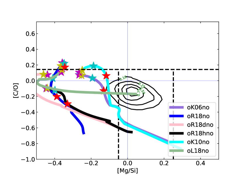
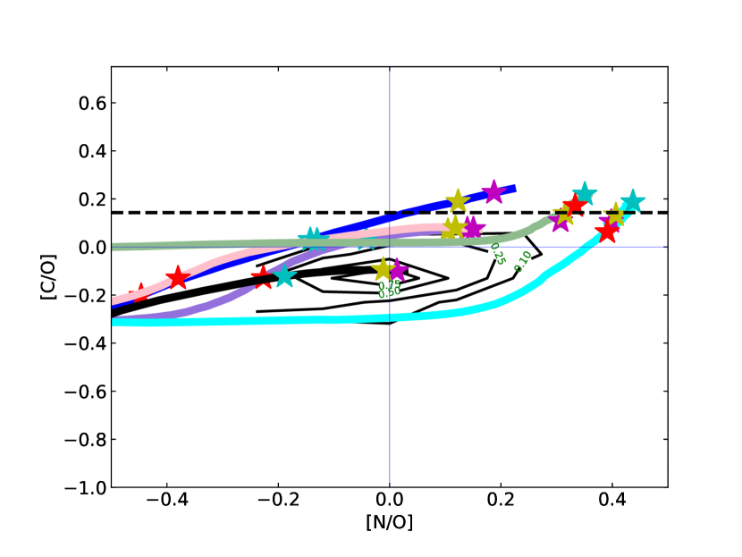
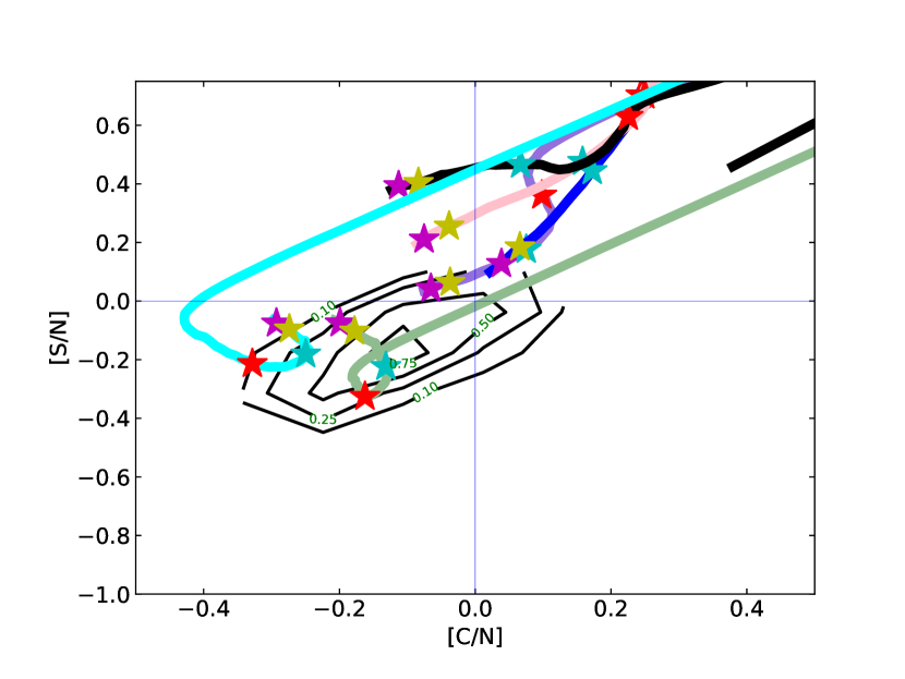
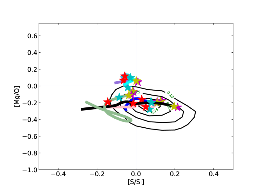
Figure 9: The same as in Figure 8, but with massive stars contributing to GCE up to M_up = 20M_⊙

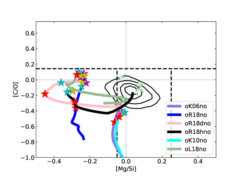
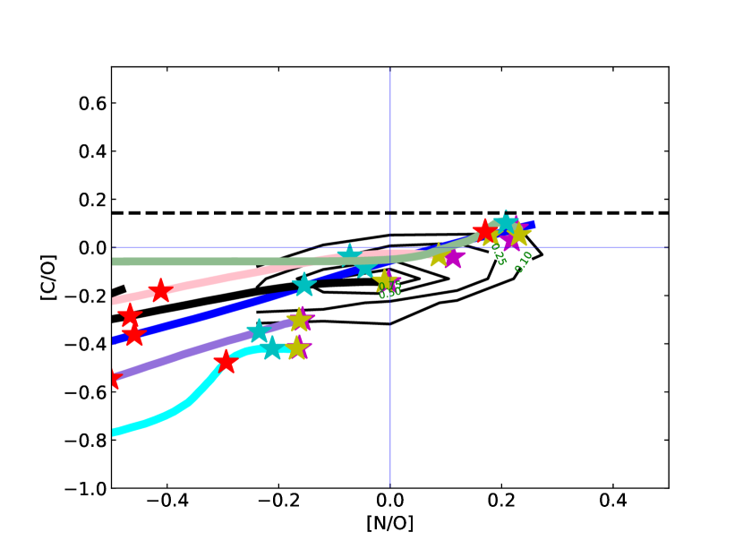
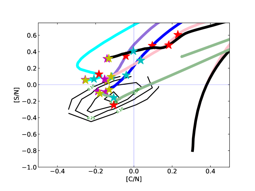
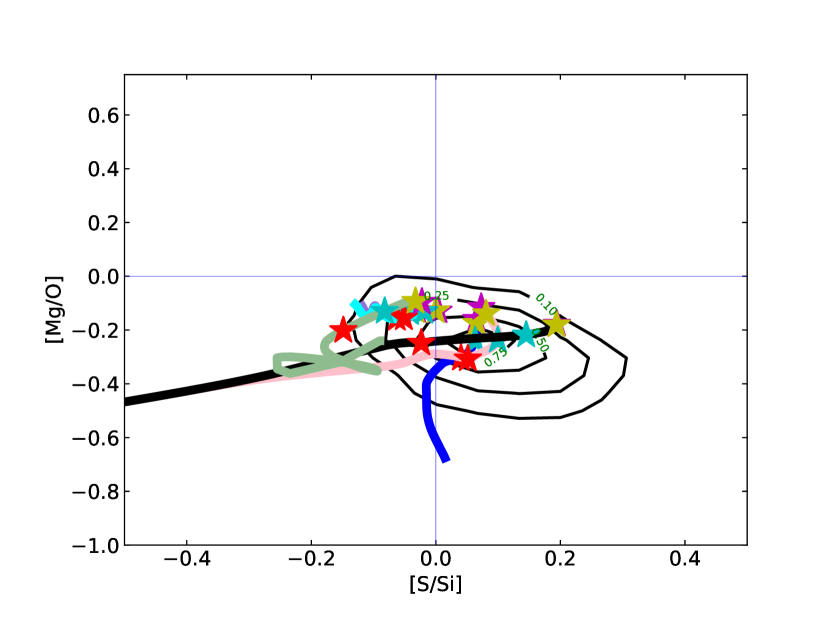
Figure 10: The same as in Figure 8, but with massive stars contributing to GCE up to M_up = 100M_⊙.

5.1 The effect of changing M_up in GCE simulations

The models shown in Figure 8 used as mass upper limit M_up = 40M_⊙ (Table 1). In Figure 9 and Figure 10 we have explored the impact of the M_up parameter space on the results, by considering M_up = 20 M_⊙ and M_up = 100 M_⊙, respectively. The upper-left panels of the two figures show that by increasing M_up, the predicted [Mg/Si] increases by up to 0.15 dex, but [C/O] decreases by up to 0.1 dex. For instance, with M_up= 100 M_⊙, the models oK06no and oK10no approach the solar [Mg/Si] ratio (the super-solar ratios observed are still not reproduced). Rather, the predicted [C/O] is about 0.3-0.4 dex lower than solar. On the other hand, with the extreme case M_up= 20 M_⊙, oK06no and oK10no predict a [Mg/Si]$\sim$-0.2 for the Sun, and for oL18no and all the oR18 models the same ratio is reduced down to about [Mg/Si]$\sim$-0.4. If we compare the upper-right panels, for models oK06no and oK10no the [N/O] typically decreases by 0.6 dex with increasing M_up, while there is mostly no effect in all the R18 models. This is because in our GCE models the total mass ejected for the higher masses is extrapolated from the list of available models, and the yields abundance pattern is kept identical to that of the highest mass model, which is the M=25M_⊙ progenitor for Ritter et al. and the M=40M_⊙ progenitor for Kobayashi et al. yields. The 25M_⊙ models by Ritter et al. are all weak explosions, leaving large remnants. Thus, stars between 25 and 100 M_⊙ only eject limited amounts of elements such as O and Mg. Notice that since L18 yields have large remnants for stars above 30 M_⊙, the M_up impact will be limited in these cases too. On the other hand, the yields by Kobayashi et al. (2006) are all made of successful CCSN explosions with low remnant masses, and increasing M_up of 20 to 100 M_⊙ makes a huge difference since more massive progenitors do contribute significantly to the chemical evolution.

The lower-left panel of Figure 9 shows that with M_up =20 M_⊙ the model oK10no can reach a sub-solar [S/N]$\sim$$-$0.2 dex, which would be consistent with the bulk of local stars, but with a [C/N]$\sim$-0.3 dex. The model oL18no can also reach a sub-solar [S/N]$\sim$$-$0.3 dex, with a [C/N]$\sim$-0.2 dex. All the other models exhibit a [S/N] range between solar and 2.5 times solar (oR18hno). With M_up = 100M_⊙ (Figure 10), the models closest to the observations are oR18no and oL18no with predicted [S/N] and [C/N] ratios in the range of $-$0.1 $-$ $-$0.2 dex, since the time of the formation of the Sun. Finally, if we compare the bottom right panels of Figure 9 and Figure 10, the only significant variation is a decrease of the [Mg/O] ratio of about 0.1 dex or less for all models with increasing M_up. Such a small variation is not surprising. Indeed, both O and Mg are mainly products of massive stars, they are made during the pre-SN stage and their pre-SN ratio is not significantly modified by the CCSN explosion (e.g., Thielemann et al., 1996; Pignatari et al., 2016).

In summary, from exploring the impact of the M_up parameter space we do not see a clear effect of using a value different from the default M_up =40 M_⊙. While a higher M_up slightly increases the [Mg/Si] ratio, it would still not cover the Sun and most of the stars, with the [C/O] ratio too low as compared to observations. The impact on the [N/O] and [S/N] ratios is model dependent. Therefore, in the following part of the section we will discuss only the models with M_up = 40M_⊙. Results for the same models but with different M_up are available in Appendix § A.

5.2 The impact of Faint Supernovae

To study the impact of faint CCSNe we focus our analysis to the two set of models using the yields K10 and R18 (Table 1). Results of other models are consistent with the sample of simulations considered here and are available in Appendix § A.

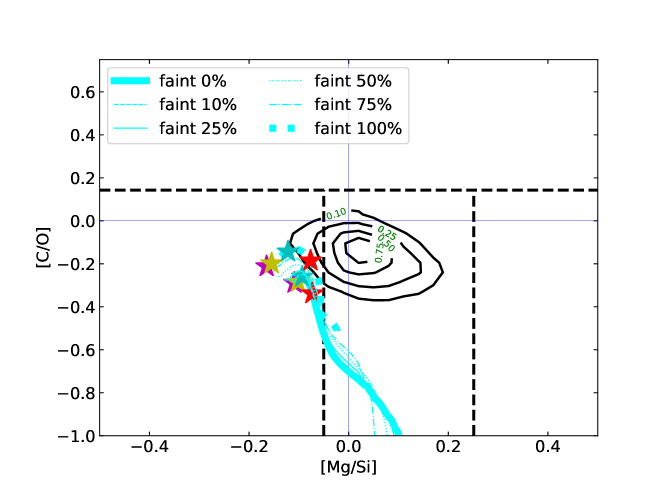
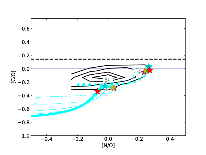
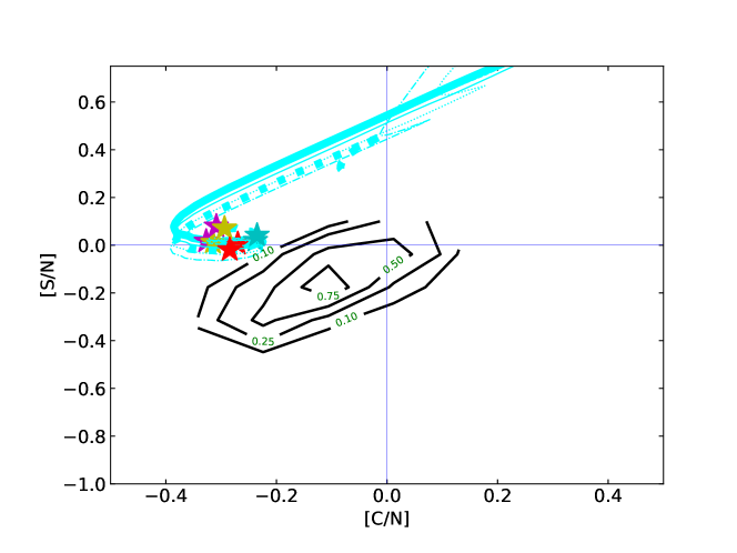
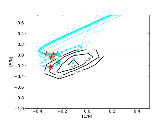
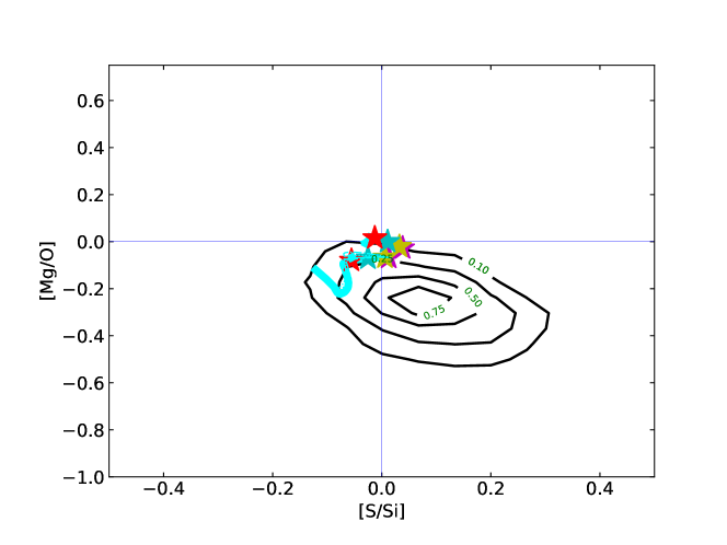
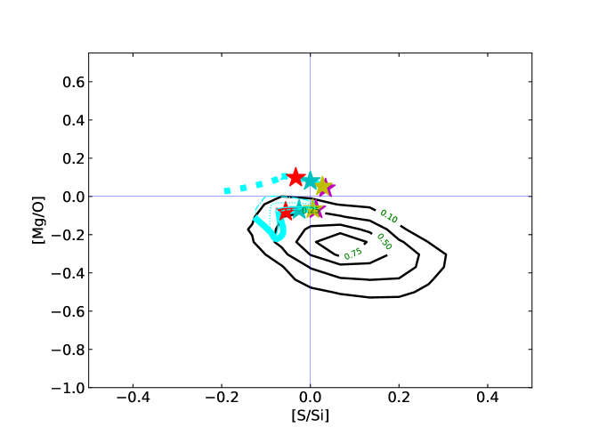
Figure 11: Selected elemental ratios normalized to the solar (L19$\_$3D by Lodders (2019), see Figure 5)

are plotted against each other for the GCE model set oK10, with CCSNe contribution up to M_up = 40 M_⊙ and using different fraction of faint CCSNe. As representatives of faint CCSNe, we use a 20M_⊙ model and a 25M_⊙ model (left and right panels, respectively, see Table 1). For comparison, observations from the solar neighbourhood stars are reported as in the previous figures.

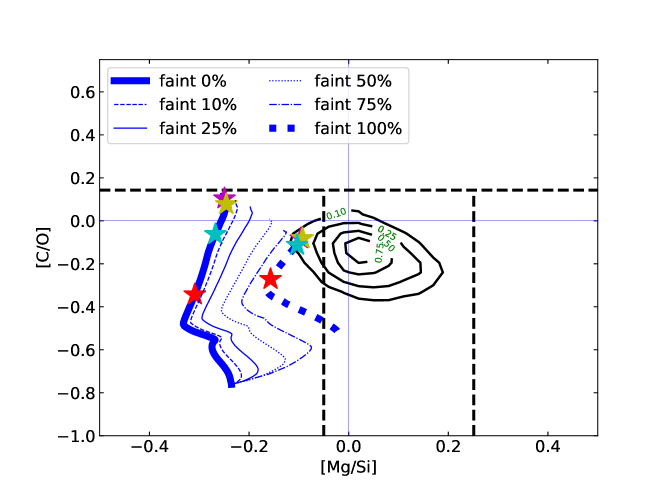
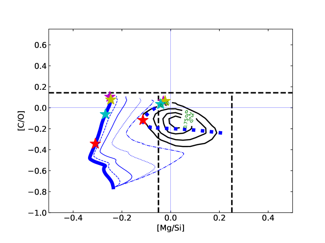
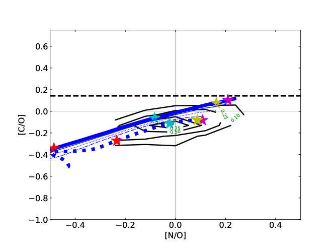
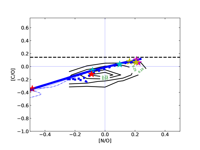
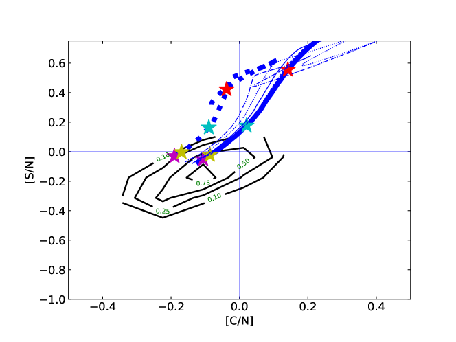
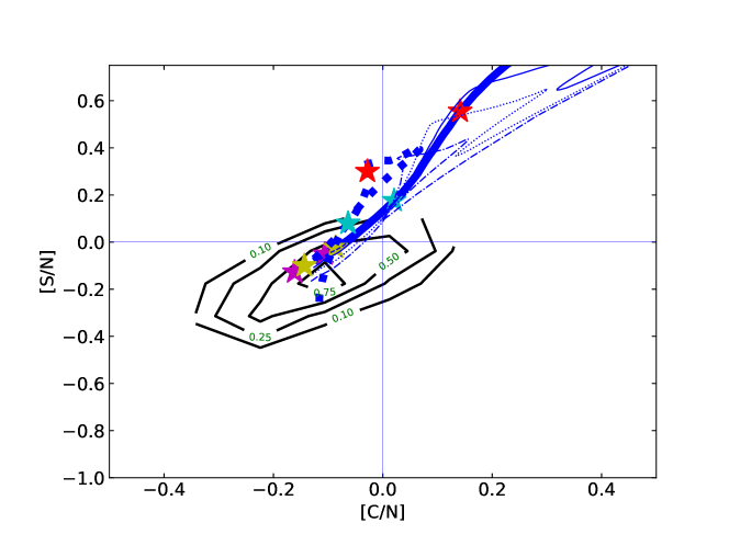
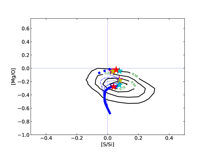
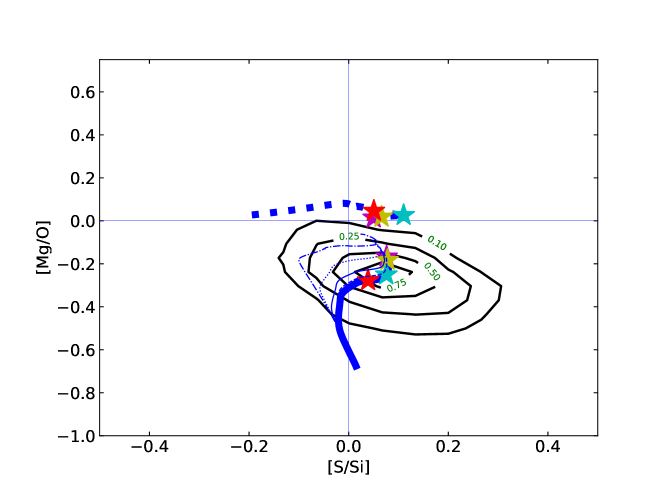
Figure 12: Same as in Figure 11, but for the GCE model set oR18.

Figure 11 reports the impact of faint CCSNe for the oK10 models. The full parameter space is considered, with the frequency of faint CCSNe from 0% (which would correspond to the oK10no model shown in Figure 8) to 100% (models oK10<faintSN$\_$model>f1p00). As representative of faint CCSNe models, we used the 20 M_⊙ (m20) and 25 M_⊙ (m25) CCSN models by Ritter et al. (2018b) shown in Figure 2 (models oK10m20<faintSN$\_$weight> and oK10m25<faintSN$\_$weight>, respectively). As seen in Section § 2, the m20 model still ejects some material carrying the signature of O-burning, while there is no Fe-rich Si-burning ejecta. The m25 model does not eject products of either Si-burning or O-burning. Note that considering present uncertainties in CCSN explosion and the wide zoo of CCSN remnants presently observed, we may expect the real fraction of faint CCSNe to be somewhere in between the two extreme cases, oK10no and oK10<faintSN$\_$model>f1p00. In the left panels of Figure 11, no substantial effect is observed from considering faint CCSNe. The first reason is that CNO elements are not substantially affected by the CCSN explosion as they are mostly produced during stellar evolution before core collapse. Therefore, their relative abundances do not change significantly in faint CCSNe, as compared to standard CCSNe. The second reason is that although Si and S are O-burning products, the m20 faint CCSNe model used in these tests still eject some Si-rich and S-rich material, without affecting the [S/N] and the [S/Si] ratios much.

The impact of faint CCSNe becomes more relevant in the GCE models where m25 is used. In the upper-right panel of Figure 11, [C/O] and [Mg/Si] increase by about 0.2 dex and 0.1 dex respectively, when comparing oK10m25f0p50 to oK10no. Models with higher faint CCSNe frequency oK10m25f0p75, oK10m25f0p90 and oK10m25f1p00 have even larger increases, up to solar ratios. We would, however, consider these last models of the parametric study as less realistic. The reason for the impact on [C/O] is that a significant part of the former O-rich C shell is not ejected by m25 (Figure 2). Therefore, the overall galactic enrichment is driven to higher C/O-ratios. The impact on [Mg/Si] is instead smaller, since, as with O, Mg-rich material is not fully ejected by this model. A faint CCSN model with a lower masscut allows for more O and Mg ejection and still no O-burning products like Si. This is still realistic to consider within the uncertainties (e.g., Fryer et al., 2018) and would, in principle, achieve larger [Mg/Si]. The impact on the [C/O] would be small. In the second from top right panel of Figure 11, [N/O] increases with increasing the faint CCSNe frequency, up to +0.35. The effect on the [N/O] ratio is the same as discussed for the [C/O] ratio, where N is mostly made in the most external layers of CCSNe. The model oK10m25f0p50 shows a reduction of the [S/N] ratio down to $-$0.15, providing a possible explanation of the observation range. As we mentioned in the previous section, however, the nucleosynthesis of N in CCSNe may be affected by physics not considered in this work, like stellar rotation or H-ingestion events, which would both increase the N yields as compared to S. Finally, also in this case there are only minor effects on the [Mg/O] and [S/Si] ratios.

Figure 12 presents the equivalent oR18 models. Qualitatively, there are similar effects using the m20 and m25 faint CCSNe as debated above for the oK10 models, with overall a more significant impact in the oR18m25<faintSN$\_$weight> models. The top panels confirm the increasing trend of [Mg/Si] with the faint SN frequency, with a ratio higher than about 0.1 dex in the oR18m20f0p50 and oR18m25f0p50 with respect to oR18no. Instead, the [C/O] increase is more limited, as compared to the oK10 models, and more dependent on the evolution time of the model. The evolution of the [N/O] ratio in the oR18 models is also different compared to the effect seen in the oK10 models. While the final abundances vary by less than 0.1 dex between oR18m20no and oR18m20f1p00 and are mostly unaffected when using the m25 faint CCSN model, the ratio starts to increase at much earlier times, with the [N/O] ratio higher up to 0.4 dex. The impact on the final [S/N] in the oR18 models including faint CCSNe is less than 0.1 dex, while it was more significant in oK10 models using an m25 faint CCSN. Finally, like for the oK10 models, there is no effect on the [S/Si] ratio. There is instead an increase of the [Mg/O] ratio, by less than 0.1 dex, between the oR18m20f0p50 and oR18m25f0p50 with respect to oR18no, with an increase up to 0.2 dex reaching the solar ratio for oR18m20f1p00 and oR18m25f1p00.

6 Summary and Conclusions

We presented 198 new GCE simulations of the solar neighbourhood, with the main goal to study the production and evolution of the important planet-building nuclides C, N, O, Mg, Si, and S, in comparison to stellar observations. We chose these elements because results from simulations of planet formation and evolution depend on their initial abundances (e.g., Frank et al., 2014). One of the fundamental purposes of this work is also to provide an accessible (but comprehensive) picture about the challenges and the uncertainties in stellar simulations, observations and GCE, and at the same time we also want to make clear what are the needs of planet-formation and evolution studies from observations and from GCE, in the light of present and future opportunities to unfold thanks to the new generation of observation facilities. The new data coming from TESS (Ricker et al., 2015) and from JWST (Beichman et al., 2014), as well as from future facilities like ARIEL (Tinetti et al., 2018; Turrini et al., 2018, 2021), will complement those being provided by ongoing ground-based efforts (e.g. Giacobbe et al., 2021; Carleo et al., 2022; Guilluy et al., 2022) and we can anticipate a greatly enhanced window with which to study these processes in more detail. In this context, GCE models provide the initial composition of stars and of their proto-planetary disks where planets are formed at different times and locations in the Galaxy for all the elements. Based on theoretical simulations and observations, we also expect that planet-formation processes will drastically affect some of the planet abundances measured today with respect to the pristine abundances of the proto-planetary disk, while others will only be marginally affected. The results of GCE models provide therefore a crucial additional benchmark for simulations of planet formation, in particular when elemental abundances from the stellar host are uncertain or not available.

The GCE simulation framework presented here is made of five sets of models, where the impacts of stellar yields, of the stellar mass upper limit contributing to the chemical evolution (M_up) and of faint CCSNe were explored. With our models, classical stellar sources used to reproduce the evolution of the elements C, N, O, Mg, Si and S are not able to fully reproduce the solar abundances, and/or the observed range in the solar neighbourhood, in particular for the [C/O] and [Mg/Si] diagram. In our analysis, we did not apply any corrections to force the results from GCE simulations to match the solar abundances. The chemical enrichment history of these elements in the Milky Way is complicated, since all the contributions from CCSNe, SNIa and AGB stars must be taken into account, along with their different timescales (e.g., Mollá et al., 2015; Mishenina et al., 2017; Prantzos et al., 2018; Kobayashi et al., 2020b).

We did not find a specific set of yields that is able to solve all the ratios considered in our analysis within the correct GCE evolution timescale. We also show that the impact of M_up is in general limited for these elements considered, and it is model dependent.

By considering realistic frequencies of faint CCSNe, we obtain instead variations of elemental ratios in the order of 0.1-0.2 dex. In particular, we find that the increase of [C/O] and [Mg/Si] with increasing faint CCSN frequency may help to better reproduce the abundances observed in stars in the solar neighbourhood. The potential reduction of [S/N] in the order of 0.2 dex can also help match the range of observations, with its impact depending on the set of CCSN yields adopted.

The reduction of the observational uncertainties for the elements considered will be a crucial step towards solving present discrepancies between GCE simulations and observations. The more limited abundance dispersion in the stellar sample by Bedell et al. (2018) compared to other analogous works requires independent verification. Ramírez et al. (2014) discussed the star-to-star scatter for different elements, showing that while several elements (including O and Si discussed in this paper) present a variation compatible with the measurement errors, other elements not discussed here (e.g., Na, Al, V, Y, and Ba) may have larger discrepancies. From a similar analysis Adibekyan et al. (2015b) instead found that the star-to-star scatter may simply increase with the decrease of the number of spectral lines used in the derivation of the abundances. This would indicate that a good fraction of the observed scatter is not astrophysical. In more general terms, the comparison between data from different observational surveys obtained using different spectral lines and stellar parameters should be undertaken with caution. New comprehensive atomic physics investigations of transition probabilities for relevant spectral lines are further needed in order to improve the present results.

We have highlighted how a different definition of solar references provide a major additional source of uncertainty. We have shown that spectroscopic observations vary significantly between different works once absolute abundances are compared instead of those normalised to solar. Planet-formation simulations, however, use absolute pristine stellar abundances as a starting point, and therefore they are directly affected (Spaargaren et al., 2023). Alongside C, N, O, Mg, Si, and S discussed in this work, elements of interest for planet-formation studies include lithophile elements such as Cl, Cr, K, Na, V, P, Ti, Al and Ca the abundances of which can potentially be better constrained by future facilities such as ARIEL (Tinetti et al., 2018; Turrini et al., 2018). As discussed by Turrini et al. (2021) and Turrini et al. (2022) each of these elements, being more refractory than O, can be used in place of S to study the planet-formation history together with C, N and O. As the accuracy of atmospheric retrieval methods for exoplanetary observations is currently capped to about 10-20% (see Barstow et al., 2020; Turrini et al., 2022, for discussion), the characterisation of stellar abundances with the precision of 0.1 dex would provide a solid base for the next generation of planet-formation studies to compare with atmospheric data. Note that Fe is another element essential for mineralogy and planet formation, but it is not included in the analysis presented here. Undeniably, CCSNe yields for Fe are quite uncertain (e.g., Pignatari et al., 2016; Sukhbold et al., 2016; Curtis et al., 2019), and stellar-yields uncertainties are then propagated to GCE, where additional uncertainties include for instance assigning the correct populations of SNIa contributing to GCE (e.g., Lach et al., 2020; Gronow et al., 2021b). We therefore report the study of the GCE of Fe and of the Fe-group elements (for a consistent analysis they cannot be treated separately) in the Milky Way disk as a separate work (Trueman et al., submitted).

Once the uncertainties in spectroscopic observations and in the solar composition are sufficiently reduced, GCE simulations hold the potential to generate a robust fit to the compositional catalogue of stars in the solar neighbourhood. Notwithstanding, more powerful constraints need to be derived on the role of faint CCSNe required to cover the full range of observations.

Data Availability

The data generated for this article will be shared on reasonable request to the corresponding author.

Appendix A Complete list of figures for GCE simulations

In this section the full list of figures exploring the impact of both M_up and faint supernovae parameter spaces in GCE simulations are provided.

As in Figure 11 for the oK10 set, the results from oK06 models with M_up=40M_⊙ are shown using faint supernova models m20 and m25 in Figure 13. The same is done for M_up=20M_⊙ and M_up=100M_⊙ in Figures 14 and 15, respectively.

For oK10, the results using M_up=20M_⊙ and 100M_⊙ for different faint supernovae are given in Figures 16 and 17. The same results for M_up=40M_⊙ are discussed in section § 5 (Figure 11).

For the oR18 set, the results using M_up=20M_⊙ and 100M_⊙ for different faint supernovae are given in Figures 18 and 19. The same results for M_up=40M_⊙ are discussed in section § 5 (Figure 12).

For models oR18d, the results using M_up=40M_⊙, 20M_⊙ and 100M_⊙ for different faint supernovae are given in Figures 20, 21 and 22, respectively. For models oR18h the results results using M_up=40M_⊙, 20M_⊙ and 100M_⊙ for different faint supernovae are given in Figures 23, 24 and 25, respectively. Finally, the same is reported for models oL18 in Figures 26, 27 and 28, respectively.

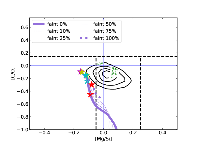
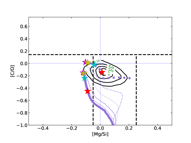
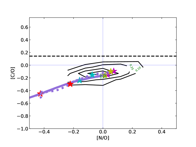
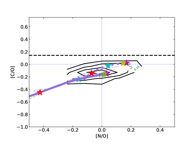
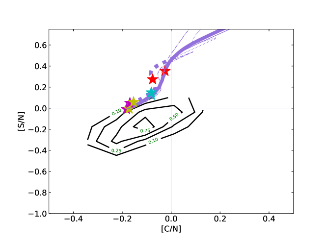
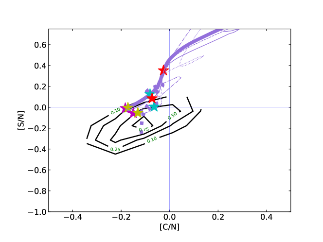
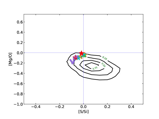
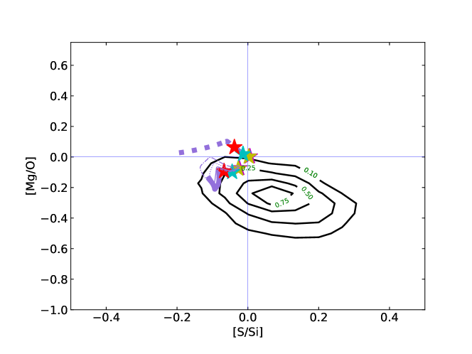
Figure 13: Same as in Figure 11, but for the GCE model set oK06.

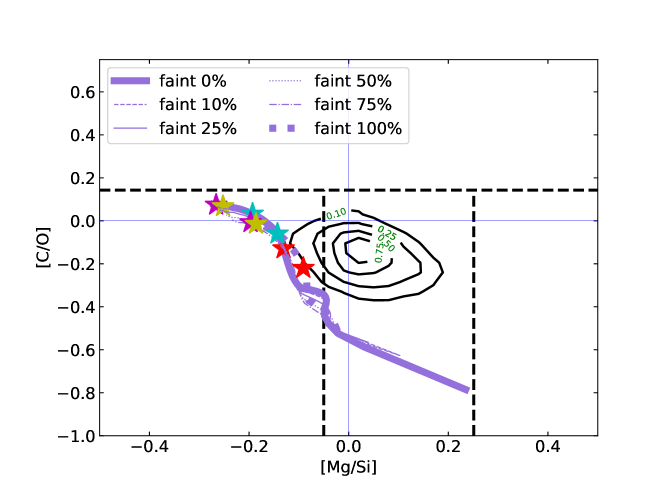
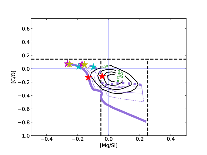
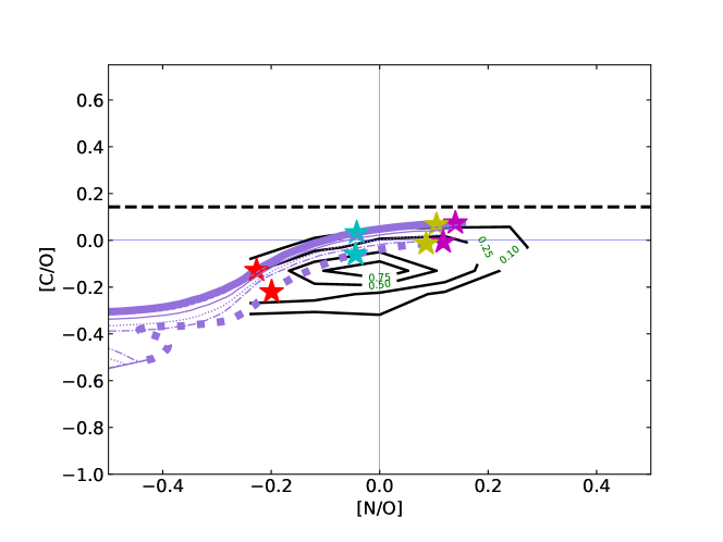
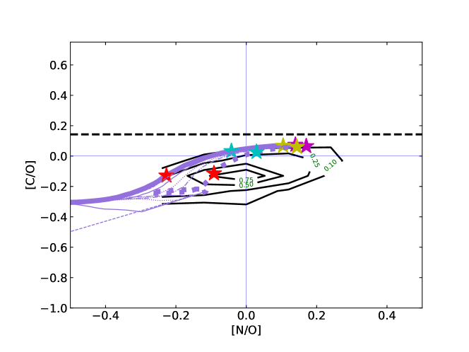
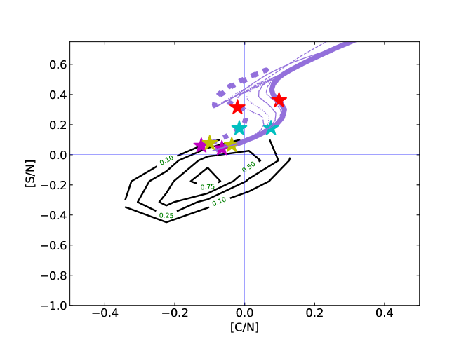
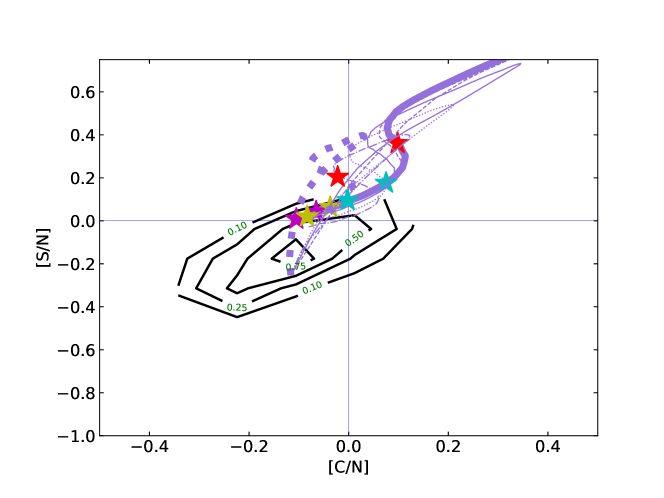
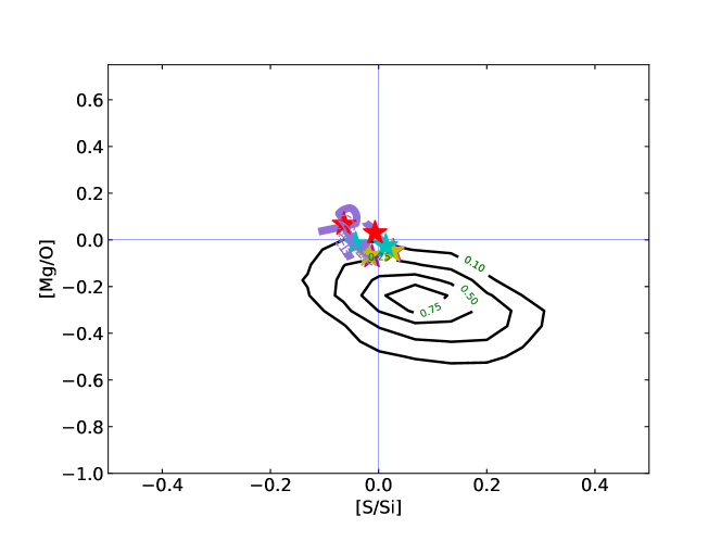
Figure 14: As in figure 13, but models are shown with CCSN supernovae contribution up to M_up = 20 M_⊙.

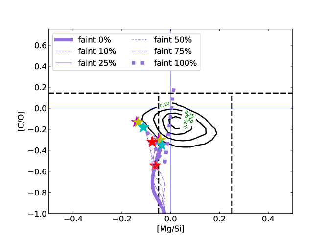
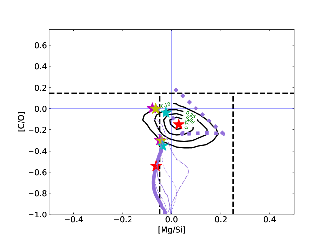
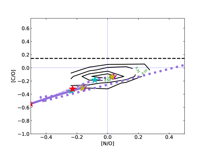
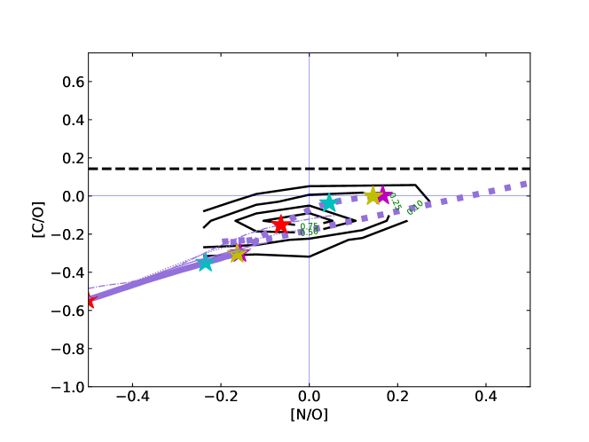
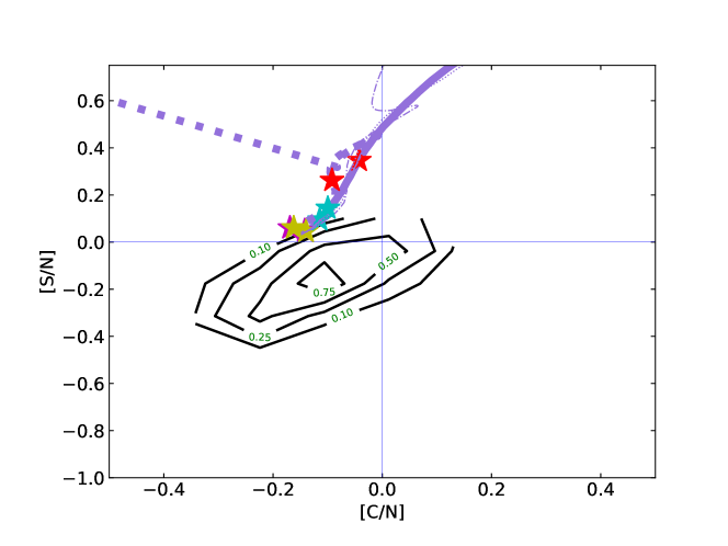
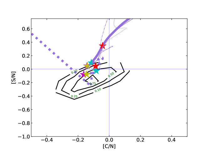
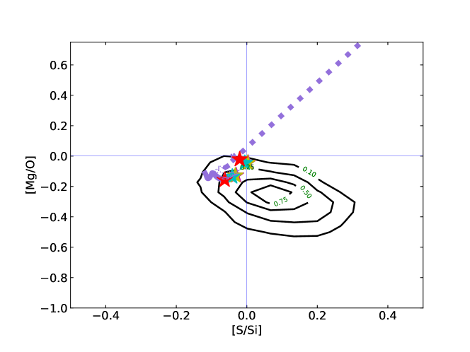
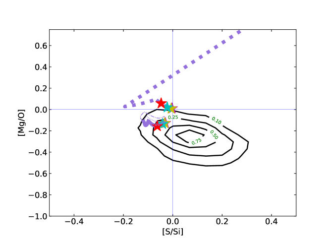
Figure 15: As in figure 13, but models are shown with CCSN supernovae contribution up to M_up = 100 M_⊙.

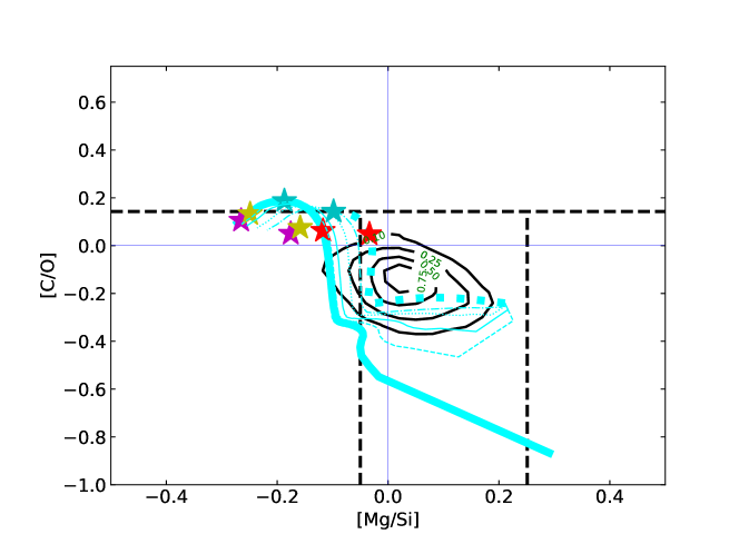
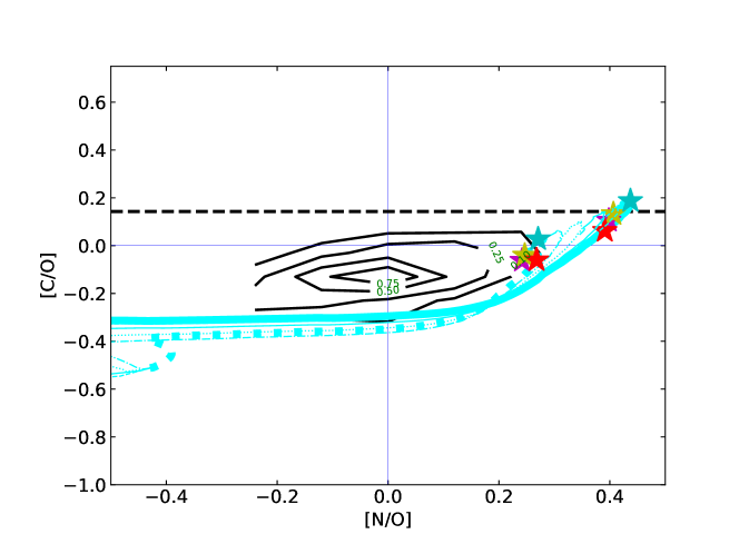
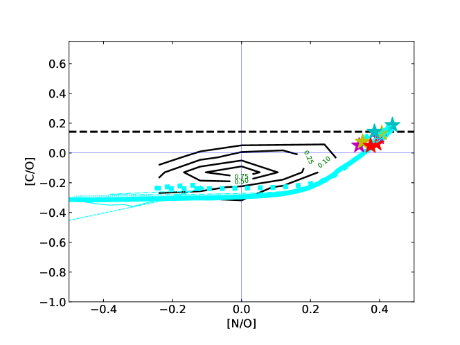
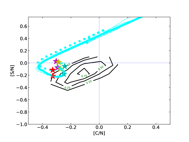
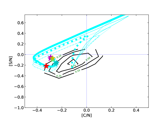
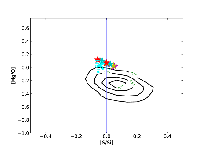
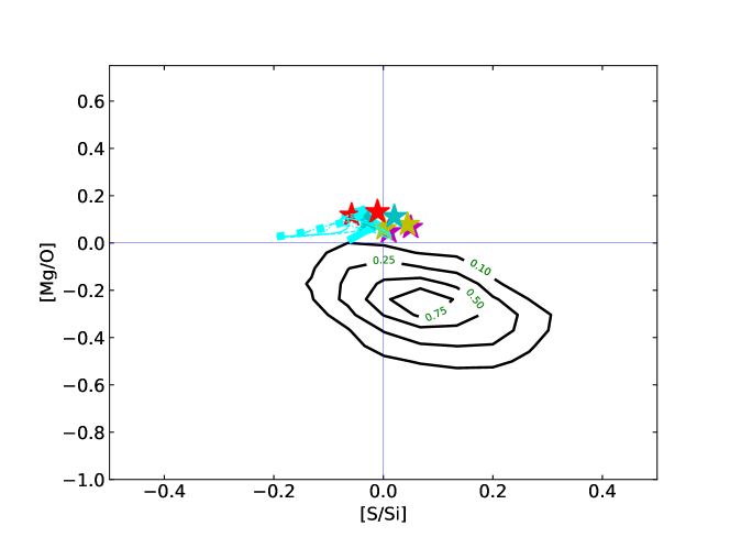
Figure 16: As in figure 11 for the oK10 model set, but models are shown with CCSN supernovae contribution up to M_up = 20 M_⊙.

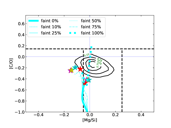
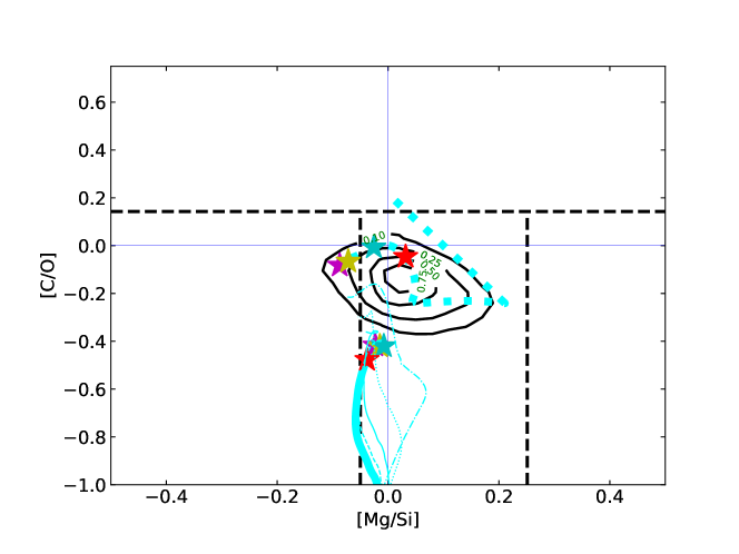
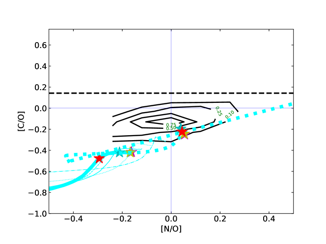
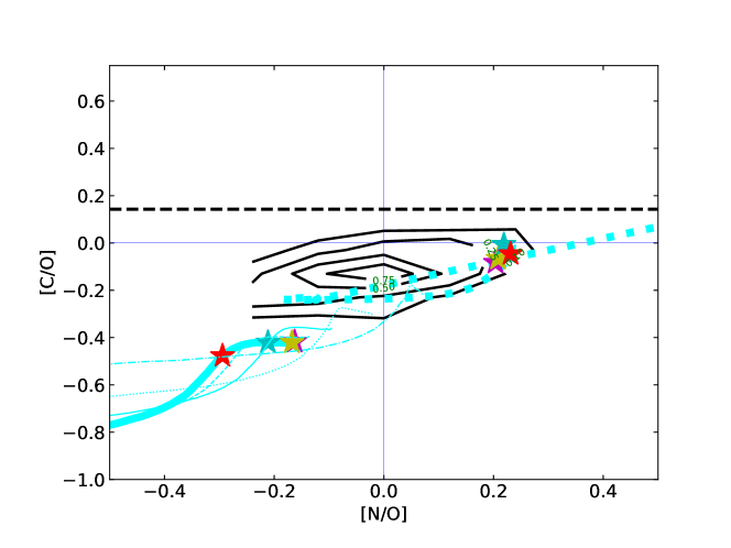
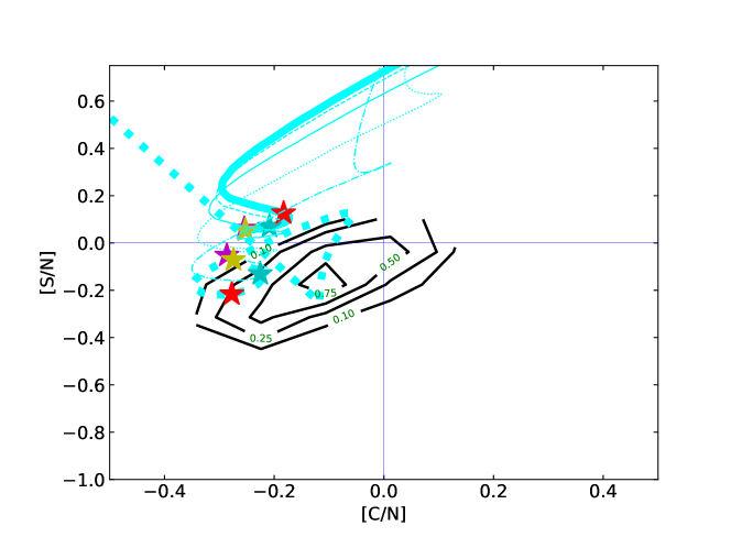
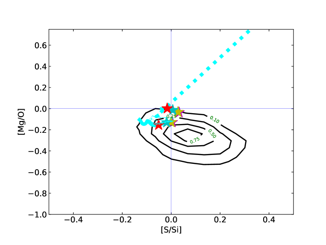
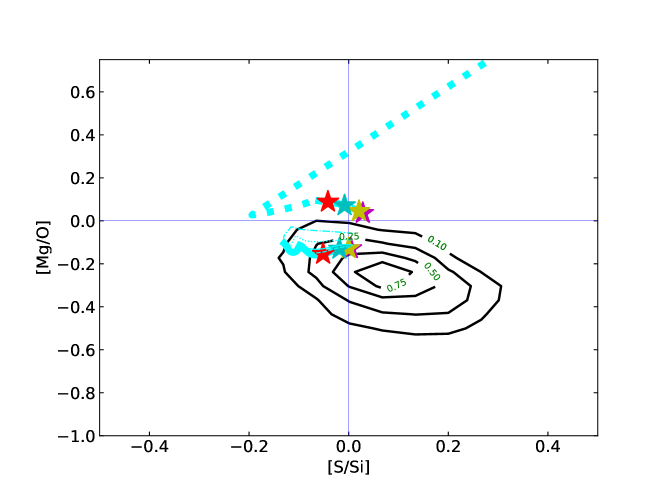
Figure 17: As in figure 11 for the oK10 model set, but models are shown with CCSN supernovae contribution up to M_up = 100 M_⊙.

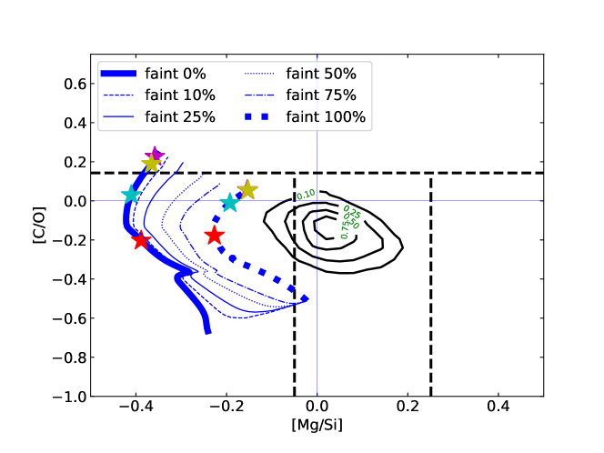
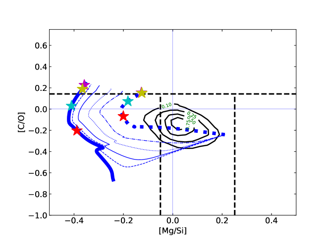
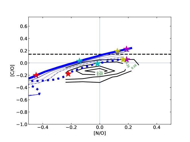
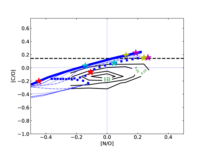
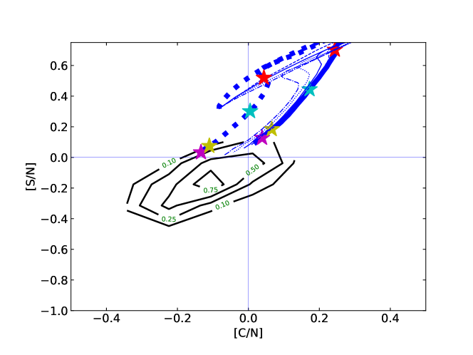
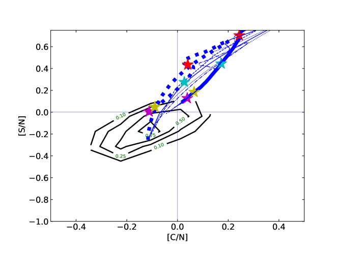
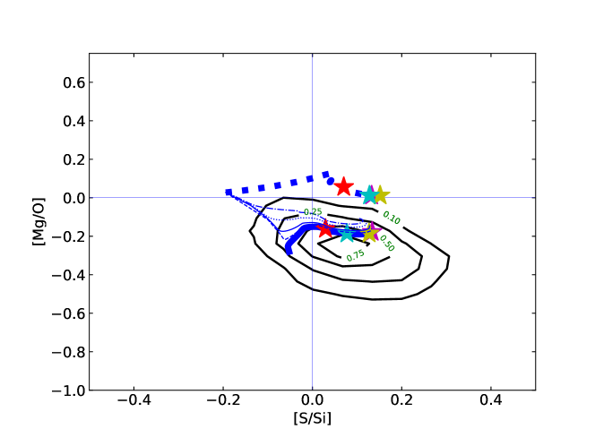
Figure 18: As in figure 12 for the oR18 set, but models are shown with CCSN supernovae contribution up to M_up = 20 M_⊙.

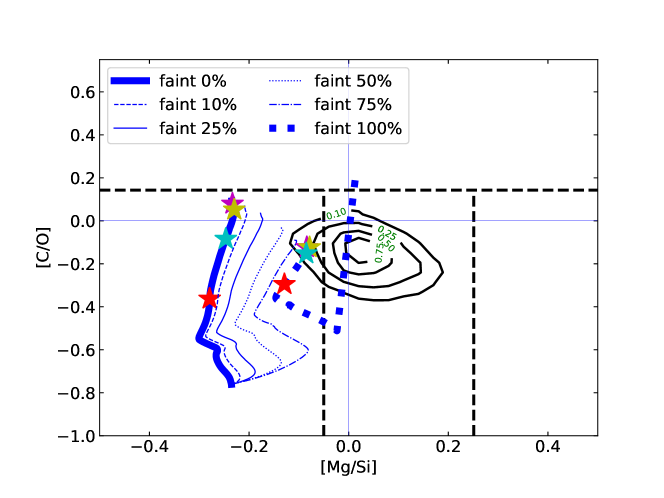
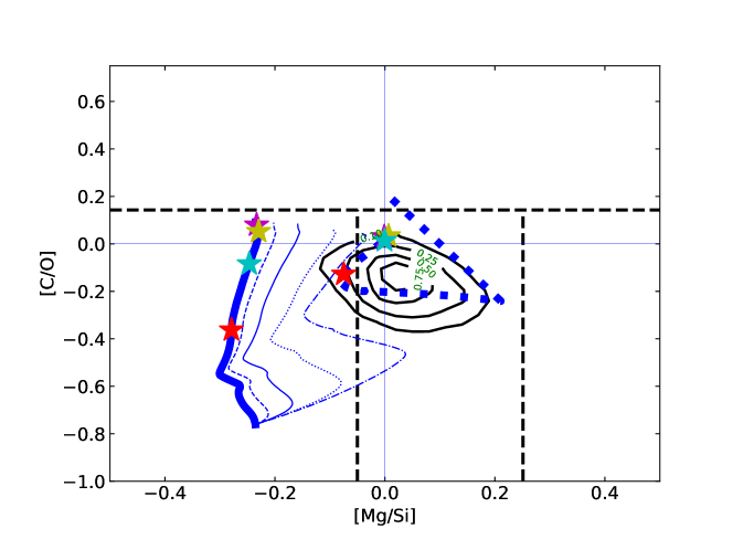
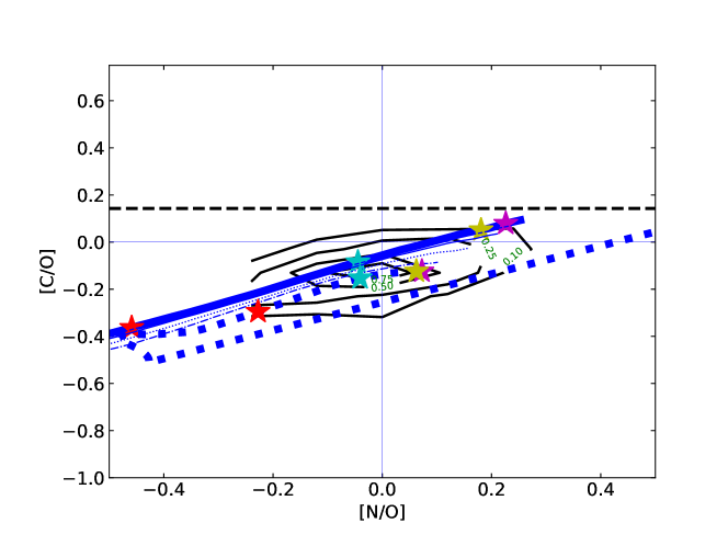
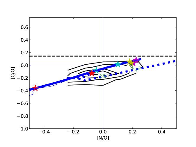
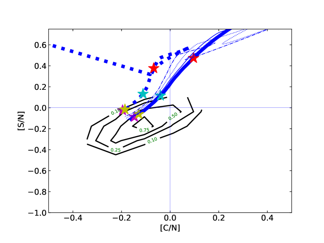
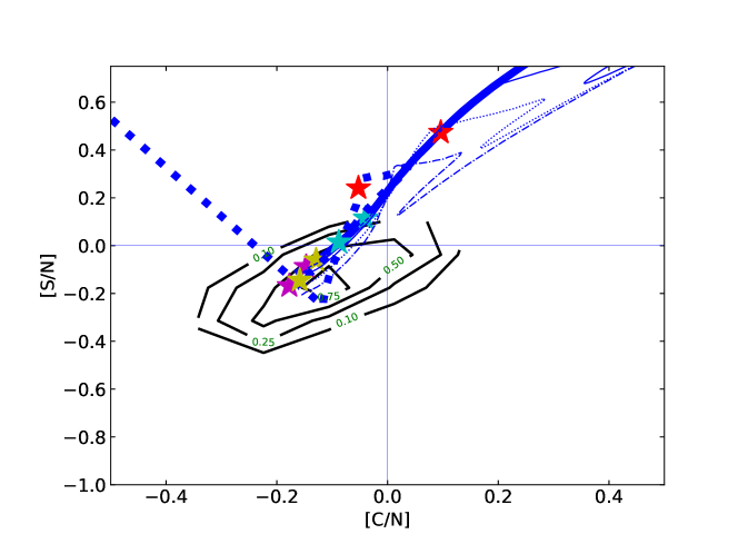
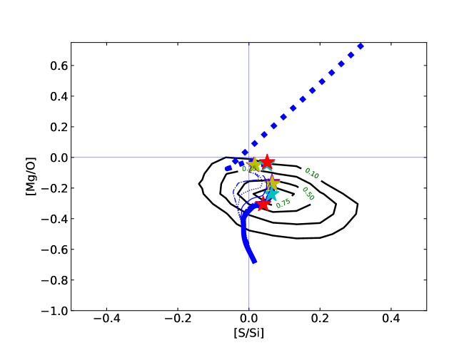
Figure 19: As in figure 12 for the oR18 set, but models are shown with CCSN supernovae contribution up to M_up = 100 M_⊙.

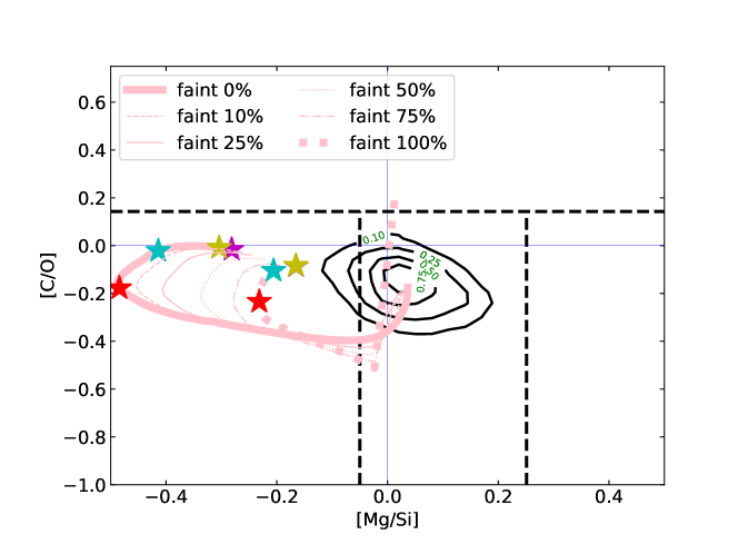
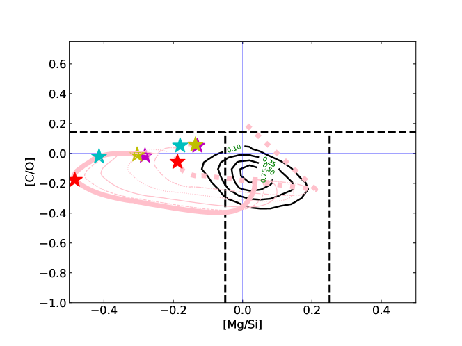
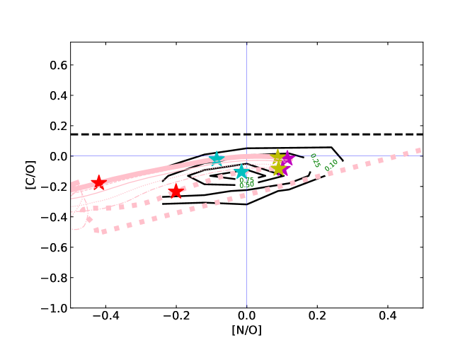
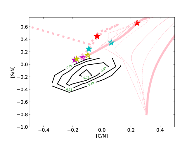
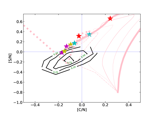
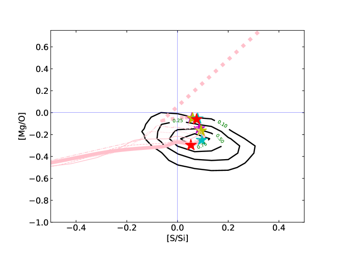
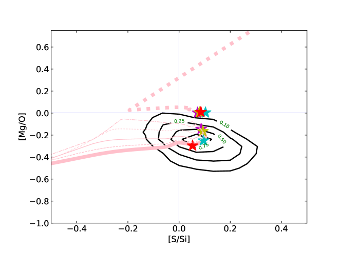
Figure 20: Same as in Figure 11, but for the GCE model set oR18d.

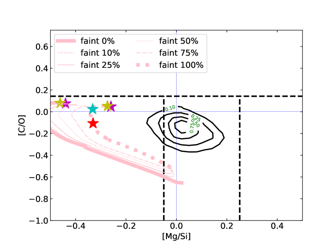
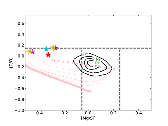
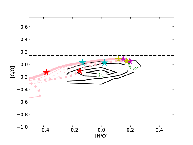
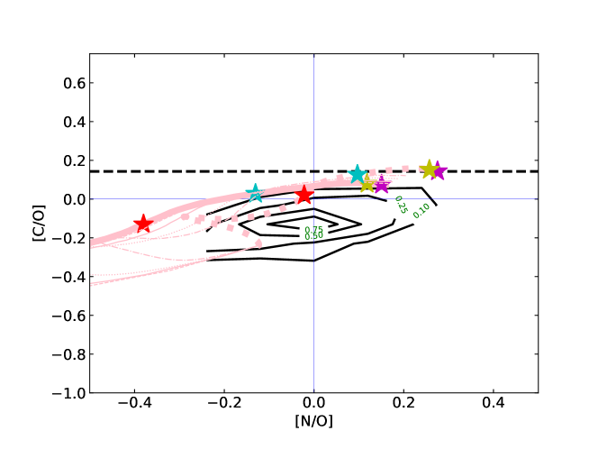
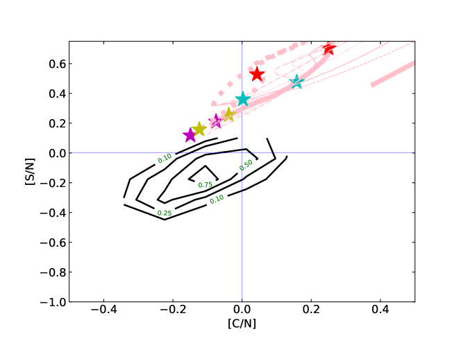
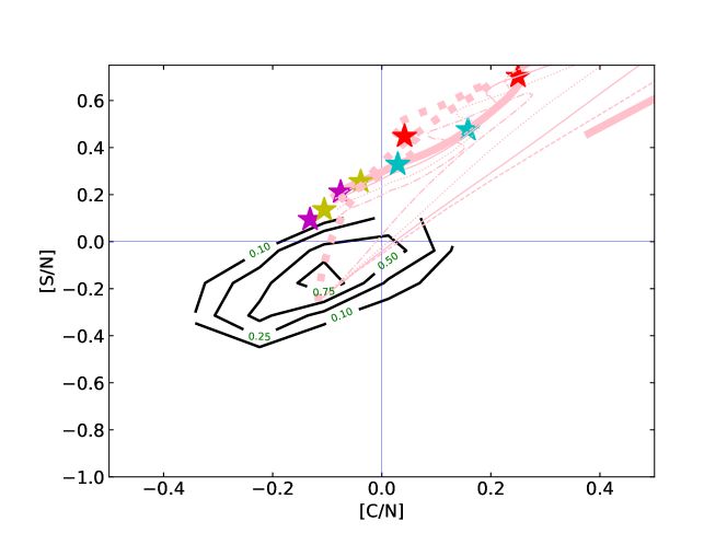
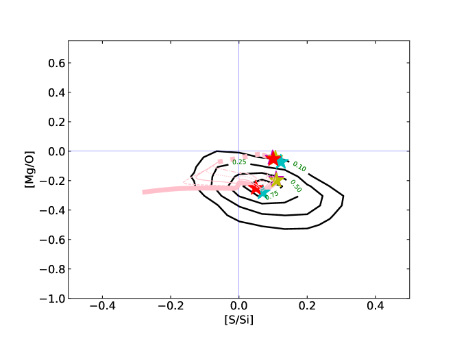
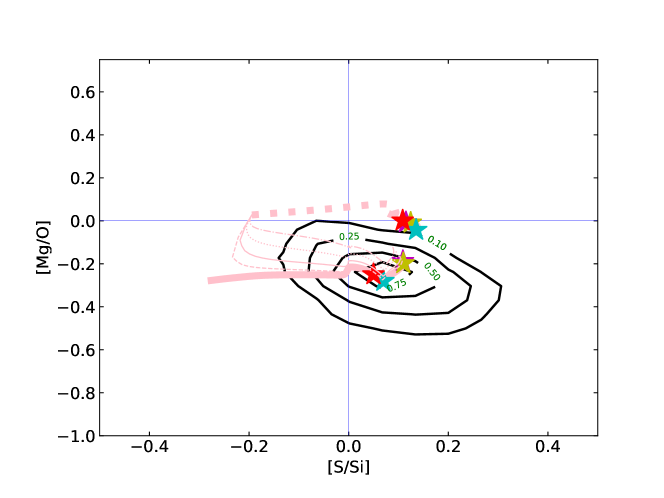
Figure 21: As in figure 20, but models are shown with CCSN supernovae contribution up to M_up = 20 M_⊙.

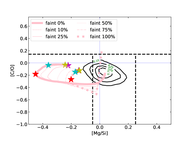
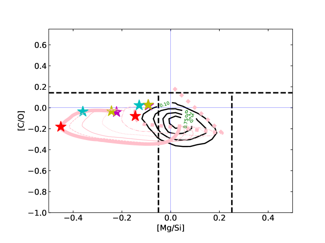
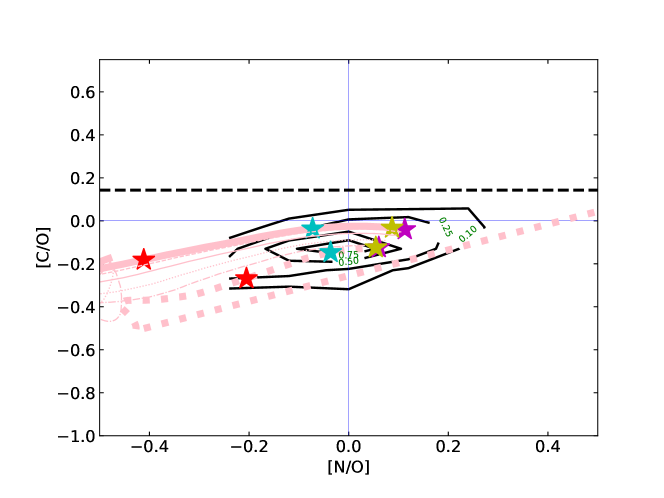
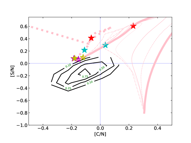
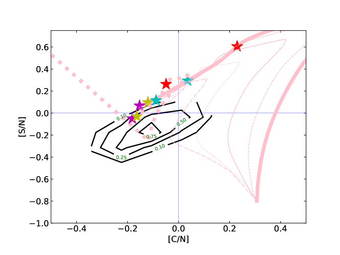
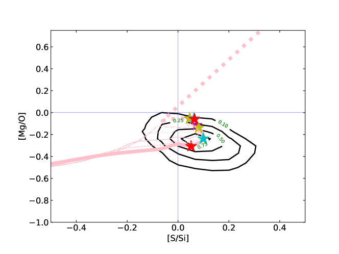
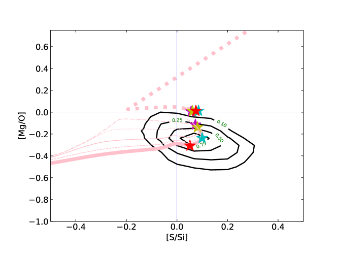
Figure 22: As in figure 20, but models are shown with CCSN supernovae contribution up to M_up = 100 M_⊙.

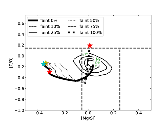
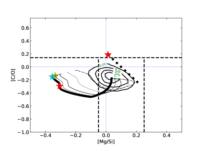
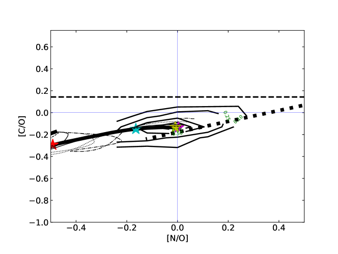
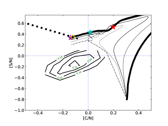
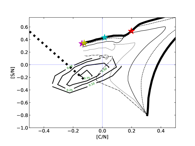
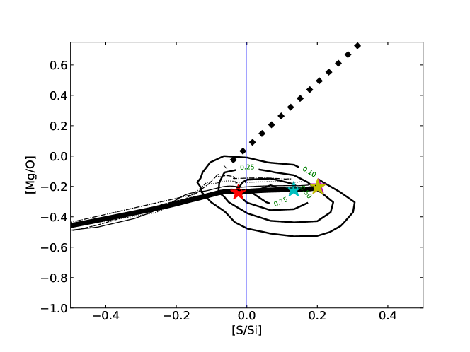
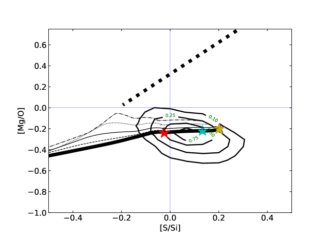
Figure 23: Same as in Figure 11, but for the GCE model set oR18h.

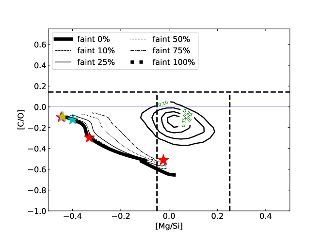
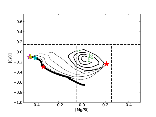
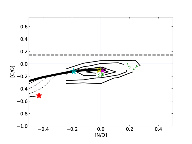
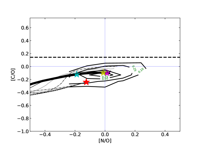
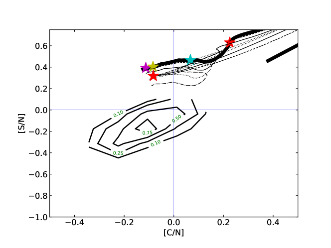
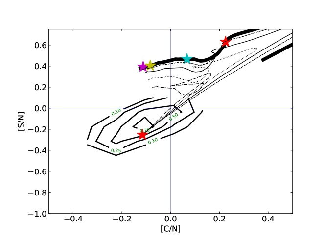
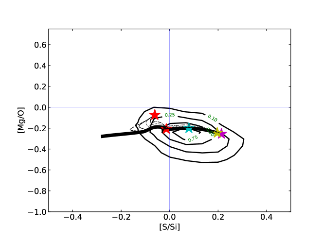
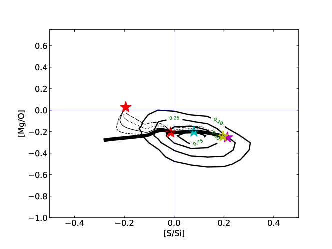
Figure 24: As in figure 23, but models are shown with CCSN supernovae contribution up to M=20M_⊙.

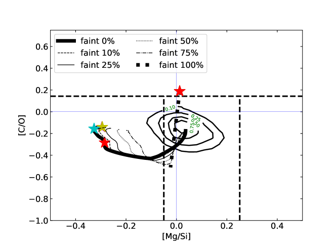
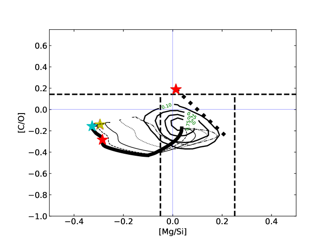
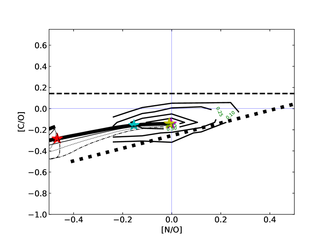
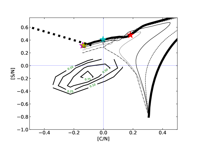
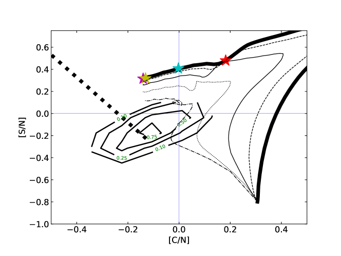
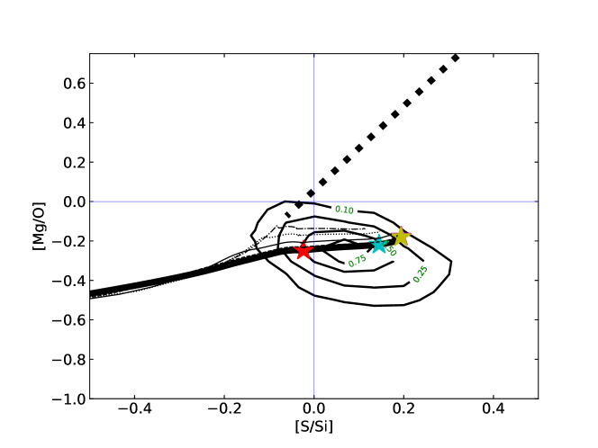
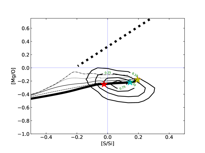
Figure 25: As in figure 23, but models are shown with CCSN supernovae contribution up to M_up = 100 M_⊙.

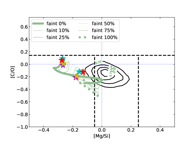
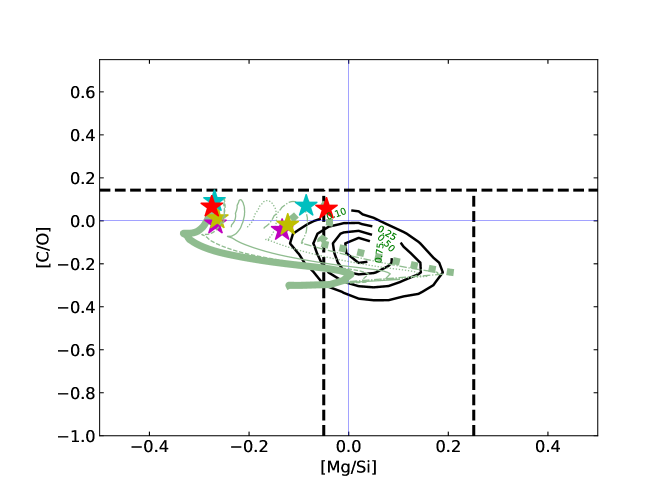
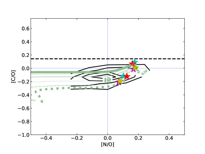
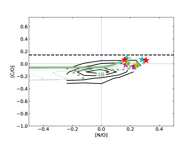
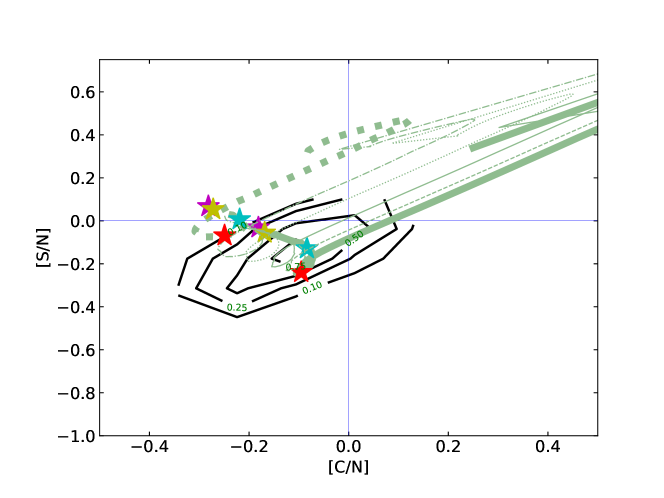
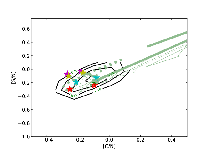
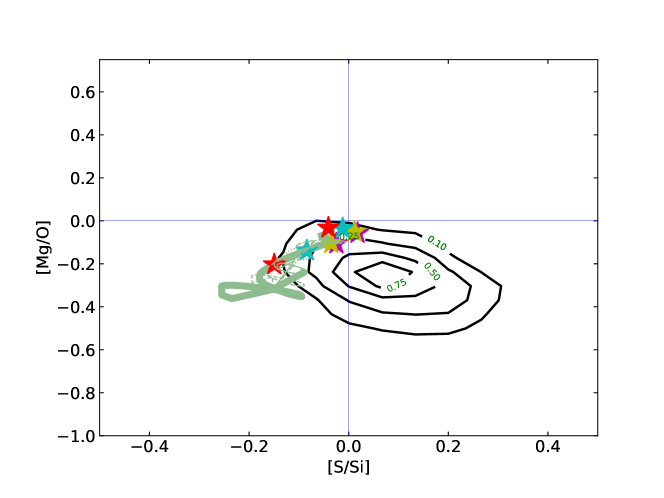
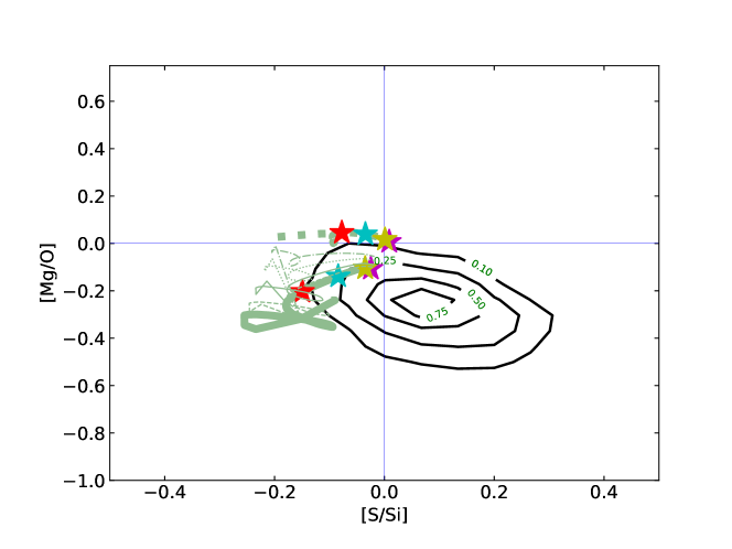
Figure 26: Same as in Figure 11, but for the GCE model set oL18.

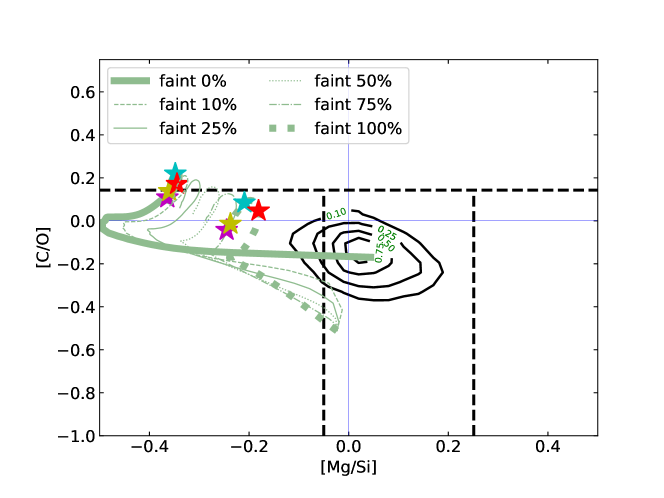
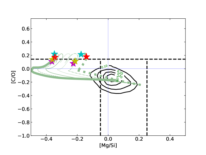
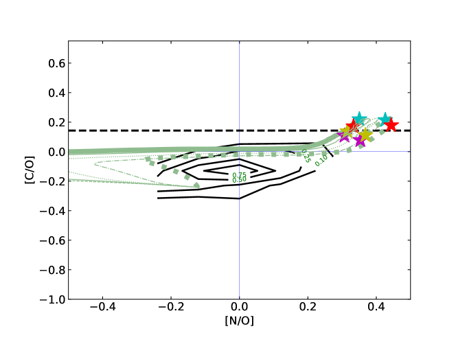
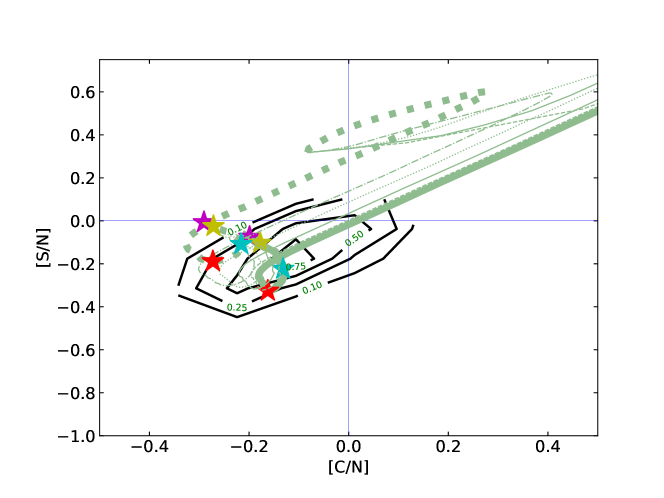
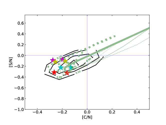
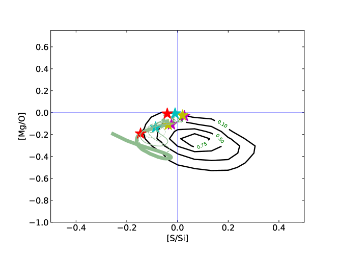
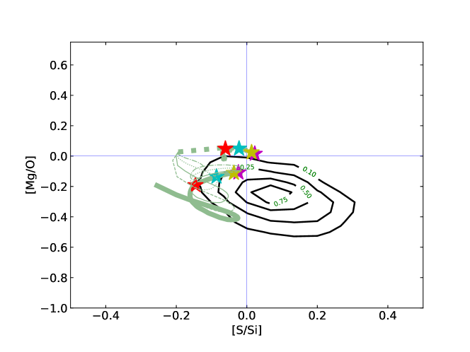
Figure 27: As in figure 26, but models are shown with CCSN supernovae contribution up to M_up = 20 M_⊙.

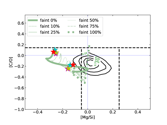
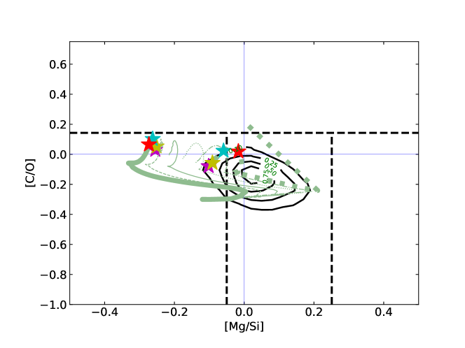
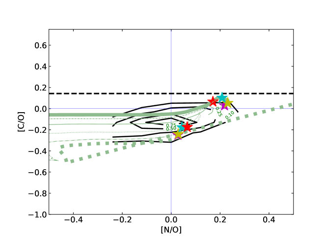
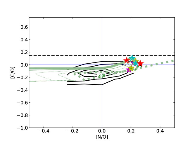
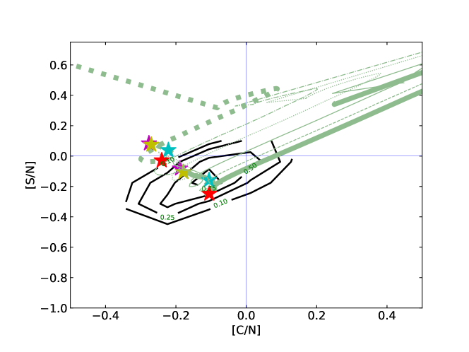
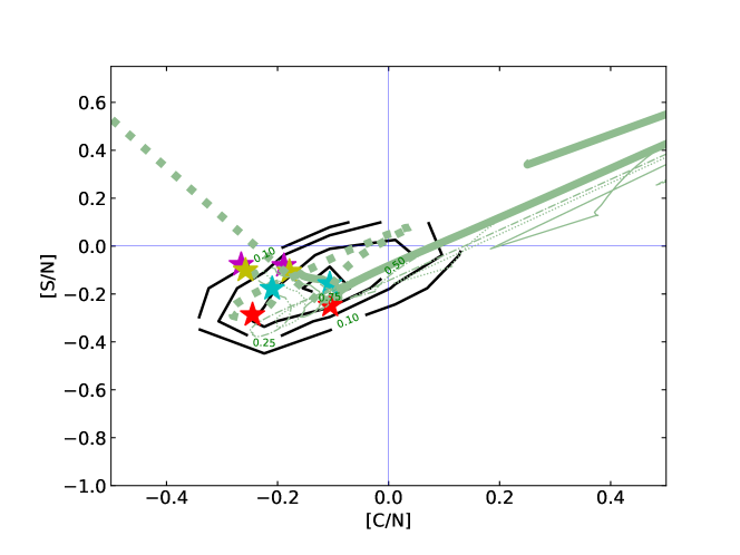
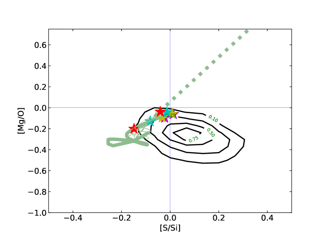
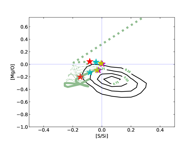
Figure 28: As in figure 26, but models are shown with CCSN supernovae contribution up to M_up = 100 M_⊙.

References

- Adibekyan et al. (2012) Adibekyan V. Z., Sousa S. G., Santos N. C., Delgado Mena E., González Hernández J. I., Israelian G., Mayor M., Khachatryan G., 2012, A&A, 545, A32
- Adibekyan et al. (2015a) Adibekyan V., et al., 2015a, A&A, 581, L2
- Adibekyan et al. (2015b) Adibekyan V., et al., 2015b, A&A, 583, A94
- Adibekyan et al. (2021) Adibekyan V., et al., 2021, Science, 374, 330
- Allende Prieto et al. (2001) Allende Prieto C., Lambert D. L., Asplund M., 2001, ApJ, 556, L63
- Anders & Grevesse (1989) Anders E., Grevesse N., 1989, Geochimica Cosmochimica Acta, 53, 197
- Andrassy et al. (2020) Andrassy R., Herwig F., Woodward P., Ritter C., 2020, MNRAS, 491, 972
- Andrews et al. (2020) Andrews S., Fryer C., Even W., Jones S., Pignatari M., 2020, ApJ, 890, 35
- Arnett & Thielemann (1985) Arnett W. D., Thielemann F. K., 1985, ApJ, 295, 589
- Asplund et al. (2009) Asplund M., Grevesse N., Sauval A. J., Scott P., 2009, ARA&A, 47, 481
- Asplund et al. (2021) Asplund M., Amarsi A. M., Grevesse N., 2021, A&A, 653, A141
- Barstow et al. (2020) Barstow J. K., Changeat Q., Garland R., Line M. R., Rocchetto M., Waldmann I. P., 2020, MNRAS, 493, 4884
- Battino et al. (2019) Battino U., et al., 2019, MNRAS, 489, 1082
- Bedell et al. (2018) Bedell M., et al., 2018, ApJ, 865, 68
- Beers & Christlieb (2005) Beers T. C., Christlieb N., 2005, ARA&A, 43, 531
- Beichman et al. (2014) Beichman C., et al., 2014, PASP, 126, 1134
- Bensby & Feltzing (2006) Bensby T., Feltzing S., 2006, MNRAS, 367, 1181
- Bensby et al. (2003) Bensby T., Feltzing S., Lundström I., 2003, A&A, 410, 527
- Bensby et al. (2014) Bensby T., Feltzing S., Oey M. S., 2014, A&A, 562, A71
- Bertran de Lis et al. (2015) Bertran de Lis S., Delgado Mena E., Adibekyan V. Z., Santos N. C., Sousa S. G., 2015, A&A, 576, A89
- Bessell et al. (2015) Bessell M. S., et al., 2015, ApJ, 806, L16
- Biazzo et al. (2022) Biazzo K., et al., 2022, A&A, 664, A161
- Bisterzo et al. (2017) Bisterzo S., Travaglio C., Wiescher M., Käppeler F., Gallino R., 2017, ApJ, 835, 97
- Bitsch & Battistini (2020) Bitsch B., Battistini C., 2020, A&A, 633, A10
- Bond et al. (2010) Bond J. C., O’Brien D. P., Lauretta D. S., 2010, ApJ, 715, 1050
- Bonifacio et al. (2015) Bonifacio P., et al., 2015, A&A, 579, A28
- Bosman et al. (2019) Bosman A. D., Cridland A. J., Miguel Y., 2019, A&A, 632, L11
- Brasser & Mojzsis (2020) Brasser R., Mojzsis S. J., 2020, Nature Astronomy, 4, 492
- Broeg et al. (2013) Broeg C., et al., 2013, in European Physical Journal Web of Conferences. p. 03005 (arXiv:1305.2270), doi:10.1051/epjconf/20134703005
- Burkhardt et al. (2019) Burkhardt C., Dauphas N., Hans U., Bourdon B., Kleine T., 2019, Geochimica Cosmochimica Acta, 261, 145
- Burrows & Vartanyan (2021) Burrows A., Vartanyan D., 2021, Nature, 589, 29
- Caffau et al. (2008) Caffau E., Ludwig H. G., Steffen M., Ayres T. R., Bonifacio P., Cayrel R., Freytag B., Plez B., 2008, A&A, 488, 1031
- Campante et al. (2015) Campante T. L., et al., 2015, ApJ, 799, 170
- Carleo et al. (2022) Carleo I., et al., 2022, AJ, 164, 101
- Chen et al. (2002) Chen Y. Q., Nissen P. E., Zhao G., Asplund M., 2002, A&A, 390, 225
- Chiappini et al. (2003) Chiappini C., Romano D., Matteucci F., 2003, Ap&SS, 284, 771
- Chiappini et al. (2006) Chiappini C., Hirschi R., Meynet G., Ekström S., Maeder A., Matteucci F., 2006, A&A, 449, L27
- Chiappini et al. (2008) Chiappini C., Ekström S., Meynet G., Hirschi R., Maeder A., Charbonnel C., 2008, A&A, 479, L9
- Chieffi et al. (1998) Chieffi A., Limongi M., Straniero O., 1998, ApJ, 502, 737
- Clark et al. (2022) Clark J. T., et al., 2022, MNRAS, 510, 2041
- Clarkson & Herwig (2020) Clarkson O., Herwig F., 2020, arXiv e-prints, p. arXiv:2005.07748
- Clarkson et al. (2018) Clarkson O., Herwig F., Pignatari M., 2018, MNRAS, 474, L37
- Côté et al. (2017a) Côté B., O’Shea B. W., Ritter C., Herwig F., Venn K. A., 2017a, ApJ, 835, 128
- Côté et al. (2017b) Côté B., O’Shea B. W., Ritter C., Herwig F., Venn K. A., 2017b, ApJ, 835, 128
- Cridland et al. (2019) Cridland A. J., van Dishoeck E. F., Alessi M., Pudritz R. E., 2019, A&A, 632, A63
- Cridland et al. (2020) Cridland A. J., van Dishoeck E. F., Alessi M., Pudritz R. E., 2020, A&A, 642, A229
- Cristallo et al. (2015) Cristallo S., Straniero O., Piersanti L., Gobrecht D., 2015, ApJS, 219, 40
- Cristini et al. (2017) Cristini A., Meakin C., Hirschi R., Arnett D., Georgy C., Viallet M., Walkington I., 2017, MNRAS, 471, 279
- Crossfield (2023) Crossfield I. J. M., 2023, arXiv e-prints, p. arXiv:2303.17622
- Curtis et al. (2019) Curtis S., Ebinger K., Fröhlich C., Hempel M., Perego A., Liebendörfer M., Thielemann F.-K., 2019, ApJ, 870, 2
- Davies & Beasor (2018) Davies B., Beasor E. R., 2018, MNRAS, 474, 2116
- De Silva et al. (2015) De Silva G. M., et al., 2015, MNRAS, 449, 2604
- Delgado Mena et al. (2010) Delgado Mena E., Israelian G., González Hernández J. I., Bond J. C., Santos N. C., Udry S., Mayor M., 2010, ApJ, 725, 2349
- Delgado Mena et al. (2021) Delgado Mena E., Adibekyan V., Santos N. C., Tsantaki M., González Hernández J. I., Sousa S. G., Bertrán de Lis S., 2021, A&A, 655, A99
- Drazkowska et al. (2022) Drazkowska J., et al., 2022, arXiv e-prints, p. arXiv:2203.09759
- Ebinger et al. (2020) Ebinger K., Curtis S., Ghosh S., Fröhlich C., Hempel M., Perego A., Liebendörfer M., Thielemann F.-K., 2020, ApJ, 888, 91
- Edwards et al. (2019) Edwards B., Mugnai L., Tinetti G., Pascale E., Sarkar S., 2019, AJ, 157, 242
- Eitner et al. (2020) Eitner P., Bergemann M., Hansen C. J., Cescutti G., Seitenzahl I. R., Larsen S., Plez B., 2020, A&A, 635, A38
- Fenner & Gibson (2003) Fenner Y., Gibson B. K., 2003, Publ. Astron. Soc. Australia, 20, 189
- Fonte et al. (2023) Fonte S., Turrini D., Pacetti E., Schisano E., Molinari S., Polychroni D., Politi R., Changeat Q., 2023, MNRAS, 520, 4683
- Frank et al. (2014) Frank E. A., Meyer B. S., Mojzsis S. J., 2014, Icarus, 243, 274
- Fryer et al. (2012) Fryer C. L., Belczynski K., Wiktorowicz G., Dominik M., Kalogera V., Holz D. E., 2012, ApJ, 749, 91
- Fryer et al. (2018) Fryer C. L., Andrews S., Even W., Heger A., Safi-Harb S., 2018, ApJ, 856, 63
- Giacobbe et al. (2021) Giacobbe P., et al., 2021, Nature, 592, 205
- Gibson (1997) Gibson B. K., 1997, MNRAS, 290, 471
- Gibson et al. (2003) Gibson B. K., Fenner Y., Renda A., Kawata D., Lee H.-c., 2003, Publ. Astron. Soc. Australia, 20, 401
- Gilmore et al. (2012) Gilmore G., et al., 2012, The Messenger, 147, 25
- Goswami & Prantzos (2000) Goswami A., Prantzos N., 2000, A&A, 359, 191
- Goswami et al. (2022) Goswami S., et al., 2022, A&A, 663, A1
- Grevesse & Noels (1993) Grevesse N., Noels A., 1993, in Prantzos N., Vangioni-Flam E., Casse M., eds, Origin and Evolution of the Elements. pp 15–25
- Grevesse & Sauval (1998) Grevesse N., Sauval A. J., 1998, Space Sci. Rev., 85, 161
- Gronow et al. (2021a) Gronow S., Collins C. E., Sim S. A., Röpke F. K., 2021a, A&A, 649, A155
- Gronow et al. (2021b) Gronow S., Côté B., Lach F., Seitenzahl I. R., Collins C. E., Sim S. A., Röpke F. K., 2021b, A&A, 656, A94
- Guilluy et al. (2022) Guilluy G., et al., 2022, A&A, 665, A104
- Hakobyan et al. (2020) Hakobyan A. A., Barkhudaryan L. V., Karapetyan A. G., Gevorgyan M. H., Mamon G. A., Kunth D., Adibekyan V., Turatto M., 2020, MNRAS, 499, 1424
- Heger & Woosley (2002) Heger A., Woosley S. E., 2002, ApJ, 567, 532
- Heger et al. (2000) Heger A., Langer N., Woosley S. E., 2000, ApJ, 528, 368
- Heger et al. (2003) Heger A., Fryer C. L., Woosley S. E., Langer N., Hartmann D. H., 2003, ApJ, 591, 288
- Heiter et al. (2021) Heiter U., et al., 2021, A&A, 645, A106
- Herwig (2005) Herwig F., 2005, ARA&A, 43, 435
- Hillebrandt et al. (2013) Hillebrandt W., Kromer M., Röpke F. K., Ruiter A. J., 2013, Frontiers of Physics, 8, 116
- Hirschi et al. (2005) Hirschi R., Meynet G., Maeder A., 2005, A&A, 443, 581
- Ishigaki et al. (2014) Ishigaki M. N., Tominaga N., Kobayashi C., Nomoto K., 2014, ApJ, 792, L32
- Iwamoto et al. (1999) Iwamoto K., Brachwitz F., Nomoto K., Kishimoto N., Umeda H., Hix W. R., Thielemann F.-K., 1999, ApJS, 125, 439
- Janka (2017) Janka H.-T., 2017, ApJ, 837, 84
- Janka et al. (2016) Janka H.-T., Melson T., Summa A., 2016, Annual Review of Nuclear and Particle Science, 66, 341
- Jerkstrand et al. (2014) Jerkstrand A., Smartt S. J., Fraser M., Fransson C., Sollerman J., Taddia F., Kotak R., 2014, MNRAS, 439, 3694
- Jerkstrand et al. (2015) Jerkstrand A., et al., 2015, MNRAS, 448, 2482
- Johansson et al. (2016) Johansson J., Woods T. E., Gilfanov M., Sarzi M., Chen Y.-M., Oh K., 2016, MNRAS, 461, 4505
- Jones et al. (2016) Jones S., Ritter C., Herwig F., Fryer C., Pignatari M., Bertolli M. G., Paxton B., 2016, MNRAS, 455, 3848
- Jorge et al. (2022) Jorge D. M., Kamp I. E. E., Waters L. B. F. M., Woitke P., Spaargaren R. J., 2022, A&A, 660, A85
- Karakas (2010) Karakas A. I., 2010, MNRAS, 403, 1413
- Karakas & Lattanzio (2014) Karakas A. I., Lattanzio J. C., 2014, Publ. Astron. Soc. Australia, 31, e030
- Karakas & Lugaro (2016) Karakas A. I., Lugaro M., 2016, ApJ, 825, 26
- Keegans et al. (2023) Keegans J. D., et al., 2023, arXiv e-prints, p. arXiv:2306.12885
- Keller et al. (2014) Keller S. C., et al., 2014, Nature, 506, 463
- Kennicutt (1998) Kennicutt Robert C. J., 1998, ApJ, 498, 541
- Khorshid et al. (2021) Khorshid N., Min M., Désert J. M., Woitke P., Dominik C., 2021, arXiv e-prints, p. arXiv:2111.00279
- Kleine et al. (2005) Kleine T., Mezger K., Palme H., Scherer E., Münker C., 2005, Geochimica Cosmochimica Acta, 69, 5805
- Kobayashi et al. (2006) Kobayashi C., Umeda H., Nomoto K., Tominaga N., Ohkubo T., 2006, ApJ, 653, 1145
- Kobayashi et al. (2011) Kobayashi C., Karakas A. I., Umeda H., 2011, MNRAS, 414, 3231
- Kobayashi et al. (2020a) Kobayashi C., Leung S.-C., Nomoto K., 2020a, ApJ, 895, 138
- Kobayashi et al. (2020b) Kobayashi C., Karakas A. I., Lugaro M., 2020b, ApJ, 900, 179
- Kolecki & Wang (2021) Kolecki J. R., Wang J., 2021, arXiv e-prints, p. arXiv:2112.02031
- Kordopatis et al. (2015) Kordopatis G., et al., 2015, A&A, 582, A122
- Kozyreva et al. (2014) Kozyreva A., Yoon S. C., Langer N., 2014, A&A, 566, A146
- Kruijer et al. (2017) Kruijer T. S., Burkhardt C., Budde G., Kleine T., 2017, Proceedings of the National Academy of Science, 114, 6712
- Kurucz (2011) Kurucz R. L., 2011, Canadian Journal of Physics, 89, 417
- Kurucz (2018) Kurucz R. L., 2018, in Mendoza C., Turck-Chiéze S., Colgan J., eds, Astronomical Society of the Pacific Conference Series Vol. 515, Workshop on Astrophysical Opacities. p. 47
- Lach et al. (2020) Lach F., Röpke F. K., Seitenzahl I. R., Coté B., Gronow S., Ruiter A. J., 2020, A&A, 644, A118
- Lee et al. (2019) Lee Y. S., Beers T. C., Kim Y. K., 2019, ApJ, 885, 102
- Lichtenberg et al. (2016) Lichtenberg T., Golabek G. J., Gerya T. V., Meyer M. R., 2016, Icarus, 274, 350
- Limongi & Chieffi (2018) Limongi M., Chieffi A., 2018, ApJS, 237, 13
- Lineweaver et al. (2004) Lineweaver C. H., Fenner Y., Gibson B. K., 2004, Science, 303, 59
- Lodders (2019) Lodders K., 2019, arXiv e-prints, p. arXiv:1912.00844
- Lugaro et al. (2018) Lugaro M., Ott U., Kereszturi Á., 2018, Progress in Particle and Nuclear Physics, 102, 1
- Madhusudhan (2019) Madhusudhan N., 2019, ARA&A, 57, 617
- Madhusudhan et al. (2016) Madhusudhan N., Agúndez M., Moses J. I., Hu Y., 2016, Space Sci. Rev., 205, 285
- Maeder et al. (2015) Maeder A., Meynet G., Chiappini C., 2015, A&A, 576, A56
- Magrini et al. (2022) Magrini L., et al., 2022, A&A, 663, A161
- Martinez et al. (2022) Martinez L., et al., 2022, A&A, 660, A42
- Matteucci (2021) Matteucci F., 2021, A&ARv, 29, 5
- Matteucci & Greggio (1986) Matteucci F., Greggio L., 1986, A&A, 154, 279
- Meakin & Arnett (2006) Meakin C. A., Arnett D., 2006, ApJ, 637, L53
- Miles et al. (2019) Miles B. J., Townsley D. M., Shen K. J., Timmes F. X., Moore K., 2019, ApJ, 871, 154
- Minchev et al. (2014) Minchev I., Chiappini C., Martig M., 2014, A&A, 572, A92
- Mishenina et al. (2017) Mishenina T., et al., 2017, MNRAS, 469, 4378
- Mojzsis (2022a) Mojzsis S. J., 2022a, in , Prebiotic Chemistry and Life’s Origin. The Royal Society of Chemistry, pp 21–76, doi:10.1039/9781839164798-00021, http://dx.doi.org/10.1039/9781839164798-00021
- Mojzsis (2022b) Mojzsis S. J., 2022b, in EGU General Assembly Conference Abstracts. EGU General Assembly Conference Abstracts. pp EGU22–4055, doi:10.5194/egusphere-egu22-4055
- Mollá et al. (2015) Mollá M., Cavichia O., Gavilán M., Gibson B. K., 2015, MNRAS, 451, 3693
- Moore et al. (1966) Moore C. E., Minnaert M. G. J., Houtgast J., 1966, The solar spectrum 2935 A to 8770 A. National Bureau of Standards Monograph, Washington: US Government Printing Office (USGPO)
- Müller (2016) Müller B., 2016, Publ. Astron. Soc. Australia, 33, e048
- Muratov et al. (2015) Muratov A. L., Kereš D., Faucher-Giguère C.-A., Hopkins P. F., Quataert E., Murray N., 2015, MNRAS, 454, 2691
- Murray et al. (2005) Murray N., Quataert E., Thompson T. A., 2005, ApJ, 618, 569
- Nanne et al. (2019) Nanne J. A. M., Nimmo F., Cuzzi J. N., Kleine T., 2019, Earth and Planetary Science Letters, 511, 44
- Neves et al. (2009) Neves V., Santos N. C., Sousa S. G., Correia A. C. M., Israelian G., 2009, A&A, 497, 563
- Nissen et al. (2020) Nissen P. E., Christensen-Dalsgaard J., Mosumgaard J. R., Silva Aguirre V., Spitoni E., Verma K., 2020, A&A, 640, A81
- Nomoto et al. (2013) Nomoto K., Kobayashi C., Tominaga N., 2013, ARA&A, 51, 457
- Nordlander et al. (2017) Nordlander T., Amarsi A. M., Lind K., Asplund M., Barklem P. S., Casey A. R., Collet R., Leenaarts J., 2017, A&A, 597, A6
- Öberg & Wordsworth (2019) Öberg K. I., Wordsworth R., 2019, AJ, 158, 194
- Öberg et al. (2011) Öberg K. I., Murray-Clay R., Bergin E. A., 2011, ApJ, 743, L16
- Ott et al. (2018) Ott C. D., Roberts L. F., da Silva Schneider A., Fedrow J. M., Haas R., Schnetter E., 2018, ApJ, 855, L3
- Pacetti et al. (2022) Pacetti E., Turrini D., Schisano E., Molinari S., 2022, in 44th COSPAR Scientific Assembly. Held 16-24 July. p. 267 (arXiv:2206.14685)
- Parikh et al. (2013) Parikh A., José J., Seitenzahl I. R., Röpke F. K., 2013, A&A, 557, A3
- Philcox et al. (2018) Philcox O., Rybizki J., Gutcke T. A., 2018, ApJ, 861, 40
- Piersanti et al. (2007) Piersanti L., Straniero O., Cristallo S., 2007, A&A, 462, 1051
- Pignatari et al. (2013) Pignatari M., et al., 2013, ApJ, 767, L22
- Pignatari et al. (2015) Pignatari M., et al., 2015, ApJ, 808, L43
- Pignatari et al. (2016) Pignatari M., et al., 2016, ApJS, 225, 24
- Prantzos et al. (1994) Prantzos N., Vangioni-Flam E., Chauveau S., 1994, A&A, 285, 132
- Prantzos et al. (2018) Prantzos N., Abia C., Limongi M., Chieffi A., Cristallo S., 2018, MNRAS, 476, 3432
- Prantzos et al. (2023) Prantzos N., et al., 2023, MNRAS, 523, 2126
- Ramírez et al. (2014) Ramírez I., et al., 2014, ApJ, 787, 154
- Rauer et al. (2014) Rauer H., et al., 2014, Experimental Astronomy, 38, 249
- Rauscher et al. (2002) Rauscher T., Heger A., Hoffman R. D., Woosley S. E., 2002, ApJ, 576, 323
- Reddy et al. (2003) Reddy B. E., Tomkin J., Lambert D. L., Allende Prieto C., 2003, MNRAS, 340, 304
- Reddy et al. (2006) Reddy B. E., Lambert D. L., Allende Prieto C., 2006, MNRAS, 367, 1329
- Reggiani et al. (2022) Reggiani H., Schlaufman K. C., Healy B. F., Lothringer J. D., Sing D. K., 2022, AJ, 163, 159
- Ricker et al. (2015) Ricker G. R., et al., 2015, Journal of Astronomical Telescopes, Instruments, and Systems, 1, 014003
- Ritter et al. (2018a) Ritter C., Andrassy R., Côté B., Herwig F., Woodward P. R., Pignatari M., Jones S., 2018a, MNRAS, 474, L1
- Ritter et al. (2018b) Ritter C., Herwig F., Jones S., Pignatari M., Fryer C., Hirschi R., 2018b, MNRAS, 480, 538
- Ritter et al. (2018c) Ritter C., Herwig F., Jones S., Pignatari M., Fryer C., Hirschi R., 2018c, MNRAS, 480, 538
- Romano et al. (2010) Romano D., Karakas A. I., Tosi M., Matteucci F., 2010, A&A, 522, A32
- Romano et al. (2017) Romano D., Matteucci F., Zhang Z. Y., Papadopoulos P. P., Ivison R. J., 2017, MNRAS, 470, 401
- Romano et al. (2019) Romano D., Matteucci F., Zhang Z.-Y., Ivison R. J., Ventura P., 2019, MNRAS, 490, 2838
- Ruiter et al. (2009) Ruiter A. J., Belczynski K., Fryer C., 2009, ApJ, 699, 2026
- Ruiter et al. (2014) Ruiter A. J., Belczynski K., Sim S. A., Seitenzahl I. R., Kwiatkowski D., 2014, MNRAS, 440, L101
- Sánchez-Blázquez et al. (2009) Sánchez-Blázquez P., Courty S., Gibson B. K., Brook C. B., 2009, MNRAS, 398, 591
- Santos et al. (2017) Santos N. C., et al., 2017, A&A, 608, A94
- Schmidt (1959) Schmidt M., 1959, ApJ, 129, 243
- Seitenzahl et al. (2013) Seitenzahl I. R., Cescutti G., Röpke F. K., Ruiter A. J., Pakmor R., 2013, A&A, 559, L5
- Sharma et al. (2022) Sharma S., et al., 2022, MNRAS, 510, 734
- Shen et al. (2018) Shen K. J., Kasen D., Miles B. J., Townsley D. M., 2018, ApJ, 854, 52
- Silverman et al. (2017) Silverman J. M., et al., 2017, MNRAS, 467, 369
- Siqueira-Mello et al. (2015) Siqueira-Mello C., Andrievsky S. M., Barbuy B., Spite M., Spite F., Korotin S. A., 2015, A&A, 584, A86
- Smartt (2015) Smartt S. J., 2015, Publ. Astron. Soc. Australia, 32, e016
- Sneden (1973) Sneden C., 1973, ApJ, 184, 839
- Spaargaren et al. (2023) Spaargaren R. J., Wang H. S., Mojzsis S. J., Ballmer M. D., Tackley P. J., 2023, ApJ, 948, 53
- Spina et al. (2016) Spina L., Meléndez J., Karakas A. I., Ramírez I., Monroe T. R., Asplund M., Yong D., 2016, A&A, 593, A125
- Spitoni et al. (2014) Spitoni E., Matteucci F., Sozzetti A., 2014, MNRAS, 440, 2588
- Spitoni et al. (2017) Spitoni E., Gioannini L., Matteucci F., 2017, A&A, 605, A38
- Spitoni et al. (2021) Spitoni E., et al., 2021, A&A, 647, A73
- Suárez-Andrés et al. (2016) Suárez-Andrés L., Israelian G., González Hernández J. I., Adibekyan V. Z., Delgado Mena E., Santos N. C., Sousa S. G., 2016, A&A, 591, A69
- Suárez-Andrés et al. (2017) Suárez-Andrés L., Israelian G., González Hernández J. I., Adibekyan V. Z., Delgado Mena E., Santos N. C., Sousa S. G., 2017, A&A, 599, A96
- Suárez-Andrés et al. (2018) Suárez-Andrés L., Israelian G., González Hernández J. I., Adibekyan V. Z., Delgado Mena E., Santos N. C., Sousa S. G., 2018, A&A, 614, A84
- Sukhbold et al. (2016) Sukhbold T., Ertl T., Woosley S. E., Brown J. M., Janka H. T., 2016, ApJ, 821, 38
- Takahashi et al. (2018) Takahashi K., Yoshida T., Umeda H., 2018, ApJ, 857, 111
- Thielemann & Arnett (1985) Thielemann F. K., Arnett W. D., 1985, ApJ, 295, 604
- Thielemann et al. (1996) Thielemann F.-K., Nomoto K., Hashimoto M.-A., 1996, ApJ, 460, 408
- Thompson et al. (2018) Thompson B. B., et al., 2018, MNRAS, 473, 185
- Timmes et al. (1995) Timmes F. X., Woosley S. E., Weaver T. A., 1995, ApJS, 98, 617
- Tinetti et al. (2018) Tinetti G., et al., 2018, Experimental Astronomy, 46, 135
- Tinsley (1980) Tinsley B. M., 1980, Fundamentals Cosmic Phys., 5, 287
- Tinsley & Larson (1978) Tinsley B. M., Larson R. B., 1978, ApJ, 221, 554
- Townsley et al. (2016) Townsley D. M., Miles B. J., Timmes F. X., Calder A. C., Brown E. F., 2016, ApJS, 225, 3
- Truran & Cameron (1971) Truran J. W., Cameron A. G. W., 1971, Ap&SS, 14, 179
- Turrini et al. (2018) Turrini D., et al., 2018, Experimental Astronomy, 46, 45
- Turrini et al. (2021) Turrini D., et al., 2021, ApJ, 909, 40
- Turrini et al. (2022) Turrini D., et al., 2022, Experimental Astronomy, 53, 225
- Ugliano et al. (2012) Ugliano M., Janka H.-T., Marek A., Arcones A., 2012, ApJ, 757, 69
- Unterborn et al. (2015) Unterborn C. T., Johnson J. A., Panero W. R., 2015, ApJ, 806, 139
- Varma et al. (2023) Varma V., Müller B., Schneider F. R. N., 2023, MNRAS, 518, 3622
- Wang et al. (2020) Wang H. S., Morel T., Quanz S. P., Mojzsis S. J., 2020, A&A, 644, A19
- Wang et al. (2022) Wang H. S., Quanz S. P., Yong D., Liu F., Seidler F., Acuña L., Mojzsis S. J., 2022, MNRAS, 513, 5829
- Wehmeyer et al. (2019) Wehmeyer B., Fröhlich C., Côté B., Pignatari M., Thielemann F. K., 2019, MNRAS, 487, 1745
- Weiss et al. (2021) Weiss L. M., et al., 2021, AJ, 161, 56
- Wongwathanarat et al. (2013) Wongwathanarat A., Janka H. T., Müller E., 2013, A&A, 552, A126
- Woods & Gilfanov (2013) Woods T. E., Gilfanov M., 2013, MNRAS, 432, 1640
- Woosley & Weaver (1995) Woosley S. E., Weaver T. A., 1995, ApJS, 101, 181
- Woosley et al. (2002) Woosley S. E., Heger A., Weaver T. A., 2002, Reviews of Modern Physics, 74, 1015
- Yoshizaki & McDonough (2020) Yoshizaki T., McDonough W. F., 2020, Geochimica Cosmochimica Acta, 273, 137
- Zepeda et al. (2023) Zepeda J., et al., 2023, ApJ, 947, 23
- den Hartogh et al. (2019) den Hartogh J. W., Hirschi R., Lugaro M., Doherty C. L., Battino U., Herwig F., Pignatari M., Eggenberger P., 2019, A&A, 629, A123