A Robust Framework for Graph-based Two-Sample Tests Using Weights

Abstract.

Graph-based tests are a class of non-parametric two-sample tests useful for analyzing high-dimensional data. The framework offers both flexibility and power in a wide-range of testing scenarios. The test statistics are constructed from similarity graphs (such as $K$-nearest neighbor graphs) and consequently, their performance is sensitive to the structure of the graph. When the graph has problematic structures, as is common for high-dimensional data, this can result in poor or unstable performance among existing graph-based tests. We address this challenge and develop graph-based test statistics that are robust to problematic structures of the graph. The limiting null distribution of the robust test statistics is derived. We illustrate the new tests via simulation studies and a real-world application on Chicago taxi trip-data.

1. Introduction

High-dimensional data are ubiquitous across a broad spectrum of fields, such as social sciences, genetics, and engineering. In this paper, we focus on testing the equality of distributions for observations in high dimensions. Suppose we have two samples $\{\mathbf{X_{1},\ldots,X_{n_{1}}}\}$ and $\{\mathbf{Y_{1},\ldots,Y_{n_{2}}}\}$ of $d$-dimensional observations that are independently and identically distributed from unknown distribution $F_{X}$ and $F_{Y}$, respectively. The two-sample problem aims to test $H_{0}:F_{X}=F_{Y}$ against an omnibus alternative $H_{1}:F_{X}\neq F_{Y}$. This is a classic statistical problem, but made more challenging given the increasingly complexity of modern data where observations can be high-dimensional ($d>>n$) and/or non-Euclidean data objects. Substantial developments have been made by the contemporary statistics community to address these challenges. For example, non-parametric two-sample tests for multivariate and high-dimensional data have been proposed using distances ([1, 2, 12]), generalized ranking ([13, 10]), and kernels ([9, 17, 18]).

While all of the mentioned methods can be applied to the high-dimensional setting, many of them do not explicitly address how to resolve various aspects of the curse of dimensionality. For example, distance-based test statistics are common in the high-dimensional setting, but it has been observed that distances may not be meaningful in high-dimensional space since they have a tendency to concentrate when $d$ is large. As such, distance-based test statistics may have trouble to effectively distinguish similarity between observations. Moreover, the distribution of distances also becomes considerably skewed as dimensionality increases, resulting in a phenomenon known as hubness. To be precise, suppose we have a $k$-nearest neighbor graph, where each observation in our data set points to its $k$ nearest neighbors, according to some distance measure. Let $N_{k}(x)$ be the number of times an observation $x$ is among the $k$ nearest neighbors of all other points in the data set. When the dimensionality is high, the distribution of $N_{k}$ becomes right skewed, resulting in the emergence of hubs. This hubness phenomenon is relevant to procedures that directly or indirectly make use of distances between observations; this includes general construction of graphs (not just $k$-NN graphs) based on interpoint distances. Existing test statistics are often vulnerable to these aspects of the dimensionality curse, which can result in poor or unstable performance under various scenarios.

In this paper, we explore the hubness phenomenon and its effect on a class of tests based on geometric graphs constructed by using interpoint distances. We refer to these as graph-based two-sample tests; the first test was proposed by [8] and later numerous extensions and theoretical developments have been made (a brief overview is provided in Section 2.1). Graph-based tests are applicable to any data type, provided a reasonable similarity measure can be defined, and therefore can be applied to wide range of modern applications. We study the hubness phenomenon in the setting of graph-based tests and show why hubs can be damaging to the existing tests. We propose a robust framework for graph-based tests that utilize weights from the graph and demonstrate through simulation studies and real data application the improved performance of this robust framework. Our approach can be implemented using the R package ‘rgTest’.

The paper is organized as follows. In Section 2, we review the graph-based testing framework. We identify why the hubness phenomenon can be problematic for graph-based tests. We then propose a robust solution in Section 3, which involves choosing weights to dampen the effect of hubs. In Section 4, the asymptotic null distributions of the proposed test statistics are derived. Section 5 examines the power of the robust test statistics under different simulation settings. In Section 6, the robust test statistics are illustrated in the analysis of Chicago taxi data and we conclude in Section 7.

2. Graph-based Testing Framework

2.1. Overview

Graph-based tests provide a general framework to conduct two-sample tests for multivariate and non-Euclidean data. A similarity graph is constructed from the pooled observations of both samples according to a similarity measure (such as Euclidean distance). The similarity graph can be constructed based on a certain criterion. For example a minimum spanning tree (MST) is a similarity graph that connects all observations in such a way that the total distance across edges is minimized. A $k$-MST graph is an extension of the MST: it is the union of the 1st, $\ldots$, $k$th MST, where the 1st MST is the MST and the $i$th MST $(i>1)$ is the spanning tree with the total distances across edges minimized subject to the constraint that it does not contain any edges in the 1st, $\ldots,(i-1)$th MST(s). Other examples include the $k$-nearest neighbor graph ($k$-NNG), where each observation is connected to its $k$ nearest neighbors. The similarity graph could also be constructed according to domain knowledge.

Three quantities of the graph are computed: the between-sample edge-count ($R_{0}$), the within-sample edge-count of Sample X ($R_{1}$), and the within-sample edge-count of Sample Y ($R_{2}$). Figure 1 illustrates $R_{0}$, $R_{1}$ and $R_{2}$ on an MST constructed from Euclidean data. For illustration, the dimension of each observation is $2$, but these quantities can be computed for data in arbitrary dimension. Sample X is represented by dots and Sample Y is represented by triangles. The number of edges connecting between the dots and triangles is $R_{0}$ (between-sample edge-count), the number of edges connecting within the dots only is $R_{1}$ (within-sample edge-count of Sample $\textbf{X})$, and the number of edges connecting within the triangles only is $R_{2}$ (within-sample edge-count of Sample $\textbf{Y})$. A combination of these edge-counts ($R_{0}$, $R_{1}$, and $R_{2}$) are used to construct different graph-based test statistics.

The first graph-based tests was proposed by [8]; the authors proposed using (a standardized) $R_{0}$ as the test statistic and a small $R_{0}$ was evidence against the null hypothesis that the two distributions are equal. Their rationale was that if the two samples really do come from different distributions, then then number of edges connecting between the samples should be relatively small. [16] and [11] proposed similar test statistics for $k$-NN graphs, specifically. The same rationale was used construct two-sample graph-based tests in [15] and [3], for minimum distance pairing and Hamiltonian graphs, respectively. A small $R_{0}$ as evidence against the null holds well when the two distributions differ in means. An illustration of this can be found in scenario (a) of Figure 1. We observe that the number of between-sample edges, $(R_{0})$, is relatively small ($R_{0}=4$).

The rationale of a small $R_{0}$ can breakdown for more general alternatives; for example when the change in distribution is in mean and variance. We can see this clearly in in scenario (b) of Figure 1, when the distributions differ in variance. Observe that $R_{0}$ is relatively large ($R_{0}=19$), even though a change in distribution is present. To resolve this, graph-based test statistics were proposed use in [5], [4], and [7] that use a combination of $R_{1}$ and $R_{2}$ to create more powerful tests for general alternatives.

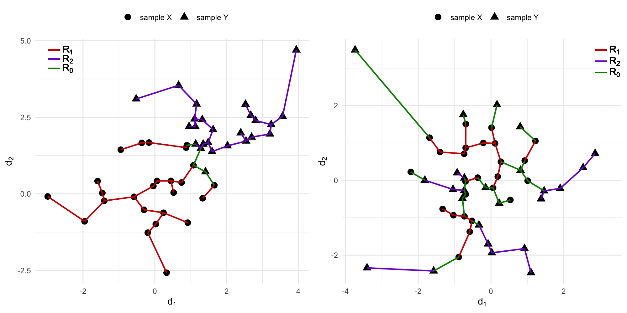
Figure 1. Computation of $R_{0}$, $R_{1}$, and $R_{2}$ for MST constructed on Euclidean distance. Left: The first 25 observations are generated from $\mathcal{N}((0,0)^{T},I_{2})$. The second 25 observations are generated from $\mathcal{N}((2,2)^{T},I_{2})$. Right: The first 25 observations are generated from $\mathcal{N}((0,0)^{T},I_{2})$. The second 25 observations are generated from $\mathcal{N}((0,0)^{T},1.5^{2}I_{2})$.

2.2. Hubness phenomenon in high-dimensional data

Hubs, defined to be nodes in the graph with a large degree, are a product of the the curse of dimensionality. The hubness phenomenon was carefully studied in [14], who showed that hubs are an inherent property of data distributions in high-dimensional and not an artifact of finite samples or specific data distributions. Their careful theoretical analysis showed that the probability that a hub emerges increases as the data dimension increases. The high-dimensional setting amplifies the tendency of central observations (observations close to the mean) to become hubs, effectively making it easier for an observation to become a ‘popular’ or ‘central’ node. As a result, $k$-MSTs and $k$-NNGs constructed on high dimensional data tend to have large hubs under standard distance measures, such as $L_{p}$. Hubs can be highly influential nodes and can distort final results depending on whether these nodes are included or excluded.

To see that the presence of hubs is a common phenomenon for high-dimensional data, we construct $5$-MST graphs using Euclidean distance and report their maximum node degrees. We run 100 simulations with $n_{1}=n_{2}=500$, where observations are drawn from multivariate standard normal and multivariate $t$ with $3$ degrees of freedom. For each simulation setting, we report the maximum node degree and 95th percentile of node degree; boxplots of these quantities are shown in Figure 2. We see that the 95th percentiles of node degrees are smaller than 40, but the maximum node degrees are more than three times as much as the 95th percentiles. Clearly it is not uncommon to have a node with a degree much larger than the majority of other nodes’ in the similarity graph. Observe that as the dimension increases, the max node degree also increases. This phenomenon is more pronounced in heavy-tailed distributions, such as the multivariate $t$-distribution.

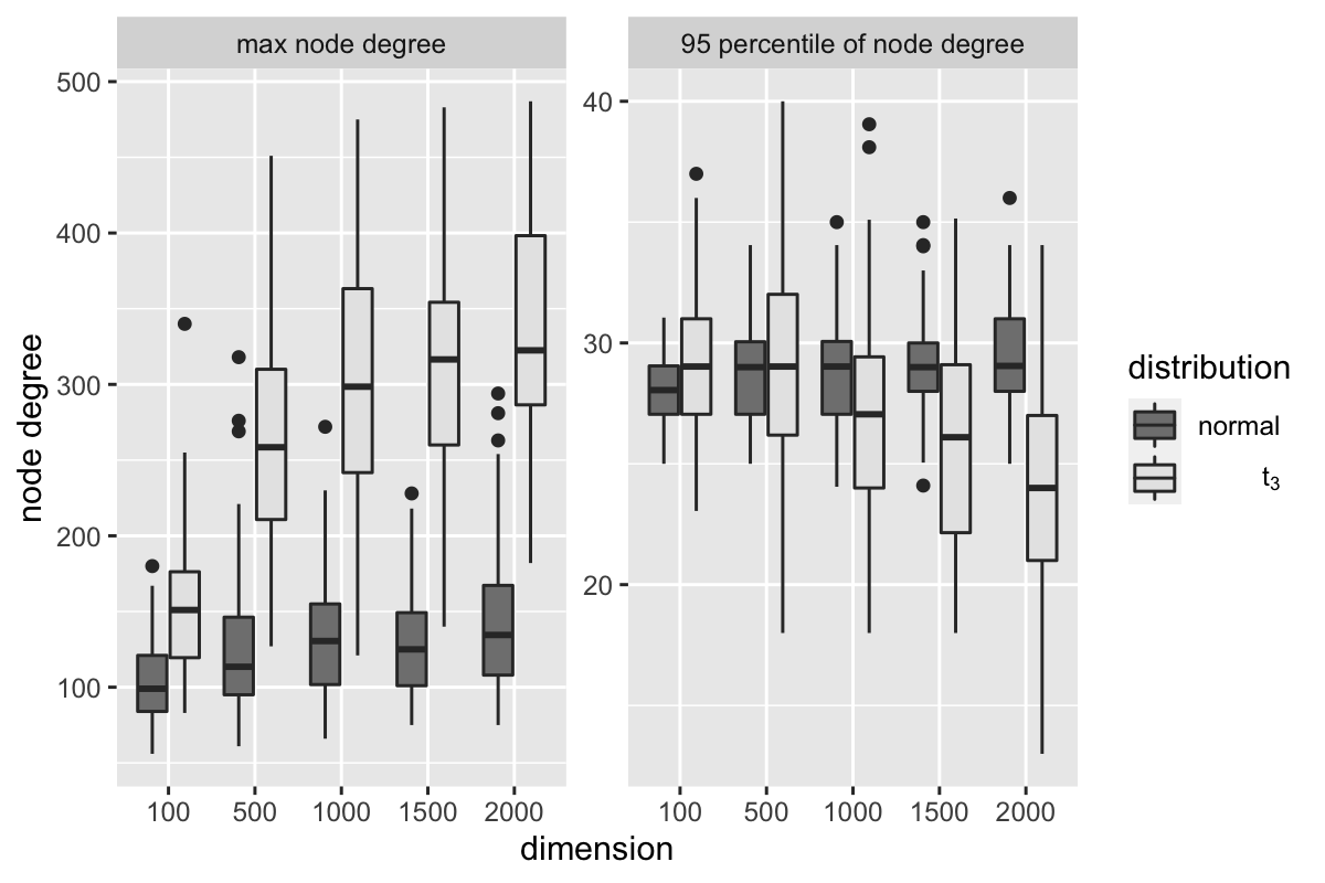
Figure 2. Boxplot of maximum node degrees and 95th percentiles of node degrees for different dimensions and distributions. Here $n_{1}=n_{2}=500$.

2.3. Limitations of current graph-based tests

In order to understand why large hubs may cause problems in the existing graph-based tests, let us consider the following example. We simulate observations from two distributions: Sample 1 $\sim\mathcal{F}_{1}:\mathcal{N}(\textbf{0},\textbf{I}_{500})$ and Sample 2 $\sim\mathcal{F}_{2}:\mathcal{N}(\boldsymbol{\mu},\big{(}\begin{smallmatrix}1.2^{2}\textbf{I}_{100}&\textbf{0}\\ \textbf{0}&\textbf{I}_{400}\end{smallmatrix}\big{)})$, where $||\boldsymbol{\mu}||=1$. In Scenario 1, 100 observations are generated from $F_{1}$ and $F_{2}$ respectively and a 5-MST is constructed based on Euclidean distance using the pooled observations. The maximum node degree in the graph is 71, and the graph is relatively flat. In Scenario 2, the observations are generated in the same manner, but one observation in Sample 2 is shifted toward the mean so that the 5-MST graph contains a hub with a node degree of 97. Moving towards the mean is a high-probability event and not an extreme scenario.

Since the type of alternatives in Scenario 1 and Scenario 2 involve both mean and scale change, the generalized edge-count test $S$ and the max-type edge-count test $M$ are recommended. These graph-based tests are powerful for detecting general distributional differences and were proposed in [5] and [7], respectively. Both tests involve using combinations of $R_{1}$ and $R_{2}$ and a large value of $S$ or $M$ is evidence against $H_{0}$. The performance of these two tests under Scenarios 1 and 2 are shown in Table 1. We can see both tests work perfectly well under Scenario 1, but are unable to reject the null hypothesis at 10% significance level in the presence of a hub (Scenario 2).

Table 1. Comparison of tests under Scenario 1 and Scenario 2

Test Type	Scenario 1		Scenario 2
	Test Statistic	p-value	Test Statistic	p-value
$S$	17.6591	0.0001	4.3331	0.1146
$M$	3.3433	0.0012	1.7645	0.1135

Table 2. Graph-based quantities for 5-MST under Scenario 1 and Scenario 2

Edge-count	Scenario 1			Scenario 2
	Value	Mean	Variance	Value	Mean	Variance
$R_{1}$	356	247.5	1150.937	322	247.5	1472.912
$R_{2}$	161	247.5	1150.937	189	247.5	1472.912

Table 2 sheds insight on why this happens. Two graph-based quantities $R_{1}$ and $R_{2}$ are reported. Recall that $R_{1}$ is the number of edges that connects observations within Sample 1 and $R_{2}$ is the number of edges that connects observations within Sample 2. Under the alternative, we would expect the absolute value of differences $R_{1}-E(R_{1})$ and $R_{2}-E(R_{2})$ to be relatively large. Here $E(R_{1})$ and $E(R_{2})$ denote the expectations of the respective edge-counts under the permutation null distribution.

Under Scenario 1, $R_{1}$ and $R_{2}$ behave as we expect: $R_{1}$ (356) is large relative to its expectation under the null (247.5) and $R_{2}$ (161) is small relative to its expectation under the null (247.5), therefore the differences between within sample edge counts and their expectations are relatively large. Under Scenario 2, two problems arise in the presence of a hub. First, observations from both samples tend to construct an edge with the hub. So, compared to Scenario 1, $R_{1}$ decreases (322) and $R_{2}$ increases (189). The relative differences between $R_{1}$ and $R_{2}$ with their respective null expectations then become smaller, causing both $S$ and $M$ to lose power.

Second, the variances of both $R_{1}$ and $R_{2}$ also increase, further inhibiting the power of the test statistics. Let $G$ denote the similarity graph and its set of edges, $|G|$ denote the number of edges in $G$, $G_{i}$ be the subgraph including all edge(s) that connect to node $i$, and $|G_{i}|$ be the degree of node $i$ in $G$. The symbol $(i,j)$ denotes an edge with endpoints $i$ and $j$ in graph $G$. This second problem can be clearly seen by studying the analytical expression of the variance of the edge-count, $R_{i}$, under the permutation null distribution:

$$\begin{split}Var(R_{j})=&\mu_{j}(1-\mu_{j})+2C\frac{n_{j}(n_{j}-1)(n_{j}-2)(N-n_{j})}{N(N-1)(N-2)(N-3)}+\\ &|G|(|G|-1)\frac{n_{j}(n_{j}-1)(n_{j}-2)(n_{j}-3)}{N(N-1)(N-2)(N-3)},\end{split}$$

where $j=1,2$, $\mu_{j}=E(R_{j})=|G|\frac{n_{j}(n_{j}-1)}{N(N-1)}$, $C=\frac{1}{2}\sum_{i=1}^{N}|G_{i}|^{2}-|G|$, $n_{j}$ is the number of observations in sample $j$, and $N=n_{1}+n_{2}$.

In the presence of a hub, $\sum_{i=1}^{N}|G_{i}|^{2}$ and $C$ increase, where $C$ represents the number of edge pairs sharing a common node. Since all the other terms remain the same under both scenarios, this results in an inflated variance for $R_{1}$ and $R_{2}$ in the presence of hubs.

2.4. Our Contribution

When the size or density of hubs is large, existing graph-based tests can suffer from limited power and unstable performance. That said, it can be tricky to identify every single hub that may cause problems. Instead of identifying ‘influential’ hubs, which can be data or application-specific, we propose new test statistics that are useful even in the presence of hubs. Specifically, we propose to apply appropriate weights to the test statistics that will dampen the effect of hubs while still retaining crucial similarity information. We show that these weights can improve power and resolve the variance boosting problem in the presence of hubs. We provide recommendations for weights as functions of node degrees and demonstrate that these work well in a range of scenarios. The limiting null distribution of these new robust test statistics are derived under mild conditions on the weights.

3. Robust edge-count test statistics

Let $d_{i}$ denote the node degree of node $i$ in a graph $G$. The graph $G$ is a similarity graph (such as a $k$-MST or $k$-NN, where $k$ is pre-specified). Our approach is to flatten the similarity graph, and limit the influence of hubs, without incurring too much of a loss of similarity information so that the testing procedure can still retain power. To do so, we propose to apply weights to the test statistic. The weights should be designed such that edges connected to a hub (a node with a large $d_{i}$) are down-weighted, while other edges are left mostly undisturbed. Formally, let $w_{ij}$ denote the weight on edge $(i,j)$ where $w_{ij}$ is the value of the weight function $W(d_{i},d_{j})$, with $W(d_{i},d_{j})$ defined to be a function of $d_{i}$ and $d_{j}$. Discussions about the choice of weight functions are deferred to Section 3.1.

We propose test statistics that apply weights $w_{ij}$ to the edge-counts $R_{0}(i,j)$, $R_{1}(i,j)$, and $R_{2}(i,j)$, such that each edge $(i,j)\in G$ is weighted by a combination of $d_{i}$ and $d_{j}$. Let $g_{i}=0$ if the observation $i$ is from Sample $\boldsymbol{X}$, and 1 otherwise. Let $n_{1}$ be the sample size of Sample $\boldsymbol{X}$, $n_{2}$ be the sample size of Sample $\boldsymbol{Y}$, and $N=n_{1}+n_{2}$. We define

$$J_{(i,j)} =\begin{cases}1&\text{if $g_{i}=g_{j}=0$},\\ 2&\text{if $g_{i}=g_{j}=1$},\end{cases}$$

$$R_{1}(i,j) =w_{ij}I(J_{(i,j)}=1),$$

$$R_{2}(i,j) =w_{ij}I(J_{(i,j)}=2),$$

$$R_{1}^{w} =\sum_{(i,j)\in G}R_{1}(i,j),$$

$$R_{2}^{w} =\sum_{(i,j)\in G}R_{2}(i,j).$$

The robust generalized edge-count test statistic is defined to be:

$$S_{R}=(R_{1}^{w}-\mu_{1}^{w},R_{2}^{w}-\mu_{2}^{w})(\Sigma^{w})^{-1}\begin{pmatrix}R_{1}^{w}-\mu_{1}^{w}\\ R_{2}^{w}-\mu_{2}^{w}\end{pmatrix},$$

where $\mu_{1}^{w}=E(R_{1}^{w}),\mu_{2}^{w}=E(R_{2}^{w})$, and

$$\Sigma^{w}=\begin{pmatrix}\textbf{Var}(R_{1}^{w})&\textbf{Cov}(R_{1}^{w},R_{2}^{w})\\ \textbf{Cov}(R_{1}^{w},R_{2}^{w})&\textbf{Var}(R_{2}^{w})\end{pmatrix}=\begin{pmatrix}\Sigma_{11}&\Sigma_{12}\\ \Sigma_{21}&\Sigma_{22}\end{pmatrix}.$$

Theorem 1.

$S_{R}$ can be expressed as

$$S_{R}=(Z^{R}_{\text{diff}})^{2}+(Z^{R}_{w})^{2},$$

with

$$\textbf{Cov}(Z^{R}_{\text{diff}},Z^{R}_{w})=0,$$

where $Z_{\text{diff}}^{R}=\frac{(R_{1}^{w}-R_{2}^{w})-\textbf{E}(R_{1}^{w}-R_{2}^{w})}{\sqrt{\textbf{Var}(R_{1}^{w}-R_{2}^{w})}}$, $Z_{w}^{R}=\frac{(qR_{1}^{w}+pR_{2}^{w})-\textbf{E}(qR_{1}^{w}+pR_{2}^{w})}{\sqrt{\textbf{Var}(qR_{1}^{w}+pR_{2}^{w})}}$, $p=\frac{n_{1}-1}{N-2}$, and $q=1-p$.

The proof can be found in the Appendix C.

Theorem 1 leads us to propose the robust max-type edge-count test statistic:

$$M_{R}=\text{max}(Z_{w}^{R},|Z_{\text{diff}}^{R}|).$$

If the graph is relatively flat and no hub is present, then $d_{i}$ is similar for all $i\in G$, and the weights have little effect. However, in the presence of a problematic hub(s), the weights control the influence of edges connected to the hub, resulting in improved performance. This makes the test statistic more robust to the underlying similarity graph and also resolves the variance boosting problem.

The analytic expressions of expectations and variances involved above can be obtained by combinatorial analysis under the permutation null distribution. The corresponding analytic expressions are given in Lemma 1.

Lemma 1.

Under the permutation distribution, we have:

$$\begin{split}\mu_{1}^{w}=&\sum_{(i,j)\in G}w_{ij}\frac{n_{1}(n_{1}-1)}{N(N-1)},\ \mu_{2}^{w}=\sum_{(i,j)\in G}w_{ij}\frac{n_{2}(n_{2}-1)}{N(N-1)},\\ \Sigma_{11}=&\left\{-S_{2}+\frac{2(2N-3)}{N(N-1)}S_{3}+\frac{N-3}{n_{2}-1}\left(S_{1}+S_{2}\right)-\frac{4(N-3)}{N(n_{2}-1)}S_{3}\right\}\times\\ &\frac{n_{1}n_{2}(n_{1}-1)(n_{2}-1)}{N(N-1)(N-2)(N-3)},\\ \Sigma_{22}=&\left\{-S_{2}+\frac{2(2N-3)}{N(N-1)}S_{3}+\frac{N-3}{n_{1}-1}\left(S_{1}+S_{2}\right)-\frac{4(N-3)}{N(n_{1}-1)}S_{3}\right\}\times\\ &\frac{n_{1}n_{2}(n_{1}-1)(n_{2}-1)}{N(N-1)(N-2)(N-3)},\\ \Sigma_{12}=&\left\{-S_{2}+\frac{2(2N-3)}{N(N-1)}S_{3}\right\}\frac{n_{1}n_{2}(n_{1}-1)(n_{2}-1)}{N(N-1)(N-2)(N-3)},\end{split}$$

where $S_{1}=\sum_{(i,j)\in G}w_{ij}^{2}$, $S_{2}=\sum_{(i,j),(i,k)\in G}w_{ij}w_{ik}$ and $S_{3}=\sum_{(i,j),(k,l)\in G}w_{ij}w_{kl}$.

The proof to this lemma can be found in the Appendix A.

Using the results from Lemma 1, the expectations and variances involved in $Z_{\text{diff}}^{R}$ and $Z_{w}^{R}$ can be obtained as follows:

$$\textbf{E}(R_{1}^{w}-R_{2}^{w}) = \sum_{(i,j)\in G}w_{ij}\frac{n_{1}-n_{2}}{N},$$

$$\textbf{E}(q_{w}R_{1}^{w}+p_{w}R_{2}^{w}) = \sum_{(i,j)\in G}w_{ij}\frac{(n_{1}-1)(n_{2}-1)}{(N-1)(N-2)},$$

$$\textbf{Var}(R_{1}^{w}-R_{2}^{w}) = \left\{(S_{1}+S_{2})-\frac{4}{N}S_{3}\right\}\frac{n_{1}n_{2}}{N(N-1)},$$

$$\textbf{Var}(q_{w}R_{1}^{w}+p_{w}R_{2}^{w}) = \left\{\frac{N-3}{N-2}S_{1}-\frac{1}{N-2}S_{2}+\frac{2}{(N-1)(N-2)}S_{3}\right\}\times$$

$$\frac{n_{1}n_{2}}{N(N-1)}\frac{(n_{1}-1)(n_{2}-1)}{(N-2)(N-3)}.$$

Large values of $S_{R}$ and $M_{R}$ are evidence against the null hypothesis of no distributional difference. The construction of both $S_{R}$ and $M_{R}$ allow them to be powerful for general alternatives. When there is a change in mean, both $R_{1}^{w}$ and $R_{2}^{w}$ tend to be large, and then $Z^{R}_{w}$ will be large, which leads to a large $S_{R}$ and $M_{R}$. When a change in variance is present, without loss of generality, suppose the sample with the smaller variance is sample $\boldsymbol{X}$, then $R_{1}^{w}$ is relatively large compared to its null expectation while $R_{2}^{w}$ is relatively small. In this case, $|Z^{R}_{\text{diff}}|$ tends to be large which also leads to a large $S_{R}$ and $M_{R}$.

Remark 1.

The test statistics are well-defined under the following conditions:

1. $\sum_{\{j,\text{s.t.}(i,j)\in G\}}w_{ij}$ are not all equal for all $i\in[1,N]$,

2. $(N-3)S_{1}-S_{2}+\frac{2}{N-1}S_{3}>0$,

where $S_{1}=\sum_{(i,j)\in G}w_{ij}^{2}$, $S_{2}=\sum_{(i,j),(i,k)\in G}w_{ij}w_{ik}$ and $S_{3}=\sum_{(i,j),(k,l)\in G}w_{ij}w_{kl}$.

The proof to this remark can be found in the Appendix B.

For example, for a completely flat graph (all nodes have the same degree), then $w_{ij}=w_{i^{\prime},j^{\prime}},\ \forall i,j$ and $Z_{\text{diff}}$ is not well-defined. For a star-shaped graph (all observations connect to the same node), $Z_{w}$ is not well-defined.

The robust test statistics $S_{R}$ and $M_{R}$ default to the tests proposed in [5] and [7] when $w_{ij}=1$ for all $(i,j)$. In [5] and [7], each edge has an equal contribution to the test statistic so that even those edges connected to problematic hubs are treated with the same weight as those that are not. By placing weights on the edges, we dampen the influence of hubs and effectively flatten the graph. The weights $w_{ij}$ must be positive and bounded (asymptotically) below by $1/|G|$. Theorem 2 ensure $R_{k}^{w},k=1,2$ does not vanish to zero when the sample size goes to infinity.

Theorem 2.

Let $W$ be a weight function such that $W(i,j)=w_{ij}$ for all edges $(i,j)$. If the weight function $1/|G|\precsim W$ then $\lim_{N\to\infty}R_{k}^{w}>0$.

The proof to this theorem can be found in the Appendix D.

3.1. Choice of Weights

The test statistics are defined for general weights that are functions of the node degrees and monotonically decreasing, as defined below.

Definition 1.

A bivariate function is called monotonically decreasing (or non-increasing), if for all $x_{1}$, $x_{2}$ and $y_{0}$ such that $x_{1}<x_{2}$ one has $f(x_{1},y_{0})>f(x_{2},y_{0})$; and for all $y_{1}$, $y_{2}$ and $x_{0}$ such that $y_{1}<y_{2}$ one has $f(x_{0},y_{1})>f(x_{0},y_{2})$.

In practice, users have the flexibility to choose their weights, provided that the test statistics are well-defined following conditions in Remark 1. Since we allow the graph to be general (it could be MST, NNG, or based on domain-knowledge), and the weights are properties of the graph, this makes obtaining optimal weights for general graph construction challenging. We reserve this line of theoretical analysis for future work. In this paper, we provide recommendations for weights based on empirical studies. We recommend weights that (1) demonstrate reasonable power and (2) meet the conditions for our asymptotic theory. In particular, we study the performance of three weight functions and show that they work well in a variety of settings.

For edge $(i,j)$, we consider the following weight functions:

$$W_{1}(d_{i},d_{j}) =\frac{1}{\text{max}(d_{i},d_{j})},$$

$$W_{2}(d_{i},d_{j}) =\frac{1}{\sqrt{d_{i}d_{j}}},$$

$$W_{3}(d_{i},d_{j}) =\frac{2}{(d_{i}+d_{j})}.$$

The weight function $W_{1}$ returns the inverse of the max node degree of an edge $(i,j)$. The weight functions $W_{2}$ and $W_{3}$ take the inverse of the arithmetic average and the geometric average of the node degrees of an edge, respectively. All three weight functions are bounded below by $1/|G|$ asymptotically and monotonically decreasing.

To have a better understanding of the weight functions, we plot the three weights for increasing node degrees in Figure 3. For a given edge ($i,j$), we fix $d_{i}$ to be $5$ and increase $d_{j}$ from 5 to 200. We can see weight function $W_{1}$ gives the heaviest penalty. When the max node degree is larger than 100, the weight function $W_{1}$ and $W_{3}$ provide similar weights. The weight function $W_{2}$ gives a milder penalty on node degrees among these three weight functions.

Figure 3. Comparison of weight functions

To more comprehensively evaluate the performance of these three weight functions, we simulate data with $n_{1}=n_{2}=100$ and $d=200$ from a $d$-dimensional Gaussian distribution under both mean and scale change. The similarity graph is a $5$-MST constructed from Euclidean distance. We consider ten scenarios with increasing hub sizes. Each scenario consists of 100 trials. For each trial, the max node degree is recorded and boxplots under each scenario are shown in Figure 4. From scenario 1 to 10, the maximum node degree increases, so the hub connects to more observations, resulting in a bigger impact on the similarity graph. The number of trials with significance less than 5% under 10,000 permutations in each scenario is shown in Figure 5 and 6.

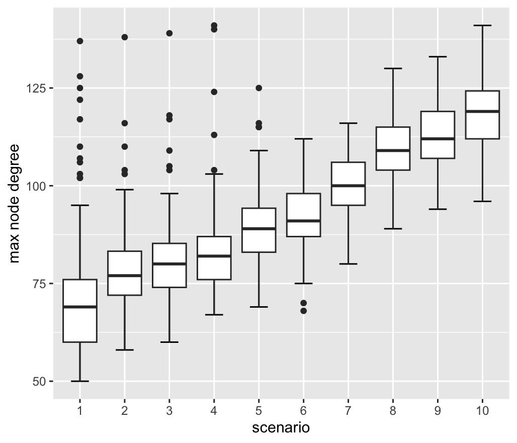
Figure 4. Boxplot of the max node degrees under each scenario

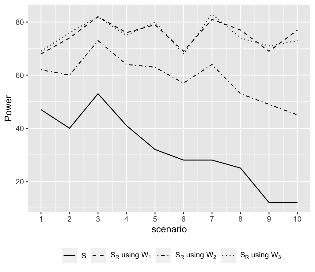
Figure 5. Power comparison of $S$ and $S_{R}$ using different weight functions. Y axis represents number of trials (out of 100) with significance less than 5%

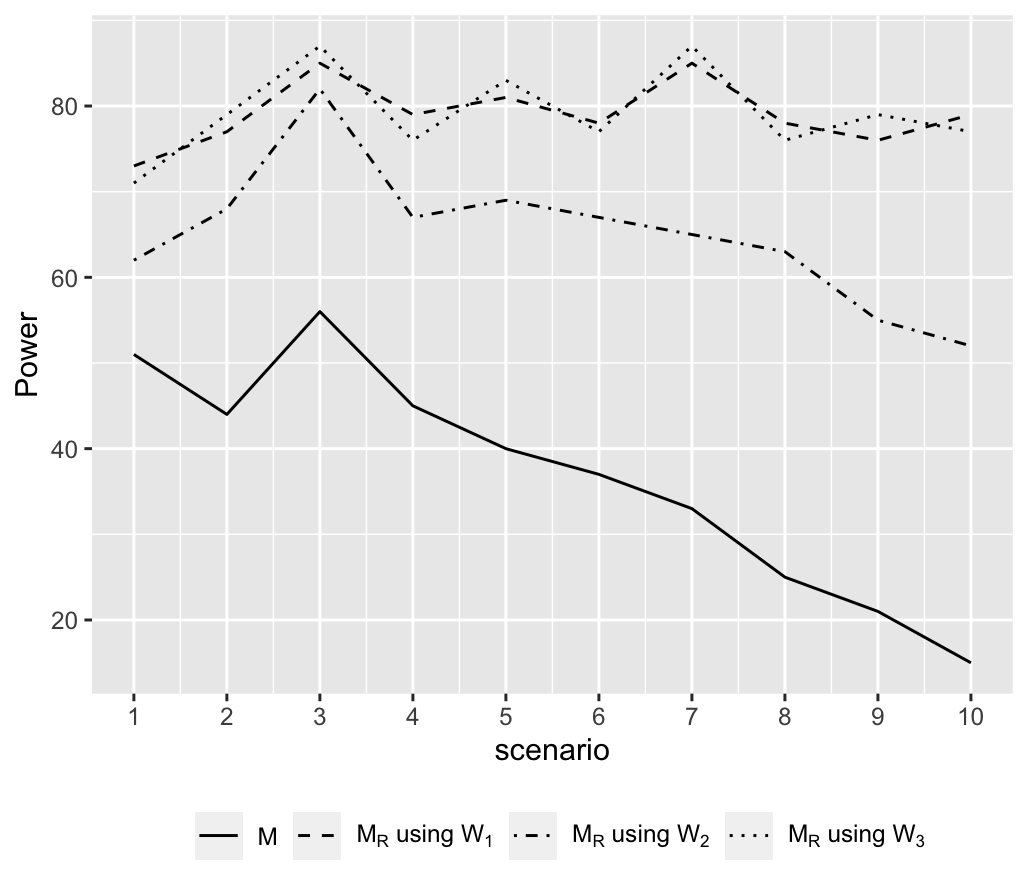
Figure 6. Power comparison of $M$ and $M_{R}$ using different weight functions. Y axis represents number of trials (out of 100) with significance less than 5%

It is clear all three weighted test statistics outperform their non-weighted counterparts. Weight functions $W_{1}$ and $W_{3}$ have similar power and tend to dominate across all scenarios. On the other hand, the weight function $W_{2}$ does not have enough weight to resist the impact of the hub and has slightly lower power across all scenarios compared to $W_{1}$ and $W_{3}$. This is because $W_{2}$ is unable to counteract the variance boosting problem as effectively as $W_{1}$ and $W_{3}$. As shown in Figure 7, the variances of $R_{1}^{w}$ and $R_{2}^{w}$ are well controlled for $W_{1}$ and $W_{3}$, but for $W_{2}$ the variance grows as the max node degree grows.

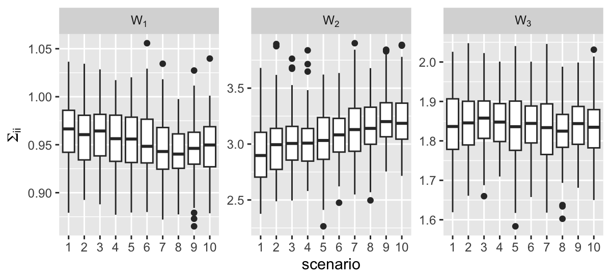
Figure 7. Boxplots of $\Sigma_{ii},i=1,2$ under each scenario for weight functions $W_{1}$, $W_{2}$ and $W_{3}$.

In what follows, we recommend using the weight function $W_{1}$ or $W_{3}$. We discuss how these weights satisfy our conditions for obtaining the limiting null distribution in Section 4.

4. Asymptotic Results

4.1. Asymptotic null distribution of the robust test statistics

When the sample size is small, we can obtain $p$-values for the test statistics by resampling from the permutation distribution. However, as the sample size increases, this becomes computationally prohibitive. To make the tests practical for modern data sets, we study the limiting distributions of the robust edge-count test statistics.

We define

• $A_{(i,j)}=\{(i,j)\}\cup\{(i^{\prime},j^{\prime})\in G,(i,j)$ and $(i^{\prime},j^{\prime})$ share a node},

• $B_{(i,j)}=A_{(i,j)}\cup\{(i^{\prime\prime},j^{\prime\prime})\in G,\exists(i^{\prime},j^{\prime})\in A_{(i,j)}$, such that $(i^{\prime},j^{\prime})$ and $(i^{\prime\prime},j^{\prime\prime})$ share a node},

• $W(A_{(i,j)})=\sum_{(i^{\prime},j^{\prime})\in A_{(i,j)}}w_{i^{\prime}j^{\prime}}$,

• $W(B_{(i,j)})=\sum_{(i^{\prime\prime},j^{\prime\prime})\in B_{(i,j)}}w_{i^{\prime\prime}j^{\prime\prime}}$.

Theorem 3.

Under conditions

1. $G=\mathcal{O}(N^{\alpha}),1\leq\alpha<1.25$,

2. $S_{1}+S_{2}-\frac{4}{N}S_{3}=\mathcal{O}(S_{1}+S_{2})$,

3. $\sum_{(i,j)\in G}(w_{ij}|A_{(i,j)}|)^{2}=o(S_{1}\sqrt{N})$,

4. $\sum_{(i,j)\in G}w_{ij}W(A_{(i,j)})W(B_{(i,j)})=o(S_{1})^{1.5}$,

as $n_{1}$, $n_{2}$, $N\rightarrow\infty$ and $n_{1}/N\rightarrow\lambda\in(0,1)$, $Z_{w}^{R}\xrightarrow{\mathcal{D}}N(0,1)$ and $Z_{\text{diff}}^{R}\xrightarrow{\mathcal{D}}N(0,1)$ under the permutation null distribution.

The proof utilizes Stein’s theorem from [6], and details are provided in the Supplementary Material Section E.

Corollary 1.

Under conditions in Theorem 3, as $n_{1},n_{2},N\rightarrow\infty$ and $n_{1}/N\rightarrow\lambda\in(0,1)$, $S_{R}\xrightarrow{\mathcal{D}}\chi_{2}$ under the permutation null distribution.

Condition (ii) ensures $Z^{R}_{\text{diff}}$ is asymptotically well-defined. Conditions (iii) and (iv) prevent the sum of weights in the hub from growing too large.

To see that the conditions hold easily in the presence of hubs, we generated data from Gaussian distribution as well as the heavy-tailed $t_{5}$ distribution and construct $5$-MST from Euclidean distance. Ratios of the key quantities involved in the conditions using 5-MST are shown in Figure 8. Once we assign weights, the ratios $\sum(w_{ij}|A_{(i,j)}|)^{2}/(S_{1}\sqrt{N})$ and $(\sum w_{ij}W(A_{(i,j)})W(B_{(i,j)})/(S_{1})^{1.5}$ are bounded by $o(1)$ under all scenarios for both $W_{1}$ and $W_{3}$.

Figure 8. Ratios of key quantities. Data are generated from $d$-dimensional Normal and $t_{5}$ distributions. Graphs are constructed based on 5-MST. Left: the ratio of $\sum(w_{ij}|A_{(i,j)}|)^{2}$ to $S_{1}N^{0.5}$. Right: the ratio of $\sum w_{ij}W(A_{(i,j)})W(B_{(i,j)})$ to $(S_{1})^{1.5}$.

To assess the performance for finite sample sizes, we compare the critical values generated from the 10,000 permutations with the critical values obtained from asymptotic results under the null hypothesis. The data are generated from log-normal and $t_{5}$ distributions with $n_{1}=n_{2}=50$ and $d=100$. The graphs are generated using 5-MST with Euclidean distance. The boxplots of the differences between asymptotic critical values and permutation critical values using different weight functions are shown in Figure 9. The p-value approximations are reasonable based on small differences shown in the boxplots.

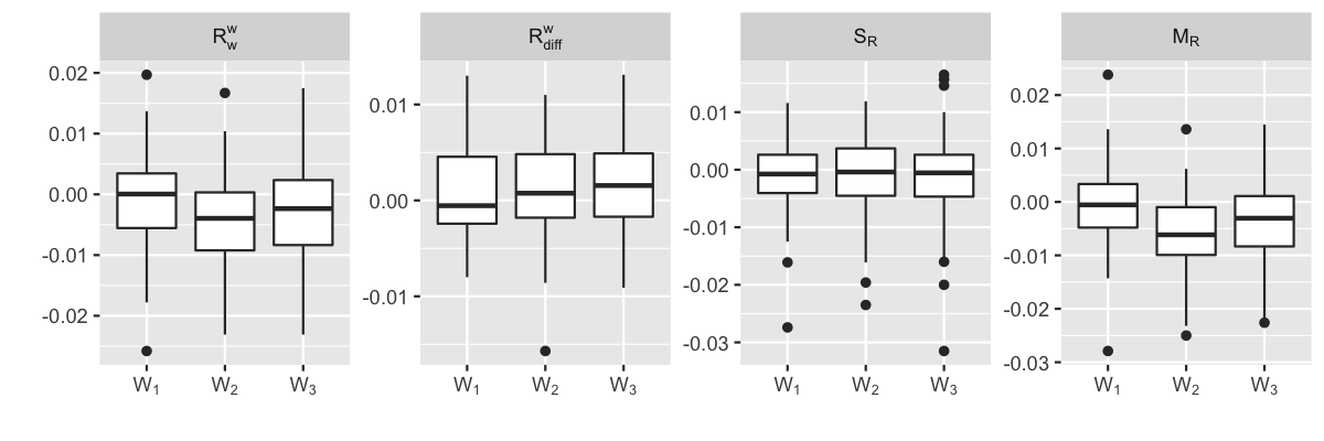
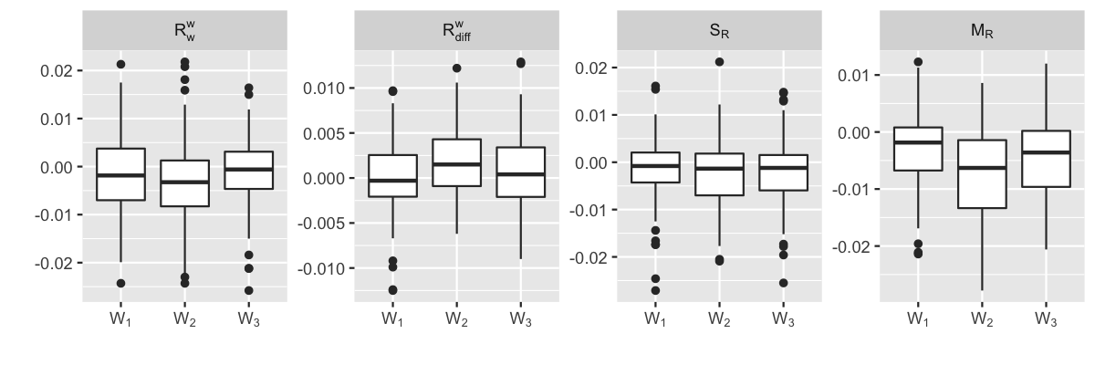
Figure 9. Boxplots of differences between asymptotic critical values and permutation critical values. $R_{w}^{w}=qR_{1}^{w}+pR_{2}^{w}$, $R_{\text{diff}}^{w}=R_{1}^{w}-R_{2}^{w}$. Upper row: log-normal distribution. Lower row: $t_{5}$ distribution.

5. Performance Analysis

5.1. Hubs in high-dimensional data

We examine the performance of the robust test statistics on high-dimensional data, which tend to contain hubs. We set $n_{1}=n_{2}=100$. The similarity graph is the 5-MST constructed from $L_{2}$ distances of the pooled observations. We present the power of the tests, which is estimated to be the number of trials (out of 100) with significance less than 5%. We also report median of the max node degrees in each trial (over 100 trials), denoted as $\tilde{d}_{\text{max}}$.

Table 3 shows results for log-normal data differing in location parameter $\mu$, which results in both mean and variance differences between the two samples. The change is denoted by $\Delta_{\mu}$ and is selected so that all the tests have moderate power. As the dimension increases, and the maximum node degree subsequently increases, the robust edge-count tests out-perform their non-weighted counterparts. The improvement of the robust edge-count tests are more noticeable in the heavy-tail $t$ distribution. As shown in Table 4, $\Delta_{v}$ denotes the change in degrees of freedom compared to degrees of freedom $v=5$ and $\Delta_{\mu}$ denotes the change in non-centrality parameter in a $d$-dimensional non-central $t$ distribution.

Table 3. Number of trials (out of 100) with significance less than 5%. Data generated from multivariate log-normal distribution.

			Test-statistic
d	$\Delta_{\mu}$	$\tilde{d}_{\text{max}}$	$S$	$S_{R}$		$M$	$M_{R}$
			$W_{1}$	$W_{3}$		$W_{1}$	$W_{3}$
200	1.7	120	78	78	78	76	83	84
500	1.9	156	59	73	74	66	78	82
1000	2.5	175.5	75	90	91	79	94	93
1500	2.7	182.5	74	91	92	72	93	92

Table 4. Number of trials (out of 100) with significance less than 5%. Data generated from multivariate non-central $t$ distribution.

				Test-statistic
d	$\Delta_{\mu}$	$\Delta_{v}$	$\tilde{d}_{\text{max}}$	$S$	$S_{R}$		$M$	$M_{R}$
				$W_{1}$	$W_{3}$		$W_{1}$	$W_{3}$
200	0.8	1	85	71	86	86	72	90	89
500	1	0.5	96	48	74	74	56	79	76
1000	1.5	0.4	108.5	61	82	80	60	87	87
1500	2	0.3	106	63	84	81	65	85	84

5.2. Hub generated from influential observations

In this section, we will study how the tests behave when a single observation generates a hub; consider this observation an influential point. The setup is as follows: for each trial, the two samples are generated from $d$-dimensional Gaussian distributions that differ in both mean and variance with $n_{1}=n_{2}=100$. The mean difference (in $L_{2}$ distance) of the two samples is denoted by $\Delta_{\mu}$ and the ratio between the standard deviations is denoted by $\rho_{\sigma}$.

Then one observation from the sample with a larger variance (sample 2) is replaced by an influential point that induces a hub, and the influential point is generated from the same distribution as other observations in sample 2. The results are reported in Table 5.

For Table 5 , the robust tests using $W_{1}$ and $W_{3}$ tend to have similar power. When there is an influential observation, the edge-count tests $S$ and $M$ suffer from lower power while the robust edge-count test statistics, $S_{R}$ and $M_{R}$, still provide reasonable performance.

Table 5. Number of trials (out of 100) with significance less than 5%. Multivariate Gaussian data with influential observation.

				Test-statistic
d	$\Delta_{\mu}$	$\rho_{\sigma}$	$\tilde{d}_{\text{max}}$	$S$	$S_{R}$		$M$	$M_{R}$
				$W_{1}$	$W_{3}$		$W_{1}$	$W_{3}$
50	0.1	1.08	84	55	93	91	58	94	92
100	0.2	1.06	99.5	47	98	98	54	99	100
150	0.3	1.04	92.5	31	89	89	35	93	92
200	0.6	1.038	92	60	96	95	60	97	97
250	0.8	1.035	99.5	57	95	94	59	99	98

6. Real Data Application

We illustrate the robust graph-based tests on Chicago taxi trip dataset. This data is publicly available on the Chicago Data Portal website (https://data.cityofchicago.org/Transportation/Taxi-Trips/wrvz-psew) and includes pick-up and drop-off dates, times, and locations for each taxi trip. The pickup and drop-off locations are recorded as the center of the census tract or the community area if the census tract has been hidden for privacy. In this study, we focus on the taxi trips in 2020. There are 563 unique pick-up locations and 635 unique drop-off locations. Via an initial data inspection, we find that taxis appear to be less active between midnight and 5 am. The frequency of taxi trips also appears to vary from month to month; the most notable difference can be observed when comparing January - March to the rest of the year. This is due to the fact that the statewide stay-at-home order signed by the Illinois Governor took effect on March 21 in response to the spread of COVID-19. Taxi rides were scattered all over Chicago and the most popular spots are around Downtown Chicago and O’Hare International Airport. For most of the census tracts away from Downtown Chicago, the number of taxi rides is relatively small.

We count the frequency of taxi pickups and drop-offs in each location for a specified time interval. We analyze taxi pickups and drop-offs separately. Each pick-up observation is a $563\times 1$ vector of taxi trip counts for a time unit, where each element represents a unique pick-up location. For example, if the time unit is days, then the pick-up observation is the frequency of taxi pick-ups across various locations for a given day. The drop-off observations are defined similarly.

When constructing the matrices, many entries would be 0 or 1 since the taxi rides may not happen or only happen rarely in some locations for a given period. With such sparse count matrices, a hub with a large node degree is likely to arise. These hubs become problematic in the two-sample tests, and since the type of change is not specified, it is difficult to identify problematic observations just by examining the raw data. We will demonstrate that the robust edge-count test can circumvent this problem and lead to reasonable results even in the presence of sparse, high-dimensional taxi cab data.

To illustrate the new tests, we consider three different scenarios and compare the performance of the new tests with existing methods. In Scenario I and II, we consider taxi trips in a time interval (i.e. 5 - 9 am for each day), whereas in Scenario III, we consider taxi trips in a specific hour. The similarity graphs, $5$-MST, are constructed from the frequency of taxi trips across different locations based on $L_{1}$ distances, with each node representing the counts for a time unit. For this application, the robust edge-count tests are constructed using weight function $W_{1}$. For all tests, p-values are obtained via 10,000 permutations.

6.1. Scenario I

We compare taxi rides during morning rush hour, defined as 5 - 9 am, for November versus December. Results are shown in Table 6, where $d_{max}$ denotes the maximum node degree, and $\sum_{i=1}^{N}G_{i}^{2}$ and $C$ (described in Section 2.3) reflect the structural features of the similarity graph. Pick-ups and drop-offs are analyzed separately.

Table 6. P-values of the edge-count tests based on 10,000 permutations. Tests compare taxi trip records from 5 am to 9 am in November to trip records from 5 am to 9 am in December. The p-values smaller than 0.1 are bolded.

	$d_{max}$	$\sum_{i=1}^{N}G_{i}^{2}$	$C$	$S$	$M$	$S_{R}$	$M_{R}$
Pick-up	34	7306	3353	0.1227	0.1400	0.0316	0.0221
Drop-off	22	6940	3170	0.1533	0.1500	0.0217	0.0159

From Table 6, we see that the existing tests ($S$ and $M$) are unable to reject the null, while the robust tests have power to do so. The observation which generates the node with maximum node degree is November 23, 2020, the day before Thanksgiving, for both pick-ups and drop-offs. This hub is highly influential to our results and as a sanity check, we evaluate our results without the November 23 observation. After removing this observation, the p-values of edge-count tests are shown in Table 7; we see that without the presence of this hubs all the tests reject the null hypothesis and conclude that taxi rides in November and December are significantly different. Observe that the maximum node degree of 5-MST after removing the Nov. 23 observation decreases for the taxi pick-ups. For the drop-off data, the maximum node degree does not change much after removing the observation from November 23, but the structure of the graph changes such that most nodes with large node degrees are from observations in December, instead of November. The quantities $\sum_{i=1}^{N}G_{i}^{2}$ and $C$ decrease for both pick-ups and drop-offs, which means the hubness subsides when removing the influential observation.

Table 7. P-values of the edge-count tests based on 10,000 permutations. Tests compare taxi trip records from 5 am to 9 am in November and December after removing taxi rides on November 23.

	$d_{max}$	$\sum_{i=1}^{N}G_{i}^{2}$	$C$	$S$	$M$	$S_{R}$	$M_{R}$
Pick-up	21	6760	3085	0.0021	0.0046	0.0038	0.0041
Drop-off	20	6724	3067	0.0390	0.0496	0.0121	0.0123

In this scenario, there appears to be potentially only one highly influential observation that can lead to unstable results in existing tests, while the new edge-count tests demonstrate robustness against this observation.

6.2. Scenario II

In the early morning hours (12 am - 6 am), the number of taxi rides is quite small compared to the daytime; this sparsity makes it easier to induce hubs with large node degrees when constructing the 5-MST. We compare taxi drop-offs during the early morning hours (12 am - 6 am) for April versus May, immediately after the lockdown was announced. The robust edge-count tests ($S_{R},M_{R}$) and the non-weighted versions ($S$, $M$) result in conflicting conclusions at $10\%$ significance level (Table 8). We see that for taxi drop-offs, $S$ and $M$ cannot reject the null, while the robust tests, $S_{R}$ and $M_{R}$, provide evidence of a difference between travel patterns in the two samples.

Table 8. P-values of the edge-count tests based on 10,000 permutations. Tests compare taxi trip records from 12 am to 6 am in April versus May. The p-values smaller than 0.1 are bolded.

	$d_{max}$	$S$	$M$	$S_{R}$	$M_{R}$
Drop-off	39	0.3423	0.1738	0.0306	0.0277

The existing tests ($S$ and $M$) are highly sensitive to the inclusion and exclusion of specific observations and can suffer from low power in the presence of a hub. The distribution of node degrees for the 5-MST is shown in Table 9. The observation generating the node with max node degree is from May 11. As shown in Table 10, after removing taxi trips on May 11, the generalized test ($S$) still cannot reject the null while $M$ can reject the null, leading to conflicting results among even the existing tests. On the other hand, removing the observation on May 18 (with a moderately large node degree of 17) leads to significant test results for both $S$ and $M$. Similarly, removing the observation representing taxi drop-offs on April 29 (with node degree 28), leads to significant test results for both $S$ and $M$.

Table 9. Distribution of node degrees in 5-MST generated from taxi drop-offs in April and May.

node degree	$<10$	10	11	12	13	14	15	16	17	19	20	26	27	28	39
frequency	42	2	1	4	2	1	1	1	1	1	1	1	1	1	1

Table 10. Results for the two-sample test comparing taxi drop-offs in April versus May after removing observations. We report the observation’s date, their node degree $d$, the number of edges connecting to observations from the same sample and the different sample, and the p-values after removing the observation on the specified date. The p-values smaller than 0.1 are bolded.

date	$d$	number of edges		p-value
		same	different	$S$	$M$	$S_{R}$	$M_{R}$
May 11	39	17	22	0.2020	0.0857	0.0645	0.0428
May 18	17	6	11	0.0787	0.0252	0.0084	0.0064
April 29	28	19	9	0.0153	0.0084	0.0071	0.0078

In this scenario, the inclusion and exclusion of specific observations may lead to unstable or conflicting results. On the other hand, the robust edge-count statistics provide more stable and consistent results.

6.3. Scenario III

We hereby present a scenario wherein the discernment of the problematic or influential observation becomes challenging. Table 11 shows edge-count test results for testing taxi rides from 12 am to 6 am in May versus June. Under scenario III, we count the taxi rides every hour, so the pooled pick-up and drop-off data are a $366\times 563$ matrix and a $366\times 635$ matrix, respectively. As shown in the table, $S$ and $M$ cannot reject the null at $10\%$ significance level for both taxi pick-ups and drop-offs, while the robust tests draw the opposite conclusion.

Table 11. P-values of the edge-count tests based on 10,000 permutations. Tests compare 12 am - 6 am taxi trip records between May and June. The p-values smaller than 0.1 are bolded.

	$d_{max}$	$S$	$M$	$S_{R}$	$M_{R}$
Pick-up	74	0.8793	0.6818	0.0116	0.0135
Drop-off	81	0.4251	0.2313	0.0075	0.0279

As a sanity check, we checked individual tests comparing taxi rides between May and June for each hour from 12 am to 6 am. As shown in Table 12 and Table 13, the null hypothesis that taxi rides in May and June are from the same distribution is rejected for the first two hours, and the smallest p-values, which appear in the test of taxi rides between 12 am to 1 am, are less than 1%. This can be considered as evidence that taxi rides from 12 am and 6 am are different in May and June, which suggests that the results of edge-count tests $S$ and $M$ in Table 11 suffer from low power.

Table 12. P-values of the edge-count tests based on 10,000 permutations. Tests compare one-hour taxi pick-up records from 12 am to 6 am between May and June. The p-values smaller than 0.1 are bolded.

	Pick-up
hour ( am )	$S$	$M$	$S_{R}$	$M_{R}$
12 - 1	$\mathbf{<0.0001}$	$\mathbf{<0.0001}$	$\mathbf{<0.0001}$	$\mathbf{<0.0001}$
1 - 2	0.0016	0.0075	0.0089	0.0408
2 - 3	0.2043	0.6474	0.1058	0.4711
3 - 4	0.5574	0.4254	0.1043	0.0528
4 - 5	0.2370	0.3271	0.4484	0.3478
5 - 6	0.1290	0.0545	0.0358	0.0225

Table 13. P-values of the edge-count tests based on 10,000 permutations. Tests compare one-hour taxi drop-off records from 12 am to 6 am between May and June. The p-values smaller than 0.1 are bolded.

	Drop-off
hour ( am )	$S$	$M$	$S_{R}$	$M_{R}$
12 - 1	$\mathbf{<0.0001}$	$\mathbf{<0.0001}$	$\mathbf{<0.0001}$	$\mathbf{<0.0001}$
1 - 2	0.0080	0.0113	0.0200	0.0488
2 - 3	0.2177	0.2350	0.2874	0.3586
3 - 4	0.2614	0.1145	0.2172	0.1318
4 - 5	0.2163	0.2619	0.6679	0.5779
5 - 6	0.4305	0.2988	0.7926	0.6540

7. Conclusion

We propose robust edge-count two-sample tests that address an aspect of the curse of dimensionality - the tendency of high-dimensional datasets to contain hubs. This tendency manifests itself in graph-based tests when constructing similarity grabs. We can consider observations that induce hubs can be treated as influential or outliers and their inclusion/exclusion in the analysis can lead to conflicting or unstable results. Our proposed robust edge-count tests mitigates this problem and can outperform the existing edge-count tests in the presence of the hubs while providing comparable power even when the graph is relatively flat. The robust edge-count tests are constructed by applying weights that are functions of node degrees to the edge-counts. Specific weight functions with desirable properties are recommended. We reserve designing an optimal graph-based weights for generic graphs as a topic worthy for future study.

The asymptotic permutation null distributions of the robust test statistics are given under some mild conditions on the weights. These conditions are shown through numeric studies to be easily satisfied even for heavy-tailed distributions in the presence of hubs. The $p$-value approximations based on asymptotic results are reasonably close to the permutation $p$-value for finite sample size, making the approach easy to apply to large data sets.

Simulation studies show that the robust edge-count tests have power gains over existing edge-count tests in high dimensions, since hubs are more easily generated as the dimension increases. The improvement is significant when the hub is generated from an influential point. An application of the tests on taxi data in Chicago demonstrate the robust test statistics utility in sparse, high-dimensional settings.

Appendix A Proof of Lemma 1

The mean and variance of $R_{1}^{w}$ under the permutation null distribution can be derived as follows:

$$\begin{split}\mu_{1}^{w}=&\sum_{(i,j)\in G}w_{ij}P(J_{(i,j)}=1)=\sum_{(i,j)\in G}w_{ij}\frac{n_{1}(n_{1}-1)}{N(N-1)},\\ E((R_{1}^{w})^{2})=&\sum_{(i,j),(k,l)\in G}w_{ij}w_{kl}P(J_{(i,j)}=1,J_{(k,l)}=1)\\ =&S_{1}\frac{n_{1}(n_{1}-1)}{N(N-1)}+S^{\prime}_{2}\frac{n_{1}(n_{1}-1)(n_{1}-2)}{N(N-1)(N-2)}+S^{\prime}_{3}\frac{n_{1}(n_{1}-1)(n_{1}-2)(n_{1}-3)}{N(N-1)(N-2)(N-3)},\\ \Sigma_{11}=&E((R_{1}^{w})^{2})-E^{2}(R_{1}^{w}),\end{split}$$

where

$$S_{1} =\sum_{(i,j)\in G}w_{ij}^{2},$$

$$S^{\prime}_{2} =\sum_{\begin{subarray}{c}(i,j),(i,k)\in G\\ k,l\text{ are different}\end{subarray}}w_{ij}w_{ik},$$

$$S^{\prime}_{3} =\sum_{\begin{subarray}{c}(i,j),(k,l)\in G\\ i,j,k,l\text{ all different}\end{subarray}}w_{ij}w_{kl}.$$

Similarly, we can get the mean and variance of $R_{2}^{w}$ under the permutation null distribution:

$$\begin{split}\mu_{2}^{w}=&\sum_{(i,j)\in G}w_{ij}P(J_{(i,j)}=2)=\sum_{(i,j)\in G}w_{ij}\frac{n_{2}(n_{2}-1)}{N(N-1)},\\ E((R_{2}^{w})^{2})=&S_{1}\frac{n_{2}(n_{2}-1)}{N(N-1)}+S^{\prime}_{2}\frac{n_{2}(n_{2}-1)(n_{2}-2)}{N(N-1)(N-2)}+S^{\prime}_{3}\frac{n_{2}(n_{2}-1)(n_{2}-2)(n_{2}-3)}{N(N-1)(N-2)(N-3)}\\ \Sigma_{22}=&E((R_{2}^{w})^{2})-E^{2}(R_{2}^{w}).\end{split}$$

The covariance of $R_{1}^{w}$ and $R_{2}^{w}$ under the permutation null distribution can be derived as follows:

$$\begin{split}E(R_{1}^{w}R_{2}^{w})&=\sum\limits_{(i,j),(k,l)\in G}w_{ij}w_{kl}P(J_{(i,j)}=1,J_{(k,l)}=2)\\ &=S^{\prime}_{3}\frac{n_{1}(n_{1}-1)n_{2}(n_{2}-1)}{N(N-1)(N-2)(N-3)},\\ \Sigma_{12}&=E(R_{1}^{w}R_{2}^{w})-E(R_{1}^{w})E(R_{2}^{w}).\end{split}$$

Note :

$$\begin{split}\sum_{\begin{subarray}{c}{(i,j),(k,l)\in G}\\ {i,j,k,l\text{ all different}}\end{subarray}}w_{ij}w_{kl}=&\sum_{(i,j),(k,l)\in G}w_{ij}w_{kl}-\sum_{\begin{subarray}{c}{(i,j),(i,k)\in G}\\ {k,l\text{ are different}}\end{subarray}}w_{ij}w_{ik}-\sum_{(i,j)\in G}w_{ij}^{2},\\ \sum\limits_{\begin{subarray}{c}{(i,j),(i,k)\in G}\\ {k,l\text{ are different}}\end{subarray}}w_{ij}w_{ik}=&\sum\limits_{(i,j),(i,k)\in G}w_{ij}w_{ik}-\sum\limits_{(i,j)\in G}w_{ij}^{2}.\\ \end{split}$$

The variance and covariance can be simplified as

$$\begin{split}\Sigma_{11}&=\frac{n_{1}n_{2}(n_{1}-1)(n_{2}-1)}{N(N-1)(N-2)(N-3)}\left\{\frac{N-3}{n_{2}-1}S_{1}+\frac{n_{1}-2}{n_{2}-1}S_{2}+\frac{6(n_{2}-1)-4n_{1}(N-3)}{N(N-1)(n_{2}-1)}S_{3}\right\}\\ &=\frac{n_{1}n_{2}(n_{1}-1)(n_{2}-1)}{N(N-1)(N-2)(N-3)}\left\{-S_{2}+\frac{2(2N-3)}{N(N-1)}S_{3}+\right.\\ &\quad\left.\frac{N-3}{n_{2}-1}\left(S_{1}+S_{2}\right)-\frac{4(N-3)}{N(n_{2}-1)}S_{3}\right\},\\ \Sigma_{12}&=\frac{n_{1}n_{2}(n_{1}-1)(n_{2}-1)}{N(N-1)(N-2)(N-3)}\left\{-S_{2}+\frac{2(2N-3)}{N(N-1)}S_{3}\right\},\\ \Sigma_{22}&=\frac{n_{1}n_{2}(n_{1}-1)(n_{2}-1)}{N(N-1)(N-2)(N-3)}\left\{\frac{N-3}{n_{1}-1}S_{1}+\frac{n_{2}-2}{n_{1}-1}S_{2}+\frac{6(n_{1}-1)-4n_{2}(N-3)}{N(N-1)(n_{1}-1)}S_{3}\right\}\\ &=\frac{n_{1}n_{2}(n_{1}-1)(n_{2}-1)}{N(N-1)(N-2)(N-3)}\left\{-S_{2}+\frac{2(2N-3)}{N(N-1)}S_{3}+\right.\\ &\quad\left.\frac{N-3}{n_{1}-1}\left(S_{1}+S_{2}\right)-\frac{4(N-3)}{N(n_{1}-1)}S_{3}\right\},\end{split}$$

where $S_{1}=\sum_{(i,j)\in G}w_{ij}^{2}$, $S_{2}=\sum_{(i,j),(i,k)\in G}w_{ij}w_{ik}$ and $S_{3}=\sum_{(i,j),(k,l)\in G}w_{ij}w_{kl}$.

Appendix B Proof of Remark 1

$$\begin{split}&\sum\limits_{(i,j)\in G}w_{ij}^{2}+\sum\limits_{(i,j),(i,k)\in G}w_{ij}w_{ik}\\ =&\sum\limits_{i=1}^{N}(\sum\limits_{\{j,\text{s.t.}(i,j)\in G\}}w_{ij})^{2}\\ \geq&\frac{1}{N}(\sum\limits_{i=1}^{N}\sum\limits_{\{j,\text{s.t.}(i,j)\in G\}}w_{ij})^{2}\\ =&\frac{4}{N}(\sum\limits_{(i,j),(k,l)\in G}w_{ij}w_{kl}).\end{split}$$

$$\begin{split}\textbf{Var}(R_{1}^{w}-R_{2}^{w})>0\Leftrightarrow&\sum\limits_{\{j\in G_{i}\}}w_{ij}\text{ are not all equal}\\ &\text{for all }i\in[1,N],\\ \textbf{Var}(q_{w}R_{1}^{w}+p_{w}R_{2}^{w})>0\Leftrightarrow&(N-3)S_{1}-S_{2}+\frac{2}{N-1}S_{3}>0.\end{split}$$

Appendix C Proof of Theorem 1

Let $\textbf{R}=\begin{pmatrix}R_{1}^{w}\\ R_{2}^{w}\end{pmatrix}$, $\textbf{C}=\begin{pmatrix}1&-1\\ q&p\end{pmatrix}$, $R_{\text{diff}}^{w}=R_{1}^{w}-R_{2}^{w}$ and $R_{w}^{w}=q_{w}R_{1}^{w}+p_{w}R_{2}^{w}$.

$$\begin{split}S&=(\textbf{R}-E(\textbf{R}))^{T}\mathbf{\Sigma}^{-1}(\textbf{R}-E(\textbf{R}))\\ &=(\textbf{R}-E(\textbf{R}))^{T}\textbf{C}^{T}(\textbf{C}^{T})^{-1}\mathbf{\Sigma}^{-1}\textbf{C}^{-1}\textbf{C}(\textbf{R}-E(\textbf{R}))\\ &=(\textbf{C}(\textbf{R}-E(\textbf{R})))^{T}(\textbf{C}\mathbf{\Sigma}\textbf{C}^{T})^{-1}(\textbf{C}(\textbf{R}-E(\textbf{R}))),\\ \textbf{C}\mathbf{\Sigma}\textbf{C}^{T}&=\textbf{C}\begin{pmatrix}\text{Var}(R_{1}^{w})&\text{Cov}(R_{1}^{w},R_{2}^{w})\\ \text{Cov}(R_{1}^{w},R_{2}^{w})&\text{Var}(R_{2}^{w})\end{pmatrix}\textbf{C}^{T},\\ \textbf{C}\mathbf{\Sigma}\textbf{C}^{T}&=\begin{pmatrix}\text{Var}(R_{\text{diff}}^{w})&C_{1}\\ C_{1}&\text{Var}(R_{w}^{w})\end{pmatrix},\end{split}$$

where

$$\begin{split}\text{Var}(R_{\text{diff}}^{w})&=\text{Var}(R_{1}^{w})-2\text{Cov}(R_{1}^{w},R_{2}^{w})+\text{Var}(R_{2}^{w}),\\ \text{Var}(R_{w}^{w})&=q^{2}\text{Var}(R_{1}^{w})+2pq\text{Cov}(R_{1}^{w},R_{2}^{w})+p^{2}\text{Var}(R_{2}^{w}),\\ C_{1}&=q\text{Var}(R_{1}^{w})+(p-q)\text{Cov}(R_{1}^{w},R_{2}^{w})-p\text{Var}(R_{2}^{w})\\ &=\frac{n_{1}n_{2}(n_{1}-1)(n_{2}-1)}{N(N-1)(N-2)N(N-3)}\left\{\frac{(N-3)(n_{2}-1)}{(N-2)(n_{2}-1)}\left(S_{1}+S_{2}-\frac{4}{N}S_{3}\right)-\right.\\ &\quad\left.\frac{(N-3)(n_{1}-1)}{(N-2)(n_{1}-1)}\left(S_{1}+S_{2}-\frac{4}{N}S_{3}\right)\right\}\\ &=0.\end{split}$$

So

$$S_{R}=\frac{(R_{\text{diff}}^{w}-E(R_{\text{diff}}^{w}))^{2}}{\text{Var}(R_{\text{diff}}^{w})}+\frac{(R_{w}^{w}-E(R_{w}^{w}))^{2}}{\text{Var}(R_{w}^{w})},$$

and the robust test statistic $S_{R}$ can be decomposed as

$$S_{R}=(Z^{R}_{\text{diff}})^{2}+(Z^{R}_{w})^{2}$$

and

$$\textbf{Cov}(Z^{R}_{\text{diff}},Z^{R}_{w})=0.$$

Appendix D Proof of Theorem 2

For $k=1,2$, $R_{k}^{w}=\sum_{(i,j)\in G}w_{ij}I_{J_{(i,j)}=k}>\min(w_{ij})\sum_{(i,j)\in G}I_{J_{(i,j)}=k}$. Then $1/|G|\precsim\min(w_{ij})$ and $\sum_{(i,j)\in G}I_{J_{(i,j)}=k}=O(|G|)$.

So $\lim_{N\to\infty}\min(w_{ij})\sum_{(i,j)\in G}I_{J_{(i,j)}=k}>0$.

Appendix E Proof of Theorem 3

We will use the bootstrap null distribution to prove Theorem 3. Under the bootstrap null, the probability of a sample assigned to sample $\boldsymbol{X}$ is $\frac{n_{X}}{N}$, and the probability of a sample assigned to sample $\boldsymbol{Y}$ is $1-\frac{n_{X}}{N}$. When $n_{x}=n_{1}$, the bootstrap null distribution is equivalent to the permutation null. We use subscript to denote statistics under the bootstrap null.

First we introduce Theorem 4 to help prove Theorem 3.

Assumption 1.

[Chen and Shao, 2005, p. 17] For each $i\in J$, there exists $K_{i}\subset L_{i}\subset J$ such that $\xi_{i}$ is independent of $\xi_{K_{i}^{C}}$ and $\xi_{K_{i}}$ is independent of $\xi_{L_{i}^{C}}$.

Theorem 4.

[Chen and Shao, 2005, Theorem 3.4] Under Assumption 1, we have

$$\sup\limits_{h\in Lip(1)}|\text{E}h(W)-\text{E}h(Z)|\leq\delta,$$

where $Lip(1)=\{h:R\rightarrow R\}$, $Z$ has $\mathcal{N}(0,1)$ distribution and

$$\delta=2\sum\limits_{i\in J}(E|\xi_{i}\eta_{i}\theta_{i}|+|E(\xi_{i}\eta_{i})|E|\theta_{i}|)+\sum\limits_{i\in J}|E|\xi_{i}\eta_{i}^{2}|,$$

with $\eta_{i}=\sum\limits_{j\in K_{i}}\xi_{j}$ and $\theta_{i}=\sum\limits_{j\in L_{i}}\xi_{j}$, where $K_{i}$ and $L_{i}$ are defined in Assumption 1.

Let $p_{n}=\frac{n_{1}}{N}$, $q_{n}=1-\frac{n_{1}}{N}=\frac{n_{2}}{N},$

$$\begin{split}\text{E}_{B}(R_{1}^{w})&=\sum\limits_{(i,j)\in G}w_{ij}P(J_{(i,1)=1})=\sum\limits_{(i,j)\in G}w_{ij}p_{n}^{2}:=\mu_{1}^{B},\\ \text{E}_{B}(R_{2}^{w})&=\sum\limits_{(i,j)\in G}w_{ij}P(J_{(i,1)=2})=\sum\limits_{(i,j)\in G}w_{ij}q_{n}^{2}:=\mu_{2}^{B},\\ \text{Var}_{B}(R_{1}^{w})&=\sum\limits_{(i,j)\in G}w_{ij}^{2}p_{n}^{2}+\sum\limits_{\begin{subarray}{c}(i,j),(i,k)\in G\\ j\neq k\end{subarray}}w_{ij}w_{ik}p_{n}^{3}+\\ &\quad\sum\limits_{\begin{subarray}{c}(i,j),(k,l)\in G\\ i,j,k,l\text{ all different}\end{subarray}}w_{ij}w_{kl}p_{n}^{4}-(\sum\limits_{(i,j)\in G}w_{ij})^{2}p_{n}^{4}\\ &=\sum\limits_{(i,j)\in G}w_{ij}^{2}(p_{n}^{2}-p_{n}^{4})+\sum\limits_{\begin{subarray}{c}(i,j),(i,k)\in G\\ j\neq k\end{subarray}}w_{ij}w_{ik}(p_{n}^{3}-p_{n}^{4})\\ &=\sum\limits_{(i,j)\in G}w_{ij}^{2}(p_{n}^{2}-p_{n}^{4})+\sum\limits_{(i,j),(i,k)\in G}w_{ij}w_{ik}(p_{n}^{3}-p_{n}^{4})-\\ &\quad\sum\limits_{(i,j)\in G}w_{ij}^{2}(p_{n}^{3}-p_{n}^{4})\\ &=\sum\limits_{(i,j)\in G}w_{ij}^{2}p_{n}^{2}q_{n}+\sum\limits_{(i,j),(i,k)\in G}w_{ij}w_{ik}p_{n}^{3}q_{n}\\ &:=(\sigma_{1}^{B})^{2}.\end{split}$$

Similarly,

$$\begin{split}\text{Var}_{B}(R_{2}^{w})&=\sum\limits_{(i,j)\in G}w_{ij}^{2}q_{n}^{2}p_{n}+\sum\limits_{(i,j),(i,k)\in G}w_{ij}w_{ik}q_{n}^{3}p_{n}\\ &:=(\sigma_{2}^{B})^{2},\\ \text{Cov}_{B}(R_{1}^{w},R_{2}^{w})&=\text{E}_{B}(R_{1}^{w}R_{2}^{w})-\text{E}_{B}(R_{1}^{w})\text{E}_{B}(R_{2}^{w})\\ &=\sum\limits_{(i,j)\in G}w_{ij}\sum\limits_{\begin{subarray}{c}(k,l)\in G\\ i,j,k,l\text{ all different}\end{subarray}}w_{kl}p_{n}^{2}q_{n}^{2}-\sum\limits_{(i,j)\in G}w_{ij}p_{n}^{2}\sum\limits_{(i,j)\in G}w_{ij}q_{n}^{2}\\ &=-\sum\limits_{(i,j),(i,k)\in G}w_{ij}w_{ik}p_{n}^{2}q_{n}^{2}\\ &:=(\sigma_{12}^{B})^{2}.\\ \end{split}$$

Let $R_{\text{diff}}^{w}=R_{1}^{w}-R_{2}^{w}$, we have

$$\begin{split}\text{E}_{B}(R_{\text{diff}}^{w})&=\sum\limits_{(i,j)\in G}w_{ij}(p_{n}-q_{n}):=\mu_{diff}^{B},\\ \text{Var}_{B}(R_{\text{diff}}^{w})&=\text{Var}_{B}(R_{1}^{w})+\text{Var}_{B}(R_{2}^{w})-2\text{Cov}_{B}(R_{1}^{w},R_{2}^{w})\\ &=p_{n}q_{n}\sum\limits_{(i,j)\in G}w_{ij}^{2}+\sum\limits_{(i,j),(i,k)\in G}w_{ij}w_{ik}(p_{n}^{3}q_{n}+q_{n}^{3}p_{n}+2p_{n}^{2}q_{n}^{2})\\ &=p_{n}q_{n}(\sum\limits_{(i,j)\in G}w_{ij}^{2}+\sum\limits_{(i,j),(i,k)\in G}w_{ij}w_{ik})\\ &:=(\sigma_{diff}^{B})^{2}.\end{split}$$

Let $R_{w}^{w}=qR_{1}^{w}+pR_{2}^{w}$, we have

$$\begin{split}\text{E}_{B}(R_{w}^{w})&=\sum\limits_{(i,j)\in G}w_{ij}\frac{n_{2}^{2}(n_{1}-1)+n_{1}^{2}(n_{2}-1)}{N^{2}(N-2)}:=\mu_{w}^{B},\\ \text{Var}_{B}(R_{w}^{w})&=q^{2}\text{Var}_{B}(R_{1}^{w})+p^{2}\text{Var}_{B}(R_{2}^{w})+2pq\text{Cov}_{B}(R_{1}^{w},R_{2}^{w})\\ \\ &=\frac{n_{1}n_{2}(n_{1}-n_{2})^{2}}{N^{4}(N-2)^{2}}\sum\limits_{(i,j),(i,k)\in G}w_{ij}w_{ik}+\\ &\quad\frac{n_{1}n_{2}\{n_{1}n_{2}(N-4)+N\}}{N^{3}(N-2)^{2}}\sum\limits_{(i,j)\in G}w_{ij}^{2}\\ &:=(\sigma_{w}^{B})^{2}.\end{split}$$

Let,

$$W_{1}^{B} = \frac{R_{w}^{w}-E_{B}(R_{w}^{w})}{\sqrt{\text{Var}_{B}(R_{w}^{w})}},$$

$$W_{2}^{B} = \frac{R_{\text{diff}}^{w}-E_{B}(R_{\text{diff}}^{w})}{\sqrt{\text{Var}_{B}(R_{\text{diff}}^{w})}},$$

$$W_{3}^{B} = \frac{n_{X}-n}{\sqrt{Np_{n}(1-p_{n})}}.$$

Lemma 2.

Under conditions

1. $|G|=\mathcal{O}(N^{\alpha}),1\leq\alpha<1.25$,

2. $\begin{aligned} &\sum_{(i,j)\in G}w_{ij}^{2}+\sum_{(i,j),(i,k)\in G}w_{ij}w_{ik}-\frac{4}{N}\sum_{(i,j),(k,l)\in G}w_{ij}w_{kl}=\mathcal{O}(\sum_{(i,j)\in G}w_{ij}^{2}+\\ &\sum_{(i,j),(i,k)\in G}w_{ij}w_{ik}),\end{aligned}$

3. $\sum\limits_{(i,j)\in G}(w_{ij}|A_{(i,j)}|)^{2}=o(\sum\limits_{(i,j)\in G}w_{ij}^{2}N^{0.5})$,

4. $\begin{aligned} &\sum_{(i,j)\in G}w_{ij}\sum_{(i^{\prime},j^{\prime})\in A_{(i,j)}}w_{i^{\prime}j^{\prime}}\sum_{(i^{\prime\prime},j^{\prime\prime})\in B_{(i,j)}}w_{i^{\prime\prime}j^{\prime\prime}}=o(\sum_{(i,j)\in G}w_{ij}^{2})^{1.5},\end{aligned}$

and under the bootstrap null,

$$(W_{1}^{B},W_{2}^{B},W_{3}^{B})$$

is multivariate normal.

Lemma 3.

We have

• $\frac{\text{Var}_{B}(R_{w}^{w})}{\text{Var}(R_{w}^{w})}\rightarrow c_{1}$,

• $\frac{\text{Var}_{B}(R_{\text{diff}}^{w})}{\text{Var}(R_{\text{diff}}^{w})}\rightarrow c_{2}$,

• $\frac{E_{B}(R_{w}^{w})-E(R_{w}^{w})}{\sqrt{\text{Var}(R_{w}^{w})}}\rightarrow 0$,

• $\frac{E_{B}(R_{\text{diff}}^{w})-E(R_{\text{diff}}^{w})}{\sqrt{\text{Var}(R_{\text{diff}}^{w})}}\rightarrow 0$,

• $\lim\limits_{N\to\infty}\text{Cov}(Z_{w},Z_{\text{diff}})=0$,

where $c_{1}$ and $c_{2}$ are constant.

From Lemma 2, $(W_{1}^{B},W_{2}^{B}|W_{3}^{B})$ is multivariate normal under the bootstrap null. Since conditioning on $W_{3}^{B}=0$, $(W_{1}^{B},W_{2}^{B}|W_{3}^{B}=0)$ and $(W_{1}^{B},W_{2}^{B})$ under the permutation distribution have the same distribution, and

$$Z^{R}_{w} = \frac{\sqrt{\text{Var}_{B}(R_{w}^{w})}}{\sqrt{\text{Var}(R_{w}^{w})}}(W_{1}^{B}+\frac{\text{E}_{B}(R_{w}^{w})-\text{E}(R_{w}^{w})}{\text{Var}_{B}(R_{w}^{w})}),$$

$$Z^{R}_{\text{diff}} = \frac{\sqrt{\text{Var}_{B}(R_{\text{diff}}^{w})}}{\sqrt{\text{Var}(R_{\text{diff}}^{w})}}(W_{2}^{B}+\frac{\text{E}_{B}(R_{\text{diff}}^{w})-\text{E}(R_{\text{diff}}^{w})}{\text{Var}_{B}(R_{\text{diff}}^{w})}),$$

with Lemma 3, we conclude that $Z^{R}_{w}$ and $Z^{R}_{\text{diff}}$ are Gaussian under the permutation distribution.

E.1. Proof of Lemma 2

We first show $(W_{1}^{B},W_{2}^{B},W_{3}^{B})$ is multivariate Gaussian under the bootstrap null distribution, which is equivalent to showing that $W=a_{1}W_{1}^{B}+a_{2}W_{2}^{B}+a_{3}W_{3}^{B}$ is asymptotically Gaussian distributed for each $(a_{1},a_{2},a_{3})\in\mathbb{R}^{3}$ such that $\text{Var}_{B}(W)>0$ by Cramer-Wold theorem.

Let the index set $J=\{(i,j)\in G\}\bigcup\{1,2,...,N\}$,

$$\begin{split}\xi_{(i,j)}=&a_{1}\left(\frac{w_{ij}\frac{m-1}{N-2}I(J_{(i,j)=1})+w_{ij}\frac{n-1}{N-2}I(J_{(i,j)=2})}{\sigma_{w}^{B}}-\frac{w_{ij}\frac{n^{2}(m-1)+m^{2}(n-1)}{N^{2}(N-2)}}{\sigma_{w}^{B}}\right)+\\ &a_{2}\frac{w_{ij}I(J_{(i,j)=1})-w_{ij}I(J_{(i,j)=2})-(w_{ij}(p_{n}-q_{n}))}{\sigma_{diff}^{B}},\\ \xi_{i}=&a_{3}\frac{I(g_{i}=0)-p_{n}}{\sqrt{Np_{n}(1-p_{n})}}.\end{split}$$

Let, $a=max(|a_{1}|,|a_{2}|,|a_{3}|)$, $\sigma=\text{min}(\sigma_{w}^{B},\sigma_{diff}^{B})$, $\sigma_{0}=\sqrt{Np_{n}(1-p_{n})}$. $\sigma^{2}$ is at least of order $\sum\limits_{(i,j)\in G}w_{ij}^{2}$, $\sigma_{0}=O(N^{0.5})$.

Then $|\xi_{(i,j)}|\leq\frac{2a}{w_{ij}\sigma}$, $|\xi_{i}|\leq\frac{a}{\sigma_{0}}$ and $W=\sum_{j\in J}\xi_{j}$.

For $(i,j)\in J$, let

$$A_{(i,j)}= \{(i,j)\}\cup\begin{aligned} \{&(i^{\prime},j^{\prime})\in G:(i^{\prime},j^{\prime})\text{ and }(i,j)\text{ share a node}\},\end{aligned}$$

$$B_{(i,j)}= A_{(i,j)}\cup\begin{aligned} \{&(i^{\prime\prime},j^{\prime\prime})\in G:\exists(i^{\prime},j^{\prime})\in A_{(i,j)},\text{ s.t. }(i^{\prime},j^{\prime})\text{ and }(i^{\prime\prime},j^{\prime\prime})\text{ share a node}\},\end{aligned}$$

$$K_{(i,j)}= A_{(i,j)}\cup\{i,j\},$$

$$L_{(i,j)}= B_{(i,j)}\cup\{\text{nodes in }A_{(i,j)}\}.$$

For $i\in\{1,2,...,N\},$ let

$$G_{i}= \{(i,j)\in G\},$$

$$G_{i,2}= \{(i,j)\in G\}\cup\begin{aligned} \{&(i^{\prime\prime},j^{\prime\prime})\in G:\exists(i^{\prime},j^{\prime})\in G_{i},\text{ s.t. }(i^{\prime},j^{\prime})\text{ and }(i^{\prime\prime},j^{\prime\prime})\text{ share a node}\},\end{aligned}$$

$$K_{i}= G_{i}\cup\{i\},$$

$$L_{j}= G_{i,2}\cup\{\text{nodes in }G_{i}\}.$$

For $j\in J$, let $\eta_{j}=\sum_{k\in K_{j}}\xi_{k}$ and $\theta_{j}=\sum_{k\in L_{j}}\xi_{k}$ .

$$sup_{h\in Lip(1)}|E_{B}h(W)-Eh(Z)|\leq\delta\text{ for }Z\sim N(0,1),$$

where

$$\begin{split}\delta\frac{1}{\sqrt{\text{Var}_{B}(W)}}\big{(}2\sum_{j\in J}(E_{B}|\xi_{j}\eta_{j}\theta_{j}|+E_{B}(\xi_{j}\eta_{j})E_{B}|\theta_{j}|)+\sum_{j\in J}E_{B}|\xi_{j}\eta_{j}^{2}|\big{)},\end{split}$$

according to Theorem 4.

For $j\in\{1,2,...,N\}$,

$$\begin{split}\eta_{j}&=\sum_{k\in K_{j}}\xi_{k}=\xi_{i}+\sum_{(i^{\prime},j^{\prime})\in G_{i}}\xi_{(i^{\prime},j^{\prime})}\leq\frac{a}{\sigma_{0}}+\frac{2a}{\sigma}\sum_{(i^{\prime},j^{\prime})\in G_{i}}w_{i^{\prime}j^{\prime}},\\ \theta_{j}&=\sum_{k\in L_{j}}\xi_{k}=\sum_{\text{nodes in }G_{i}}\xi_{i}+\sum_{(i^{\prime},j^{\prime})\in G_{i,2}}\xi_{(i^{\prime},j^{\prime})}\leq 2\frac{a|G_{i}|}{\sigma_{0}}+\frac{2a}{\sigma}\sum_{(i^{\prime},j^{\prime})\in G_{i,2}}w_{i^{\prime}j^{\prime}}.\end{split}$$

So,

$$\begin{split}&\quad 2\sum_{j\in\{1,2,...,N\}}(E_{B}|\xi_{j}\eta_{j}\theta_{j}|+E_{B}(\xi_{j}\eta_{j})E_{B}|\theta_{j}|)+\sum_{j\in\{1,2,...,N\}}E_{B}|\xi_{j}\eta_{j}^{2}|\\ &\leq 5\frac{a^{3}}{\sigma_{0}}(\frac{1}{\sigma_{0}}+\frac{2}{\sigma}\sum_{(i^{\prime},j^{\prime})\in G_{i}}w_{i^{\prime}j^{\prime}})(2\frac{|G_{i}|}{\sigma_{0}}+\frac{2}{\sigma}\sum_{(i^{\prime},j^{\prime})\in G_{i,2}}w_{i^{\prime}j^{\prime}}).\end{split}$$

For $(i,j)\in G$,

$$\begin{split}\eta_{(i,j)}&=\sum_{k\in K_{(i,j)}}\xi_{k}\\ &=\xi_{i}+\xi_{j}+\sum_{(i^{\prime},j^{\prime})\in A_{(i,j)}}\xi_{(i^{\prime},j^{\prime})}\\ &\leq\frac{2a}{\sigma_{0}}+\frac{2a}{\sigma}\sum_{(i^{\prime},j^{\prime})\in A_{(i,j)}}w_{i^{\prime}j^{\prime}},\\ \theta_{(i,j)}&=\sum_{k\in L_{(i,j)}}\xi_{k}\\ &=\sum_{\text{nodes in }A_{(i,j)}}\xi_{i}+\sum_{(i^{\prime},j^{\prime})\in B_{(i,j)}}\xi_{(i^{\prime},j^{\prime})}\\ &\leq 2\frac{a|A_{(i,j)}|}{\sigma_{0}}+\frac{2a}{\sigma}\sum_{(i^{\prime},j^{\prime})\in B_{(i,j)}}w_{i^{\prime}j^{\prime}}.\end{split}$$

So,

$$\begin{split}&\quad 2\sum_{(i,j)\in G}\left(E_{B}|\xi_{(i,j)}\eta_{(i,j)}\theta_{(i,j)}|+E_{B}(\xi_{(i,j)}\eta_{(i,j)})E_{B}|\theta_{(i,j)}|\right)+\\ &\quad\sum_{(i,j)\in G}E_{B}|\xi_{(i,j)}\eta_{(i,j)}^{2}|\\ &\leq 5\frac{2aw_{ij}}{\sigma}(\frac{2a}{\sigma_{0}}+\frac{2a}{\sigma}\sum_{(i^{\prime},j^{\prime})\in A_{(i,j)}}w_{i^{\prime}j^{\prime}})(2\frac{a|A_{(i,j)}|}{\sigma_{0}}+\frac{2a}{\sigma}\sum_{(i^{\prime},j^{\prime})\in B_{(i,j)}}w_{i^{\prime}j^{\prime}})\\ &=40\frac{a^{3}w_{ij}}{\sigma}(\frac{1}{\sigma_{0}}+\frac{1}{\sigma}\sum_{(i^{\prime},j^{\prime})\in A_{(i,j)}}w_{i^{\prime}j^{\prime}})(\frac{|A_{(i,j)}|}{\sigma_{0}}+\frac{1}{\sigma}\sum_{(i^{\prime},j^{\prime})\in B_{(i,j)}}w_{i^{\prime}j^{\prime}})\end{split}.$$

Then we have

$$\begin{split}\delta\leq&\frac{1}{\sqrt{\text{Var}_{B}(W)}}[\sum\limits_{(i,j)\in G}40\frac{a^{3}w_{ij}}{\sigma}(\frac{1}{\sigma_{0}}+\frac{1}{\sigma}\sum_{(i^{\prime},j^{\prime})\in A_{(i,j)}}w_{i^{\prime}j^{\prime}})\\ &(\frac{|A_{(i,j)}|}{\sigma_{0}}+\frac{1}{\sigma}\sum_{(i^{\prime},j^{\prime})\in B_{(i,j)}}w_{i^{\prime}j^{\prime}})+\\ &\sum\limits_{i=1}^{N}5\frac{a^{3}}{\sigma_{0}}(\frac{1}{\sigma_{0}}+\frac{2}{\sigma}\sum_{(i^{\prime},j^{\prime})\in G_{i}}w_{i^{\prime}j^{\prime}})(2\frac{|G_{i}|}{\sigma_{0}}+\frac{2}{\sigma}\sum_{(i^{\prime},j^{\prime})\in G_{i,2}}w_{i^{\prime}j^{\prime}})].\end{split}$$

If we want $\delta\rightarrow 0$ as $N\rightarrow\infty$, we need the following conditions to hold:

1. $\begin{aligned} &\sum\limits_{i=1}^{N}\sum\limits_{(i^{\prime},j^{\prime})\in G_{i}}w_{i^{\prime}j^{\prime}}\sum\limits_{(i^{\prime\prime},j^{\prime\prime})\in G_{i,2}}w_{i^{\prime\prime}j^{\prime\prime}}=o(\sum\limits_{(i,j)\in G}w_{ij}^{2}N^{0.5}),\end{aligned}$

2. $\sum\limits_{i=1}^{N}\sum\limits_{(i^{\prime},j^{\prime})\in G_{i}}w_{i^{\prime}j^{\prime}}|G_{i}|=o((\sum\limits_{(i,j)\in G}w_{ij}^{2})^{0.5}N)$,

3. $\sum\limits_{i=1}^{N}\sum\limits_{(i^{\prime},j^{\prime})\in G_{i,2}}w_{i^{\prime}j^{\prime}}=o((\sum\limits_{(i,j)\in G}w_{ij}^{2})^{0.5}N)$,

4. $\sum\limits_{i=1}^{N}|G_{i}|=o(N^{1.5})$,

5. $\sum\limits_{(i,j)\in G}w_{ij}|A_{(i,j)}|=o((\sum\limits_{(i,j)\in G}w_{ij}^{2})^{0.5}N)$,

6. $\sum\limits_{(i,j)\in G}w_{ij}\sum\limits_{(i^{\prime},j^{\prime})\in B_{(i,j)}}w_{i^{\prime}j^{\prime}}=o(\sum\limits_{(i,j)\in G}w_{ij}^{2}N^{0.5})$,

7. $\begin{aligned} &\sum\limits_{(i,j)\in G}w_{ij}|A_{(i,j)}|\sum\limits_{(i^{\prime},j^{\prime})\in A_{(i,j)}}w_{i^{\prime}j^{\prime}}=o(\sum\limits_{(i,j)\in G}w_{ij}^{2}N^{0.5}),\end{aligned}$

8. $\begin{aligned} &\sum\limits_{(i,j)\in G}w_{ij}\sum\limits_{(i^{\prime},j^{\prime})\in A_{(i,j)}}w_{i^{\prime}j^{\prime}}\sum\limits_{(i^{\prime\prime},j^{\prime\prime})\in B_{(i,j)}}w_{i^{\prime\prime}j^{\prime\prime}}=o(\sum\limits_{(i,j)\in G}w_{ij}^{2})^{1.5}.\end{aligned}$

We need conditions:

1. $|G|=\mathcal{O}(N^{\alpha}),1\leq\alpha<1.25$,

2. $\sum\limits_{(i,j)\in G}(w_{ij}|A_{(i,j)}|)^{2}=o(\sum\limits_{(i,j)\in G}w_{ij}^{2}N^{0.5})$,

3. $\sum\limits_{(i,j)\in G}w_{ij}=o((\sum\limits_{(i,j)\in G}w_{ij}^{2})^{0.5}N)$,

4. $\begin{aligned} &\sum\limits_{(i,j)\in G}w_{ij}\sum\limits_{(i^{\prime},j^{\prime})\in A_{(i,j)}}w_{i^{\prime}j^{\prime}}\sum\limits_{(i^{\prime\prime},j^{\prime\prime})\in B_{(i,j)}}w_{i^{\prime\prime}j^{\prime\prime}}=o(\sum\limits_{(i,j)\in G}w_{ij}^{2})^{1.5},\end{aligned}$

5. $\begin{aligned} &\sum\limits_{(i,j)\in G}w_{ij}^{2}+\sum\limits_{(i,j),(i,k)\in G}w_{ij}w_{ik}-\frac{4}{N}\sum\limits_{(i,j),(k,l)\in G}w_{ij}w_{kl}\\ &=\mathcal{O}(\sum\limits_{(i,j)\in G}w_{ij}^{2}+\sum\limits_{(i,j),(i,k)\in G}w_{ij}w_{ik}).\end{aligned}$

$\sum_{i=1}^{N}|G_{i}|=2|G|$, so condition (4) holds according to (i).

Since

$$\begin{split}\sum\limits_{(i^{\prime},j^{\prime})\in A_{(i,j)}}w_{i^{\prime}j^{\prime}}&\leq|A_{(i,j)}|\max\limits_{(i^{\prime},j^{\prime})\in A_{(i,j)}}w_{i^{\prime}j^{\prime}}\\ &=:|A_{(i,j)}|w_{\text{max}}=|A_{(i,j)}|w_{ij}\frac{w_{\text{max}}}{w_{ij}},\end{split}$$

$\sum_{(i^{\prime},j^{\prime})\in A_{(i,j)}}w_{i^{\prime}j^{\prime}}=\mathcal{O}(|A_{(i,j)}|w_{ij})$, and condition (7) holds according to (ii).

Besides,

$$\begin{split}&\quad\sum\limits_{(i,j)\in G}w_{ij}|A_{(i,j)}|\sum\limits_{(i^{\prime},j^{\prime})\in A_{(i,j)}}w_{i^{\prime}j^{\prime}}\\ &=\mathcal{O}(\sum\limits_{(i,j)\in G}w_{ij}^{2}|A_{(i,j)}|^{2})\\ &=\mathcal{O}(\sum\limits_{i=1}^{N}\sum\limits_{(i^{\prime},j^{\prime})\in G_{i}}w_{i^{\prime}j^{\prime}}^{2}|A_{(i^{\prime},j^{\prime})}|^{2})\\ &=\mathcal{O}(\sum\limits_{i=1}^{N}\sum\limits_{(i^{\prime},j^{\prime})\in G_{i}}w_{i^{\prime}j^{\prime}}^{2}|G_{i}|^{2})\\ &\leq\mathcal{O}(\sum\limits_{(i,j)\in G}w_{ij}^{2})N^{2\alpha-2}\\ &=o(\sum\limits_{(i,j)\in G}w_{ij}^{2}N^{0.5}).\end{split}$$

So $2\alpha-2\leq 0.5$, $\alpha\leq 1.25$.

Let $\gamma_{G_{i}}$ denotes the vertex set of $G_{i}/\{i\}$,

$$\begin{split}&\quad\sum\limits_{i=1}^{N}\sum\limits_{(i^{\prime},j^{\prime})\in G_{i}}w_{i^{\prime}j^{\prime}}\sum\limits_{(i^{\prime\prime},j^{\prime\prime})\in G_{i,2}}w_{i^{\prime\prime}j^{\prime\prime}}\\ &\leq\sum\limits_{i=1}^{N}\sum\limits_{(i^{\prime},j^{\prime})\in G_{i}}w_{i^{\prime}j^{\prime}}\sum\limits_{j\in\gamma_{G_{i}}}\sum\limits_{(i^{\prime\prime},j^{\prime\prime})\in G_{j}}w_{i^{\prime\prime}j^{\prime\prime}}\\ &=\sum\limits_{i=1}^{N}\sum\limits_{j\in\gamma_{G_{i}}}\sum\limits_{(i^{\prime},j^{\prime})\in G_{i}}w_{i^{\prime}j^{\prime}}\sum\limits_{(i^{\prime\prime},j^{\prime\prime})\in G_{j}}w_{i^{\prime\prime}j^{\prime\prime}}\\ &=2\sum\limits_{(i,j)\in G}\sum\limits_{(i^{\prime},j^{\prime})\in G_{i}}w_{i^{\prime}j^{\prime}}\sum\limits_{(i^{\prime\prime},j^{\prime\prime})\in G_{j}}w_{i^{\prime\prime}j^{\prime\prime}}\\ &\leq 2\sum\limits_{(i,j)\in G}(\sum\limits_{(i^{\prime},j^{\prime})\in A_{(i,j)}}w_{i^{\prime}j^{\prime}})^{2}\\ &=\mathcal{O}(\sum\limits_{(i,j)\in G}w_{ij}|A_{(i,j)}|\sum\limits_{(i^{\prime},j^{\prime})\in A_{(i,j)}}w_{i^{\prime}j^{\prime}}).\end{split}$$

So condition (7) implies condition (1).

By Cauchy–Schwarz inequality and (ii)

$$\begin{split}\sum\limits_{(i,j)\in G}w_{ij}|A_{(i,j)}|&\leq\sqrt{\sum\limits_{(i,j)\in G}w_{ij}^{2}|A_{(i,j)}|^{2}|G|}\\ &=o((\sum\limits_{(i,j)\in G}w_{ij}^{2})^{0.5}N^{0.25})|G|^{0.5}.\end{split}$$

So (i) ensures that condition (5) holds.

$$\sum\limits_{(i,j)\in G}\sum\limits_{(i^{\prime},j^{\prime})\in A_{(i,j)}}w_{i^{\prime}j^{\prime}}=\mathcal{O}(\sum\limits_{(i,j)\in G}w_{ij}|A_{(i,j)}|)$$

$$\begin{split}&\quad\sum\limits_{(i,j)\in G}\sum\limits_{(i^{\prime},j^{\prime})\in A_{(i,j)}}w_{i^{\prime}j^{\prime}}\\ &=\sum\limits_{(i,j)\in G}(\sum\limits_{(i^{\prime},j^{\prime})\in G_{i}}w_{i^{\prime}j^{\prime}}+\sum\limits_{(i^{\prime\prime},j^{\prime\prime})\in G_{j}}w_{i^{\prime\prime}j^{\prime\prime}}-w_{ij})\\ &=\sum\limits_{i=1}^{N}\sum\limits_{j\in\gamma_{G_{i}}}\sum\limits_{(i^{\prime},j^{\prime})\in G_{j}}w_{i^{\prime}j^{\prime}}-\sum\limits_{(i,j)\in G}w_{ij}\\ &=\sum\limits_{i=1}^{N}\sum\limits_{(i^{\prime},j^{\prime})\in G_{i}}w_{i^{\prime}j^{\prime}}|G_{i}|-\sum\limits_{(i,j)\in G}w_{ij}.\end{split}$$

According to condition (5) and (iii), condition (2) holds.

$$G_{i,2}\subset\bigcup\limits_{j\in\gamma_{G_{i}}}G_{j},$$

$$\begin{split}&\quad\sum\limits_{i=1}^{N}\sum\limits_{(i^{\prime},j^{\prime})\in G_{i,2}}w_{i^{\prime}j^{\prime}}\\ &\leq\sum\limits_{i=1}^{N}\sum\limits_{j\in\gamma_{G_{i}}}\sum\limits_{(i^{\prime},j^{\prime})\in G_{j}}w_{i^{\prime}j^{\prime}}\\ &=\sum\limits_{(i,j)\in G}(\sum\limits_{(i^{\prime},j^{\prime})\in G_{i}}w_{i^{\prime}j^{\prime}}+\sum\limits_{(i^{\prime\prime},j^{\prime\prime})\in G_{j}}w_{i^{\prime\prime}j^{\prime\prime}})\\ &\leq 2\sum\limits_{(i,j)\in G}\sum\limits_{(i^{\prime},j^{\prime})\in A_{(i,j)}}w_{i^{\prime}j^{\prime}}=\mathcal{O}(\sum\limits_{(i,j)\in G}w_{ij}|A_{(i,j)}|).\end{split}$$

So condition (5) implies condition (3).

$$\begin{split}&\quad\sum\limits_{(i,j)\in G}w_{ij}\sum\limits_{(i^{\prime},j^{\prime})\in B_{(i,j)}}w_{i^{\prime}j^{\prime}}\\ &\leq\sum\limits_{(i,j)\in G}w_{ij}\sum\limits_{(i^{\prime},j^{\prime})\in A_{(i,j)}}\sum\limits_{(i^{\prime\prime},j^{\prime\prime})\in A_{(i^{\prime},j^{\prime})}}w_{i^{\prime\prime}j^{\prime\prime}}\\ &=\sum\limits_{(i,j)\in G}w_{ij}(\sum\limits_{(i^{\prime},j^{\prime})\in A_{(i,j)}}w_{i^{\prime}j^{\prime}})^{2}\\ &=\mathcal{O}(\sum\limits_{(i,j)\in G}w_{ij}|A_{(i,j)}|\sum\limits_{(i^{\prime},j^{\prime})\in A_{(i,j)}}w_{i^{\prime}j^{\prime}}).\end{split}$$

So condition (7) implies condition (6).

Finally, since $(\sum\limits_{(i,j)\in G}w_{ij})^{2}\leq|G|\sum\limits_{(i,j)\in G}w_{ij}^{2}$ ,

$$\begin{split}\sum\limits_{(i,j)\in G}w_{ij}&=o(|G|^{0.5}(\sum\limits_{(i,j)\in G}w_{ij}^{2})^{0.5})=o((\sum\limits_{(i,j)\in G}w_{ij}^{2})^{0.5}N),\end{split}$$

if condition (i) is satisfied.

So we need conditions (i), (iii), (iv), (v).

E.2. Proof of Lemma 3

$$\begin{split}\text{Var}_{B}(R_{w}^{w})&=\frac{n_{1}n_{2}(n_{1}-n_{2})^{2}}{N^{4}(N-2)^{2}}\sum\limits_{(i,j),(i,k)\in G}w_{ij}w_{ik}+\\ &\quad\frac{n_{1}n_{2}\{n_{1}n_{2}(N-4)+N\}}{N^{3}(N-2)^{2}}\sum\limits_{(i,j)\in G}w_{ij}^{2}\\ &=\mathcal{O}(\sum\limits_{(i,j)\in G}w_{ij}^{2}),\end{split}$$

since

$$\begin{split}\sum\limits_{(i,j),(i,k)\in G}w_{ij}w_{ik}&\leq(\sum\limits_{(i,j)\in G}w_{ij})^{2}=o(\sum\limits_{(i,j)\in G}w_{ij}^{2}N^{2}).\end{split}$$

.

$$\begin{split}\text{Var}(R_{w}^{w})&=\frac{n_{1}n_{2}(n_{1}-1)(n_{2}-1)}{N(N-1)(N-2)(N-3)}\big{\{}\sum\limits_{(i,j)\in G}w_{ij}^{2}-\\ &\quad\frac{1}{N-2}(\sum\limits_{(i,j)\in G}w_{ij}^{2}+\sum\limits_{(i,j),(i,k)\in G}w_{ij}w_{ik}-\frac{4}{N}\sum\limits_{(i,j),(k,l)\in G}w_{ij}w_{kl})-\\ &\quad\frac{2}{N(N-1)}\sum\limits_{(i,j),(k,l)\in G}w_{ij}w_{kl}\big{\}}\\ &=\mathcal{O}(\sum\limits_{(i,j)\in G}w_{ij}^{2}).\end{split}$$

So, $\lim_{N\to\infty}\frac{\text{Var}_{B}(R_{w}^{w})}{\text{Var}(R_{w}^{w})}=c_{1}$, where $c_{1}$ is a constant.

$$\begin{split}\lim\limits_{N\to\infty}\frac{\text{Var}_{B}(R_{\text{diff}}^{w})}{\text{Var}(R_{\text{diff}}^{w})}=&\lim\limits_{N\to\infty}\left(\sum\limits_{(i,j)\in G}w_{ij}^{2}+\sum\limits_{(i,j),(i,k)\in G}w_{ij}w_{ik}\right)/\\ &\quad\left(\sum\limits_{(i,j)\in G}w_{ij}^{2}+\sum\limits_{(i,j),(i,k)\in G}w_{ij}w_{ik}-\frac{4}{N}\sum\limits_{(i,j),(k,l)\in G}w_{ij}w_{kl}\right)\\ &=c_{2},\end{split}$$

where $c_{2}$ is a constant, according to condition (v).

Since $E_{B}(R_{w}^{w})-E(R_{w}^{w})=\frac{n_{1}n_{2}}{N^{2}(N-1)}\sum_{(i,j)\in G}w_{ij}$,

$$\lim\limits_{N\to\infty}\frac{E_{B}(R_{w}^{w})-E(R_{w}^{w})}{\sqrt{\text{Var}(R_{w}^{w})}}=\lim\limits_{N\to\infty}\frac{1}{N}\frac{\sum\limits_{(i,j)\in G}w_{ij}}{c_{3}\sqrt{\sum\limits_{(i,j)\in G}w_{ij}^{2}}},$$

where $c_{3}$ is a constant. From condition (iii) $\sum_{(i,j)\in G}w_{ij}=o((\sum_{(i,j)\in G}w_{ij}^{2})^{0.5}N)$,

$$\lim_{N\to\infty}\frac{E_{B}(R_{w}^{w})-E(R_{w}^{w})}{\sqrt{\text{Var}(R_{w}^{w})}}=0.$$

Since $E_{B}(R_{\text{diff}}^{w})-E(R_{\text{diff}}^{w})=0$,

$$\lim_{N\to\infty}\frac{E_{B}(R_{\text{diff}}^{w})-E(R_{\text{diff}}^{w})}{\sqrt{\text{Var}(R_{\text{diff}}^{w})}}=0.$$

We still need to show $\lim_{N\to\infty}\text{Cov}(Z_{w},Z_{\text{diff}})=0$.

$$\begin{split}\text{Cov}(Z_{w},Z_{\text{diff}})&=\frac{E(R_{w}^{w}R_{\text{diff}}^{w})-E(R_{w}^{w})E(R_{\text{diff}}^{w})}{\sqrt{\text{Var}(R_{w}^{w})\text{Var}(R_{\text{diff}}^{w})}},\\ E(R_{w}^{w}R_{\text{diff}}^{w})&=S_{3}[q\frac{n_{1}^{2}(n_{1}-1)^{2}}{N^{2}(N-1)^{2}}-p\frac{n_{2}^{2}(n_{2}-1)^{2}}{N^{2}(N-1)^{2}}+(p-q)\frac{n_{1}n_{2}(n_{1}-1)(n_{2}-1)}{N^{2}(N-1)^{2}}]\\ &=\frac{(n_{1}-1)(n_{2}-1)(n_{1}-n_{2})}{N(N-1)(N-2)}S_{3},\\ E(R_{w}^{w})E(R_{\text{diff}}^{w})&=S_{3}[(\frac{n_{1}-n_{2}}{N})(\frac{n_{1}n_{2}-N+1}{(N-1)(N-2)})],\end{split}$$

where $S_{3}=\sum_{(i,j),(k,l)\in G}w_{ij}w_{kl}$.

$$\begin{split}\lim_{N\to\infty}E(R_{w}^{w}R_{\text{diff}}^{w})&=\sum_{(i,j),(k,l)\in G}w_{ij}w_{kl}p_{n}q_{n}(p_{n}-q_{n}),\\ \lim_{N\to\infty}E(R_{w}^{w})E(R_{\text{diff}}^{w})&=\sum_{(i,j),(k,l)\in G}w_{ij}w_{kl}p_{n}q_{n}(p_{n}-q_{n}).\end{split}$$

So $\lim_{N\to\infty}(E(R_{w}^{w}R_{\text{diff}}^{w})-E(R_{w}^{w})E(R_{\text{diff}}^{w}))=0$.

References

- [1] Ludwig Baringhaus and Carsten Franz, On a new multivariate two-sample test, Journal of multivariate analysis 88 (2004), no. 1, 190–206.
- [2] Munmun Biswas and Anil K Ghosh, A nonparametric two-sample test applicable to high dimensional data, Journal of Multivariate Analysis 123 (2014), 160–171.
- [3] Munmun Biswas, Minerva Mukhopadhyay, and Anil K Ghosh, A distribution-free two-sample run test applicable to high-dimensional data, Biometrika 101 (2014), no. 4, 913–926.
- [4] Hao Chen, Xu Chen, and Yi Su, A weighted edge-count two-sample test for multivariate and object data, Journal of the American Statistical Association 113 (2018), no. 523, 1146–1155.
- [5] Hao Chen and Jerome H. Friedman, A new graph-based two-sample test for multivariate and object data, Journal of the American Statistical Association 112 (2017), no. 517, 397–409.
- [6] Louis HY Chen and Qi-Man Shao, Stein’s method for normal approximation, An introduction to Stein’s method 4 (2005), 1–59.
- [7] Lynna Chu and Hao Chen, Asymptotic distribution-free change-point detection for multivariate and non-euclidean data, The Annals of Statistics 47 (2019), no. 1, 382–414.
- [8] Jerome H Friedman and Lawrence C Rafsky, Multivariate generalizations of the wald-wolfowitz and smirnov two-sample tests, The Annals of Statistics (1979), 697–717.
- [9] Arthur Gretton, Karsten M Borgwardt, Malte J Rasch, Bernhard Schölkopf, and Alexander Smola, A kernel two-sample test, The Journal of Machine Learning Research 13 (2012), no. 1, 723–773.
- [10] Peter Hall and Nader Tajvidi, Permutation tests for equality of distributions in high-dimensional settings, Biometrika 89 (2002), no. 2, 359–374.
- [11] Norbert Henze, A multivariate two-sample test based on the number of nearest neighbor type coincidences, The Annals of Statistics 16 (1988), no. 2, 772–783.
- [12] Jun Li, Asymptotic normality of interpoint distances for high-dimensional data with applications to the two-sample problem, Biometrika 105 (2018), no. 3, 529–546.
- [13] Regina Y Liu and Kesar Singh, A quality index based on data depth and multivariate rank tests, Journal of the American Statistical Association 88 (1993), no. 421, 252–260.
- [14] Milos Radovanovic, Alexandros Nanopoulos, and Mirjana Ivanovic, Hubs in space: Popular nearest neighbors in high-dimensional data, Journal of Machine Learning Research 11 (2010), no. sept, 2487–2531.
- [15] Paul R Rosenbaum, An exact distribution-free test comparing two multivariate distributions based on adjacency, Journal of the Royal Statistical Society: Series B (Statistical Methodology) 67 (2005), no. 4, 515–530.
- [16] Mark F Schilling, Multivariate two-sample tests based on nearest neighbors, Journal of the American Statistical Association 81 (1986), no. 395, 799–806.
- [17] Hoseung Song and Hao Chen, Generalized kernel two-sample tests, arXiv preprint arXiv:2011.06127 (2020).
- [18] Changbo Zhu and Xiaofeng Shao, Interpoint distance based two sample tests in high dimension, Bernoulli 27 (2021), no. 2, 1189 – 1211.