Single Entanglement Connection Architecture between Multi-Layer HEA for Distributed VQE

Abstract

Realization of large-scale quantum computing on current noisy intermediate-scale quantum (NISQ) devices is the key to achieving near-term quantum advantage. In this work, we propose the single entanglement connection architecture (SECA) for the multi-layer hardware-efficient ansatz (HEA) in variational quantum eigensolver (VQE) and combine it with the gate cutting technology to construct distributed VQE (DVQE) which can efficiently expand the size of NISQ devices under low overheads. Simulation experiments with the two-dimensional Ising model as well as Heisenberg model are conducted. Our numerical results indicate a superiority of SECA in expressibility, stability and computational performance at the cost of a little loss in entangling capability compared with the full entanglement connection architecture (FECA). Furthermore, we find evidence that the DVQE also outperforms the FECA in terms of effectiveness. Finally, we discuss the open question about the relationship among expressibility, entangling capability and computational performance with some interesting phenomenon appearing in simulation experiments.

I Introduction

Quantum computing, with the rapid development of algorithm and physical hardware [1, 2, 3], is expected to hold significant speedups over classical computing for certain applications, such as quantum simulation [4, 5, 6], quantum optimization [7, 8], and quantum machine learning [9, 10]. However, due to the limited quantity and quality of qubits [11] , the near-term quantum computing will focus on noisy intermediate-scale quantum (NISQ) devices [12] and the effectiveness of such applications will be greatly diminished [13]. A particular class of algorithms that makes the most use of current NISQ devices is the hybrid quantum-classical algorithms. Of these, variational quantum eigensolver (VQE), used to compute the ground states of multi-body systems, is the most promising one to achieve quantum advantage over classical computation when the problem size is sufficiently large [15, 16], which requires large quantum memory.

In practice, increasing the number of useful qubits in a quantum processing unit (QPU) remains a daunting challenge [17, 18, 19, 20]. To expand the size of NISQ devices, modular architectures [21, 22, 23, 24, 25, 26], which interconnect several high-quality, compact QPUs and transmit quantum information with each other, presents a promising solution. Nevertheless, considering that the information exchange between various modules is significantly slower and less reliable than that within qubits housed in the same module, this could result in quantum interconnect bottleneck .

Recently, a gratifying advancement has been made in the intriguing field of expanding the size of NISQ devices by trading classical computation for quantum computation [27, 11, 28, 29, 30, 31, 32, 33, 34, 35, 36, 37]. The core idea is to use small quantum computers to simulate large quantum circuits with the help of classical post-processing [11]. We can call this technology quasiprobabilistic quantum circuit knitting [33], which allows us to obtain the expected value of the measurement outcomes of original quantum circuits by only sampling outcomes from quantum sub-circuits. According to the type of target quantum circuits to be decomposed, it can be further divided into wire (‘time-like’) cutting [11, 28, 29, 30] and gate (‘space-like’) cutting technology [31, 32, 33, 34]. Generally, during the execution of the quantum sub-circuits, any kinds of communication between them is no need. However, a significant issue they face is that the variance of expected value computed sampling the sub-circuits escalates exponentially in relation to the number of cut [38]. Simultaneously, as the number of cut increases, the overheads for implementing this quantum circuits decomposition also grows exponentially [39]. When considering the utilization of gate cutting technology to expand the size of NISQ devices for VQE tasks, this problem becomes particular challenging.

In VQE, hardware-efficient ansatz (HEA) [40] is one of the most common ansatz. It assumes a unit layer containing single-qubit operations followed by two-qubit entangling operations and typically requires this unit layer to be repeated $L$ times (i.e. a multi-layer architecture) to improve the performance of VQE tasks [40]. It is this multi-layer HEA architecture that poses a serious hurdle in effectively utilizing this gate cutting technology. Specifically, an issue arises from the fact that the number of gate cut will increase with the $L$, this results in an exponential increase in computation variance and overheads, and this issue will become serious in practice.

In this work, we propose a single entanglement connection architecture (SECA) between two multi-layer HEA for VQE tasks. The SECA can effectively reduce the number of two-qubit entangling gates and thus facilitate the use of gate cutting technology to expand the size of NISQ devices for VQE tasks under the premise of low overheads. It is first found that considering from the perspectives of expressibility and entangling capability that used to characterize and identify the parameterized quantum circuits (PQCs) [41], we only need to construct single entanglement connection (i.e., $CZ$ gate) on the middle layer when trying to connect two multi-layer HEA together to expand the size of NISQ devises for VQE tasks. More interestingly, the SECA performed even better than the full entanglement connection architecture (FECA), i.e., the $CZ$ gates are located on every layer which is just the general structure of multi-layer HEA. We confirm this conclusion by calculating the ground state energy of the two-dimensional Ising model and Heisenberg model. Our study also shows that by applying SECA and gate cutting technology, we can realize the distributed VQE (DVQE) scheme which not only effectively expand the size of NISQ devices but also mitigate the overheads for decomposition of quantum circuits by requiring only one gate cut. Further simulation experiments substantiate the feasibility of DVQE scheme. We expect this will be a useful indication or technique to engineer large-scale hard problems on NISQ devices.

To sum up, compared with other studies which have been conducted to pursue a less-costly quantum circuits decomposition [29, 30, 32, 33], we propose an alternative scheme suitable for DVQE tasks based on the idea of reducing the number of cut. In addition, from the perspective of algorithm, we may say that our work with different method lead to the similar result as which demonstrates that a distributed quantum computing architecture with limited capacity to exchange information between modules can accurately solve quantum computational problems.

The structure of this work is organized as follows. In Section II we describe the proposed SECA and compare it with FECA from the perspectives of expressibility, entangling capability and computational performance. In section III we present a DVQE scheme based on SECA and verify its effectiveness with specific simulation experiments. Finally, we provide a discussion and a brief conclusion in section IV.

II single entanglement connection architecture

Figure 1: (a) Structure of the HEA. Gates $R_{x},R_{y}$, and $R_{z}$ are parameterized with $\theta$. (b) Structure of the FECA with $L=3$. All layers are connected by $CZ$ gate. (c) Structure of the SECA with $L=3$. $CZ$ gate connection is only on the middle layer. For the convenience of calculation, we take $U_{VQE1}$ and $U_{VQE2}$ with three qubits respectively as an example for analysis.

PQCs act as a bridge connecting classical and quantum computing, enabling variational quantum algorithms to simultaneously leverage both classical and quantum computational resources [41]. Recently, there is rapid development in variational quantum algorithms of hybrid quantum-classical computing, such as quantum approximate optimization algorithm [42], quantum variational error corrector [43], classification via quantum neural networks [44, 45, 46], generative modeling [47, 48, 49] and so on. In general, a PQC can be represented as follow:

$$|\psi_{\theta}\rangle=U(\theta)|0\rangle^{\otimes n},$$ (1)

It represents applying a parameterized unitary operation $U(\theta)$ also called ansatz to an n-qubit reference state $|0\rangle^{\otimes n}$. By adjusting the parameters, we can take control of the final output state $|\psi_{\theta}\rangle$. Generally, the evolution process of quantum states may greatly vary among different quantum systems. Therefore, the structure of the ansatz can also vary significantly depending on the specific computational tasks, such as unitary coupled-cluster [50, 51], fermionic SWAP network [52], low-depth circuit ansatz [53] and so on.

In our work, we mainly consider the HEA [40] which contains single-qubit rotation operations and subsequent two-qubits entanglement operations (e.g., $CZ$ gate) in a typical unit layer. A example with three qubits is shown in Fig. 1(a). In practical applications, the unit layer is generally repeated $L$ times to enhance the performance of VQE tasks [40]. For large-scale quantum computing, we can split the original HEA into two multi-layer HEA as depicted in green and orange box respectively in Fig. 1(b) with full entanglement connection architecture.

The two multi-layer HEA splitting naturally brings about an interesting question of whether it is necessary to perform entanglement connections with $CZ$ gate on every layer. PQCs should efficiently sample the Hilbert space, but it also should be as simple as possible, with the minimal number of entangling operations and quantum gates, to allow their use in NISQ architectures. Therefore, this issue is in essential about how to balance the number of entangling gates with the expressibility and entangling capability of the PQCs. In this research, we find that for VQE tasks, a good computational performance can be achieved by performing the SECA between two multi-layer HEA, i.e., the $CZ$ gate is only located on the middle layer as shown in Fig. 1(c). Notably, the computational performance of SECA is even superior to that of the FECA. In the following, we will characterize SECA from three dimensions: expressibility, entangling capability and computational performance.

II.1 Descriptors of expressibility and entangling capability

The structure of ansatz plays a crucial role in hybrid quantum-classical computing. For various tasks, researchers have proposed different ansatz structures and achieved excellent performance. However, there remains a lack of understanding regarding why specific ansatz structure excels the others in certain problems. To address this issue two descriptors, namely expressibility and entangling capability, are introduced to quantify the characterization of PQCs. In this section, we adopt the two descriptors defined as [41] to provide a more comprehensive and in-depth description of SECA. First, let’s briefly introduce the definitions of these two descriptors, and then use them to describe the characteristics of SECA in the section II.2.

II.1.1 Expressibility

Expressibility can refer to the capability of a PQC to produce (pure) states that accurately represent the entire Hilbert space [41]. Please note that the expressive power of PQCs remains an open question for further research. Numerous research efforts have been devoted to studying expressive power of PQCs [41, 54]. One method to quantify expressibility is by comparing the distribution of states obtained through parameter sampling in a PQC to the uniform distribution of states, which correspond to the ensemble of Haar random states [41].

To be specific, we can quantify the expressibility of a PQC by computing the Kullback-Leibler divergence [55] between the fidelity probability distribution of Haar random states and the fidelity probability distribution of a PQC states. The fidelities probability density function for the ensemble of Haar random states is analytically known as [56]:

$$P_{Haar}(F)=(N-1)(1-F)^{N-2},$$ (2)

where $F$ corresponds to the fidelity and $N$ is the dimension of the Hilbert space. For a PQC, the fidelity probability distribution is non-uniformity, we can estimate the probability distributions of fidelity by independently sampling pairs of states (i.e., sampling pairs of parameter vectors and obtaining parameterized states) and treating the corresponding fidelities as random variables. In summary, the formula for quantifying expressibility ($Exp$) can be expressed in the following form:

$$Exp:=D_{KL}(P_{PQC}(F;\mathbf{\bm{\theta}})||P_{Haar}(F)),$$ (3)

where $P_{PQC}(F;\bm{\theta})$ is the estimated fidelity probability distribution of a PQC, $F=|\langle\psi_{\theta}|\psi_{\phi}\rangle|^{2}$, obtained by sampling pairs of states from a PQC.

It can be seen from the above definition that the lower the value of $Exp$, the better the $Exp$ of PQCs, and its lower bound is zero. In addition, since the sample size is finite, in order to numerically estimate the Kullback-Leibler divergence, it is necessary to discretize both probability distributions by selecting an appropriate binning scheme. In this work, a bin number of 50 is used to compute $Exp$. While the $Exp$ may differ depending on the number of bin, we anticipate that the relative quantitative comparisons among PQCs will remain consistent across observations.

II.1.2 Entangling capability

In general, the entangling capability of a PQC is linked to its average ability to create entanglement. Most of the measures are based on state entanglement measures. Here, we apply the sampling average of the Meyer-Wallach ($MW$) entanglement measure [57] to quantify the entangling capability of PQCs. For a system of $n$ qubits, the $MW$ is defined as follows:

$$MW(|\psi\rangle)\equiv\frac{4}{n}\underset{i=1}{\overset{n}{\sum}}D(\Gamma_{i}(0)|\psi\rangle,\Gamma_{i}(1)|\psi\rangle),$$ (4)

where $\Gamma_{i}(b)$ is a linear mapping that acts on the computational basis with $b\in\{0,1\}$, i.e.,

$$\Gamma_{i}(b)|b_{1}\dots b_{n}\rangle=\delta_{bb_{i}}|b_{1}\dots\overset{\circleddash}{b}_{i}\dots b_{n}\rangle,$$ (5)

the symbol $\circleddash$ means remove the i-th qubit. The $D$ is the generalized distance, represented as:

$$D(|u\rangle,|v\rangle)=\frac{1}{2}\underset{i,j}{\sum}|u_{i}v_{j}-u_{j}v_{i}|^{2}$$ (6)

with $|u\rangle=\sum{u_{i}|i\rangle}$ and $|v\rangle=\sum{v_{i}|i\rangle}$.

As a global measure of multi-particle entanglement for pure states, it has been widely employed as an effective tool in various quantum information applications [57, 58], offering insights into the entanglement properties. Notably, it proves particularly suitable for quantifying the entangling capability by evaluating the quantity and diversity of entangled states PQCs can generate [41].

In detail, to evaluate entangling capability ($Ent$) for a PQC, we can approximate $Ent$ by sampling the parameter space and calculating the average Meyer-Wallach measure $(MW)$ of the output states of a PQC, as shown follow:

$$Ent:=\frac{1}{|S|}\underset{\theta_{i}\in{S}}{\sum}MW(|\psi_{\theta_{i}}\rangle),$$ (7)

where $S=\{\theta_{i}\}$ is the sampled parameter vector in the parameter space of PQCs.

Figure 2: The data analysis graph of $Ent$ and $Exp$ denoted by squares and triangles respectively. (a) $N_{CZ}$ represents the number of $CZ$ gate between two multi-layer HEA with $L=10$. (b) $L_{CZ}$ is the layer where the single $CZ$ gate is located on for two multi-layer HEA with $L=10$. The y-aixs for $Exp$ is inverted to provide a clearer visualization of the increasing and decreasing trends in expressibility. This applies to all FIGs. (c) & (d) $L$ is the number of layers of both FECA and SECA. For SECA, if $L$ is odd, $L_{CZ}=(L+1)/2$ , and if $L$ is even, $L_{CZ}=L/2$.

II.2 Characterization of the SECA

For FECA and SECA, one of the most evident differences lies in their distinct $Ent$, as they contain a different number of $CZ$ gates. The $Ent$ holds a potential advantage for PQCs in terms of enabling more effective representation of the solution space of problems [41], as evidenced to some extent in VQEs [40] and quantum machine learning [45, 46]. In addition, the performance of an algorithm also relies on the expressive power of PQCs since it has a great impact on the effectiveness and efficiency of optimization process [59]. However, the relationship among $Ent$, $Exp$ as well as the computational performance of PQCs remains a challenge to date. In this section, we try to obtain some hints about this open question by the comparison of FECA and SECA.

Table 1: Comparison of function values(y) for points(x) with the same structure ansatz in Fig. 2

Point	$Ent$	Point	$Exp$	Point	$Ent$	Point	$Exp$
$Fig.~{}\ref{chara}(b){\color[rgb]{1,0,0}\rule{7.5pt}{7.5pt}}_{L_{CZ}=5}$	0.8047	$Fig.~{}\ref{chara}(b)\leavevmode\hbox to8.54pt{\vbox to8.54pt{\text{[drawing]}}}_{L{CZ}=5}$	3.0947	$Fig.~{}\ref{chara}(c){\color[rgb]{0,0,1}\rule{7.5pt}{7.5pt}}_{L=1}$	0.2998	$Fig.~{}\ref{chara}(d)\leavevmode\hbox to8.54pt{\vbox to8.54pt{\text{[drawing]}}}_{L=1}$	3.0787
$Fig.~{}\ref{chara}(c){\color[rgb]{1,0,0}\rule{7.5pt}{7.5pt}}_{L=10}$	0.8046	$Fig.~{}\ref{chara}(d)\leavevmode\hbox to8.54pt{\vbox to8.54pt{\text{[drawing]}}}_{L=10}$	3.0950	$Fig.~{}\ref{chara}(c){\color[rgb]{1,0,0}\rule{7.5pt}{7.5pt}}_{L=1}$	0.2998	$Fig.~{}\ref{chara}(d)\leavevmode\hbox to8.54pt{\vbox to8.54pt{\text{[drawing]}}}_{L=1}$	3.0786

Firstly, we take the number of $CZ$ gates, labeled as $N_{CZ}$, between two multi-layer HEA with $L=10$ as variable to study the change of $Ent$ and $Exp$. The computational results indicate that as $N_{CZ}$ increases, the $Ent$ gradually rises, as shown in Fig. 2(a)( ). However, at the same time, the $Exp$ gradually decreases, as shown in Fig. 2(a)( ). This implies that we can enhance $Exp$ by reducing $N_{CZ}$. When $N_{CZ}=1$, the $Exp$ of the PQC reaches a maximum, the absolute value ($\mathcal{V}$) of change compared to FECA ($N_{CZ}=10$) is $\mathcal{V}_{Exp}=|Exp_{max}-Exp_{min}|=0.0261$. This serves as the primary motivation behind our desire to further explore the SECA for HEA is generally used for many problems and thus should be able to explore the total space of unitaries as fully and as uniformly as possible, i.e., with higher expressive power.

Once we have settled on using one $CZ$ gate (i.e., $N_{CZ}=1$) to link two multi-layer HEA, the next step is to determine where it should be located on. We label this connection layer as $L_{CZ}$. This is very necessary because different $L_{CZ}$ corresponds to different topology structure of the PQC which is expected to have an impact on both $Ent$ and $Exp$. In order to identify the optimal $L_{CZ}$, we consider $Ent$ and $Exp$ as a function of $L_{CZ}$. For two multi-layer HEA with $L=10$, we compute the values of $Ent$ and $Exp$ when $L_{CZ}=1$, $L_{CZ}=2$, all the way up to $L_{CZ}=10$. It can be seen that the $Ent$ exhibits a rising-then-falling trend as shown in Fig. 2(b)( ), whereas correspondingly the $Exp$ demonstrates a completely opposite variation as shown in Fig. 2(b)( ). This negative correlation between $Ent$ and $Exp$ also appears in Fig. 2(a).

Another fact that can be seen from Fig. 2(a) and Fig. 2(b) is $N_{CZ}=1$ results in a loss of $Ent$ compared to the case of $N_{CZ}=10$ for the value of $Ent$ is 0.8898 for FECA while the range of variation in $Ent$ is around $0.6998\text{--}0.8088$ for SECA. To compensate for the lost of $Ent$, we select $L_{CZ}$ probably near the middle layer with relatively higher $Ent$ around 0.8. In addition, no matter what the value of $L_{CZ}$ is, the $Exp$ of SECA is higher than that of FECA. This can be clearly observed by comparing the $Exp$ in Fig. 2(a) and Fig. 2(b) for the value of $Exp$ is 3.113 for FECA while the range of variation in $Exp$ is around $3.084\text{--}3.096$ for SECA. It is noteworthy that the $Exp$ has a small upward trend near the middle layer, see $\leavevmode\hbox to8.54pt{\vbox to8.54pt{\text{[drawing]}}}_{L_{CZ}=5}$ and $\leavevmode\hbox to8.54pt{\vbox to8.54pt{\text{[drawing]}}}_{L_{CZ}=6}$ in Fig. 2(b). In order to map $Ent$ and $Exp$ onto a unified scale to quantitative growth rate ($\mathcal{R}$), we employ the growth rate relative to $\mathcal{V}$, i.e.,

$$\mathcal{R}_{Ent}(\mathcal{R}_{Exp})=\frac{\Delta{Ent}(\Delta{Exp})}{\mathcal{V}_{Ent}(\mathcal{V}_{Exp})}\times 100\%,$$ (8)

compared with Fig. 2(a)($N_{CZ}=1$), if we select the optimal $L_{CZ}=5$, the $\mathcal{R}_{Ent}$ of SECA is about $55.47\%$, and the $\mathcal{R}_{Exp}$ of SECA is about $-21.46\%$. If we select the optimal $L_{CZ}$ on both ends, although the best $Exp$ occurs, the $Ent$ is worst at this time. So this is not a good choice, which is demonstrated by simulation experiment with placing single $CZ$ gate on the last layer, i.e., $L_{CZ}=L$, as shown in Fig. 3(b)( ). In other words, by selecting the optimal $L_{CZ}$, we want to compensate for the loss of $Ent$ as much as possible while avoiding significant damage to $Exp$. Through the comprehensive consider of $Ent$ and $Exp$, we decide to place the single CZ gate in the middle layer, i.e., if $L$ is odd, $L_{CZ}=(L+1)/2$ and if $L$ is even, $L_{CZ}=L/2$. Up to now, the structure of SECA is determined.

Next, we characterize the SECA in more depth by comparing its $Ent$ and $Exp$ with these of FECA. Fig. 2(c)( ) shows that as $L$ increase from 1 to 10, the FECA demonstrates an ascending trend in $Ent$ with the rate of increase gradually diminishes, indicating that different unit layer have varying effects on the $Ent$. For instance, from ${\color[rgb]{0,0,1}\rule{7.5pt}{7.5pt}}_{L=1}$ to ${\color[rgb]{0,0,1}\rule{7.5pt}{7.5pt}}_{L=2}$ the $Ent$ increases by $119.6\%$ while from ${\color[rgb]{0,0,1}\rule{7.5pt}{7.5pt}}_{L=2}$ to ${\color[rgb]{0,0,1}\rule{7.5pt}{7.5pt}}_{L=3}$ the $Ent$ increases by $11.6\%$. Moreover, when $L\in[1,5]$, the $Ent$ of SECA and FECA are similar; while when $L\in[5,10]$, the value gap widens gradually. Unlike FECA, the $Ent$ of SECA tends to saturation when $L\geq 8$ as shown in Fig. 2(c)( ). It must be remarked that the $Ent$ loss of SECA is not large. Compared with FECA, the $\mathcal{R}_{Ent}$ of SECA is only about $-14.5\%$, see Fig. 2(c) ${\color[rgb]{0,0,1}\rule{7.5pt}{7.5pt}}_{L=10}$ and ${\color[rgb]{1,0,0}\rule{7.5pt}{7.5pt}}_{L=10}$.

In terms of $Exp$, as $L$ increase, the FECA demonstrates a descending trend with the rate of decrease gradually diminishing as shown in Fig. 2(d)( ). The SECA exhibits a similarly descending trend when $L\in[1,5]$ but approaches a constant value approximately when $L\geq 5$ as shown from $\leavevmode\hbox to8.54pt{\vbox to8.54pt{\text{[drawing]}}}_{L=5}=3.094$ to $\leavevmode\hbox to8.54pt{\vbox to8.54pt{\text{[drawing]}}}_{L=10}=3.095$ in Fig. 2(d). Furthermore, the $Exp$ of the SECA consistently outperforms that of the FECA and this advantage becomes increasingly prominent with an increasing $L$, e.g., the max $\mathcal{R}_{Exp}$ of SECA is about $52.5\%$ compared to FECA. On the whole, for a small $L$, the $Ent$ of SECA is similar as that of the FECA but the $Exp$ of the SECA surpasses that of the FECA; for a large $L$, compared to FECA, SECA exhibits a slight inferiority in $Ent$ but a significant superiority in $Exp$.

Figure 3: (a) and (b) are the V-score curve of both FECA-VQE and SECA-VQE as a function of $L$ for the two-dimensional transverse-field Ising model and Heisenberg model, respectively. The error bar represents the variance of the results from 100 repeated experiments. Additionally, a comparative simulation experiment on Heisenberg model with placing single $CZ$ gate on the last layer, i.e., $L_{CZ}=L$, labeled as SECA-VQE($L_{CZ}=L$), is performed in (b) to verify the effectiveness of the optimal $L_{CZ}$.

Finally, let’s compare the values of several points in Fig. 2 to verify the sufficiency of the sample size and the reliability of the computation. If the number of samples is ample, the points corresponding to the same circuit structure should take the same value. Such as the fifth point in Fig. 2(b)($L_{CZ}=5$) and the tenth point in Fig. 2(c)($L=10$) all correspond to the structures of SECA with $L=10$ and take the similar $Ent$ value around 0.8. For a complete comparison, see Table 1.

II.3 Computational performance of the SECA

The most straightforward indicator to evaluate the computational performance of VQE tasks is the expectation value of the energy, labeled as $E_{VQE}$. In this section, we introduce a new metric form for VQE tasks, namely V-score [60], which allows us to quantify the discrepancy between $E_{VQE}$ and the exact ground state energy even when the exact ground state energy is unknown. Specifically, the formula of the V-score is as follow:

$$V\textendash{score}:=\frac{N\cdot{E_{var}}}{(E_{VQE}-E_{\infty})^{2}},$$ (9)

where $E_{var}=\langle\hat{H}^{2}\rangle-\langle\hat{H}\rangle^{2}$. $N$ is the number of degrees of freedom and the constant $E_{\infty}$ plays the role of an energy zero point, compensating for any global energy shift in the Hamiltonian definition. This expression means that the closer $E_{VQE}$ is to the exact ground state energy, the closer V-score is to zero.

We compute the ground state energy of two physical models as VQE tasks. One is the two-dimensional transverse-field Ising model,

$$\hat{H}=J\underset{\langle{i,j}\rangle}{\sum}\hat{\sigma}_{i}^{z}\hat{\sigma}_{j}^{z}+h\underset{i}{\sum}\hat{\sigma}_{i}^{x},$$ (10)

where the subscripts $i,j$ refer to lattice sites and $\langle{i,j}\rangle$ corresponds to the pairs of the nearest neighboring sites. $J$ determines the strength of the nearest neighbour interaction and is set to one in our work. $h$ is the external transverse field strength. $\hat{\sigma}_{i}^{\alpha}$ are Pauli matrices with $\alpha\in\{{x,y,z}\}$. Another one is the two-dimensional Heisenberg model,

$$\hat{H}=J\underset{\langle{i,j}\rangle\alpha}{\sum}\hat{\sigma}_{i}^{\alpha}\hat{\sigma}_{j}^{\alpha},$$ (11)

where the index $\alpha$ ranges over the set $\{{x,y,z}\}$. In order to better study the computational performance of SECA in VQE tasks (SECA-VQE), comparison simulation experiments with FECA in VQE tasks (FECA-VQE) are also conducted. We take $L$ as a variable for both models (size of the system is $(2,3)$, i.e., 6-qubits) to provide a comprehensive analysis.

For Ising model, due to its simplicity, only one layer is needed to get enough close to the exact ground state energy. This is hold for both FECA-VQE and SECA-VQE. When $L$ increases from one to three, the computational performance remains good. However, when $L$ goes beyond three, the computational performance of both FECA-VQE and SECA-VQE start to exhibit varying degrees of decline. It should be pointed out that the rate of decline in performance is much higher for FECA-VQE compared to SECA-VQE. For instance, from $L=3$ to $L=10$, the rate of decline for FECA is about $11348.22\%$ while for the SECA is about $4331\%$. Additionally, the stability of FECA-VQE rapidly deteriorates with an increasing error bar, when $L=1$ the error bar is $1.1073\times 10^{-8}$, but with $L$ up to $10$, the error bar grow rapidly into $0.1675$, as shown in Fig. 3(a)( ). Whereas SECA-VQE maintains consistent stability with a small error bar, as $L$ increases from 1 to 10, the error bar increases from $9.0107\times 10^{-9}$ to $8.6857\times 10^{-3}$, as shown in Fig. 3(a)( ). This result indicates that as the $L$ increases, when we intentionally introduce excessive algorithmic complexity, SECA-VQE outperforms FECA-VQE in terms of stability.

Figure 4: Decomposition of $CZ$ gate into a set of quantum sub-circuits with single-qubit operation.

Heisenberg model is more complex than Ising model and thus requires bigger $L$ to improve computational performance, but not the more the better. As the $L$ increases, the computational performance of the FECA-VQE exhibits an upward trend from $L=1$ to $L=4$, followed by a rapid decline from $L=4$ to $L=10$. This decline is accompanied by a substantial increase in the error bar, as shown in Fig. 3(b)( ). Similarly, the computational performance of the SECA-VQE also shows improvement from $L=1$ to $L=4$ with a slight decline observed from $L=4$ to $L=10$, but the error bar is always very small, as shown in Fig. 3(b)( ). In addition, the V-score curve of the SECA-VQE consistently remains below that of the FECA-VQE, providing evidence for the superior performance of SECA-VQE. Notably, the best computational performance of SECA-VQE, compared to the best computational performance of FECA-VQE, is improved by $8.4\%$.

III Distributed VQE Scheme

At this point, we have proved that the SECA can obtain better expressibility, stability and computational performance than the FECA by sacrificing a little entangling capacity. In this section, we combine it with gate cutting technology to construct distributed VQE (DVQE) scheme, which could help realize large-scale quantum computing on current NISQ devices.

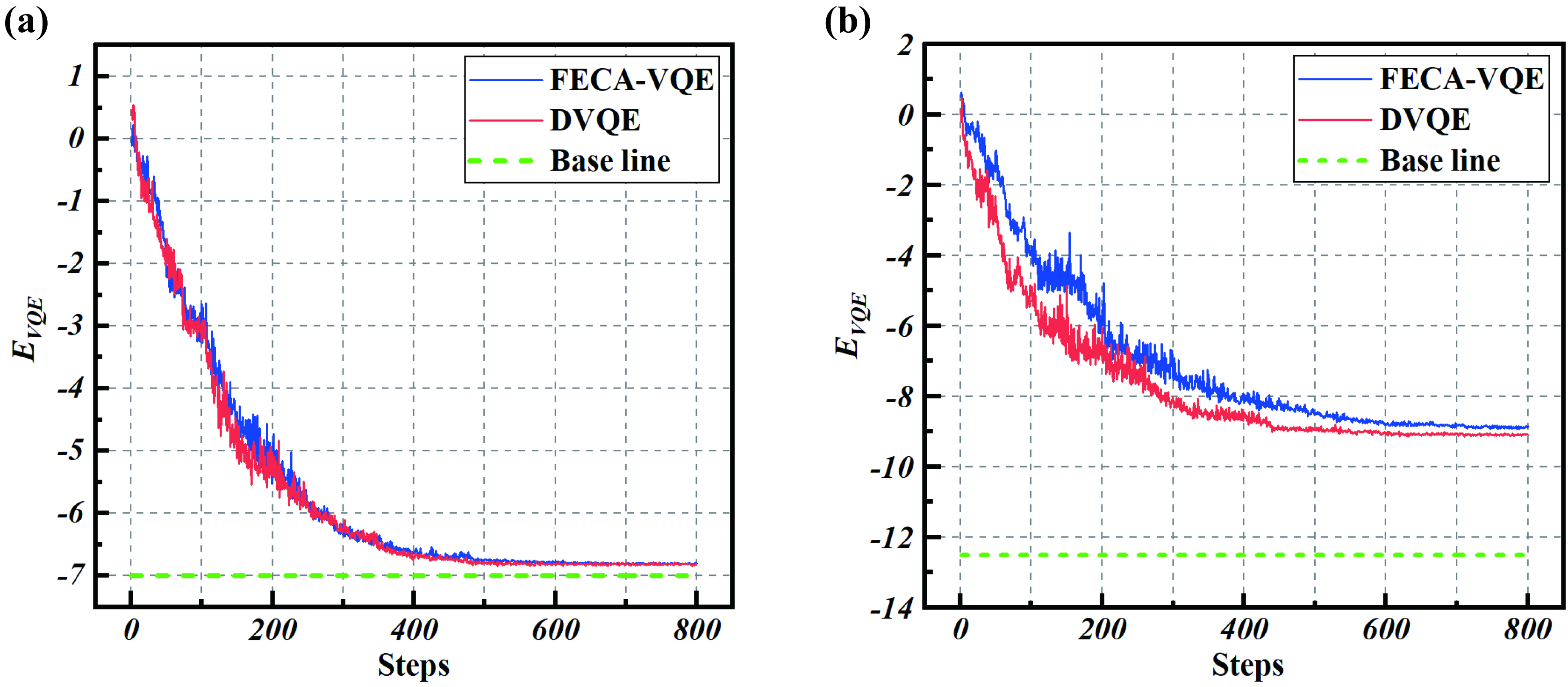
Figure 5: (a) & (b) The $E_{VQE}$ of both FECA-VQE and DVQE as a function of the training steps for the two-dimensional transverse-field Ising model and Heisenberg model, respectively. The size of the both models are $(2,3)$, and $L=5$. To obtain reliable results, we repeated each experiment five times then calculated the average.

Let’s first introduce the gate cutting technology briefly. Mitarai and Fuji proposed to construct a virtual two-qubit gate by sampling single-qubit operations, which can simulate effects of entanglement using classical post-processing and sampling [31]. In addition, it can also be used to simulate a large quantum circuit with small-scale quantum computers. According to their research, any two-qubit gate can be decomposed as follow:

$$\mathcal{S}(e^{i\theta{A_{1}\otimes{A_{2}}}})= cos^{2}\theta\mathcal{S}(I\otimes{I})+sin^{2}\theta\mathcal{S}(A_{1}\otimes{A_{2}})$$

$$+\frac{1}{8}cos\theta{sin\theta}\underset{(\alpha_{1},\alpha_{2})\in\{\pm 1\}^{2}}{\sum}\alpha_{1}\alpha_{2}[\mathcal{S}((I+\alpha_{1}A_{1})\otimes(I+i\alpha_{2}A_{2}))+\mathcal{S}((I+i\alpha_{1}A_{1})\otimes(I+\alpha_{2}A_{2}))],$$ (12)

where the $\mathcal{S}(U)$ is a superoperator definded by $\mathcal{S}(U)=U\rho{U^{\dagger}}$, i.e., a unitary operation $U$ onto a quantum state represented by density matrix $\rho$. The operations $\mathcal{S}(I+\alpha{A})$ and $\mathcal{S}(I+i\alpha{A})$ for $\alpha\in\{\pm 1\}$ can be implemented by projective measurement on the $A$ basis and single-qubit rotation about the $A$ axis for $A\in\{{X,Y,Z\}}$, respectively. The $CZ$ gate can be represented by

$$CZ=e^{i\pi{I\otimes{Z/4}}}e^{i\pi{Z\otimes{I/4}}}e^{-i\pi{Z\otimes{Z/4}}},$$ (13)

so we can decompose it into a sequence of single-qubit operations. To provide a clear illustration of the implementation details, we present the needed set of quantum sub-circuits for simulating the $CZ$ gate in Fig. 4.

By employing above gate cutting technology on the single entangling connection gate (e.g., the $CZ$ gate represented by the blue square in Fig. 1(c)), the SECA can be divided into multiple separate sub-circuits with just one cut. To validate the feasibility of the DVQE, we conduct simulation experiments with the two-dimensional Ising model as well as Heisenberg model and contrast the computational performance of DVQE with that of FECA-VQE. For relatively simple models like the two-dimensional Ising model, $E_{VQE}$ of both FECA-VQE and DVQE yield excellent approximations to the exact ground state energy, with similar rates of descent observed in the loss function, as shown in Fig. 5(a). For the more complex two-dimensional Heisenberg model, we observe a slight improvement in computational performance of the DVQE based on SECA compared to the FECA-VQE. This is manifested by a slightly faster descent rate and a slightly lower convergence value in $E_{VQE}$, as shown in the Fig. 5(b). Consequently, the aforementioned classical simulation experiments indicate that the DVQE based on SECA can not only effectively expand the size of NISQ device with a remarkably low overheads but also facilitate efficient execution of large-scale VQE tasks.

IV Discussion and conclusion

Considering the fact that near-term NISQ devices are difficult to meet the application requirements of quantum computing, such as the most promising example of VQE, we propose the single entanglement connection architecture (SECA) for the HEA-VQE and combine it with the gate cutting technology to construct distributed VQE (DVQE) which can efficiently expand the size of NISQ devices under low overheads. Our simulation experiments first confirm the superior computational performance of SECA-VQE over FECA-VQE and then prove the effectiveness and efficiency of DVQE scheme. The low overheads are reflected in the fact that only one gate cut is required for DVQE. The challenge of the application of gate cutting technology is that as the number of the gate cut increases, the overheads for implementing these gate cut grow exponentially. As shown in Fig. 4 each gate cut requires execution of 10 sub-circuits. The number of sub-circuits executed is $10^{L}$ for DVQE based on FECA which need $L$ gate cut. However, for DVQE based on SECA, only one gate cut is needed and the overheads can be reduced from $10^{L}$ to 10. While in this work we have only discussed the case of involving two multi-layer HEA, i.e., two QPUs, the DVQE scheme can be easily extended to the case of multiple QPUs. The corresponding overheads can be represented as $10^{N_{QPU}-1}$, where $N_{QPU}$ is the number of QPUs used in the DVQE scheme. Moreover, if we using mid-circuit measurement [33], each gate cut only requires execution of 6 sub-circuits, the overheads will fall further.

Based on these numerical experiments, we also find some interesting phenomenon which may be a useful hint or indication to engineer the hard problem about the relationship among entangling capacity, expressibility and computational performance. One of the phenomenon is that for SECA, as $L$ increases, both $Exp$ and $Ent$ reach a plateau. However, its computation performance still continues deteriorate. This implys that there are other characteristics of PQCs except for expressive power and entangling capability that may affect its computational performance. Another phenomenon is that the increase in $Exp$ is associated with the decrease in $Ent$. This is in line with our physical intuition that the reduction in $Ent$ would enhance the effectiveness of PQCs in exploring states with low entanglement, thereby advantageously impacting $Exp$. Additionally, some recent research show that both high expressive power and entangling capability can result in small variance in the cost gradient and hence the flat landscape [59, 61, 62, 63]. Thus, our better computational performance may be attributed to the balance between $Exp$ and $Ent$. However, this is just a numerical relation under certain condition. A more fundamental and general relationship should be drawn in the future research.