Propagation of generalized Korteweg-de Vries solitons along large-scale waves

Abstract

We consider propagation of solitons along large-scale background waves in the generalized Korteweg-de Vries (gKdV) equation theory when the width of the soliton is mach smaller than the characteristic size of the background wave. Due to this difference in scales, the soliton’s motion does not affect the dispersionless evolution of the background wave. We obtained the Hamilton equations for soliton’s motion and derived simple relationships which express the soliton’s velocity in terms of a local value of the background wave. Solitons’ paths obtained by integration of these relationships agree very well with the exact numerical solutions of the gKdV equation.

I Introduction

Perturbation theory for solitons has a long history and a number of publications is devoted to different approaches to it which span from simple variational estimates to rigorous mathematical investigations based on the inverse scattering transform method (see, e.g., review articles [1, 2] and references therein). In spite of that, there still exist some specific situations where the developed so far methods are either insufficient of too complicated for practical use and simpler approaches are needed. One such a situation refers to propagation of solitons along a large-scale background wave $u=\overline{u}(x,t)$, where $\overline{u}(x,t)$ obeys in the simplest case of unidirectional propagation to the Hopf-like equation

$$\overline{u}_{t}+V_{0}(\overline{u})\overline{u}_{x}=0.$$ (1)

If we denote a characteristic width of a soliton as $\sim\kappa^{-1}$, then it is assumed that $\overline{u}(x,t)$ changes considerably at distances about $l$ much greater than $\sim\kappa^{-1}$, so that $(\kappa l)^{-1}\ll 1$ is a small parameter of the theory. At the same time, Eq. (1) is just a dispersionless approximation of the nonlinear wave equation under consideration for unidirectional wave propagation. It is supposed that soliton’s propagation does not influence on evolution of the background wave, so this equation does not contain any perturbation terms. This scheme corresponds to the generally accepted qualitative picture according to which the soliton’s propagation through a non-uniform and varying with time background can be treated as motion of a classical particle under action of external time-dependent field. Consequently, the first task is to derive equations for soliton’s motion along the evolving background wave $u=\overline{u}(x,t)$. In fact, this problem was solved for Korteweg-de Vries (KdV) solitons in Refs. [3, 4] (see also [5, 6]), but this rigorous approach was quite involved mathematically and was not, apparently, widely used in physical literature. Recently this problem was reconsidered in Ref. [7] for propagation of KdV solitons along rarefaction waves by different methods including the Whitham theory of modulations, and this approach was extended to the problem of propagation of KdV solitons along dispersive shock waves (DSWs).

Application of the Whitham modulation theory to this type of problems seems very natural since propagation of the soliton edge of a DSW reduces exactly to the motion of the leading soliton along the background dispersionless wave. For example, this approach easily reproduces equations of motion [8] in Bose-Einstein condensate in case of absence of external perturbations (see Ref. [9]). In this paper we combine some ideas developed earlier in the Whitham modulation theory with elementary results of the perturbation theory and reproduce very simply the Hamilton equations of Refs. [3, 4] for soliton’s motion. These equations can be integrated to give a useful relationship

$$\kappa=\kappa(\overline{u})$$ (2)

between the soliton’s inverse half-width $\kappa$ and the background wave amplitude $\overline{u}$. Since soliton’s velocity $V$ can be expressed in terms of the dispersion relation $\omega=\omega(k,\overline{u})$ for linear waves with wave number $k$ propagating along the constant background $\overline{u}$ by the Stokes formula [10] (it was published first in the early edition of Lamb’s “Hydrodynamics”[11], section 252; see also [12] and references therein)

$$V=\frac{\omega(i\kappa,\overline{u})}{i\kappa},$$ (3)

then substitution of Eq. (2) gives the equation

$$\frac{dx}{dt}=V(\overline{u}(x,t))$$ (4)

for soliton’s path $x=x(t)$ which can be easily integrated.

The relationship (2) can be treated as an analytical continuation of the relationship between the carrier wave number $k$ of a short-wavelength wave packet and the background amplitude $\overline{u}$ which follows from the Hamilton theory of propagation of such packets [13] as well as from the Whitham theory for propagation of small-amplitude edges of dispersive shock waves [14]. This observation allows us to extend the theory to the generalized KdV equation and this is the main task of the present article. Our analytical results are confirmed by exact numerical solutions of particular problems of propagation of solitons along large-scale background waves.

II Motion of KdV soliton along a background wave

The KdV equation

$$u_{t}+6uu_{x}+u_{xxx}=0$$ (5)

describes evolution of the whole wave structure

$$u(x,t)=\overline{u}(x,t)+u_{s}(x,t)$$ (6)

which consists of the background large-scale wave $\overline{u}(x,t)$ obeying in our approximation to the Hopf equation

$$\overline{u}_{t}+6\overline{u}\,\overline{u}_{x}=0$$ (7)

and the soliton

$$u_{s}(x,t)=\frac{\kappa^{2}}{2}\cdot\frac{1}{\cosh^{2}[\kappa(x-x_{s}(t))/2]},$$ (8)

where $x_{s}(t)$ denotes the instant position of the soliton and $\kappa=\kappa(t)$ is its time-dependent inverse half-width.

Our first task is to derive the Hamilton equations for the particle-like motion of solitons. To this end, we notice that the dispersion relation for linear waves propagating along constant background $u=\overline{u}=\mathrm{const}$ reads

$$\omega(k,\overline{u})=6\overline{u}k-k^{3}.$$ (9)

Then, according to the Stokes rule (3), the soliton’s velocity is given by

$$\frac{dx}{dt}=\frac{\omega(i\kappa)}{i\kappa}=6\overline{u}(x,t)+\kappa^{2}=\frac{\partial H}{\partial p},$$ (10)

where we assume that the background $\overline{u}=\overline{u}(x,t)$ has the value corresponding to the position $x$ of the soliton at the instant $t$. We expressed this velocity in Eq. (10) in Hamiltonian form, where the Hamiltonian $H=H(x,p)$ and the canonical momentum $p$ are to be determined. The inverse half-width $\kappa$ must be some function of $p$. We write this dependence in the form $\kappa^{2}=f(p)$, so integration of Eq. (10) gives

$$H=6\overline{u}p+\int f(p)dp.$$ (11)

To find $f(p)$, we need one more equation and, following Ref. [7], we get it from the first non-trivial conservation law for solitons. Substitution of Eq. (6) into (5) gives

$$u_{s,t}+6(\overline{u}u_{s})_{x}+6u_{s}u_{s,x}+u_{s,xxx}=-F[\overline{u}(x,t)],$$ (12)

where

$$F[\overline{u}(x,t)]=\overline{u}_{t}+6\overline{u}\,\overline{u}_{x}+\overline{u}_{xxx}.$$ (13)

We assume that $\overline{u}(x,t)$ is a smooth solution of the Hopf equation (7), so the dispersion term in Eq. (13) can be neglected and we can take $F=0$. Then an easy calculation with the use of several integrations by parts yields

$$\begin{split}&\frac{d}{dt}\int_{-\infty}^{\infty}u_{s}^{2}dx=-12\int_{-\infty}^{\infty}u_{s}(\overline{u}u_{s})_{x}dx\\ &=-6\int_{-\infty}^{\infty}\overline{u}_{x}u_{s}^{2}dx\approx-6\overline{u}_{x}(x,t)\int_{-\infty}^{\infty}u_{s}^{2}dx,\end{split}$$ (14)

where we assume that since the distribution (8) has a form of a narrow peak, the smooth function $\overline{u}_{x}$ can be replaced with good enough accuracy by its value at the soliton’s position $x$ and the moment $t$. With the use of Eq. (8) we find at once that

$$\int_{-\infty}^{\infty}u_{s}^{2}dx=\frac{2}{3}\kappa^{3},$$ (15)

so Eq. (14) transforms to the needed equation

$$\frac{d\kappa^{2}}{dt}=-4\overline{u}_{x}\kappa^{2}.$$ (16)

Now, substitution of Eqs. (11) and (16) into the Hamilton equation

$$\frac{dp}{dt}=-\frac{\partial H}{\partial x}$$

gives with account of $p=p(f)=p(\kappa^{2})$

$$\frac{dp}{df}\cdot\frac{d\kappa^{2}}{dt}=-\frac{dp}{df}\cdot 4\overline{u}_{x}f=-\frac{\partial H}{\partial x}=-6\overline{u}_{x}p,$$

and, consequently, $2dp/p=3df/f$, so $p=f^{3/2}$ or $f=p^{2/3}$, where we have chosen the integration constant equal to unity for simplicity of the notation. At last, substitution of the function $f=p^{2/3}$ into Eq. (11) yields the Hamiltonian in the form

$$H=6\overline{u}(x,t)p+\frac{3}{5}p^{5/3}.$$ (17)

Soliton moves along the background wave $\overline{u}=\overline{u}(x,t)$ according to the Hamilton equations

$$\begin{split}&\frac{dx}{dt}=\frac{\partial H}{\partial p}=6\overline{u}(x,t)+p^{2/3},\\ &\frac{dp}{dt}=-\frac{\partial H}{\partial x}=-6\overline{u}_{x}(x,t)p.\end{split}$$ (18)

Equations (17), (18) coincide up to the notation with the equations obtained in Refs. [3, 4, 5] by a different method.

It is instructive to compare the above theory with the theory of Ref. [15] where it was shown that the KdV equation is a completely integrable Hamiltonian system in framework of the inverse scattering transform method discovered in Ref. [16]. The authors of Ref. [15] showed that the dynamics of any KdV wave reduces to the Hamiltonian dynamics of the “scattering data” for the associated Schrödinger spectral problem, where solitons correspond to the discrete part of the spectrum and the “background” to its continuous part. In this exact theory, one does not separate characteristic sizes of “narrow” solitons and “wide” background, so contributions of the background to the momentum and energy are given by quite complicated formulas relating them with the scattering amplitude. In our approximate approach the background dynamics is described by a simple dispersionless equation (7). At the same time, the both approaches lead to actually the same Hamiltonian dynamics for a single soliton propagating along a zero background. In particular, according to Refs. [15, 17] the expressions for the momentum and energy are given in terms of the inverse half-width $\kappa$ by the formulas

$$\widetilde{p}=\frac{1}{3}\kappa^{3},\quad\widetilde{H}=\frac{1}{5}\kappa^{5},\quad\text{so that}\quad\widetilde{H}=\frac{3^{1/3}}{5}p^{5/3},$$ (19)

which can be transformed to our formulas

$$p=\kappa^{3},\quad H=\frac{3}{5}\kappa^{5},\quad\text{so that}\quad H=\frac{3}{5}p^{5/3},$$ (20)

by multiplication of $\widetilde{p}$ and $\widetilde{H}$ by the constant factor 3 (obviously, the Hamilton equations are invariant with respect to this transformation). Then addition of the term $6\overline{u}p$ to this Hamiltonian can be interpreted as the Galileo transform of the energy due to motion of the background reference frame with velocity $6\overline{u}$.

We have arrived at the Hamiltonian system (18) which remains Hamiltonian when $\overline{u}(x,t)$ evolves according to the hydrodynamic equation (7). This means that the Poincaré-Cartan integral invariant [18, 19]

$$I(C)=\oint_{C}(p\delta x-H\delta t)$$ (21)

is preserved by the hydrodynamic flow (7). As was shown in Ref. [20], this implies that the momentum $p$ of the moving soliton depends on $x$ and $t$ only via the local value of the background variable $\overline{u}(x,t)$. To find this dependence, we define first a contour $C_{0}$ in the phase plane $(x,p)$ at $t=0$ and a tube of trajectories in the extended space $(x,p,t)$ stemming from the initial points of $C_{0}$ and generated by the flow $dx/dt=V_{0}(\overline{u}(x,t))$, where $\overline{u}(x,t)$ obeys Eq. (1). Next, we form an arbitrary contour $C$ around this tube by means of introduction of a coordinate $\mu$ along each trajectory and assume that $\mu$ is related with $x$ and $t$ by the equations

$$\frac{dx}{V_{0}(\overline{u})}=dt=\chi(t,x,p(\overline{u}))d\mu,$$

where $\chi$ is an arbitrary function, so that the contour $C$ depends on the choice of $\chi$ and on the value of $\mu$. At last, we demand that $I$ does not depend on $\mu$, that is $dI/dt=0$, then an easy calculation yields the condition

$$\oint_{C}\left[\left(\frac{\partial H}{\partial p}-V_{0}\right)\frac{dp}{d\overline{u}}+\frac{\partial H}{\partial\overline{u}}\right]\chi\left(\frac{\partial\overline{u}}{\partial t}\delta t+\frac{\partial\overline{u}}{\partial x}\delta x\right)=0.$$

Consequently, in view of arbitrariness of the function $\chi$, we arrive at the equation for the function $p=p(\overline{u})$,

$$\frac{dp}{d\overline{u}}=\frac{\partial H/\partial\overline{u}}{V_{0}(\overline{u})-\partial H/\partial p}.$$ (22)

In our case with $V_{0}=6\overline{u}$ and $H$ defined by Eq. (17), this equation takes the form $p^{-1/3}dp=-6d\overline{u}$, so we get

$$p^{2/3}=-4\overline{u}(x,t)+q,$$ (23)

where $q$ is an integration constant. According to our definitions above, $p^{2/3}=f=\kappa^{2}$, so this relation can be written as

$$\kappa^{2}=-4\overline{u}(x,t)+q.$$ (24)

At last, substitution of Eq. (23) into the first Hamilton equation (18) gives a very simple equation for the soliton’s path

$$\frac{dx}{dt}=2\overline{u}(x,t)+q,$$ (25)

where it is assumed that $\overline{u}(x,t)$ is a known solution of Eq. (7) and $q$ is determined by the initial soliton’s velocity. It is worth noticing that Eq. (22) transformed from $p$ to the variable $\kappa=p^{1/3}$ coincides with the equation introduced by G. A. El in Ref. [14] for description of motion of the soliton edge of dispersive shock waves generated from evolution of step-like initial discontinuities.

Eq. (24) can be obtained in a simpler way with help of the Stokes reasoning [10, 11] based on observation that the exponentially small soliton tails $u_{s}\propto\exp[\pm\kappa(x-V_{s}t)]$ and the small-amplitude harmonic waves $\propto\exp[i(kx-\omega t)]$ obey the same linearized equations, so the transformation $k\mapsto i\kappa$ converts the phase velocity $V(k)=\omega(k)/k$ into the soliton’s velocity (3). From this point of view, the formula (3) for the soliton velocity is just an analytical continuation of the formula $V(k)=\omega(k)/k$ for the phase velocity from the real $k$-axis to its imaginary axis in the complex $k$-plane. This idea of analytical continuation can be applied to some other expressions obtained for motion of high-frequency wave packets converting them to relations between the soliton’s parameters (see Ref. [20]). For example, motion of a localized wave packet is described by its coordinate $x=x(t)$ and carrier wave number $k=k(t)$ which obey the Hamilton equations

$$\frac{dx}{dt}=\frac{\partial\omega}{\partial k},\qquad\frac{dk}{dt}=-\frac{\partial\omega}{\partial x}.$$ (26)

Again, when such a packet propagates along a background wave which evolves according to Eq. (7), the wave number $k$ is a function of $\overline{u}$ determined by the equation [14, 13]

$$\frac{dk}{d\overline{u}}=\frac{\partial\omega/\partial\overline{u}}{V_{0}(\overline{u})-\partial\omega/\partial k},$$ (27)

which in the KdV equation case (7) and (9) gives at once

$$k^{2}=4\overline{u}-q,$$ (28)

where $q$ is an integration constant. Analytical continuation of this formula to soliton’s region according to the Stokes rule $k\mapsto i\kappa$ reproduces Eq. (24). The advantage of this method, based on the well-established asymptotic theory of propagation of high-frequency wave packets, is that it does not need derivation of Eqs. (18) or (22). At last we notice that formulas (24) and (28) also follow from the Whitham modulation equations [21, 22] at their soliton and small-amplitude edges, correspondingly.

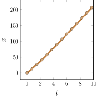
(a)

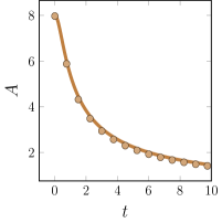
(b)

Figure 1: (a) Soliton’s path $x(t)$ obtained from solution of Eq. (31) (solid line) and from exact numerical solution of the KdV equation (5). (b) Change of the soliton’s amplitude $A$ during propagation of the soliton along the background wave (30); solid line corresponds to Eq. (32) and dots to the numerical solution of the KdV equation.

Let us illustrate this theory by an example of propagation of a KdV soliton with the initial value $\kappa=4$, that is the initial amplitude $A=\kappa^{2}/2=8$, which starts its motion at the point $x=0$ at the moment $t=0$. The background wave has the initial profile

$$\overline{u}(x,0)=(x/8)^{2},\qquad x>0.$$ (29)

Then we obtain from Eq. (7) the profile

$$\overline{u}(x,t)=\frac{4}{9t^{2}}\left(\sqrt{1+\frac{3}{8}xt}-1\right)^{2},\qquad x>0,$$ (30)

at any moment of time $t\geq 0$. Since the initial velocity equals to $q=\kappa^{2}=16$, Eq. (25) takes the form

$$\frac{dx}{dt}=\frac{8}{9t^{2}}\left(\sqrt{1+\frac{3}{8}xt}-1\right)^{2}+16$$ (31)

and it should be solved with the initial condition $x(0)=0$. The plot of this solution is shown in Fig. 1(a) by a solid line and dots correspond to soliton’s positions obtained from numerical solution of the whole KdV equation (5) with the initial profile composed of the background wave (29) and the soliton (8) located at $x=0$ with $\kappa=4$. The solid line in Fig. 1(b) shows the analytical dependence (see Eq. (24))

$$A=\frac{\kappa^{2}}{2}=8-2\overline{u}(x(t),t)$$ (32)

of the soliton’s amplitude on time $t$ and dots correspond again to numerical values of the amplitude. As we see, our approximate analytical theory agrees very well with the exact numerical solution.

III Generalized KdV equation

Here we shall apply the above approach to the generalized KdV (gKdV) equation

$$u_{t}+V_{0}(u)u_{x}+u_{xxx}=0,$$ (33)

where $V_{0}(u)$ is a monotonously growing function of $u$, $V_{0}(0)=0$. If we look for a soliton solution in the form $u=u(\xi)$, $\xi=x-Vt$, when it propagates along a constant background $u\to\overline{u}$ as $|\xi|\to\infty$, then an easy calculation lead to the equation

$$\begin{split}u_{\xi}^{2}=G(u),\quad G(u)=&V(u-\overline{u})^{2}-2\left[\Phi(u)-\Phi(\overline{u})\right]\\ &+2\Phi^{\prime}(\overline{u})(u-\overline{u}),\end{split}$$ (34)

where

$$\Phi(u)=\int_{0}^{u}du^{\prime}\int_{0}^{u^{\prime}}V_{0}(u^{\prime\prime})du^{\prime\prime}.$$ (35)

The expression in the right-hand side of Eq. (34) has a double zero at $u=\overline{u}$. One more zero $u=u_{m}>\overline{u}$ defines the soliton’s amplitude by the equation

$$\frac{1}{2}V(u_{m}-\overline{u})^{2}=\left[\Phi(u_{m})-\Phi(\overline{u})\right]-\Phi^{\prime}(\overline{u})(u_{m}-\overline{u}),$$ (36)

so that

$$A=u_{m}-\overline{u}.$$ (37)

The soliton’s profile is determined in implicit form by the quadrature

$$\xi=\int_{u}^{u_{m}}\frac{du}{\sqrt{G(u)}}.$$ (38)

We assume that this solution is stable. For example, in case of

$$V_{0}(u)=6u^{\gamma}$$ (39)

the soliton solution is stable, if $0<\gamma<4$ (see Ref. [23]). In a particular case of modified KdV (mKdV) equation with $\gamma=2$ the soliton solution can be written in explicit form

$$u(\xi)=\overline{u}+\frac{V-6\overline{u}^{2}}{\sqrt{V-2\overline{u}^{2}}\cosh(\sqrt{V-6\overline{u}^{2}}\xi)+2\overline{u}}.$$ (40)

Consequently, in this case the inverse half-width $\kappa$ is related with the soliton’s velocity $V$ by the formula

$$\kappa^{2}=V-6\overline{u}^{2}$$ (41)

and the amplitude is equal to

$$A=\frac{V-6\overline{u}^{2}}{\sqrt{V-2\overline{u}^{2}}+2\overline{u}}.$$ (42)

Now we turn to the problem of propagation of solitons along smooth large scale background waves. In case of the gKdV equation (33) we get the dispersion relation for harmonic waves

$$\omega(k,\overline{u})=V_{0}(\overline{u})k-k^{3}.$$ (43)

It is assumed that the wavelength is much smaller than a characteristic size of the background wave $\overline{u}$ whose evolution is described by Eq. (1). Now Eq. (27) gives (see [14, 12])

$$k^{2}=\frac{2}{3}V_{0}(\overline{u})-q,$$ (44)

$q$ is an integration constant. Analytical continuation of this formula to the soliton region yields the expression for the soliton’s inverse half-width

$$\kappa^{2}=q-\frac{2}{3}V_{0}(\overline{u}).$$ (45)

Consequently, the Stokes rule (3) gives the expression for the soliton’s velocity

$$\frac{dx}{dt}=V=\frac{\omega(i\kappa,\overline{u})}{i\kappa}=V_{0}(\overline{u})+\kappa^{2}=\frac{1}{3}V_{0}(\overline{u})+q,$$ (46)

where the integration constant $q$ is determined by the initial conditions. Integration of this equation with known law $\overline{u}=\overline{u}(x,t)$ of evolution of the background wave gives the path $x=x(t)$ of the soliton. In case of the mKdV equation we get

$$\frac{dx}{dt}=V=2\overline{u}^{2}(x,t)+q$$ (47)

and substitution of this expression for $V$ to Eq. (42) gives the dependence of the amplitude along the soliton’s path,

$$A(t)=\sqrt{q}-2\overline{u}(x(t),t).$$ (48)

Of course, this result can also be obtained directly from Eq. (36), which is applicable to the general nonlinearity function $V_{0}(u)$, with the use of Eqs. (37) and (46).

The Hamilton equations for soliton’s motion in case of the gKdV equation can be obtained without much difficulty. We denote again $\kappa^{2}=f(p)$ and integration of the equation

$$\frac{dx}{dt}=\frac{\partial H}{\partial p}=V=V_{0}(\overline{u})+\kappa^{2}=V_{0}(\overline{u})+f(p)$$

gives

$$H=V_{0}(\overline{u})p+\int f(p)dp.$$ (49)

Differentiation of Eq. (45) along the soliton’s path yields

$$\frac{d\kappa^{2}}{dt}=-\frac{2}{3}V_{0}^{\prime}(\overline{u})(\overline{u}_{t}+V\overline{u}_{x})=-\frac{2}{3}V_{0}^{\prime}(\overline{u})\overline{u}_{x}\kappa^{2}.$$

Then the second Hamilton equation $dp/dt=-\partial H/\partial x$ gives

$$\frac{dp}{df}\cdot\left(-\frac{2}{3}V_{0}^{\prime}(\overline{u})\overline{u}_{x}f\right)=-V_{0}^{\prime}(\overline{u})\overline{u}_{x}p$$

and, hence, $f(p)=p^{2/3}$, $p=\kappa^{3}$. Thus, we obtain the Hamiltonian

$$H=V_{0}(\overline{u}(x,t))p+\frac{3}{5}p^{5/3}$$ (50)

and the Hamilton equations

$$\frac{dp}{dt}=-V_{0}^{\prime}(\overline{u})\overline{u}_{x}p,\qquad\frac{dx}{dt}=V_{0}(\overline{u})+p^{2/3}.$$ (51)

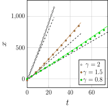
Figure 2: Paths $x(t)$ of the solitons propagating along the background waves (53) for different data sets ($\gamma,a,v_{0},x_{0}$): gray ($2,0.25,40,-20$), brown ($1.5,0.1,15,-25$) and green ($0.8,0.005,10,0$). The circles correspond to the numerical solution of Eq.(33), the solid lines to Eq. (55), and the dashed lines correspond to free motion of the soliton along a zero background.

Let us apply the developed theory to the problem of propagation of solitons in case of the nonlinearity function (39) and for the initial background wave distribution

$$\overline{u}_{0}(x)=\left\{\begin{array}[]{ll}a(x/5)^{1/\gamma},&x>0,\\ 0,&x<0.\end{array}\right.$$ (52)

Then the solution of the Hopf equation (1) reads

$$\overline{u}(x,t)=a\left(\frac{x}{t/\tau+5}\right)^{1/\gamma},\quad\tau=\frac{1}{6a^{\gamma}},$$ (53)

and $V_{0}(\overline{u})$ is given by

$$V_{0}(\overline{u}(x,t))=\frac{x}{t+5\tau}.$$ (54)

Let the soliton start its motion at the point $x=0$ at the moment $t=t_{0}>0$ with the initial velocity $v_{0}$. Then Eq. (46) takes the form

$$\frac{dx}{dt}=\frac{1}{3}\frac{x}{t+5\tau}+v_{0}$$ (55)

and it can be easily solved to give

$$x(t)=\frac{3}{2}v_{0}(t+5\tau)\left\{1-\left(\frac{t_{0}+5\tau}{t+5\tau}\right)^{2/3}\right\}.$$ (56)

The soliton’s amplitude along the path can be found from Eqs. (36), (37) with

$$\Phi(\overline{u})=\frac{6}{(\gamma+1)(\gamma+2)}\overline{u}^{\gamma+2}$$ (57)

and $V$ is defined by Eq. (55). These analytical predictions are compared with numerical solutions of Eq. (33) in Fig. 2 and very good agreement is observed.

IV Conclusion

We showed that the KdV soliton dynamics along a large-scale background wave can be reduced to Hamilton equations with the use of elementary perturbation theory argumentation. Preservation of the Hamiltonian structure by the dispersionless flow leads to a simple relationship between the inverse half-width of a moving soliton and a local value of the background wave. This relationship can be interpreted as an analytical continuation of the relationship between the carrier wave number of a wave packet propagating along a large-scale background wave which follows from the well-known optical-mechanical analogy where the packet’s dynamics is also treated by the Hamilton methods. This type of reasoning first introduced by Stokes allows one to extend the theory to the generalized KdV equation case and the analytical results are confirmed by comparison with exact numerical solutions.

We believe that our approach based on preservation of Hamiltonian dynamics of both high-frequency wave packets and narrow solitons by dispersionless hydrodynamic flow can be applied to other problems of soliton dynamics.

- [1] B. A. Malomed, Variational methods in nonlinear fiber optics and related fields, in Progress in Optics, ed. E. Wolf, vol. 43, p. 69, (Elsevier, Amsterdam, 2002).
- [2] Y. S. Kivshar and B. A. Malomed, Dynamics of solitons in nearly integrable systems, Rev. Mod. Phys., 61, 763 (1989).
- [3] V. P. Maslov and V. A. Tsupin, Nessesary conditions for the existence of infinetely narrow solitons in gas dynamics (Russian) Dokl. Akad. Nauk SSSR, 246, 298 (1979) [Soviet Phys. Dokl., 24, 354 (1979)].
- [4] V. P. Maslov and G. A. Omel´yanov, Asymptotic soliton-form solutions of equations with small dispersion, Uspekhi Mat. Nauk., 36, No. 3, 63 (1981) [Russian Math. Surveys, 36, No. 3, 73 (1981)].
- [5] V. P. Maslov and G. A. Omel´yanov, Geometric Asymptotics for Nonlinear PDE. I, (AMS, Providence, 2001).
- [6] I. A. Molotkov, Analytical Methods in Nonlinear Wave Theory, (Pensoft Publishers, Sofia-Moscow, 2005).
- [7] M. J. Ablowitz, J. T. Cole, G. A. El, M. A. Hoefer, and X.-D. Luo, Soliton-mean field interaction in Korteweg-de Vries dispersive hydrodynamics, Stud. Appl. Math. (2023); DOI: 10.1111/sapm.12615; preprint arXiv:2211.14884 (2022).
- [8] Th. Busch, J. R. Anglin, Motion of dark solitons in trapped Bose-Einstein condensates, Phys. Rev. Lett. 84, 2298-2301 (2000).
- [9] S. K. Ivanov and A. M. Kamchatnov, Motion of dark solitons in a non-uniform flow of Bose-Einstein condensate, Chaos 32, 113142 (2022).
- [10] G. G. Stokes, Mathematical and Physical Papers, Vol. V, p. 162 (Cambridge University Press, Cambridge, 1905).
- [11] H. Lamb, Hydrodynamics, (Cambridge University Press, Cambridge, 1932).
- [12] A. M. Kamchatnov, Theory of quasi-simple dispersive shock waves and number of solitons evolved from a nonlinear pulse, Chaos, 30, 123148 (2020).
- [13] A. M. Kamchatnov and D. V. Shaykin, Propagation of wave packets along intensive simple waves, Phys. Fluids, 33, 052120 (2021).
- [14] G. A. El, Resolution of a shock in hyperbolic systems modified by weak dispersion, Chaos, 15, 037103 (2005).
- [15] V. E. Zakharov, L. D. Faddeev, Korteweg-de Vries equation: A completely integrable Hamiltonian system, Funk. Analiz Prilozh., 5, 18 (1971)[Func. Anal. Appl., 5, 280 (1971)].
- [16] C. S. Gardner, J. M. Greene, M. D. Kruskal, and R. M. Miura, Method for solving the Korteweg-de Vries equation, Phys. Rev. Lett., 19, 1095 (1967).
- [17] V. E. Zakharov, S. V. Manakov, S. P. Novikov, and L. P. Pitaevskii, The Theory of Solitons: The Inverse Scattering Method, (Nauka, Moscow, 1980) (translation: Consultants Bureau, 1984).
- [18] H. Poincaré, Les méthodes nouvelles de la Mécanique céleste, t. III, (Paris, Gauthier-Villar, 1899).
- [19] É. Cartan, Leçons sur les invariants intégraux, (Hermann, Paris, 1922).
- [20] A. M. Kamchatnov, Asymptotic theory of not completely integrable soliton equations, Chaos, 33, 093105 (2023).
- [21] G. B. Whitham, Non-linear dispersive waves, Proc. Roy. Soc. London, A 283, 238 (1965).
- [22] G. B. Whitham, Linear and Nonlinear Waves, (Wiley Interscience, New York, 1974).
- [23] E. A. Kuznetsov, Soliton stability in equations of the KdV type, Phys. Lett. A 101, 314 (1984).