ASCON: Anatomy-aware Supervised Contrastive Learning Framework for Low-dose CT Denoising

Abstract

While various deep learning methods have been proposed for low-dose computed tomography (CT) denoising, most of them leverage the normal-dose CT images as the ground-truth to supervise the denoising process. These methods typically ignore the inherent correlation within a single CT image, especially the anatomical semantics of human tissues, and lack the interpretability on the denoising process. In this paper, we propose a novel Anatomy-aware Supervised CONtrastive learning framework, termed ASCON, which can explore the anatomical semantics for low-dose CT denoising while providing anatomical interpretability. The proposed ASCON consists of two novel designs: an efficient self-attention-based U-Net (ESAU-Net) and a multi-scale anatomical contrastive network (MAC-Net). First, to better capture global-local interactions and adapt to the high-resolution input, an efficient ESAU-Net is introduced by using a channel-wise self-attention mechanism. Second, MAC-Net incorporates a patch-wise non-contrastive module to capture inherent anatomical information and a pixel-wise contrastive module to maintain intrinsic anatomical consistency. Extensive experimental results on two public low-dose CT denoising datasets demonstrate superior performance of ASCON over state-of-the-art models. Remarkably, our ASCON provides anatomical interpretability for low-dose CT denoising for the first time. Source code is available at https://github.com/hao1635/ASCON.

1 Introdcution

With the success of deep learning in the field of computer vision and image processing, many deep learning-based methods have been proposed and achieved promising results in low-dose CT (LDCT) denoising [1, 12, 23, 24, 26, 9, 6, 5, 4]. Typically, they employ a supervised learning setting, which involves a set of image pairs, LDCT images and their normal-dose CT (NDCT) counterparts. These methods typically use a pixel-level loss (e.g. mean squared error or MSE), which can cause over-smoothing problems.

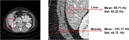
Figure S1: The mean and standard deviation of different tissues in an example of an LDCT image. The standard deviation (std) of an ROI in the liver is 63.23 HU, while the std of an ROI in the muscle is 44.73 HU.

To address this issue, a few studies [23, 26] used a structural similarity (SSIM) loss or a perceptual loss [11]. However, they all perform in a sample-to-sample manner and ignore the inherent anatomical semantics, which could blur details in areas with low noise levels. Previous studies have shown that the level of noise in CT images varies depending on the type of tissues [17]; see an example in Fig. S1 in Supplementary Materials. Therefore, it is crucial to characterize the anatomical semantics for effectively denoising diverse tissues.

In this paper, we focus on taking advantage of the inherent anatomical semantics in LDCT denoising from a contrastive learning perspective [7, 27, 25]. To this end, we propose a novel Anatomy-aware Supervised CONtrastive learning framework (ASCON), which consists of two novel designs: an efficient self-attention-based U-Net (ESAU-Net) and a multi-scale anatomical contrastive network (MAC-Net). First, to ensure that MAC-Net can effectively extract anatomical information, diverse global-local contexts and a larger input size are necessary. However, operations on full-size CT images with self-attention are computationally unachievable due to potential GPU memory limitations [20]. To address this limitation, we propose an ESAU-Net that utilizes a channel-wise self-attention mechanism [22, 28, 2] which can efficiently capture both local and global contexts by computing cross-covariance across feature channels.

Second, to exploit inherent anatomical semantics, we present the MAC-Net that employs a disentangled U-shaped architecture [25] to produce global and local representations. Globally, a patch-wise non-contrastive module is designed to select neighboring patches with similar semantic context as positive samples and align the same patches selected in denoised CT and NDCT which share the same anatomical information, using an optimization method similar to the BYOL method [7]. This is motivated by the prior knowledge that adjacent patches often share common semantic contexts [27]. Locally, to further improve the anatomical consistency between denoised CT and NDCT, we introduce a pixel-wise contrastive module with a hard negative sampling strategy [21], which randomly selects negative samples from the pixels with high similarity around the positive sample within a certain distance. Then we use a local InfoNCE loss [18] to pull the positive pairs and push the negative pairs.

Our contributions are summarized as follows. 1) We propose a novel ASCON framework to explore inherent anatomical information in LDCT denoising, which is important to provide interpretability for LDCT denoising. 2) To better explore anatomical semantics in MAC-Net, we design an ESAU-Net, which utilizes a channel-wise self-attention mechanism to capture both local and global contexts. 3) We propose a MAC-Net that employs a disentangled U-shaped architecture and incorporates both global non-contrastive and local contrastive modules. This enables the exploitation of inherent anatomical semantics at the patch level, as well as improving anatomical consistency at the pixel level. 4) Extensive experimental results demonstrate that our ASCON outperforms other state-of-the-art methods, and provides anatomical interpretability for LDCT denoising.

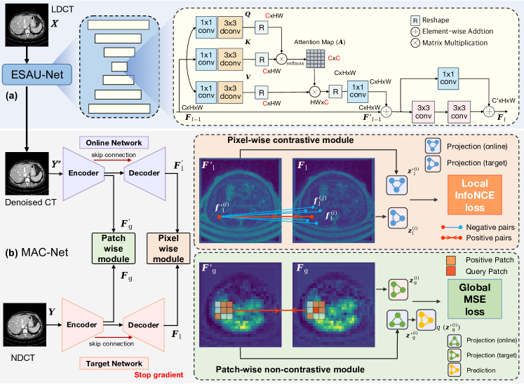
Figure 1: Overview of our proposed ASCON. (a) Efficient self-attention-based U-Net (ESAU-Net); and (b) multi-scale anatomical contrastive network (MAC-Net).

2 Methodology

2.1 Overview of the proposed ASCON

Fig. 1 presents the overview of the proposed ASCON, which consists of two novel components: ESAU-Net and MAC-Net. First, given an LDCT image, $\bm{X}\in\mathbb{R}^{1\times H\times W}$, where $H\times W$ denotes the image size. $\bm{X}$ is passed through the ESAU-Net to capture both global and local contexts using a channel-wise self-attention mechanism and obtain a denoised CT image $\bm{Y}^{\prime}\in\mathbb{R}^{1\times H\times W}$.

Then, to explore inherent anatomical semantics and remain inherent anatomical consistency, the denoised CT $\bm{Y}^{\prime}$ and NDCT $\bm{Y}$ are passed to the MAC-Net to compute a global MSE loss $\mathcal{L}_{\mathrm{{global}}}$ in a patch-wise non-contrastive module and a local infoNCE loss $\mathcal{L}_{\mathrm{{local}}}$ in a pixel-wise contrastive module. During training, we use an alternate learning strategy to optimize ESAU-Net and MAC-Net separately, which is similar to GAN-based methods [10]. Please refer to Alg. 1 in Supplementary Materials for a detailed optimization.

2.2 Efficient Self-attention-based U-Net

To better leverage anatomical semantic information in MAC-Net and adapt to the high-resolution input, we design the ESAU-Net that can capture both local and global contexts during denoising. Different from previous works that only use self-attention in the coarsest level [20], we incorporate a channel-wise self-attention mechanism [2, 28] at each up-sampling and down-sampling level in the U-Net [22] and add an identity mapping in each level, as shown in Fig. 1(a).

Specifically, in each level, given the feature map $\bm{F}_{l-1}$ as the input, we first apply a $1\times 1$ convolution and a $3\times 3$ depth-wise convolution to aggregate channel-wise contents and generate query ($\bm{Q}$), key ($\bm{K}$), and value ($\bm{V}$) followed by a reshape operation, where $\bm{Q}\in\mathbb{R}^{C\times HW}$, $\bm{K}\in\mathbb{R}^{C\times HW}$, and $\bm{V}\in\mathbb{R}^{C\times HW}$ (see Fig. 1(a)). Then, a channel-wise attention map $\bm{A}\in\mathbb{R}^{C\times C}$ is generated through a dot-product operation by the reshaped query and key, which is more efficient than the regular attention map of size ${HW\times HW}$ [3], especially for high-resolution input. Overall, the process is defined as

$$\tiny\operatorname{Attention}(\bm{F}) =w(\bm{V}^{T}\bm{A})=w(\bm{V}^{T}\cdot\operatorname{Softmax}({\bm{K}\bm{Q}^{T}}/{\alpha})),$$ (1)

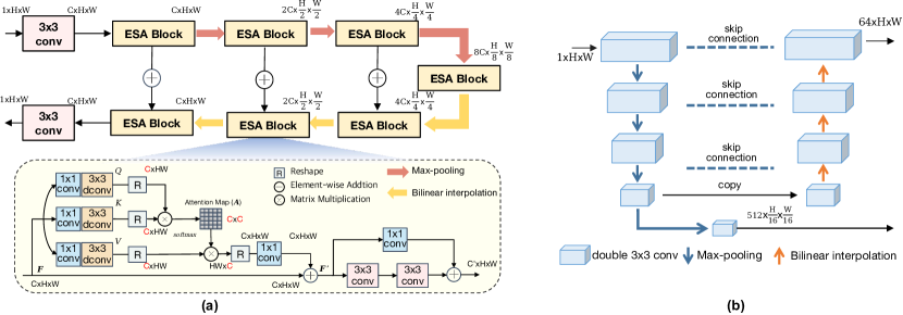
Figure S2: Overview of (a) ESAU-Net and (b) disentangled U-shape architecture.

where $w(\cdot)$ first reshapes the matrix back to the original size $C\times H\times W$ and then performs $1\times 1$ convolution; $\alpha$ is a learnable parameter to scale the magnitude of the dot product of $\bm{K}$ and $\bm{Q}$. We use multi-head attention similar to the standard multi-head self-attention mechanism [3]. The output of the channel-wise self-attention is represented as: ${\bm{F}^{\prime}_{l-1}}=\operatorname{Attention}(\bm{F}_{l-1})+\bm{F}_{l-1}$. Finally, the output $\bm{F}_{l}$ of each level is defined as: $\bm{F}_{l}=\operatorname{Conv}(\bm{F}^{\prime}_{l-1})+\operatorname{Iden}(\bm{F}_{l-1})$, where $\operatorname{Conv}(\cdot)$ is a two-layer convolution and $\operatorname{Iden}(\cdot)$ is an identity mapping using a $1\times 1$ convolution; refer to Fig. S2(a) for the details of ESAU-Net.

2.3 Multi-scale Anatomical Contrastive Network

Overview of MAC-Net. The goal of our MAC-Net is to exploit anatomical semantics and maintain anatomical embedding consistency, First, a disentangled U-shaped architecture [22] is utilized to learn global representation $\bm{F}_{\mathrm{g}}$ $\in\mathbb{R}^{512\times\frac{H}{16}\times\frac{W}{16}}$ after four down-sampling layers, and learn local representation $\bm{F}_{\mathrm{l}}$$\in\mathbb{R}^{64\times H\times W}$ by removing the last output layer. And we cut the connection between the coarsest feature and its upper level to make $\bm{F}_{\mathrm{g}}$ and $\bm{F}_{\mathrm{l}}$ more independent [25] (see Fig. S2(b)). The online network and the target network, both using the same architecture above, handle denoised CT $\bm{Y}^{\prime}$ and NDCT $\bm{Y}$, respectively, with $\bm{F}^{\prime}_{\mathrm{g}}$ and $\bm{F}^{\prime}_{\mathrm{l}}$ generated by the online network, and $\bm{F}_{\mathrm{g}}$ and $\bm{F}_{\mathrm{l}}$ generated by the target network (see Fig. 1(b)). The parameters of the target network are an exponential moving average of the parameters in the online network, following the previous works [8, 7]. Next, a patch-wise non-contrastive module uses $\bm{F}_{\mathrm{g}}$ and $\bm{F}^{\prime}_{\mathrm{g}}$ to compute a global MSE loss $\mathcal{L}_{\mathrm{global}}$, while a pixel-wise contrastive module uses $\bm{F}_{\mathrm{l}}$ and $\bm{F}^{\prime}_{\mathrm{l}}$ to compute a local infoNCE loss $\mathcal{L}_{\mathrm{local}}$. Let us describe these two loss functions specifically.

Patch-wise non-contrastive module. To better learn anatomical representations, we introduce a patch-wise non-contrastive module, also shown in Fig. 1(b). Specifically, for each pixel ${{\bm{f}}_{\mathrm{g}}^{(i)}}\in\mathbb{R}^{512}$ in the ${\bm{F}}_{\mathrm{g}}$ where $i\in\{1,2,\ldots,\frac{HW}{256}\}$ is the index of the pixel location, it can be considered as a patch due to the expanded receptive field achieved through a sequence of convolutions and down-sampling operations [19]. To identify positive patch indices, we adopt a neighboring positive matching strategy [27], assuming that a semantically similar patch ${{\bm{f}}_{\mathrm{g}}^{(j)}}$ exists in the vicinity of the query patch ${{\bm{f}}_{\mathrm{g}}^{(i)}}$, as neighboring patches often share a semantic context with the query. We empirically consider a set of 8 neighboring patches. To sample patches with similar semantics around the query patch ${{\bm{f}}_{\mathrm{g}}^{(i)}}$, we measure the semantic closeness between the query patch ${{\bm{f}}_{\mathrm{g}}^{(i)}}$ and its neighboring patches ${{\bm{f}}_{\mathrm{g}}^{(j)}}$ using the cosine similarity, which is formulated as

$$\small s(i,j)=({{\bm{f}}_{\mathrm{g}}^{(i)}})^{\top}({{\bm{f}}_{\mathrm{g}}^{(j)}})/\|{{\bm{f}}_{\mathrm{g}}^{(i)}}\|_{2}\|{{\bm{f}}_{\mathrm{g}}^{(j)}}\|_{2}.$$ (2)

We then select the top-4 positive patches $\{{{\bm{f}}_{\mathrm{g}}^{(j)}}\}_{j\in\mathcal{P}^{(i)}}$ based on $s(i,j)$, where $\mathcal{P}^{(i)}$ is a set of selected patches (i.e., $|\mathcal{P}^{(i)}|=4$). To obtain patch-level features $\bm{{g}}^{(i)}\in\mathbb{R}^{512}$ for each patch ${{\bm{f}}_{\mathrm{g}}^{(i)}}$ and its positive neighbors, we aggregate their features using global average pooling (GAP) in the patch dimension. For the local representation of ${{\bm{f}^{\prime}}_{\mathrm{g}}^{(i)}}$, we select positive patches as same as $\mathcal{P}^{(i)}$, i.e., $\{{{\bm{f}^{\prime}}_{\mathrm{g}}^{(j)}}\}_{j\in\mathcal{P}^{(i)}}$. Formally,

$$\small\bm{g}^{(i)}:=\operatorname{GAP}({{\bm{f}}_{\mathrm{g}}^{(i)}},\{{{{\bm{f}}_{\mathrm{g}}^{(j)}}\}_{j\in\mathcal{P}^{(i)}}}),\quad{{\bm{{g}}^{\prime}}^{(i)}}:=\operatorname{GAP}({{\bm{f}^{\prime}}_{\mathrm{g}}^{(i)}},\{{{{\bm{f}^{\prime}}_{\mathrm{g}}^{(j)}}\}_{j\in\mathcal{P}^{(i)}}}).$$ (3)

From the patch-level features, the online network outputs a projection ${{\bm{z}_{\mathrm{g}}^{\prime}}^{(i)}}={{p^{\prime}_{\mathrm{g}}}({{\bm{g}^{\prime}}^{(i)})}}$ and a prediction ${q^{\prime}}{({\bm{z}_{\mathrm{g}}^{\prime}}^{(i)})}$ while target network outputs the target projection ${\bm{z}_{\mathrm{g}}}^{(i)}={{p_{\mathrm{g}}}({{\bm{g}}^{(i)})}}$. The projection and prediction are both multi-layer perceptron (MLP). Finally, we compute the global MSE loss between the normalized prediction and target projection [7],

$$\mathcal{L}_{\mathrm{global}}=\sum\nolimits_{i\in{\mathcal{N}_{\mathrm{pos}}^{\mathrm{g}}}}\big{\|}{q^{\prime}}({\bm{z}_{\mathrm{g}}^{\prime}}^{(i)})-{\bm{z}_{\mathrm{g}}}^{(i)}\big{\|}_{2}^{2}=\sum\nolimits_{i\in{\mathcal{N}_{\mathrm{pos}}^{\mathrm{g}}}}2-2\cdot\tfrac{\langle{q^{\prime}}({\bm{z}_{\mathrm{g}}^{\prime}}^{(i)}),{\bm{z}_{\mathrm{g}}}^{(i)}\rangle}{\|{q^{\prime}}({\bm{z}_{\mathrm{g}}^{\prime}}^{(i)})\|_{2}\cdot\|{\bm{z}_{\mathrm{g}}}^{(i)}\|_{2}},$$ (4)

where ${\mathcal{N}_{\mathrm{pos}}^{\mathrm{g}}}$ is the indices set of positive samples in the patch-level embedding.

Pixel-wise contrastive module. In this module, we aim to improve anatomical consistency between the denoised CT and NDCT using a local InfoNCE loss [18] (see Fig. 1(b)). First, for a query ${{\bm{f}^{\prime}_{\mathrm{l}}}^{(i)}}\in\mathbb{R}^{64}$ in the $\bm{F}^{\prime}_{\mathrm{l}}$ and its positive sample ${{\bm{f}}_{\mathrm{l}}^{(i)}}\in\mathbb{R}^{64}$ in the ${\bm{F}}_{\mathrm{l}}$ ($i\in\{1,2,\ldots,HW\}$ is the location index), we use a hard negative sampling strategy [21] to select “diffcult” negative samples with high probability, which enforces the model to learn more from the fine-grained details. Specifically, candidate negative samples are randomly sampled from ${\bm{F}}_{\mathrm{l}}$ as long as their distance from ${{\bm{f}}_{\mathrm{l}}^{(i)}}$ is less than $m$ pixels ($m$=7). We also use cosine similarity in Eq. (2) to select a set of semantically closest pixels, i.e. $\{{{\bm{f}}_{\mathrm{l}}^{(j)}}\}_{j\in\mathcal{N}_{\mathrm{neg}}^{(i)}}$. Then we concatenate ${{\bm{f}^{\prime}}_{\mathrm{l}}^{(i)}},{{\bm{f}}_{\mathrm{l}}^{(i)}},$ and $\{{{{\bm{f}}_{\mathrm{l}}^{(j)}}\}_{j\in\mathcal{N}_{\mathrm{neg}}^{(i)}}}$ and map them to a $K$-dimensional vector ($K$=256) through a two-layer MLP, obtaining The local InfoNCE loss in the pixel level is defined as

$$\tiny\mathcal{L}_{\mathrm{local}}=-\sum\nolimits_{i\in{\mathcal{N}^{\mathrm{l}}_{\mathrm{pos}}}}\log\tfrac{\exp\left({{\bm{v}^{\prime}}_{\mathrm{l}}^{(i)}}\cdot{{\bm{v}}_{\mathrm{l}}^{(i)}}/\tau\right)}{\exp\left({{\bm{v}^{\prime}}_{\mathrm{l}}^{(i)}}\cdot{{\bm{v}}_{\mathrm{l}}^{(i)}}/\tau\right)+\sum_{j=1}^{|{\mathcal{N}_{\mathrm{neg}}^{(i)}}|}\exp\left({{\bm{v}^{\prime}}_{\mathrm{l}}^{(i)}}\cdot{{\bm{v}}_{\mathrm{l}}^{(j)}}/\tau\right)},$$ (5)

where ${\mathcal{N}_{\mathrm{pos}}^{\mathrm{l}}}$ is the indices set of positive samples in the pixel level. ${{\bm{v}^{\prime}}_{\mathrm{l}}^{(i)}}$, ${{\bm{v}}_{\mathrm{l}}}^{(i)}$, and ${{\bm{v}}_{\mathrm{l}}^{(j)}}\in\mathbb{R}^{256}$ are the query, positive, and negative sample in ${{\bm{z}}_{\mathrm{l}}^{(i)}}$, respectively.

2.4 Total Loss Function

The final loss is defined as $\mathcal{L}=\mathcal{L}_{\mathrm{global}}+\mathcal{L}_{\mathrm{local}}+\lambda\mathcal{L}_{\mathrm{pixel}},$ where $\mathcal{L}_{\mathrm{pixel}}$ consists of two common supervised losses: MSE and SSIM, defined as $\mathcal{L}_{\mathrm{pixel}}=\mathcal{L}_{\mathrm{MSE}}+\mathcal{L}_{\mathrm{SSIM}}$. $\lambda$ is empirically set to $10$.

3 Experiments

3.1 Dataset and Implementation Details

We use two publicly available low-dose CT datasets released by the NIH AAPM-Mayo Clinic Low-Dose CT Grand Challenge in 2016 [15] and lately released in 2020 [16], denoted as Mayo-2016 and Mayo-2020, respectively. There is no overlap between the two datasets. Mayo-2016 includes normal-dose abdominal CT images of 10 anonymous patients and corresponding simulated quarter-dose CT images. Mayo-2020 provides the abdominal CT image data of 100 patients with 25% of the normal dose, and we randomly choose 20 patients for our experiments.

For the Mayo-2016, we choose 4800 pairs of $512\times 512$ images from 8 patients for the training and 1136 pairs from the rest 2 patients as the test set. For the Mayo-2020, we employ 9600 image pairs with a size of $256\times 256$ from randomly selected 16 patients for training and 580 pairs of $512\times 512$ images from rest 4 patients for testing. The use of large-size training is to adapt our MAC-Net to exploit inherent semantic information. The default sampling hyper-parameters for Mayo-2016 are ${|\mathcal{N}_{\mathrm{pos}}^{\mathrm{l}}|=32}$, ${|\mathcal{N}_{\mathrm{pos}}^{\mathrm{g}}|=512}$, ${|\mathcal{N}_{\mathrm{neg}}^{(i)}}|=24$, while ${|\mathcal{N}_{\mathrm{pos}}^{\mathrm{l}}|=16}$, ${\mathcal{|N}_{\mathrm{pos}}^{\mathrm{g}}|=256}$, ${|\mathcal{N}_{\mathrm{neg}}^{(i)}}|=24$ for Mayo-2020. We use a binary function to filter the background while selecting queries in MAC-Net. For the training strategy, we employ a window of [$-$1000, 2000] HU. We train our network for 100 epochs on 2 NVIDIA GeForce RTX 3090, and use the AdamW optimizer [14] with the momentum parameters $\beta_{1}=0.9$, $\beta_{2}=0.99$ and the weight decay of $1.0\times 10^{-9}$. We initialize the learning rate as $1.0\times 10^{-4}$, gradually reduced to $1.0\times 10^{-6}$ with the cosine annealing [13]. Since MAC-Net is only implemented during training, the testing time of ASCON is close to most of the compared methods.

Table 1: Performance comparison on the Mayo-2016 and Mayo-2020 datasets in terms of PSNR [dB], RMSE [$\times 10^{-2}$], and SSIM [%]

Methods		Mayo-2016				Mayo-2020
		PSNR$\uparrow$	RMSE$\downarrow$	SSIM$\uparrow$		PSNR$\uparrow$	RMSE$\downarrow$	SSIM$\uparrow$
U-Net [22]		44.13$\pm$1.19	0.64$\pm$0.12	97.38$\pm$1.09		47.67$\pm$1.64	0.43$\pm$0.09	99.19$\pm$0.23
RED-CNN [1]		44.23$\pm$1.26	0.62$\pm$0.09	97.34$\pm$0.86		48.05$\pm$2.14	0.41$\pm$0.11	99.28$\pm$0.18
WGAN-VGG [26]		42.49$\pm$1.28	0.76$\pm$0.12	96.16$\pm$1.30		46.88$\pm$1.81	0.46$\pm$0.10	98.15$\pm$0.20
EDCNN [12]		43.14$\pm$1.27	0.70$\pm$0.11	96.45$\pm$1.36		47.90$\pm$1.27	0.41$\pm$0.08	99.14$\pm$0.17
DU-GAN [9]		43.06$\pm$1.22	0.71$\pm$0.10	96.34$\pm$1.12		47.21$\pm$1.52	0.44$\pm$0.10	99.00$\pm$0.21
CNCL [6]		43.06$\pm$1.07	0.71$\pm$0.10	96.68$\pm$1.11		45.63$\pm$1.34	0.53$\pm$0.11	98.92$\pm$0.59
ESAU-Net (ours)		44.38$\pm$1.26	0.61$\pm$0.09	97.47$\pm$0.87		48.31$\pm$1.87	0.40$\pm$0.12	99.30$\pm$0.18
ASCON (ours)		44.48$\pm$1.32	0.60$\pm$0.10	97.49$\pm$0.86		48.84$\pm$1.68	0.37$\pm$0.11	99.32$\pm$0.18

3.2 Performance Comparisons

Quantitative evaluations. We use three widely-used metrics such as peak signal-to-noise ratio (PSNR), root-mean-square error (RMSE), and SSIM. Table 1 presents the testing results on Mayo-2016 and Mayo-2020 datasets. We compare our methods with 5 state-of-the-art methods, including RED-CNN [1], WGAN-VGG [26], EDCNN [12], DU-GAN [9], and CNCL [6]. Table 1 shows that our ESAU-Net with MAC-Net achieves the best performance on both the Mayo-2016 and the Mayo-2020 datasets. Compared to the ESAU-Net, ASCON further improves the PSNR by up to 0.54 dB on Mayo-2020, which demonstrates the effectiveness of the proposed MAC-Net and the importance of the inherent anatomical semantics during CT denoising. We also compute the contrast-to-noise ratio (CNR) to assess the detectability of a selected area of low-contrast lesion and our ASCON achieves the best CNR in Fig. S3.

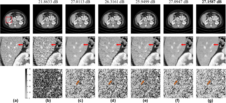
Figure 2: Transverse CT images and corresponding difference images from the Mayo-2016 dataset: (a) NDCT; (b) LDCT; (c) RED-CNN [1]; (d) EDCNN [12]; (e) DU-GAN [9]; (f) ESAU-Net (ours); and (g) ASCON (ours). The display window is [-160, 240] HU.

Qualitative evaluations. Fig. 2 presents qualitative results of three representative methods and our ESAU-Net with MAC-Net on Mayo-2016. Although ASCON and RED-CNN produce visually similar results in low-contrast areas after denoising. However, RED-CNN results in blurred edges between different tissues, such as the liver and blood vessels, while ASCON smoothed the noise and maintained the sharp edges. They are marked by arrows in the regions-of-interest images. We further visualize the corresponding difference images between NDCT and the generated images by our method as well as other methods as shown in the third row of Fig. 2. Note that our ASCON removes more noise components than other methods; refer to Fig. S4 for extra qualitative results on Mayo-2020.

Visualization of inherent semantics. To demonstrate that our MAC-Net can exploit inherent anatomical semantics of CT images during denoising, we select the features before the last layer in ASCON without MAC-Net and ASCON from Mayo-2016. Then we cluster these two feature maps respectively using a K-means algorithm and visualize them in the original dimension, and finally visualize the clustering representations using t-SNE, as shown in Fig. 3. Note that ASCON produces a result similar to organ semantic segmentation after clustering and the intra-class distribution is more compact, as well as the inter-class separation is more obvious. To the best of our knowledge, this is the first time that anatomical semantic information has been demonstrated in a CT denoising task, providing interpretability to the field of medical image reconstruction.

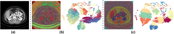
Figure 3: Visualization of inherent semantics; (a) NDCT; (b) clustering and t-SNE results of ASCON w/o MAC-Net; and (c) clustering and t-SNE results of ASCON.

Table 2: Ablation results of Mayo-2020 on the different types of loss functions.

Loss	PSNR$\uparrow$	RMSE$\downarrow$	SSIM$\uparrow$
$\mathcal{L}_{\mathrm{MSE}}$	48.34$\pm$2.22	0.40$\pm$0.11	99.27$\pm$0.18
$\mathcal{L}_{\mathrm{MSE}}+\mathcal{L}_{\mathrm{Perceptual}}$	47.83$\pm$1.99	0.42$\pm$0.10	99.13$\pm$0.19
$\mathcal{L}_{\mathrm{MSE}}+\mathcal{L}_{\mathrm{SSIM}}$	48.31$\pm$1.87	0.40$\pm$0.12	99.30$\pm$0.18
$\mathcal{L}_{\mathrm{MSE}}+\mathcal{L}_{\mathrm{SSIM}}+\mathcal{L}_{\mathrm{global}}$	48.58$\pm$2.12	0.39$\pm$0.10	99.31$\pm$0.17
$\mathcal{L}_{\mathrm{MSE}}+\mathcal{L}_{\mathrm{SSIM}}+\mathcal{L}_{\mathrm{local}}$	48.48$\pm$2.37	0.38$\pm$0.11	99.31$\pm$0.18
$\mathcal{L}_{\mathrm{MSE}}+\mathcal{L}_{\mathrm{SSIM}}+$ $\mathcal{L}_{\mathrm{local}}+\mathcal{L}_{\mathrm{global}}$	48.84$\pm$1.68	0.37$\pm$0.11	99.32$\pm$0.18

Ablation studies. We start with a ESAU-Net using MSE loss and gradually insert some loss functions and our MAC-Net. Table 2 presents the results of different loss functions. It shows that both the global non-contrastive module and local contrastive module are helpful in obtaining better metrics due to the capacity of exploiting inherent anatomical information and maintaining anatomical consistency. Then, we add our MAC-Net to two supervised models: RED-CNN [1] and U-Net [22] but it is less effective, which demonstrates the importance of our ESAU-Net that captures both local and global contexts during denoising in Table S1. In addition, we evaluate the effectiveness of the training strategies including alternate learning, neighboring positive matching and hard negative sampling in Table S2.

4 Conclusion

In this paper, we explore the anatomical semantics in LDCT denoising and take advantage of it to improve the denoising performance. To this end, we propose an Anatomy-aware Supervised CONtrastive learning framework (ASCON), consisting of an efficient self-attention-based U-Net (ESAU-Net) and a multi-scale anatomical contrastive network (MAC-Net), which can capture both local and global contexts during denoising and exploit inherent anatomical information. Extensive experimental results on Mayo-2016 and Mayo-2020 datasets demonstrate the superior performance of our method, and the effectiveness of our designs. We also validated that our method introduces interpretability to LDCT denoising.

Supplementary Materials

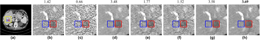
Figure S3: Contrast-to-noise ratio (CNR) of the low-contrast lesion from Mayo-2016 dataset. We select the yellow rectangle of every image to visualize (see in (a)). ROIs of the red rectangle and the blue rectangle are the lesion and the background. (b) NDCT; (c) LDCT; (d) RED-CNN; (e) WGAN-VGG; (f) CNCL; (g) ESAU-Net (ours); and (h) ASCON (ours). Note that our proposed method achieves the best performance of CNR.

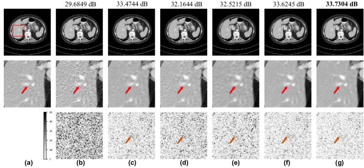
Figure S4: Transverse CT images and corresponding difference images from the Mayo-2020 dataset: (a) NDCT; (b) LDCT; (c) RED-CNN; (d) WGAN-VGG; (e) CNCL; (f) ESAU-Net (ours); and (g) ASCON (ours). Zoomed ROI of the rectangle is shown below the full-size one. The display window is [-160, 240] HU.

Table S1: Ablation results on different supervised models with MAC-Net. Note that the performance of RED-CNN and Unet decreases when adding a MAC-Net. It verifies the importance of our ESAU-Net that captures both local and global contexts during denoising.

		Mayo-2016 Dataset				Mayo-2020 Dataset
Method		PSNR$\uparrow$	RMSE$\downarrow$	SSIM$\uparrow$		PSNR$\uparrow$	RMSE$\downarrow$	SSIM$\uparrow$
RED-CNN		44.23	0.62	97.34		48.05	0.41	99.28
		$\pm$1.26	$\pm$0.09	$\pm$0.86		$\pm$2.14	$\pm$0.11	$\pm$0.18
RED-CNN w/ MAC-Net		43.55	0.67	97.11		47.85	0.42	99.27
		$\pm$1.16	$\pm$0.11	$\pm$0.85		$\pm$2.08	$\pm$0.10	$\pm$0.21
Unet		44.13	0.64	97.38		47.67	0.43	99.19
		$\pm$1.19	$\pm$0.12	$\pm$1.09		$\pm$1.64	$\pm$0.09	$\pm$0.23
Unet w/ MAC-Net		44.04	0.65	97.35		47.66	0.43	99.20
		$\pm$1.15	$\pm$0.11	$\pm$0.98		$\pm$1.82	$\pm$0.10	$\pm$0.21
ESAU-Net		44.38	0.61	97.47		48.31	0.40	99.30
		$\pm$1.26	$\pm$0.09	$\pm$0.87		$\pm$1.87	$\pm$0.12	$\pm$0.18
ASCON (proposed)		44.48	0.60	97.49		48.84	0.37	99.32
		$\pm$1.32	$\pm$0.10	$\pm$0.86		$\pm$1.68	$\pm$0.11	$\pm$0.18

Table S2: Ablation results of Mayo-2020 on the different training strategies in terms of PSNR, RMSE, and SSIM.

Method	PSNR $\uparrow$	RMSE$\downarrow$	SSIM$\uparrow$
w/o alternate training	48.57$\pm$1.82	0.38$\pm$0.10	99.28$\pm$0.19
w/o neighboring positive matching strategy	48.51$\pm$1.61	0.39$\pm$0.10	99.31$\pm$0.17
w/o hard negative sampling	48.41$\pm$1.73	0.40$\pm$0.09	99.29$\pm$0.19
ASCON (proposed)	48.84$\pm$1.68	0.37$\pm$0.11	99.32$\pm$0.18

Algorithm 1 Optimization of alternate learning

1:Input: LDCT $\bm{X}$, NDCT $\bm{Y}$

2:Networks in ASCON: ESAU-Net and MAC-Net

3:Optimizers: Optimizer_E (ESAU-Net) and Optimizer_M (MAC-Net)

4:

5:$\bm{Y}^{\prime}$= ESAU-Net.forward($\bm{X}$)

6:

7:# Optimization of MAC-Net

8:Set_requires_grad (MAC-Net, True)

9:$\operatorname{MAC-Net}$ .forward($\bm{Y}^{\prime}$.detach(), $\bm{Y}$)

10:Optimizer_M.zero_grad()

11:Compute $\mathcal{L}_{\mathrm{contra}}=\mathcal{L}_{\mathrm{local}}+\mathcal{L}_{\mathrm{global}}$

12:$\mathcal{L}_{\mathrm{contra}}$.backward ()

13:Optimizer_M.step ()

14:

15:# Optimization of ESAU-Net

16:Set_requires_grad (MAC-Net, False)

17:Optimizer_E.zero_grad ()

18:Compute $\mathcal{L}=\mathcal{L}_{\mathrm{pixel}}+\mathcal{L}_{\mathrm{contra}}$

19:$\mathcal{L}$.backward ()

20:Optimizer_E.step ()

References

- [1] Chen, H., Zhang, Y., Kalra, M.K., Lin, F., Chen, Y., Liao, P., Zhou, J., Wang, G.: Low-dose CT with a residual encoder-decoder convolutional neural network. IEEE Trans. Med. Imaging 36(12), 2524–2535 (2017)
- [2] Chen, Z., Niu, C., Wang, G., Shan, H.: LIT-Former: Linking in-plane and through-plane transformers for simultaneous CT image denoising and deblurring. arXiv preprint arXiv:2302.10630 (2023)
- [3] Dosovitskiy, A., Beyer, L., Kolesnikov, A., Weissenborn, D., Zhai, X., Unterthiner, T., Dehghani, M., Minderer, M., Heigold, G., Gelly, S., et al.: An image is worth 16x16 words: Transformers for image recognition at scale. arXiv preprint arXiv:2010.11929 (2020)
- [4] Gao, Q., Li, Z., Zhang, J., Zhang, Y., Shan, H.: CoreDiff: Contextual error-modulated generalized diffusion model for low-dose CT denoising and generalization. arXiv preprint arXiv:2304.01814 (2023)
- [5] Gao, Q., Shan, H.: CoCoDiff: a contextual conditional diffusion model for low-dose CT image denoising. In: Developments in X-Ray Tomography XIV. vol. 12242. SPIE (2022)
- [6] Geng, M., Meng, X., Yu, J., Zhu, L., Jin, L., Jiang, Z., Qiu, B., Li, H., Kong, H., Yuan, J., et al.: Content-noise complementary learning for medical image denoising. IEEE Trans. Med. Imaging 41(2), 407–419 (2021)
- [7] Grill, J.B., Strub, F., Altché, F., Tallec, C., Richemond, P., Buchatskaya, E., Doersch, C., Avila Pires, B., Guo, Z., Gheshlaghi Azar, M., et al.: Bootstrap your own latent-a new approach to self-supervised learning. Proc. Adv. Neural Inf. Process. Syst. 33, 21271–21284 (2020)
- [8] He, K., Fan, H., Wu, Y., Xie, S., Girshick, R.: Momentum contrast for unsupervised visual representation learning. In: Proc. IEEE Conf. Comput. Vis. Pattern Recognit. pp. 9729–9738 (2020)
- [9] Huang, Z., Zhang, J., Zhang, Y., Shan, H.: DU-GAN: Generative adversarial networks with dual-domain U-Net-based discriminators for low-dose CT denoising. IEEE Trans. Instrum. Meas. 71, 1–12 (2021)
- [10] Isola, P., Zhu, J.Y., Zhou, T., Efros, A.A.: Image-to-image translation with conditional adversarial networks. In: Proc. IEEE Conf. Comput. Vis. Pattern Recognit. pp. 1125–1134 (2017)
- [11] Johnson, J., Alahi, A., Fei-Fei, L.: Perceptual losses for real-time style transfer and super-resolution. In: Proc. European Conf. Comput. Vis. pp. 694–711. Springer (2016)
- [12] Liang, T., Jin, Y., Li, Y., Wang, T.: EDCNN: Edge enhancement-based densely connected network with compound loss for low-dose CT denoising. In: 2020 15th IEEE Int. Conf. Signal Process. vol. 1, pp. 193–198. IEEE (2020)
- [13] Loshchilov, I., Hutter, F.: SGDR: Stochastic gradient descent with warm restarts. arXiv preprint arXiv:1608.03983 (2016)
- [14] Loshchilov, I., Hutter, F.: Decoupled weight decay regularization. arXiv preprint arXiv:1711.05101 (2017)
- [15] McCollough, C.H., Bartley, A.C., Carter, R.E., Chen, B., Drees, T.A., Edwards, P., Holmes III, D.R., Huang, A.E., Khan, F., Leng, S., et al.: Low-dose CT for the detection and classification of metastatic liver lesions: results of the 2016 low dose CT grand challenge. Med. Phys. 44(10), e339–e352 (2017)
- [16] Moen, T.R., Chen, B., Holmes III, D.R., Duan, X., Yu, Z., Yu, L., Leng, S., Fletcher, J.G., McCollough, C.H.: Low-dose CT image and projection dataset. Med. Phys. 48(2), 902–911 (2021)
- [17] Mussmann, B.R., Mørup, S.D., Skov, P.M., Foley, S., Brenøe, A.S., Eldahl, F., Jørgensen, G.M., Precht, H.: Organ-based tube current modulation in chest CT. a comparison of three vendors. Radiography 27(1), 1–7 (2021)
- [18] Oord, A.v.d., Li, Y., Vinyals, O.: Representation learning with contrastive predictive coding. arXiv preprint arXiv:1807.03748 (2018)
- [19] Park, T., Efros, A.A., Zhang, R., Zhu, J.Y.: Contrastive learning for unpaired image-to-image translation. In: Proc. European Conf. Comput. Vis., Glasgow, UK, August 23–28, 2020, Proceedings, Part IX 16. pp. 319–345. Springer (2020)
- [20] Petit, O., Thome, N., Rambour, C., Themyr, L., Collins, T., Soler, L.: U-net transformer: Self and cross attention for medical image segmentation. In: Mach.Learn. Med. Imag. pp. 267–276. Springer (2021)
- [21] Robinson, J., Chuang, C.Y., Sra, S., Jegelka, S.: Contrastive learning with hard negative samples. arXiv preprint arXiv:2010.04592 (2020)
- [22] Ronneberger, O., Fischer, P., Brox, T.: U-net: Convolutional networks for biomedical image segmentation. In: Med. Image Comput. Comput. Assist. Interv. pp. 234–241. Springer (2015)
- [23] Shan, H., Padole, A., Homayounieh, F., Kruger, U., Khera, R.D., Nitiwarangkul, C., Kalra, M.K., Wang, G.: Competitive performance of a modularized deep neural network compared to commercial algorithms for low-dose CT image reconstruction. Nat. Mach. Intell. 1(6), 269–276 (2019)
- [24] Shan, H., Zhang, Y., Yang, Q., Kruger, U., Kalra, M.K., Sun, L., Cong, W., Wang, G.: 3-D convolutional encoder-decoder network for low-dose CT via transfer learning from a 2-D trained network. IEEE Trans. Med. Imaging 37(6), 1522–1534 (2018)
- [25] Yan, K., Cai, J., Jin, D., Miao, S., Guo, D., Harrison, A.P., Tang, Y., Xiao, J., Lu, J., Lu, L.: SAM: Self-supervised learning of pixel-wise anatomical embeddings in radiological images. IEEE Trans. Med. Imaging 41(10), 2658–2669 (2022)
- [26] Yang, Q., Yan, P., Zhang, Y., Yu, H., Shi, Y., Mou, X., Kalra, M.K., Zhang, Y., Sun, L., Wang, G.: Low-dose CT image denoising using a generative adversarial network with Wasserstein distance and perceptual loss. IEEE Trans. Med. Imaging 37(6), 1348–1357 (2018)
- [27] Yun, S., Lee, H., Kim, J., Shin, J.: Patch-level representation learning for self-supervised vision transformers. In: Proceedings of the IEEE/CVF Conference on Computer Vision and Pattern Recognition. pp. 8354–8363 (2022)
- [28] Zamir, S.W., Arora, A., Khan, S., Hayat, M., Khan, F.S., Yang, M.H.: Restormer: Efficient transformer for high-resolution image restoration. In: Proc. European Conf. Comput. Vis. pp. 5728–5739 (2022)