A Multi-Server Retrial Queueing Inventory System With Asynchronous Multiple Vacations

Abstract

This article deals with asynchronous server vacation and customer retrial facility in a multi-server queueing-inventory system. The Poisson process governs the arrival of a customer. The system is comprised of $c$ identical servers, a finite-size waiting area, and a storage area containing $S$ items. The service time is distributed exponentially. If each server finds that there are an insufficient number of customers and items in the system after the busy period, they start a vacation. Once the server’s vacation is over and it recognizes there is no chance of getting busy, it goes into an idle state if the number of customers or items is not sufficient, otherwise, it will take another vacation. Furthermore, each server’s vacation period occurs independently of the other servers. The system accepts a $(s,Q)$ control policy for inventory replenishment. For the steady-state analysis, the Marcel F Neuts and B Madhu Rao matrix geometric approximation approach is used owing to the structure of an infinitesimal generator matrix. The necessary stability condition and $\mathbb{R}$ matrix are to be computed and presented. After calculating the sufficient system performance measures, an expected total cost of the system is to be constructed and numerically incorporated with the parameters. Additionally, numerical analyses will be conducted to examine the waiting time of customers in the queue and in orbit, as well as the expected rate of customer loss.

Keywords:

Asynchronous multiple vacations, Multi-server, Classical retrial facility, $(s,Q)$ ordering policy

Mathematics Subject classification: 60K25

1 Introduction

Queueing inventory models are more realistic and have more space for study compared to real-world waiting-line systems and servers that are allowed to take vacations. Giving a server time off usually keeps it operating efficiently and increases its lifespan. The continuous operation of a server in the system may cause physical or emotional stress. As a result, the vacation gives the human server a chance to unwind and recharge. Psychiatrists have also claimed that allowing employees to take breaks during their working hours can reduce their stress levels and enhance their productivity.

As per the survey by the Society for Human Resource Management, 67% of businesses provided a bank of paid time off in 2022. The same survey found that 99% of companies offered paid vacations, while only 20% provided paid sick days and paid mental health days, and just 6% offered unlimited paid time off. In 2019, the World at Work Association conducted a poll of employers as part of a study on employee benefits, including the types of paid time off provided. On average, employers offered 17 days of paid time off for workers with less than a year of service, 18 days for those with between one and two years of service, and so on.

As evidenced by the real-world component, research into the queueing-inventory model’s exploration of the vacation process is a necessary area of study. Despite the fact that there are numerous research concepts in the queueing-inventory system regarding the vacation process, the vacation process in multi-server service facilities has not yet been thoroughly researched. This study will thus persuade a multi-server queueing-inventory system’s vacation procedure.

1.1 Motivation

This mathematical model is motivated by a recent visit to a mobile phone store. It works with multiple salespeople to sell mobile phones to arriving customers. During peak hours, the customer arrival rate is higher than during non-peak hours. In such an instant, all sales executives will be busy handling the arriving customers. Due to the long service process, the sales executives feel tired and need some relaxation. Customers are allowed to take a rest period for an exponential amount of time if their arrival rate decreases. After coming back from vacation, they start their work with enthusiasm. The author used this circumstance as inspiration to develop a mathematical model for the stochastic queueing-inventory system.

1.2 Literature Review

The existing literature review of the queueing inventory system(QIS) shows us that, in earlier days, researchers believed that customers received the service immediately after they arrived at the system. Yet, with real-life phenomena, this is not always the case. For instance, when a customer visits a bike showroom, a salesperson usually spends some time explaining the features and benefits of the product. To model such service processes accurately in a stochastic queuing-inventory system (QIS), the concept of positive service time was introduced. This concept was initially proposed by Melikov [1], Sigman and Simchi-Levi [2]. Berman et al. [3] developed a deterministic service time model for a dynamic problem. Several studies have further discussed the concept of positive service time in QIS, including [4, 5, 6, 7].

A customer who attempts to reach customer care but disconnects due to a busy line and then periodically tries again until successfully connected to a server is known as a retrial customer. When the waiting room reaches its maximum capacity, no additional customers will be admitted. They can leave the system for a short period of time to take a break or perform other tasks before rejoining the line. This retry notion is crucial to the study of queueing inventory theory. The retrial concept in inventory systems was first explored by Artaljeo et al. [8]. Paul Manuel et al. [9] investigated a perishable inventory system with a retrial and negative demand. Typically, the retry of a particular client is independent of the other consumers in its orbit. Nevertheless, the rate of retrial consumers is directly proportional to orbit level; this inventory system is known as the "classical retrial inventory system(CRIS)". Ushakumari [10] developed an analytical strategy for CRIS. Nithya et. al. [11] analyzed the two commodities in the single-server QIS with a classical retrial facility.

In the queueing-inventory model, a server is able to take a vacation if it cannot offer the subsequent service. Once the server’s busy phase ends, the server in the system rests for an arbitrary period of time. Practically, allowing the server to take a rest helps it recover its energy and keep offering its services without getting tired. Observing the QIS, the possibility of a server completing his busy period is as follows: 1) When no inventory is available 2) The system does not have any customers. The QIS includes details on the rules for returning from vacations. While completing vacation, the server checks the queue and inventory level. After the vacation is over, the server checks the number of people in line and the number of items in stock. If there are signs that the load is getting heavier, the server will quickly start serving customers again. Otherwise, they may take additional vacations, referred to as multiple vacations. In addition, numerous scholars in the field of QIS have examined other types of vacation, such as delayed vacation, working vacation, differentiated vacation, etc.

Daniel and Ramanarayanan [12] introduced the concept of vacation within a QIS. They used the phrase "rest period" to refer to a server’s vacation time. In [13], it was allowed for the server to take a break once the inventory count reached zero, and it was assumed that the duration of the break followed a general distribution. Any customers who arrive during the server’s break are regarded as lost. In a marketing department, each sales executive is given a monthly target. Once one completes his target, he is allowed to take a vacation. Here, each server can complete its target individually without depending on others. Recently, Yuying Zhang [14] contemplated multiple vacations for a QIS server. The replenishment process was implemented under a random order size policy and the lost sales during the server’s absence were also observed. Dequan Yue and Yaling Qin [15] studied production QIS, assuming that the manufacturing facility would take a vacation when the current inventory level reached $S$ items and would end the vacation as soon as the quantity of inventory items fell below $s$. Similarly, it terminates the vacation whenever the quantity of inventory items falls below $s$. Koroliuk et. al. [16] investigated the QIS server’s vacation assignment. It can be noted that the server is allowed to take a break if there are no customers waiting in the queue, and they also permit the server to terminate their vacation when the queue size reaches a predetermined threshold. Otherwise, his vacation time will be extended. For more details about the QIS with vacation facility, readers can refer to the following papers [17, 18, 19].

Yadavalli and Jeganathan  [20] examined a perishable QIS having dual heterogeneous servers. One of the servers is capable of taking multiple breaks while the other is working. In their research on finite retrial queueing systems with server vacations, Jeganathan et.al [21]) found that utilizing heterogeneous servers was the most effective strategy when compared to using homogeneous servers. Sugapriya et al. [22] analyzed an inventory system where the arrival of customers depends on the number of items in stock and the server takes a vacation when the stock level is empty. Sivakumar [23] studied a retrial inventory system with multiple server vacations, where the server extends the vacation if no items are available in the inventory.

Numerous businesses in the inventory industry concentrate on enhancing their service facilities to meet the demands of their customers. This applies to a variety of establishments, such as car dealerships, clothing stores, jewellery shops, and others that use multi-server service facilities. These real-life scenarios inspired many authors to specialize in stochastic modeling, leading to an interest in increasing the number of servers in the QIS among numerous authors. Krishnamoorthy et al. [24] utilized a multi-server retrial queue in  QIS, and proposed an algorithmic approach for it. Yadavalli et al. discussed a multi-server service facility in their finite population QIS, where a customer enters orbit if all servers are occupied. They applied the Laplace-Stieltjes transform to determine the customer’s unconditional waiting time [25]. Fong-Fan Wang et al. [26] analyzed a priority multi-server service with level-dependent retrial QIS and used a generalized stochastic Petri net to study parameter changes and service rate heterogeneity. Further information on multi-server QIS can be found in the cited papers [27, 28, 29, 30, 31, 32, 33, 34].

Jeganathan et. al. [35] proposed two types of multi-server service facilities to enhance the multi-server QIS by selling and serving items separately. The number of users in the system varies unpredictably and fluctuates between peak and normal hours. For instance, during festivals, more customers visit textile shops than on regular days, while the number of customers is lower on regular days. Meanwhile, Harikrishnan et al. [36] investigated the server activation policy within a queuing-inventory system that features homogeneous servers and multiple threshold stages.

Bright and Taylor [37] analysed the calculation of equilibrium distributions in level-dependent QBD processes and presented algorithms for computing the equilibrium distributions. Zaiming Liu et.al [38] present a detailed analysis of an inventory system in a retrial queue with a level-dependent retrial rate, denoted as $M/PH/1$. They derive several significant findings from their analysis, such as the steady-state probability distribution of inventory levels, the steady-state probability distribution of customers in the system, and the average waiting time of customers in the system. Furthermore, the authors examine the impact of several system parameters, including the arrival rate, service rate, and retrial rate, on system performance. Reshmi and Jose [39] perform a mathematical analysis of a perishable inventory system with dependent retrial loss. According to the authors, the system consists of a single server, an exponential service time, retrials with dependent retrial loss, and a Markovian arrival process (MAP). A $(s,S)$ inventory policy controls the level of inventory, and the demand rate is time-dependent. The study ends with a numerical example that highlights the analytical findings and shows how the dependent retry loss affects the system’s performance. Rejitha and Jose [40] propose a mathematical analysis of a stochastic inventory system with two service modes and customer retrials. The authors characterise the system as a single server with two service modes, fast and slow, with exponentially increasing retrial times. The level of inventory is governed by a $(s,S)$ inventory policy, and the demand rate varies with time. The study concludes with a numerical example that exhibits the influence of the two modalities of service on system performance and displays the analytical results. Narayanan et.al [41] demonstrate that the system has a single server with exponential service time, a vacation period, and a stochastic lead time with correlation. In this paper, the authors analysed the level-dependent quasi-birth-death process and examine the effects of service time, server vacation, and correlated lead time.

1.3 Research Gap

The stochastic queueing-inventory literature has not yet discussed the asynchronous vacation in the multi-server system. To the best of our knowledge, the idea of offering an asynchronous vacation to the servers in the stochastic inventory system is to be considered a research gap in this domain.

1.4 Novelty of the Model

This paper introduces the asynchronous multiple vacation offer to the servers in a multi-server queueing-inventory system (MSQIS). In addition, the servers can do three different jobs: 1. busy; 2. idle; and 3. vacation, according to the situation that occurs in MSQIS. Further, the combination of asynchronous vacation and $(s,Q)$ ordering principle in the MSQIS is also a new attempt.

1.5 Contribution of the Model

The contribution of the paper is described as follows:

1. The considered queueing-inventory system admits asynchronous multiple vacations to its servers when the respective situation occurs.

2. The asynchronous multiple vacation policy is to be applied in the retrial queueing-inventory system.

3. The multi-server vacation queueing-inventory system performs well with the $(s,Q)$ continuous review and reorder setup.

4. This paper finds the stability condition and stationary probability vector using the Neuts and Rao matrix geometric approximation method.

5. This paper explains how to calculate the expected total cost and fraction time of a successful retrial rate for Orbit customers.

6. Further, it investigates the proposed model with some numerical elucidations.

This paper is put together in the following order: notations and model formulation, model analysis and solutions, system performance measures, cost analysis, numerical investigations, and conclusions.

2 Notations and Model Formulation

2.1 Notations

$\begin{array}[]{lcl}{0^{*},Q^{*}}&:&\text{All servers are in vacation mode when the items are $0$ and $Q$ respectively }\\ {\bf 0}&:&\text{A matrix containing all entries are zero}\\ {\bf e}&:&\text{A column vector of appropriate dimensions}\\ &&\text{with each coordinate containing a value of one}\\ I&:&\text{An identity matrix}\\ \delta_{ij}&:&\left\{\begin{array}[]{ll}1,&\mbox{if}\ j=i,\\ 0,&\mbox{otherwise}\end{array}\right.\\ H(x)&:&\left\{\begin{array}[]{ll}1,&\mbox{if}\ x\geq 0,\\ 0,&\mbox{otherwise}\end{array}\right.\\ \lambda&:&\text{Arrival rate of new customer}\\ \theta&:&\text{The rate at which a customer in orbit attempts to retry}\\ \mu&:&\text{The rate at which a customer receives service}\\ \eta&:&\text{Vacation completion rate of a server}\\ \bar{\delta}_{ij}&:&1-\delta_{ij}\\ [D_{l}]_{x,y}&:&\left\{\begin{array}[]{ll}p\lambda,&\mbox{if}\ x=y=l,\\ 0,&\mbox{otherwise~{}~{}~{}~{}~{}~{}~{}~{}~{}~{}~{}~{}~{} where}~{}D_{l}~{}\text{is a matrix of order}~{}l\end{array}\right.\\ [E_{l}]_{x,y}&:&\left\{\begin{array}[]{ll}0,&\mbox{if}\ x=y=l,\\ \iota_{1}\theta,&\mbox{otherwise~{}~{}~{}~{}~{}~{}~{}~{}~{}~{}~{}~{}~{} where}~{}E_{l}~{}\text{ is a matrix of order}~{}l\end{array}\right.\\ P_{1}(t)&:&\text{The number of customers in orbit at time t}\\ P_{2}(t)&:&\text{The level of inventory at time t}\\ P_{3}(t)&:&\text{The number of servers on vacation at time t}\\ P_{4}(t)&:&\text{The number of servers busy with customers at time t.}\\ P_{5}(t)&:&\text{The number of idle servers at the time of t}\\ P_{6}(t)&:&\text{The number of customers in the waiting hall at time t}\\ ch&:&\text{Holding cost per unit item}\\ cs&:&\text{Set up cost per order}\\ co&:&\text{Waiting cost for a customer in the orbit per unit time}\\ cw&:&\text{Waiting cost for a customer in the queue per unit time}\\ cl&:&\text{Lost Cost per customer in the queue per unit time}\end{array}$

Definition 1 (Asynchronous Vacation).

In the system, each server can take or terminate vacation individually; this is called asynchronous vacation.

2.2 Model Formulation

The considered queueing-inventory system explores the performance of a multi-server service facility with asynchronous multiple vacations. Initially, the system has a maximum of $S$ units of an item in the inventory storage space, there is a finite waiting hall of size $N$ and a maximum of $c$ identical servers who can provide service to the customer at an instant. Upon the completion of a customer’s service, one item will be deducted from the inventory storage space.

Depending on the circumstances that arise in the system, servers can perform three different tasks. The following is a list of such jobs: 1. being preoccupied with the customer to close a sale; 2. sitting around in the system; and 3. taking a break from the system.

1. Occurrence of Servers Busy Period: The customer in the queue requires that a number of servers begin to attend if there is a sufficient number of items in the storage space equal to the number of customers in the waiting hall, and vice versa.

2. Occurrence of Servers Idle Period:

   • The server goes to an idle state at the end of each service if the number of customers (except servicing customers) in the queue is insufficient for the number of items (except servicing items) in the storage space, and vice versa.

   • The server goes to idle state at end of the each vacation period if either of the customer level or stock level is insufficient.

3. Occurrence of Servers Vacation Period:

   • The server goes into vacation state at the end of each service if both customer and stock levels in the system (except servicing customers and servicing items) are zero.

   • At the end of each vacation, if the server finds that both customer and stock levels in the system (except servicing customers and servicing items) are zero, then he takes one more vacation.

Customers follow a Poisson distribution when arriving at the waiting hall, with the rate of arrival determined by $\lambda$. If the waiting room is at full capacity, a new customer either enters an infinite capacity orbit with probability $p$, or leaves the system permanently with probability $1-p$. This orbit is a virtual waiting area designed to minimize customer loss in the system. Under the classical retrial policy, any customer from the orbit can enter the waiting hall if the number of customers in the waiting hall is less than $N$. The retrial rate of a customer from the orbit is denoted as $\theta$, and the inter-arrival time between two successful retrial arrivals from the orbit is assumed to be exponentially distributed.

The service time is distributed exponentially and the service rate is defined by the parameter $\mu$. When the system’s current stock level falls to a reorder level of $s$, a reorder of $Q=(S-s)$ items is triggered at that epoch. This kind of reorder process is said to be an $(s,Q)$ replenishment principle. Lead time follows an exponential distribution with the rate $\beta$. The graphical representation is illustrated in Figure (1).

Figure 1: Graphical depiction of the model.

3 Analysis and Solutions of the Model

Consider a six-dimensional Markov process

$$\{P(t)=(P_{1}(t),P_{2}(t),P_{3}(t),P_{4}(t),P_{5}(t),P_{6}(t)),~{}t\geq 0\}$$

with state space $\Omega=\bigcup\limits_{i=1}^{8}E_{i}$ $E_{1}=\left\{(0\leq\iota_{1}<\infty,~{}0,~{}c-x_{1},~{}0,~{}x_{1},~{}x_{1}\leq\iota_{6}\leq N)~{}|~{}0\leq x_{1}\leq c\right\}\\ E_{2}=\left\{(0\leq\iota_{1}<\infty,~{}x_{2}+1,~{}c-(j+1),~{}0\leq\iota_{4}\leq j,~{}j+1-\iota_{4},~{}\iota_{4})~{}|~{}1\leq x_{2}\leq c-2;0\leq j\leq x_{2}-1\right\}\\ E_{3}=\left\{(0\leq\iota_{1}<\infty,~{}x_{2}+1,~{}c-(j+1),~{}j+1,~{}0,~{}j+1\leq\iota_{6}\leq N)~{}|~{}1\leq x_{2}\leq c-2;0\leq j\leq x_{2}-1\right\}\\ E_{4}=\left\{(0\leq\iota_{1}<\infty,~{}j,~{}c-x_{3},~{}0\leq\iota_{4}\leq x_{3}-1,~{}x_{3}-\iota_{4},~{}\iota_{4})~{}|~{}1\leq x_{3}\leq c-1;c\leq j\leq S\right\}\\ E_{5}=\left\{(0\leq\iota_{1}<\infty,~{}j,~{}c-x_{3},~{}x_{3},~{}0,~{}x_{3}\leq\iota_{6}\leq N)~{}|~{}1\leq x_{3}\leq c-1;c\leq j\leq S\right\}\\ E_{6}=\left\{(0\leq\iota_{1}<\infty,~{}Q,~{}c,~{}0,~{}0,~{}0\leq\iota_{6}\leq N)\right\}\\ E_{7}=\left\{(0\leq\iota_{1}<\infty,~{}x_{4}+1,~{}c-(x_{4}+1),~{}0\leq\iota_{4}\leq x_{4},~{}x_{4}+1-\iota_{4},~{}\iota_{4})~{}|~{}0\leq x_{4}\leq c-1\right\}\\ E_{8}=\left\{(0\leq\iota_{1}<\infty,~{}x_{5},~{}c-x_{5},~{}x_{5},~{}0,~{}x_{5}\leq\iota_{6}\leq N)~{}|~{}1\leq x_{5}\leq c\right\}\\ E_{9}=\left\{(0\leq\iota_{1}<\infty,~{}x_{6},~{}c-(x_{6}+j),~{}x_{6},~{}j,~{}(x_{6}+j)\leq\iota_{6}\leq N)~{}|~{}1\leq x_{6}\leq c-1;1\leq j\leq c-x_{6}\right\}\\ E_{10}=\left\{(0\leq\iota_{1}<\infty,~{}x_{7},~{}0,~{}0\leq\iota_{4}\leq c-1,~{}c-\iota_{4},~{}\iota_{4})~{}|~{}c+1\leq x_{6}\leq S\right\}\\ E_{11}=\left\{(0\leq\iota_{1}<\infty,~{}x_{7},~{}0,~{}c,~{}0,~{}c\leq\iota_{6}\leq N)~{}|~{}c+1\leq x_{7}\leq S\right\}$

3.1 Construction of Infinitesimal Generator Matrix

The process $\{P(t),t\geq 0\}$ is called a $QBD$ process and its infinitesimal generator matrix is given by

$$H = \left(\begin{array}[]{cccccccccccccccccccccc}{\mathbb{H}_{01}}&\mathbb{H}_{0}&\mathbf{0}&\mathbf{0}&\mathbf{0}&\cdots\\ \mathbb{H}_{10}&\mathbb{H}_{11}&\mathbb{H}_{0}&\mathbf{0}&\mathbf{0}&\cdots\\ \mathbf{0}&\mathbb{H}_{20}&\mathbb{H}_{21}&\mathbb{H}_{0}&\mathbf{0}&\cdots\\ \vdots&\vdots&\vdots&\vdots&\vdots&\ddots\\ \end{array}\right),$$ (3.5)

where all the matrices in the above infinitesimal generator matrix $H$ have dimension

$$Sc(N+1)+(c+2)N-(2c^{3}+3c^{2}-5c-12)(1/6)$$

and all the sub-matrices are defined as follows:

1. The non-zero upper diagonal matrix, $\mathbb{H}_{0}$ describes the transitions of the new arrival to the orbit if the waiting hall is full.

   $$\mathbb{H}_{0} = diag(\Bbbk_{0^{*}},\Bbbk_{Q^{*}},\Bbbk_{0},\Bbbk_{1},\cdots,\Bbbk_{c-1},\Bbbk_{c},\Bbbk_{c},\cdots,\Bbbk_{c})$$ (3.6)

   where

   $$\Bbbk_{j}=diag(D_{N-(c-1)},D_{N-(c-2)},\cdots,D_{N-j},D_{N+1},D_{N+1},\cdots,D_{N+1}),~{}j=0,1,\cdots,c$$ (3.7)

   is a sub-block matrix of order $c$.

2. The non-zero lower diagonal matrix, $\mathbb{H}_{\iota_{1}0}$ denotes the transitions of orbit customers enter the waiting hall.

   $$\text{For}~{}~{}\iota_{1}=1,2,\cdots$$

   $$\mathbb{H}_{\iota_{1}0} = diag(\mathbb{W}_{0^{*}},\mathbb{W}_{Q^{*}},\mathbb{W}_{0},\mathbb{W}_{1},\cdots,\mathbb{W}_{c-1},\mathbb{W}_{c},\mathbb{W}_{c},\cdots,\mathbb{W}_{c})$$ (3.8)

   where

   $$\mathbb{W}_{j}=diag(E_{N-(c-1)},E_{N-(c-2)},\cdots,E_{N-j},E_{N+1},E_{N+1},\cdots,E_{N+1}),~{}j=0,1,\cdots,c$$ (3.9)

   is a sub-block matrix of order $c$.

3. The diagonal matrix, $\mathbb{H}_{\iota_{1}1}$ describes the transitions of primary arrival, service process, reorder process, server taking a vacation and vacation completion process.

   $$\text{For}~{}~{}\iota_{1}=0,1,2,\cdots$$

   $$\left[\mathbb{H}_{\iota_{1}1}\right]_{\iota_{2},\iota_{2}^{{}^{\prime}}} = \left\{\begin{array}[]{llll}\mathbb{J}_{\iota_{2}^{{}^{\prime}}}&\iota_{2}^{{}^{\prime}}=0^{*}&\iota_{2}=1\\ \mathbb{J}_{\iota_{2}^{{}^{\prime}}}&\iota_{2}^{{}^{\prime}}=Q^{*},0&\iota_{2}=0^{*}\\ \mathbb{J}_{\iota_{2}^{{}^{\prime}}}&\iota_{2}^{{}^{\prime}}=Q&\iota_{2}=Q^{*}\\ \mathbb{F}_{\iota_{2}}&\iota_{2}^{{}^{\prime}}=\iota_{2}-1&\iota_{2}\in 1,2,\cdots,c\\ \mathbb{F}_{c+1}&\iota_{2}^{{}^{\prime}}=\iota_{2}-1&\iota_{2}\in c+1,c+2,\cdots,S\\ \mathbb{L}_{\iota_{2}}&\iota_{2}^{{}^{\prime}}=\iota_{2}+Q&\iota_{2}\in 0,1,2,\cdots,c\\ \mathbb{L}_{c}&\iota_{2}^{{}^{\prime}}=\iota_{2}+Q&\iota_{2}\in c+1,c+2,\cdots,s\\ \mathbb{G}_{\iota_{2}^{{}^{\prime}}}&\iota_{2}^{{}^{\prime}}=\iota_{2}&\iota_{2}\in 0^{*},Q^{*},0,1,\cdots,c-1\\ \mathbb{G}_{c}&\iota_{2}^{{}^{\prime}}=\iota_{2}&\iota_{2}\in c,c+1,\cdots,S\\ 0,&\mbox{otherwise}\end{array}\right.$$ (3.20)

   where

   $$\mathbb{J}_{0^{*}} = \left\{\begin{array}[]{llllll}\iota_{4}\mu&\iota_{3}=c-1&\iota_{4}=1&\iota_{5}=0&\iota_{6}=1,2,\cdots,N\\ &\iota_{3}^{{}^{\prime}}=c&\iota_{4}^{{}^{\prime}}=0&\iota_{5}^{{}^{\prime}}=\iota_{5}&\iota_{6}^{{}^{\prime}}=\iota_{6}-1\\ 0,&\mbox{otherwise,}\end{array}\right.$$ (3.24)

   $$\mathbb{J}_{Q^{*}} = \left\{\begin{array}[]{llllll}\beta&\iota_{3}=c&\iota_{4}=0&\iota_{5}=0&\iota_{6}=0,1,2,\cdots,N\\ &\iota_{3}^{{}^{\prime}}=c&\iota_{4}^{{}^{\prime}}=\iota_{4}&\iota_{5}^{{}^{\prime}}=\iota_{5}&\iota_{6}^{{}^{\prime}}=\iota_{6}\\ 0,&\mbox{otherwise,}\end{array}\right.$$ (3.28)

   $$\mathbb{J}_{0} = \left\{\begin{array}[]{llllll}\eta&\iota_{3}=c&\iota_{4}=0&\iota_{5}=0&\iota_{6}=1,2,\cdots,N\\ &\iota_{3}^{{}^{\prime}}=c-1&\iota_{4}^{{}^{\prime}}=\iota_{4}&\iota_{5}^{{}^{\prime}}=1&\iota_{6}^{{}^{\prime}}=\iota_{6}\\ 0,&\mbox{otherwise,}\end{array}\right.$$ (3.32)

   $$\mathbb{J}_{Q} = \left\{\begin{array}[]{llllll}\eta&\iota_{3}=c&\iota_{4}=0&\iota_{5}=0&\iota_{6}=0,1,2,\cdots,N\\ &\iota_{3}^{{}^{\prime}}=c-1&\iota_{4}^{{}^{\prime}}=1-\iota_{5}^{{}^{\prime}}&\iota_{5}^{{}^{\prime}}=\delta_{\iota_{6}^{{}^{\prime}}0}&\iota_{6}^{{}^{\prime}}=\iota_{6}\\ 0,&\mbox{otherwise,}\end{array}\right.$$ (3.36)

   For $\iota_{2}\in 1,2,\cdots,c-1$

   $$\mathbb{F}_{\iota_{2}} = \left\{\begin{array}[]{lllllll}\iota_{4}\mu&\iota_{3}=0,\cdots,c-(\iota_{2}+1)&\iota_{4}=\iota_{2}&\iota_{5}=c-(\iota_{3}+\iota_{4})&\iota_{6}=\iota_{4}+\iota_{5}\\ &\iota_{3}^{{}^{\prime}}=\iota_{3}+1&\iota_{4}^{{}^{\prime}}=\iota_{4}-1&\iota_{5}^{{}^{\prime}}=\iota_{5}&\iota_{6}^{{}^{\prime}}=\iota_{6}-1\\ \iota_{4}\mu&\iota_{3}=0,\cdots,c-(\iota_{2}+1)&\iota_{4}=\iota_{2}&\iota_{5}=c-(\iota_{3}+\iota_{4})&\iota_{6}=\iota_{4}+\iota_{5}+1,\cdots,N\\ &\iota_{3}^{{}^{\prime}}=\iota_{3}&\iota_{4}^{{}^{\prime}}=\iota_{4}-1&\iota_{5}^{{}^{\prime}}=\iota_{5}+1&\iota_{6}^{{}^{\prime}}=\iota_{6}-1\\ \bar{\delta}_{\iota_{2}1}\iota_{4}\mu&\iota_{3}=c-\iota_{2},\cdots,c-2&\iota_{4}=1,\cdots,c-\iota_{3}&\iota_{5}=c-(\iota_{3}+\iota_{4})&\iota_{6}=\iota_{4}\\ &\iota_{3}^{{}^{\prime}}=\iota_{3}+1&\iota_{4}^{{}^{\prime}}=\iota_{4}-1&\iota_{5}^{{}^{\prime}}=\iota_{5}&\iota_{6}^{{}^{\prime}}=\iota_{6}-1\\ \bar{\delta}_{\iota_{2}1}\iota_{4}\mu&\iota_{3}=c-\iota_{2},\cdots,c-2&\iota_{4}=\iota_{2}&\iota_{5}=0&\iota_{6}=c-\iota_{3},\cdots,N\\ &\iota_{3}^{{}^{\prime}}=\iota_{3}&\iota_{4}^{{}^{\prime}}=\iota_{4}-1&\iota_{5}^{{}^{\prime}}=\iota_{5}+1&\iota_{6}^{{}^{\prime}}=\iota_{6}-1\\ \iota_{4}\mu&\iota_{3}=c-1&\iota_{4}=1&\iota_{5}=0&\iota_{6}=1,2,\cdots,N\\ &\iota_{3}^{{}^{\prime}}=\iota_{3}&\iota_{4}^{{}^{\prime}}=\delta_{\iota_{6}^{{}^{\prime}}2}&\iota_{5}^{{}^{\prime}}=\delta_{\iota_{6}^{{}^{\prime}}1}&\iota_{6}^{{}^{\prime}}=\iota_{6}-1\\ 0,&\mbox{otherwise,}\end{array}\right.$$ (3.48)

   $$\mathbb{F}_{c} = \left\{\begin{array}[]{lllllll}\iota_{4}\mu&\iota_{3}=0&\iota_{4}=1,\cdots,c&\iota_{5}=c-\iota_{4}&\iota_{6}=\iota_{4}\\ &\iota_{3}^{{}^{\prime}}=1&\iota_{4}^{{}^{\prime}}=\iota_{4}-1&\iota_{5}^{{}^{\prime}}=\iota_{5}-1&\iota_{6}^{{}^{\prime}}=\iota_{6}-1\\ \iota_{4}\mu&\iota_{3}=0&\iota_{4}=c&\iota_{5}=0&\iota_{6}=c+1,\cdots,N\\ &\iota_{3}^{{}^{\prime}}=\iota_{3}&\iota_{4}^{{}^{\prime}}=\iota_{4}-1&\iota_{5}^{{}^{\prime}}=1&\iota_{6}^{{}^{\prime}}=\iota_{6}-1\\ \iota_{4}\mu&\iota_{3}=1,\cdots,c-1&\iota_{4}=1,\cdots,c-\iota_{3}&\iota_{5}=c-(\iota_{3}+\iota_{4})&\iota_{6}=\iota_{4}\\ &\iota_{3}^{{}^{\prime}}=\iota_{3}&\iota_{4}^{{}^{\prime}}=\iota_{4}-1&\iota_{5}^{{}^{\prime}}=\iota_{5}+1&\iota_{6}^{{}^{\prime}}=\iota_{6}-1\\ \iota_{4}\mu&\iota_{3}=1,\cdots,c-1&\iota_{4}=c-\iota_{3}&\iota_{5}=0&\iota_{6}=\iota_{4}+1,\cdots,N\\ &\iota_{3}^{{}^{\prime}}=\iota_{3}&\iota_{4}^{{}^{\prime}}=\iota_{4}&\iota_{5}^{{}^{\prime}}=\iota_{5}&\iota_{6}^{{}^{\prime}}=\iota_{6}-1\\ 0,&\mbox{otherwise,}\end{array}\right.$$ (3.59)

   For $\iota_{2}\in c+1,c+2,\cdots,S$

   $$\mathbb{F}_{c+1} = \left\{\begin{array}[]{lllllll}\iota_{4}\mu&\iota_{3}=0,1,\cdots,c-1&\iota_{4}=1,\cdots,c-\iota_{3}&\iota_{5}=c-(\iota_{3}+\iota_{4})&\iota_{6}=\iota_{4}\\ &\iota_{3}^{{}^{\prime}}=\iota_{3}&\iota_{4}^{{}^{\prime}}=\iota_{4}-1&\iota_{5}^{{}^{\prime}}=\iota_{5}+1&\iota_{6}^{{}^{\prime}}=\iota_{6}-1\\ \iota_{4}\mu&\iota_{3}=0,1,\cdots,c-1&\iota_{4}=c-\iota_{3}&\iota_{5}=0&\iota_{6}=\iota_{4}+1,\cdots,N\\ &\iota_{3}^{{}^{\prime}}=\iota_{3}&\iota_{4}^{{}^{\prime}}=\iota_{4}&\iota_{5}^{{}^{\prime}}=\iota_{5}&\iota_{6}^{{}^{\prime}}=\iota_{6}-1\\ 0,&\mbox{otherwise,}\end{array}\right.$$ (3.66)

   For $\iota_{2}\in 0,1,\cdots,c-1$

   $$\mathbb{L}_{\iota_{2}} = \left\{\begin{array}[]{lllllll}\beta&\iota_{3}=0,\cdots,c-(\iota_{2}+1)&\iota_{4}=\iota_{2}&\iota_{5}=c-(\iota_{3}+\iota_{4})&\iota_{6}=\iota_{4}+\iota_{5},\cdots,N\\ &\iota_{3}^{{}^{\prime}}=\iota_{3}&\iota_{4}^{{}^{\prime}}=c-\iota_{3}^{{}^{\prime}}&\iota_{5}^{{}^{\prime}}=0&\iota_{6}^{{}^{\prime}}=\iota_{6}\\ \bar{\delta}_{\iota_{2}0}\beta&\iota_{3}=c-\iota_{2},\cdots,c-1&\iota_{4}=0,\cdots,c-\iota_{3}&\iota_{5}=c-(\iota_{3}+\iota_{4})&\iota_{6}=\iota_{4}\\ &\iota_{3}^{{}^{\prime}}=\iota_{3}&\iota_{4}^{{}^{\prime}}=\iota_{4}&\iota_{5}^{{}^{\prime}}=\iota_{5}&\iota_{6}^{{}^{\prime}}=\iota_{6}\\ \bar{\delta}_{\iota_{2}0}\beta&\iota_{3}=c-\iota_{2},\cdots,c-1&\iota_{4}=\iota_{2}&\iota_{5}=0&\iota_{6}=c-\iota_{3}+1,\cdots,N\\ &\iota_{3}^{{}^{\prime}}=\iota_{3}&\iota_{4}^{{}^{\prime}}=\iota_{4}&\iota_{5}^{{}^{\prime}}=\iota_{5}&\iota_{6}^{{}^{\prime}}=\iota_{6}\\ 0,&\mbox{otherwise,}\end{array}\right.$$ (3.75)

   $$\mathbb{L}_{c} = \left\{\begin{array}[]{lllllll}\beta&\iota_{3}=0,\cdots,c-1&\iota_{4}=0,\cdots,c-\iota_{3}&\iota_{5}=c-(\iota_{3}+\iota_{4})&\iota_{6}=\iota_{4}\\ &\iota_{3}^{{}^{\prime}}=\iota_{3}&\iota_{4}^{{}^{\prime}}=\iota_{4}&\iota_{5}^{{}^{\prime}}=\iota_{5}&\iota_{6}^{{}^{\prime}}=\iota_{6}\\ \beta&\iota_{3}=0,\cdots,c-1&\iota_{4}=c-\iota_{3}&\iota_{5}=0&\iota_{6}=\iota_{4}+1,\cdots,N\\ &\iota_{3}^{{}^{\prime}}=\iota_{3}&\iota_{4}^{{}^{\prime}}=\iota_{4}&\iota_{5}^{{}^{\prime}}=\iota_{5}&\iota_{6}^{{}^{\prime}}=\iota_{6}\\ 0,&\mbox{otherwise,}\end{array}\right.$$ (3.82)

   For $\iota_{2}\in 0^{*},Q^{*}$

   $$\mathbb{G}_{\iota_{2}} = \left\{\begin{array}[]{llllll}-(\iota_{1}\theta+\bar{\delta}_{\iota_{6}N}\lambda+\delta_{\iota_{2}0^{*}}~{}\beta+\delta_{\iota_{2}0^{*}}\bar{\delta}_{\iota_{6}N}~{}\eta&&&&\\ +\delta_{\iota_{2}Q^{*}}~{}\eta+\delta_{\iota_{6}N}~{}p\lambda)&\iota_{3}=c&\iota_{4}=0&\iota_{5}=0&\iota_{6}=0,1,\cdots,N\\ &\iota_{3}^{{}^{\prime}}=c&\iota_{4}^{{}^{\prime}}=\iota_{4}&\iota_{5}^{{}^{\prime}}=\iota_{5}&\iota_{6}^{{}^{\prime}}=\iota_{6}\\ \lambda&\iota_{3}=c&\iota_{4}=0&\iota_{5}=0&\iota_{6}=0,1,\cdots,N-1\\ &\iota_{3}^{{}^{\prime}}=c&\iota_{4}^{{}^{\prime}}=\iota_{4}&\iota_{5}^{{}^{\prime}}=\iota_{5}&\iota_{6}^{{}^{\prime}}=\iota_{6}+1\\ 0,&\mbox{otherwise,}\end{array}\right.$$ (3.90)

   For $\iota_{2}\in 0,1,\cdots,c-1$

   $$\mathbb{G}_{\iota_{2}}=\left\{\begin{array}[]{lllllll}\lambda&0\leq\iota_{3}\leq c-(\iota_{2}+1)&\iota_{4}=\iota_{2}&\iota_{5}=c-(\iota_{3}+\iota_{4})&\iota_{4}+\iota_{5}\leq\iota_{6}\leq N-1\\ &\iota_{3}^{{}^{\prime}}=\iota_{3}&\iota_{4}^{{}^{\prime}}=\iota_{4}&\iota_{5}^{{}^{\prime}}=\iota_{5}&\iota_{6}^{{}^{\prime}}=\iota_{6}+1\\ \bar{\delta}_{\iota_{2}0}\lambda&c-\iota_{2}\leq\iota_{3}\leq c-1&0\leq\iota_{4}\leq c-\iota_{3}&\iota_{5}=c-(\iota_{3}+\iota_{4})&\iota_{6}=\iota_{4}\\ &\iota_{3}^{{}^{\prime}}=\iota_{3}&\iota_{4}^{{}^{\prime}}=\iota_{4}&\iota_{5}^{{}^{\prime}}=\iota_{5}&\iota_{6}^{{}^{\prime}}=\iota_{6}+1\\ \bar{\delta}_{\iota_{2}0}\lambda&c-\iota_{2}\leq\iota_{3}\leq c-1&\iota_{4}=\iota_{2}&\iota_{5}=0&c-\iota_{3}+1\leq\iota_{6}\leq N-1\\ &\iota_{3}^{{}^{\prime}}=\iota_{3}&\iota_{4}^{{}^{\prime}}=\iota_{4}&\iota_{5}^{{}^{\prime}}=\iota_{5}&\iota_{6}^{{}^{\prime}}=\iota_{6}+1\\ -(\iota_{4}\mu&&&&\\ +\bar{\delta}_{\iota_{6}N}(\lambda+\iota_{1}\theta)&&&&\\ +\bar{\delta}_{\iota_{3}0}\bar{\delta}_{\iota_{6}\iota_{5}}\eta&&&&\\ +\delta_{\iota_{6}N}~{}p\lambda)&0\leq\iota_{3}\leq c-(\iota_{2}+1)&\iota_{4}=\iota_{2}&\iota_{5}=c-(\iota_{3}+\iota_{4})&\iota_{4}+\iota_{5}\leq\iota_{6}\leq N\\ &\iota_{3}^{{}^{\prime}}=\iota_{3}&\iota_{4}^{{}^{\prime}}=\iota_{4}&\iota_{5}^{{}^{\prime}}=\iota_{5}&\iota_{6}^{{}^{\prime}}=\iota_{6}\\ -\bar{\delta}_{\iota_{2}0}(\iota_{4}\mu+&&&&\\ (\lambda+\iota_{1}\theta)+&&&&\\ \bar{\delta}_{\iota_{2}(c-1)}\bar{\delta}_{\iota_{3}(c-1)}\eta&&&&\\ +\delta_{\iota_{6}N}~{}p\lambda)&c-\iota_{2}\leq\iota_{3}\leq c-1&0\leq\iota_{4}\leq c-\iota_{3}&\iota_{5}=c-(\iota_{3}+\iota_{4})&\iota_{6}=\iota_{4}\\ &\iota_{3}^{{}^{\prime}}=\iota_{3}&\iota_{4}^{{}^{\prime}}=\iota_{4}&\iota_{5}^{{}^{\prime}}=\iota_{5}&\iota_{6}^{{}^{\prime}}=\iota_{6}\\ -\bar{\delta}_{\iota_{2}0}(\iota_{4}\mu+&&&&\\ \bar{\delta}_{\iota_{6}N}(\lambda+\iota_{1}\theta)&&&&\\ +\eta+\delta_{\iota_{6}N}~{}p\lambda)&c-\iota_{2}\leq\iota_{3}\leq c-1&\iota_{4}=\iota_{2}&\iota_{5}=0&\iota_{2}+1\leq\iota_{6}\leq N\\ &\iota_{3}^{{}^{\prime}}=\iota_{3}&\iota_{4}^{{}^{\prime}}=\iota_{4}&\iota_{5}^{{}^{\prime}}=\iota_{5}&\iota_{6}^{{}^{\prime}}=\iota_{6}\\ 0,&\mbox{otherwise.}\end{array}\right.$$ (3.113)

   For $\iota_{2}\in c,c+1,\cdots,S$

   $$\mathbb{G}_{c}=\left\{\begin{array}[]{lllllll}-(\iota_{4}\mu+\delta_{\iota_{3}0}~{}\eta&&&&\\ +\lambda+\iota_{1}\theta)&0\leq\iota_{3}\leq c-1&0\leq\iota_{4}\leq c-\iota_{3}&\iota_{5}=c-(\iota_{3}+\iota_{4})&\iota_{6}=\iota_{4}\\ &\iota_{3}^{{}^{\prime}}=\iota_{3}&\iota_{4}^{{}^{\prime}}=\iota_{4}&\iota_{5}^{{}^{\prime}}=\iota_{5}&\iota_{6}^{{}^{\prime}}=\iota_{6}\\ -(\iota_{4}\mu+\eta&&&&\\ +\bar{\delta}_{\iota_{6}N}(\lambda+\iota_{1}\theta)&&&&\\ +\delta_{\iota_{6}N}~{}p\lambda)&0\leq\iota_{3}\leq c-1&\iota_{4}=c-\iota_{3}&\iota_{5}=0&c-\iota_{3}+1\leq\iota_{6}\leq N\\ &\iota_{3}^{{}^{\prime}}=\iota_{3}&\iota_{4}^{{}^{\prime}}=\iota_{4}&\iota_{5}^{{}^{\prime}}=\iota_{5}&\iota_{6}^{{}^{\prime}}=\iota_{6}\\ \lambda&0\leq\iota_{3}\leq c-1&0\leq\iota_{4}\leq c-\iota_{3}&\iota_{5}=c-(\iota_{3}+\iota_{4})&\iota_{6}=\iota_{4}\\ &\iota_{3}^{{}^{\prime}}=\iota_{3}&\iota_{4}^{{}^{\prime}}=\iota_{4}&\iota_{5}^{{}^{\prime}}=\iota_{5}&\iota_{6}^{{}^{\prime}}=\iota_{6}+1\\ \lambda&0\leq\iota_{3}\leq c-1&\iota_{4}=c-\iota_{3}&\iota_{5}=0&c-\iota_{3}+1\leq\iota_{6}\leq N-1\\ &\iota_{3}^{{}^{\prime}}=\iota_{3}&\iota_{4}^{{}^{\prime}}=\iota_{4}&\iota_{5}^{{}^{\prime}}=\iota_{5}&\iota_{6}^{{}^{\prime}}=\iota_{6}+1\\ 0,&\mbox{otherwise,}\end{array}\right.$$ (3.127)

The ergodicity of the Markov chain $P(t)$ is assumed to $\rho=\dfrac{\lambda}{c\mu}<1\text{(See ~{}\cite[cite]{[\@@bibref{}{arpo}{}{}]})}$.

3.2 Neuts and Rao Matrix Geometric Approximation

As the assumed Markov chain $\{P(t),t\geq 0\}$ has the structure of a level-dependent QBD process, it is hard to find the steady-state probability vector analytically. So we truncate the orbit level at the point $M$. The truncation point is defined as the point $M$, where $M\geq 1$ in which the system changes itself from level-dependent QBD to level-independent QBD when $\iota_{1}<M$ and $\iota_{1}\geq M$, respectively. More explicitly, by setting $\mathbb{H}_{\iota_{1}0}=\mathbb{H}_{M0}$ and $\mathbb{H}_{\iota_{1}1}=\mathbb{H}_{M1}$ for all $\iota_{1}\geq M$, we determine the equilibrium for the considered system. The choice of the truncated value $M$ is determined according to Marcel F Neuts and B M Rao [43] and Srinivas R Chakravarthy et.al [44].

The determination of the modified infinitesimal generator structure of $H$ is based on the Neuts and Rao matrix geometric approximation method [43] and it is determined as follows:

$$\hat{H} = \left(\begin{array}[]{cccccccccccccccccccccc}{\mathbb{H}_{01}}&\mathbb{H}_{0}&\mathbf{0}&\mathbf{0}&\mathbf{0}&\cdots&\mathbf{0}&\mathbf{0}&\mathbf{0}&\mathbf{0}&\mathbf{0}&\cdots\\ \mathbb{H}_{10}&\mathbb{H}_{11}&\mathbb{H}_{0}&\mathbf{0}&\mathbf{0}&\cdots&\mathbf{0}&\mathbf{0}&\mathbf{0}&\mathbf{0}&\mathbf{0}&\cdots\\ \mathbf{0}&\mathbb{H}_{20}&\mathbb{H}_{21}&\mathbb{H}_{0}&\mathbf{0}&\cdots&\mathbf{0}&\mathbf{0}&\mathbf{0}&\mathbf{0}&\mathbf{0}&\cdots\\ \vdots&\vdots&\vdots&\vdots&\vdots&\ddots&\vdots&\vdots&\vdots&\vdots&\vdots&\ddots\\ \mathbf{0}&\mathbf{0}&\mathbf{0}&\mathbf{0}&\mathbf{0}&\cdots&\mathbb{H}_{M0}&\mathbb{H}_{M1}&\mathbb{H}_{0}&\mathbf{0}&\mathbf{0}&\cdots\\ \mathbf{0}&\mathbf{0}&\mathbf{0}&\mathbf{0}&\mathbf{0}&\cdots&\mathbf{0}&\mathbb{H}_{M0}&\mathbb{H}_{M1}&\mathbb{H}_{0}&\mathbf{0}&\cdots\\ \vdots&\vdots&\vdots&\vdots&\vdots&\ddots&\vdots&\vdots&\vdots&\vdots&\vdots&\ddots\\ \end{array}\right),$$

Theorem 2.

The probability vector $\phi$ in steady-state, which is related to the finite generator matrix $\mathbb{H}_{M}$ at truncation point $M$, can be obtained from the following equation: $\mathbb{H}_{M}\phi=0$, where $\mathbb{H}_{M}=\mathbb{H}_{M0}+\mathbb{H}_{M1}+\mathbb{H}_{0}$ and the vector $\phi$ as converted as follows:

$${\phi^{(\iota_{2})}} = {\phi^{(Q)}}{\nabla_{\iota_{2}}},\quad\iota_{2}=0^{*},Q^{*},0,1,\ldots,S.$$ (3.130)

where

$$\nabla_{\iota_{2}}=\left\{\begin{array}[]{lll}(-1)^{Q}(\mathbb{F}_{c+1}\mathbb{\hat{G}}_{c}^{-1})^{Q-c}\left(\prod\limits_{i=1}^{c-1}\mathbb{F}_{i+1}\mathbb{\hat{G}}_{i}^{-1}\right)\mathbb{J}_{\iota_{2}}\mathbb{\hat{G}}_{\iota_{2}}^{-1}&\iota_{2}=0^{*}\\ (-1)^{Q+1}(\mathbb{F}_{c+1}\mathbb{\hat{G}}_{c}^{-1})^{Q-c}\left(\prod\limits_{i=1}^{c-1}\mathbb{F}_{i+1}\mathbb{\hat{G}}_{i}^{-1}\right)\mathbb{J}_{0^{*}}\mathbb{\hat{G}}_{0^{*}}^{-1}\mathbb{J}_{\iota_{2}}\mathbb{\hat{G}}_{\iota_{2}}^{-1}&\iota_{2}=Q^{*}\\ (-1)^{Q}(\mathbb{F}_{c+1}\mathbb{\hat{G}}_{c}^{-1})^{Q-c}\left(\prod\limits_{i=1}^{c-1}\mathbb{F}_{i+1}\mathbb{\hat{G}}_{i}^{-1}\right)\left(\mathbb{F}_{1}G_{0}^{-1}-\mathbb{J}_{0^{*}}\mathbb{\hat{G}}_{0^{*}}^{-1}\mathbb{J}_{0}\mathbb{\hat{G}}_{0}^{-1}\right)&\iota_{2}=0\\ (-1)^{Q-\iota_{2}}(\mathbb{F}_{c+1}\mathbb{\hat{G}}_{c}^{-1})^{Q-c}\left(\prod\limits_{i=\iota_{2}}^{c-1}\mathbb{F}_{i+1}\mathbb{\hat{G}}_{i}^{-1}\right)&\iota_{2}\in 1,2,\cdots,c-1\\ (-1)^{Q-\iota_{2}}(\mathbb{F}_{c+1}\mathbb{\hat{G}}_{c}^{-1})^{Q-\iota_{2}}&\iota_{2}\in c,c+1,\cdots,S\\ I&\iota_{2}=Q\\ (-1)^{Q-(j-1)}(\mathbb{F}_{c+1}\mathbb{\hat{G}}_{c}^{-1})^{Q-s}&\\ \Biggl{[}\sum\limits_{x=j+1}^{c}\left((\mathbb{F}_{c+1}\mathbb{\hat{G}}_{c}^{-1})^{s-c}\left(\prod\limits_{i=c}^{k}\mathbb{F}_{i}\mathbb{\hat{G}}_{i-1}^{-1}\right)\mathbb{L}_{k}\mathbb{\hat{G}}_{c}^{-1}(\mathbb{F}_{c+1}\mathbb{\hat{G}}_{c}^{-1})^{x-(j+1)}\right)+&\\ \left(\sum\limits_{x=0}^{s-c}(\mathbb{F}_{c+1}\mathbb{\hat{G}}_{c}^{-1})^{s-c-x}\mathbb{L}_{c}\mathbb{\hat{G}}_{c}^{-1}(\mathbb{F}_{c+1}\mathbb{\hat{G}}_{c}^{-1})^{x}\right)(\mathbb{F}_{c+1}\mathbb{\hat{G}}_{c}^{-1})^{c-j}\Biggr{]}&\iota_{2}\in Q+j,\\ &j\in 1,2,\cdots,c-1\\ (-1)^{Q-(j-1)}(\mathbb{F}_{c+1}\mathbb{\hat{G}}_{c}^{-1})^{Q-s}\left\{\sum\limits_{x=0}^{s-j}(\mathbb{F}_{c+1}\mathbb{\hat{G}}_{c}^{-1})^{s-j-x}\mathbb{L}_{c}\mathbb{\hat{G}}_{c}^{-1}(\mathbb{F}_{c+1}\mathbb{\hat{G}}_{c}^{-1})^{x}\right\}&\iota_{2}\in Q+j,\\ &j\in c,c+1,\cdots,S\\ 0,&\mbox{otherwise}\end{array}\right.$$

and ${\phi^{(Q)}}$ is obtained by solving the equation $\phi^{(Q^{*})}\mathbb{J}_{\iota_{2}}+\phi^{(0)}\mathbb{L}_{0}+\phi^{(\iota_{2})}\hat{\mathbb{G}}_{c}+\phi^{(\iota_{2}+1)}\mathbb{F}_{c+1}={\bf{0}}$ and $\sum\limits_{\iota_{2}=0^{*},Q^{*}}\phi^{(\iota_{2})}{\bf e}+\sum\limits_{\iota_{2}=0}^{S}\phi^{(\iota_{2})}{\bf e}=1$

Proof.

We have

$$\phi~{}\mathbb{H}_{M}={\bf{0}}\ \ \text{and}\ \ \phi~{}{\bf{e}}=1$$ (3.132)

where

$$\left[\mathbb{H}_{M}\right]_{\iota_{2},\iota_{2}^{{}^{\prime}}} = \left\{\begin{array}[]{llll}\mathbb{J}_{\iota_{2}^{{}^{\prime}}}&\iota_{2}^{{}^{\prime}}=0^{*}&\iota_{2}=1\\ \mathbb{J}_{\iota_{2}^{{}^{\prime}}}&\iota_{2}^{{}^{\prime}}=Q^{*},0&\iota_{2}=0^{*}\\ \mathbb{J}_{\iota_{2}^{{}^{\prime}}}&\iota_{2}^{{}^{\prime}}=Q&\iota_{2}=Q^{*}\\ \mathbb{F}_{\iota_{2}}&\iota_{2}^{{}^{\prime}}=\iota_{2}-1&\iota_{2}\in 1,2,\cdots,c\\ \mathbb{F}_{c+1}&\iota_{2}^{{}^{\prime}}=\iota_{2}-1&\iota_{2}\in c+1,c+2,\cdots,S\\ \mathbb{L}_{\iota_{2}}&\iota_{2}^{{}^{\prime}}=\iota_{2}+Q&\iota_{2}\in 0,1,2,\cdots,c\\ \mathbb{L}_{c}&\iota_{2}^{{}^{\prime}}=\iota_{2}+Q&\iota_{2}\in c+1,c+2,\cdots,s\\ \hat{\mathbb{G}}_{\iota_{2}^{{}^{\prime}}}&\iota_{2}^{{}^{\prime}}=\iota_{2}&\iota_{2}\in 0^{*},Q^{*},0,1,\cdots,c-1\\ \hat{\mathbb{G}}_{c}&\iota_{2}^{{}^{\prime}}=\iota_{2}&\iota_{2}\in c,c+1,\cdots,S\\ 0,&\mbox{otherwise}\end{array}\right.$$

where For $\iota_{2}\in 0^{*},Q^{*}$

$$\mathbb{\hat{G}}_{\iota_{2}} = \left\{\begin{array}[]{llllll}-(M\theta+\bar{\delta}_{\iota_{6}N}~{}\lambda+\delta_{\iota_{2}0^{*}}~{}\beta&&&&\\ +\delta_{\iota_{2}0^{*}}\bar{\delta}_{\iota_{6}N}~{}\eta+\delta_{\iota_{2}Q^{*}}~{}\eta)&\iota_{3}=c&\iota_{4}=0&\iota_{5}=0&\iota_{6}=0,1,\cdots,N\\ &\iota_{3}^{{}^{\prime}}=c&\iota_{4}^{{}^{\prime}}=\iota_{4}&\iota_{5}^{{}^{\prime}}=\iota_{5}&\iota_{6}^{{}^{\prime}}=\iota_{6}\\ \lambda+M\theta&\iota_{3}=c&\iota_{4}=0&\iota_{5}=0&\iota_{6}=0,1,\cdots,N-1\\ &\iota_{3}^{{}^{\prime}}=c&\iota_{4}^{{}^{\prime}}=\iota_{4}&\iota_{5}^{{}^{\prime}}=\iota_{5}&\iota_{6}^{{}^{\prime}}=\iota_{6}+1\\ 0,&\mbox{otherwise,}\end{array}\right.$$ (3.140)

For $\iota_{2}\in 0,1,\cdots,c-1$

$$\mathbb{\hat{G}}_{\iota_{2}}=\left\{\begin{array}[]{lllllll}\lambda+M\theta&0\leq\iota_{3}\leq c-(\iota_{2}+1)&\iota_{4}=\iota_{2}&\iota_{5}=c-(\iota_{3}+\iota_{4})&\iota_{4}+\iota_{5}\leq\iota_{6}\leq N-1\\ &\iota_{3}^{{}^{\prime}}=\iota_{3}&\iota_{4}^{{}^{\prime}}=\iota_{4}&\iota_{5}^{{}^{\prime}}=\iota_{5}&\iota_{6}^{{}^{\prime}}=\iota_{6}+1\\ \bar{\delta}_{\iota_{2}0}(\lambda+M\theta)&c-\iota_{2}\leq\iota_{3}\leq c-1&0\leq\iota_{4}\leq c-\iota_{3}&\iota_{5}=c-(\iota_{3}+\iota_{4})&\iota_{6}=\iota_{4}\\ &\iota_{3}^{{}^{\prime}}=\iota_{3}&\iota_{4}^{{}^{\prime}}=\iota_{4}&\iota_{5}^{{}^{\prime}}=\iota_{5}&\iota_{6}^{{}^{\prime}}=\iota_{6}+1\\ \bar{\delta}_{\iota_{2}0}(\lambda+M\theta)&c-\iota_{2}\leq\iota_{3}\leq c-1&\iota_{4}=\iota_{2}&\iota_{5}=0&c-\iota_{3}+1\leq\iota_{6}\leq N-1\\ &\iota_{3}^{{}^{\prime}}=\iota_{3}&\iota_{4}^{{}^{\prime}}=\iota_{4}&\iota_{5}^{{}^{\prime}}=\iota_{5}&\iota_{6}^{{}^{\prime}}=\iota_{6}+1\\ -(\iota_{4}\mu&&&&\\ +\bar{\delta}_{\iota_{6}N}(\lambda+M\theta)&&&&\\ +\bar{\delta}_{\iota_{3}0}\bar{\delta}_{\iota_{6}\iota_{5}}\eta)&0\leq\iota_{3}\leq c-(\iota_{2}+1)&\iota_{4}=\iota_{2}&\iota_{5}=c-(\iota_{3}+\iota_{4})&\iota_{4}+\iota_{5}\leq\iota_{6}\leq N\\ &\iota_{3}^{{}^{\prime}}=\iota_{3}&\iota_{4}^{{}^{\prime}}=\iota_{4}&\iota_{5}^{{}^{\prime}}=\iota_{5}&\iota_{6}^{{}^{\prime}}=\iota_{6}\\ \end{array}\right.$$ (3.152)

$$\mathbb{\hat{G}}_{\iota_{2}}=\left\{\begin{array}[]{lllllll}-\bar{\delta}_{\iota_{2}0}(\iota_{4}\mu+&&&&\\ (\lambda+M\theta)+&&&&\\ \bar{\delta}_{\iota_{2}(c-1)}\bar{\delta}_{\iota_{3}(c-1)}\eta)&c-\iota_{2}\leq\iota_{3}\leq c-1&0\leq\iota_{4}\leq c-\iota_{3}&\iota_{5}=c-(\iota_{3}+\iota_{4})&\iota_{6}=\iota_{4}\\ &\iota_{3}^{{}^{\prime}}=\iota_{3}&\iota_{4}^{{}^{\prime}}=\iota_{4}&\iota_{5}^{{}^{\prime}}=\iota_{5}&\iota_{6}^{{}^{\prime}}=\iota_{6}\\ -\bar{\delta}_{\iota_{2}0}(\iota_{4}\mu+&&&&\\ \bar{\delta}_{\iota_{6}N}(\lambda+M\theta)&&&&\\ +\eta)&c-\iota_{2}\leq\iota_{3}\leq c-1&\iota_{4}=\iota_{2}&\iota_{5}=0&\iota_{2}+1\leq\iota_{6}\leq N\\ &\iota_{3}^{{}^{\prime}}=\iota_{3}&\iota_{4}^{{}^{\prime}}=\iota_{4}&\iota_{5}^{{}^{\prime}}=\iota_{5}&\iota_{6}^{{}^{\prime}}=\iota_{6}\\ 0,&\mbox{otherwise.}\end{array}\right.$$ (3.163)

For $\iota_{2}\in c,c+1,\cdots,S$

$$\mathbb{\hat{G}}_{c}=\left\{\begin{array}[]{lllllll}-(\iota_{4}\mu+\delta_{\iota_{3}0}~{}\eta&&&&\\ +\lambda+M\theta)&0\leq\iota_{3}\leq c-1&0\leq\iota_{4}\leq c-\iota_{3}&\iota_{5}=c-(\iota_{3}+\iota_{4})&\iota_{6}=\iota_{4}\\ &\iota_{3}^{{}^{\prime}}=\iota_{3}&\iota_{4}^{{}^{\prime}}=\iota_{4}&\iota_{5}^{{}^{\prime}}=\iota_{5}&\iota_{6}^{{}^{\prime}}=\iota_{6}\\ -(\iota_{4}\mu+\eta&&&&\\ +\bar{\delta}_{\iota_{6}N}(\lambda+M\theta))&0\leq\iota_{3}\leq c-1&\iota_{4}=c-\iota_{3}&\iota_{5}=0&c-\iota_{3}+1\leq\iota_{6}\leq N\\ &\iota_{3}^{{}^{\prime}}=\iota_{3}&\iota_{4}^{{}^{\prime}}=\iota_{4}&\iota_{5}^{{}^{\prime}}=\iota_{5}&\iota_{6}^{{}^{\prime}}=\iota_{6}\\ \lambda+M\theta&0\leq\iota_{3}\leq c-1&0\leq\iota_{4}\leq c-\iota_{3}&\iota_{5}=c-(\iota_{3}+\iota_{4})&\iota_{6}=\iota_{4}\\ &\iota_{3}^{{}^{\prime}}=\iota_{3}&\iota_{4}^{{}^{\prime}}=\iota_{4}&\iota_{5}^{{}^{\prime}}=\iota_{5}&\iota_{6}^{{}^{\prime}}=\iota_{6}+1\\ \lambda+M\theta&0\leq\iota_{3}\leq c-1&\iota_{4}=c-\iota_{3}&\iota_{5}=0&c-\iota_{3}+1\leq\iota_{6}\leq N-1\\ &\iota_{3}^{{}^{\prime}}=\iota_{3}&\iota_{4}^{{}^{\prime}}=\iota_{4}&\iota_{5}^{{}^{\prime}}=\iota_{5}&\iota_{6}^{{}^{\prime}}=\iota_{6}+1\\ 0,&\mbox{otherwise,}\end{array}\right.$$ (3.176)

The equation $\phi~{}\mathbb{H}_{M}=\bf{0}$ yields the following set of equations:

$$\phi^{(0^{*})}\hat{\mathbb{G}}_{\iota_{2}}+\phi^{(1)}\mathbb{J}_{\iota_{2}} ={\bf{0}},\iota_{2}=0^{*}$$ (3.178)

$$\phi^{(0^{*})}\mathbb{J}_{\iota_{2}}+\phi^{(Q^{*})}\hat{\mathbb{G}}_{\iota_{2}} ={\bf{0}},\iota_{2}=Q^{*}$$ (3.179)

$$\phi^{(0^{*})}\mathbb{J}_{\iota_{2}}+\phi^{(0)}\hat{\mathbb{G}}_{\iota_{2}}+\phi^{(1)}\mathbb{F}_{\iota_{2}+1} ={\bf{0}},\iota_{2}=0$$ (3.180)

$$\phi^{(\iota_{2})}\hat{\mathbb{G}}_{\iota_{2}}+\phi^{(\iota_{2}+1)}\mathbb{F}_{\iota_{2}+1} ={\bf{0}},\iota_{2}=1,2,\cdots,c$$ (3.181)

$$\phi^{(\iota_{2})}\hat{\mathbb{G}}_{c}+\Phi^{(\iota_{2}+1)}\mathbb{F}_{c+1} ={\bf{0}},\iota_{2}=c+1,c+2,\cdots,Q-1$$ (3.182)

$$\phi^{(Q^{*})}\mathbb{J}_{\iota_{2}}+\phi^{(0)}\mathbb{L}_{0}+\phi^{(\iota_{2})}\hat{\mathbb{G}}_{c}+\phi^{(\iota_{2}+1)}\mathbb{F}_{c+1} ={\bf{0}},\iota_{2}=Q$$ (3.183)

$$\phi^{(\iota_{2}-Q)}\mathbb{L}_{\iota_{2}-Q}+\phi^{(\iota_{2})}\hat{\mathbb{G}}_{c}+\phi^{(\iota_{2}+1)}\mathbb{F}_{c+1} ={\bf{0}},\iota_{2}=Q+1,Q+2,\cdots,Q+c-2$$ (3.184)

$$\phi^{(\iota_{2}-Q)}\mathbb{L}_{c}+\phi^{(\iota_{2})}\hat{\mathbb{G}}_{c}+\phi^{(\iota_{2}+1)}\mathbb{F}_{c+1} ={\bf{0}},\iota_{2}=Q+c-1,Q+c-2,\cdots,S-1$$ (3.185)

$$\phi^{(\iota_{2}-Q)}\mathbb{L}_{c}+\phi^{(\iota_{2})}\hat{\mathbb{G}}_{c} ={\bf{0}},\iota_{2}=S$$ (3.186)

We arrive at the stated solution by iteratively solving the aforementioned system of equations with its normalization condition $\phi~{}\mathbf{e}=1$. ∎

It should be noted that the associated state space of the modified infinitesimal generator matrix $\hat{H}$ is the same as $H$. However the ergodicity condition of the original Markov chain $\lambda<c\mu$ does not hold for the truncated Markov chain. Because the retrial rate is constant from the level $M$ up. So following the general theory for QBD process, the ergodicity condition of the truncated Markov chain is derived as given in the Theorem 3.

Theorem 3.

The stability condition for the modified infinitesimal generator matrix, $\hat{H}$ is given by the inequality

$$z_{1}p\lambda<z_{2}M\theta$$ (3.187)

$$\text{where}~{}~{}z_{1} =\phi^{(0,c,0,0,N)}+\phi^{(Q,c,0,0,N)}+\sum\limits_{\iota_{2}=0}^{c-1}\sum\limits_{\iota_{3}=0}^{c-(\iota_{2}+1)}\phi^{(\iota_{2},\iota_{3},\iota_{2},c-(\iota_{2}+\iota_{3}),N)}$$

$$+\sum\limits_{\iota_{2}=1}^{c-1}\sum\limits_{\iota_{3}=c-\iota_{2}}^{c-1}\phi^{(\iota_{2},\iota_{3},c-\iota_{3},0,N)}+\sum\limits_{\iota_{2}=c}^{S}\sum\limits_{\iota_{3}=0}^{c-1}\sum\limits_{\iota_{4}=0}^{c-\iota_{3}}\phi^{(\iota_{2},\iota_{3},\iota_{4},c-(\iota_{3}+\iota_{4}),N)}$$

$$\text{and}~{}z_{2}=\sum\limits_{\iota_{6}=0}^{N-1}\phi^{(0,c,0,0,\iota_{6})}+\sum\limits_{\iota_{6}=0}^{N-1}\phi^{(Q,c,0,0,\iota_{6})}+\sum\limits_{\iota_{2}=0}^{c-1}\sum\limits_{\iota_{3}=0}^{c-(\iota_{2}+1)}\sum\limits_{\iota_{6}=c-\iota_{3}}^{N-1}\phi^{(\iota_{2},\iota_{3},\iota_{2},c-(\iota_{2}+\iota_{3}),\iota_{6})}$$

$$+\sum\limits_{\iota_{2}=0}^{c-1}\sum\limits_{\iota_{3}=c-\iota_{2}}^{c-1}\sum\limits_{\iota_{4}=0}^{c-\iota_{3}}\phi^{(\iota_{2},\iota_{3},\iota_{4},c-(\iota_{3}+\iota_{4}),\iota_{4})}+\sum\limits_{\iota_{2}=0}^{c-1}\sum\limits_{\iota_{3}=c-\iota_{2}}^{c-1}\sum\limits_{\iota_{6}=c-\iota_{3}+1}^{N-1}\phi^{(\iota_{2},\iota_{3},\iota_{2},0,\iota_{6})}$$

$$+\sum\limits_{\iota_{2}=c}^{S}\sum\limits_{\iota_{3}=0}^{c-1}\sum\limits_{\iota_{4}=0}^{c-\iota_{3}}\phi^{(\iota_{2},\iota_{3},\iota_{4},c-(\iota_{3}+\iota_{4}),\iota_{4})}+\sum\limits_{\iota_{2}=c}^{S}\sum\limits_{\iota_{3}=0}^{c-1}\sum\limits_{\iota_{6}=\iota_{4}+1}^{N-1}\phi^{(\iota_{2},\iota_{3},c-\iota_{3},0,\iota_{6})}.$$

Proof.

According to Marcel F Neuts [45], the steady-state probability vector $\Phi$ for the modified infinitesimal generator matrix exists if and only if the following inequality is satisfied:

$$\phi\mathbb{H}_{0}\textbf{e}<\phi\mathbb{H}_{M0}\textbf{e}.$$

Now, writing all the matrices and a stationary vector to the generator matrix $\mathbb{H}_{M}$ is given by

$$p\lambda\phi^{(0,c,0,0,N)}+p\lambda\phi^{(Q,c,0,0,N)}+\sum\limits_{\iota_{2}=0}^{c-1}\sum\limits_{\iota_{3}=0}^{c-(\iota_{2}+1)}p\lambda\phi^{(\iota_{2},\iota_{3},\iota_{2},c-(\iota_{2}+\iota_{3}),N)}$$

$$+\sum\limits_{\iota_{2}=1}^{c-1}\sum\limits_{\iota_{3}=c-\iota_{2}}^{c-1}p\lambda\phi^{(\iota_{2},\iota_{3},c-\iota_{3},0,N)}+\sum\limits_{\iota_{2}=c}^{S}\sum\limits_{\iota_{3}=0}^{c-1}\sum\limits_{\iota_{4}=0}^{c-\iota_{3}}p\lambda\phi^{(\iota_{2},\iota_{3},\iota_{4},c-(\iota_{3}+\iota_{4}),N)}$$

$$<\sum\limits_{\iota_{6}=0}^{N-1}M\theta\phi^{(0,c,0,0,\iota_{6})}+\sum\limits_{\iota_{6}=0}^{N-1}M\theta\Phi^{(M,Q,c,0,0,\iota_{6})}$$

$$+\sum\limits_{\iota_{2}=0}^{c-1}\sum\limits_{\iota_{3}=0}^{c-(\iota_{2}+1)}\sum\limits_{\iota_{6}=c-\iota_{3}}^{N-1}M\theta\phi^{(\iota_{2},\iota_{3},\iota_{2},c-(\iota_{2}+\iota_{3}),\iota_{6})}+\sum\limits_{\iota_{2}=0}^{c-1}\sum\limits_{\iota_{3}=c-\iota_{2}}^{c-1}\sum\limits_{\iota_{4}=0}^{c-\iota_{3}}M\theta\phi^{(\iota_{2},\iota_{3},\iota_{4},c-(\iota_{3}+\iota_{4}),\iota_{4})}$$

$$+\sum\limits_{\iota_{2}=0}^{c-1}\sum\limits_{\iota_{3}=c-\iota_{2}}^{c-1}\sum\limits_{\iota_{6}=c-\iota_{3}+1}^{N-1}M\theta\phi^{(\iota_{2},\iota_{3},\iota_{2},0,\iota_{6})}+\sum\limits_{\iota_{2}=c}^{S}\sum\limits_{\iota_{3}=0}^{c-1}\sum\limits_{\iota_{4}=0}^{c-\iota_{3}}M\theta\phi^{(\iota_{2},\iota_{3},\iota_{4},c-(\iota_{3}+\iota_{4}),\iota_{4})}$$

$$+\sum\limits_{\iota_{2}=c}^{S}\sum\limits_{\iota_{3}=0}^{c-1}\sum\limits_{\iota_{6}=\iota_{4}+1}^{N-1}M\theta\phi^{(\iota_{2},\iota_{3},c-\iota_{3},0,\iota_{6})}.$$

Hence, we get the desired inequality (3.187). ∎

3.3 Limiting Probability Distribution

The generator matrix $H$ has a steady state probability vector $\mathbf{\Phi}=(\Phi^{(0)},\Phi^{(1)},\Phi^{(2)},\cdots)$, and it satisfies the stability condition. Thus, the Markov process

$${(P_{1}(t),P_{2}(t),P_{3}(t),P_{4}(t),P_{5}(t),P_{6}(t)),t\geq 0}$$

with state space $\Omega$ is regular. Consequently, the limiting probability distribution is given by:

$${\Phi}^{(\iota_{1},\iota_{2},\iota_{3},\iota_{4},\iota_{5},\iota_{6})}=\lim_{t\rightarrow\infty}Pr\left[P_{1}(t)=\iota_{1},P_{2}(t)=\iota_{2},P_{3}(t)=\iota_{3},P_{4}(t)=\iota_{4},P_{5}(t)=\iota_{5},P_{6}(t)=\iota_{6}~{}|\right.$$

$$P_{1}(0)=0,P_{2}(0)=0,\left.P_{3}(0)=0,P_{4}(0)=0,P_{5}(0)=0,P_{6}(0)=0\right].$$

exists and is independent of the initial state.

3.4 Computation of R-Matrix

Theorem 4.

Let the matrix $\mathbb{R}$ can be determined by the matrix quadratic equation

$$\mathbb{R}^{2}\mathbb{H}_{M0}+\mathbb{R}\mathbb{H}_{M1}+\mathbb{H}_{0}=\textbf{0}.$$ (3.188)

The square matrix $\mathbb{R}$ is of dimension $Sc(N+1)+(c+2)N-\dfrac{2c^{3}+3c^{2}-5c-12}{6}$ and is defined by

$$\mathbb{R}=\bordermatrix{&0^{*}&Q^{*}&0&1&\cdots&S-1&S\cr 0^{*}&\mathfrak{A}^{(0^{*},0^{*})}&\mathfrak{A}^{(0^{*},Q^{*})}&\mathfrak{A}^{(0^{*},0)}&\mathfrak{A}^{(0^{*},1)}&\cdots&\mathfrak{A}^{(0^{*},S-1)}&\mathfrak{A}^{(0^{*},S)}\cr Q^{*}&\mathfrak{A}^{(Q^{*},0^{*})}&\mathfrak{A}^{(Q^{*},Q^{*})}&\mathfrak{A}^{(Q^{*},0)}&\mathfrak{A}^{(Q^{*},1)}&\cdots&\mathfrak{A}^{(Q^{*},S-1)}&\mathfrak{A}^{(Q^{*},S)}\cr 0&\mathfrak{A}^{(0,0^{*})}&\mathfrak{A}^{(0,Q^{*})}&\mathfrak{A}^{(0,0)}&\mathfrak{A}^{(0,1)}&\cdots&\mathfrak{A}^{(0,S-1)}&\mathfrak{A}^{(0,S)}\cr 1&\mathfrak{A}^{(1,0^{*})}&\mathfrak{A}^{(1,Q^{*})}&\mathfrak{A}^{(1,0)}&\mathfrak{A}^{(1,1)}&\cdots&\mathfrak{A}^{(1,S-1)}&\mathfrak{A}^{(1,S)}\cr\vdots&\vdots&\vdots&\vdots&\vdots&\cdots&\vdots&\vdots\cr S-1&\mathfrak{A}^{(S-1,0^{*})}&\mathfrak{A}^{(S-1,Q^{*})}&\mathfrak{A}^{(S-1,0)}&\mathfrak{A}^{(S-1,1)}&\cdots&\mathfrak{A}^{(S-1,S-1)}&\mathfrak{A}^{(S-1,S)}\cr S&\mathfrak{A}^{(S,0^{*})}&\mathfrak{A}^{(S,Q^{*})}&\mathfrak{A}^{(S,0)}&\mathfrak{A}^{(S,1)}&\cdots&\mathfrak{A}^{(S,S-1)}&\mathfrak{A}^{(S,S)}\cr}$$ (3.189)

For $\iota_{2}=0^{*},Q^{*}$ and $\iota^{\prime}_{2}=0^{*},Q^{*}$

$$\mathfrak{A}^{(\iota_{2},\iota^{\prime}_{2})}=\begin{pmatrix}0&0&0&\cdots&0\\ 0&0&0&\cdots&0\\ \vdots&\vdots&\vdots&\vdots&\vdots\\ e^{\iota_{2},\iota^{\prime}_{2}}_{0}&e^{\iota_{2},\iota^{\prime}_{2}}_{1}&e^{\iota_{2},\iota^{\prime}_{2}}_{2}&\cdots&e^{\iota_{2},\iota^{\prime}_{2}}_{N}\end{pmatrix}_{(N+1)\times(N+1)}$$

For $\iota_{2}=0^{*},Q^{*}$ and $\iota^{\prime}_{2}=0$

$$\mathfrak{A}^{(\iota_{2},\iota^{\prime}_{2})}=\left[\begin{array}[]{c}x^{\iota_{2},\iota^{\prime}_{2}}_{0},x^{\iota_{2},\iota^{\prime}_{2}}_{1},x^{\iota_{2},\iota^{\prime}_{2}}_{2},\cdots,x^{\iota_{2},\iota^{\prime}_{2}}_{c-1}\end{array}\right]$$

For $\iota_{3}=0,1,\cdots,c-1$

$$x^{\iota_{2},\iota^{\prime}_{2}}_{\iota_{3}}=\begin{pmatrix}0&0&0&\cdots&0\\ 0&0&0&\cdots&0\\ \vdots&\vdots&\vdots&\vdots&\vdots\\ e^{\iota_{2},\iota^{\prime}_{2}}_{1}&e^{\iota_{2},\iota^{\prime}_{2}}_{2}&e^{\iota_{2},\iota^{\prime}_{2}}_{3}&\cdots&e^{\iota_{2},\iota^{\prime}_{2}}_{N-(c-(\iota_{3}+1))}\end{pmatrix}_{(N+1)\times(N-(c-(\iota_{3}+1)))}$$

For $\iota_{2}=0^{*},Q^{*}$ and $\iota^{\prime}_{2}=1,2,\cdots,c-1$

$$\mathfrak{A}^{(\iota_{2},\iota^{\prime}_{2})}=\left[\begin{array}[]{c}x^{\iota_{2},\iota^{\prime}_{2}}_{0},x^{\iota_{2},\iota^{\prime}_{2}}_{1},x^{\iota_{2},\iota^{\prime}_{2}}_{2},\cdots,x^{\iota_{2},\iota^{\prime}_{2}}_{c-1}\end{array}\right]$$

For $\iota_{3}=0,1,\cdots,c-(\iota_{2}+1)$

$$x^{\iota_{2},\iota^{\prime}_{2}}_{\iota_{3}}=\begin{pmatrix}0&0&0&\cdots&0\\ 0&0&0&\cdots&0\\ \vdots&\vdots&\vdots&\vdots&\vdots\\ e^{\iota_{2},\iota^{\prime}_{2}}_{1}&e^{\iota_{2},\iota^{\prime}_{2}}_{2}&e^{\iota_{2},\iota^{\prime}_{2}}_{3}&\cdots&e^{\iota_{2},\iota^{\prime}_{2}}_{N-(c-(\iota_{3}+1))}\end{pmatrix}_{(N+1)\times(N-(c-(\iota_{3}+1)))}$$

For $\iota_{3}=c-(\iota_{2}+1)+1,\cdots,c-1$

$$x^{(\iota_{2},\iota^{\prime}_{2})}_{\iota_{3}}=\begin{pmatrix}0&0&0&\cdots&0\\ 0&0&0&\cdots&0\\ \vdots&\vdots&\vdots&\vdots&\vdots\\ e^{\iota_{2},\iota^{\prime}_{2}}_{0}&e^{\iota_{2},\iota^{\prime}_{2}}_{1}&e^{\iota_{2},\iota^{\prime}_{2}}_{2}&\cdots&e^{\iota_{2},\iota^{\prime}_{2}}_{N}\end{pmatrix}_{(N+1)\times(N+1)}$$

For $\iota_{2}=0^{*},Q^{*}$ and $\iota^{\prime}_{2}=c,c+1,\cdots,S$

$$\mathfrak{A}^{(\iota_{2},\iota^{\prime}_{2})}=\left[\begin{array}[]{c}x^{\iota_{2},\iota^{\prime}_{2}}_{0},x^{\iota_{2},\iota^{\prime}_{2}}_{1},x^{\iota_{2},\iota^{\prime}_{2}}_{2},\cdots,x^{\iota_{2},\iota^{\prime}_{2}}_{c-1}\end{array}\right]$$

For $\iota_{3}=0,1,\cdots,c-1$

$$x^{(\iota_{2},\iota^{\prime}_{2})}_{\iota_{3}}=\begin{pmatrix}0&0&0&0&0\\ 0&0&0&0&0\\ \vdots&\vdots&\vdots&\vdots&\vdots\\ e^{\iota_{2},\iota^{\prime}_{2}}_{0}&e^{\iota_{2},\iota^{\prime}_{2}}_{1}&e^{\iota_{2},\iota^{\prime}_{2}}_{2}&\cdots&e^{\iota_{2},\iota^{\prime}_{2}}_{N}\end{pmatrix}_{(N+1)\times(N+1)}$$

For $\iota_{2}=0$ and $\iota^{\prime}_{2}=0^{*},Q^{*}$

$$\mathfrak{A}^{(\iota_{2},\iota^{\prime}_{2})}=\left[\begin{array}[]{c}x^{\iota_{2},\iota^{\prime}_{2}}_{0}\\ x^{\iota_{2},\iota^{\prime}_{2}}_{1}\\ x^{\iota_{2},\iota^{\prime}_{2}}_{2}\\ \cdots\\ x^{\iota_{2},\iota^{\prime}_{2}}_{c-1}\end{array}\right]$$

For $\iota_{3}=0,1,\cdots,c-1$

$$x^{\iota_{2},\iota^{\prime}_{2}}_{\iota_{3}}=\begin{pmatrix}0&0&0&0&0\\ 0&0&0&0&0\\ \vdots&\vdots&\vdots&\vdots&\vdots\\ e^{\iota_{2},\iota^{\prime}_{2}}_{0}&e^{\iota_{2},\iota^{\prime}_{2}}_{1}&e^{\iota_{2},\iota^{\prime}_{2}}_{3}&\dots&e^{\iota_{2},\iota^{\prime}_{2}}_{N}\end{pmatrix}_{(N-(c-(\iota_{3}+1)))\times(N+1)}$$

For $\iota_{2}=1,2,\cdots,c-1$ and $\iota^{\prime}_{2}=0^{*},Q^{*}$

$$\mathfrak{A}^{(\iota_{2},\iota^{\prime}_{2})}=\left[\begin{array}[]{c}x^{\iota_{2},\iota^{\prime}_{2}}_{0}\\ x^{\iota_{2},\iota^{\prime}_{2}}_{1}\\ x^{\iota_{2},\iota^{\prime}_{2}}_{2}\\ \cdots\\ x^{\iota_{2},\iota^{\prime}_{2}}_{c-1}\end{array}\right]$$

For $\iota_{3}=0,1,\cdots,c-(\iota_{2}+1)$

$$x^{\iota_{2},\iota^{\prime}_{2}}_{\iota_{3}}=\begin{pmatrix}0&0&0&\cdots&0\\ 0&0&0&\cdots&0\\ \vdots&\vdots&\vdots&\vdots&\vdots\\ e^{\iota_{2},\iota^{\prime}_{2}}_{0}&e^{\iota_{2},\iota^{\prime}_{2}}_{1}&e^{\iota_{2},\iota^{\prime}_{2}}_{2}&\dots&e^{\iota_{2},\iota^{\prime}_{2}}_{N}\end{pmatrix}_{(N-(c-(\iota_{3}+1)))\times(N+1)}$$

$\iota_{3}=c-(\iota_{2}+1)+1,\cdots,c-1$

$$x^{(\iota_{2},\iota^{\prime}_{2})}_{\iota_{3}}=\begin{pmatrix}0&0&0&0&0\\ 0&0&0&0&0\\ \vdots&\vdots&\vdots&\vdots&\vdots\\ e^{\iota_{2},\iota^{\prime}_{2}}_{0}&e^{\iota_{2},\iota^{\prime}_{2}}_{1}&e^{\iota_{2},\iota^{\prime}_{2}}_{2}&\dots&e^{\iota_{2},\iota^{\prime}_{2}}_{N}\end{pmatrix}_{(N+1)\times(N+1)}$$

For $\iota_{2}=c,c+1,\cdots,S$ and $\iota^{\prime}_{2}=0^{*},Q^{*}$

$$\mathfrak{A}^{(\iota_{2},\iota^{\prime}_{2})}=\left[\begin{array}[]{c}x^{\iota_{2},\iota^{\prime}_{2}}_{0}\\ x^{\iota_{2},\iota^{\prime}_{2}}_{1}\\ x^{\iota_{2},\iota^{\prime}_{2}}_{2}\\ \cdots\\ x^{\iota_{2},\iota^{\prime}_{2}}_{c-1}\end{array}\right]$$

For $\iota_{3}=0,1,\cdots,c-1$

$$x^{(\iota_{2},\iota^{\prime}_{2})}_{\iota_{3}}=\begin{pmatrix}0&0&0&0&0\\ 0&0&0&0&0\\ \vdots&\vdots&\vdots&\vdots&\vdots\\ e^{\iota_{2},\iota^{\prime}_{2}}_{0}&e^{\iota_{2},\iota^{\prime}_{2}}_{1}&e^{\iota_{2},\iota^{\prime}_{2}}_{2}&\dots&e^{\iota_{2},\iota^{\prime}_{2}}_{N}\end{pmatrix}_{(N+1)\times(N+1)}$$

For $\iota_{2}=0$ and $\iota^{\prime}_{2}=0$

$$\mathfrak{A}^{(\iota_{2},\iota^{\prime}_{2})}=\begin{pmatrix}x^{\iota_{2},\iota^{\prime}_{2}}_{0,0}&x^{\iota_{2},\iota^{\prime}_{2}}_{0,1}&x^{\iota_{2},\iota^{\prime}_{2}}_{0,2}&\cdots&x^{\iota_{2},\iota^{\prime}_{2}}_{0,c-1}\\ x^{\iota_{2},\iota^{\prime}_{2}}_{1,0}&x^{\iota_{2},\iota^{\prime}_{2}}_{1,1}&x^{\iota_{2},\iota^{\prime}_{2}}_{1,2}&\cdots&x^{\iota_{2},\iota^{\prime}_{2}}_{1,c-1}\\ \vdots&\vdots&\vdots&\vdots&\vdots\\ x^{\iota_{2},\iota^{\prime}_{2}}_{c-1,0}&x^{\iota_{2},\iota^{\prime}_{2}}_{c-1,1}&x^{\iota_{2},\iota^{\prime}_{2}}_{c-1,2}&\cdots&x^{\iota_{2},\iota^{\prime}_{2}}_{c-1,c-1}\end{pmatrix}_{c\times c}$$

For $\iota_{3}=0,1,\cdots,c-1$ and $\iota^{\prime}_{3}=0,1,\cdots,c-1$

$$x^{\iota_{2},\iota^{\prime}_{2}}_{\iota_{3},\iota^{\prime}_{3}}=\begin{pmatrix}0&0&0&0&0\\ \vdots&\vdots&\vdots&\vdots&\vdots\\ 0&0&0&0&0\\ e^{\iota_{2},\iota^{\prime}_{2}}_{1}&e^{\iota_{2},\iota^{\prime}_{2}}_{2}&e^{\iota_{2},\iota^{\prime}_{2}}_{3}&\dots&e^{\iota_{2},\iota^{\prime}_{2}}_{N-(c-(\iota^{\prime}_{3}+1))}\end{pmatrix}_{(N-(c-(\iota_{3}+1)))\times(N-(c-(\iota^{\prime}_{3}+1)))}$$

For $\iota_{2}=1,2,\cdots,c-1$ and $\iota^{\prime}_{2}=1,2,\cdots,c-1$

$$\mathfrak{A}^{(\iota_{2},\iota^{\prime}_{2})}=\begin{pmatrix}x^{\iota_{2},\iota^{\prime}_{2}}_{0,0}&x^{\iota_{2},\iota^{\prime}_{2}}_{0,1}&x^{\iota_{2},\iota^{\prime}_{2}}_{0,2}&\cdots&x^{\iota_{2},\iota^{\prime}_{2}}_{0,c-1}\\ x^{\iota_{2},\iota^{\prime}_{2}}_{1,0}&x^{\iota_{2},\iota^{\prime}_{2}}_{1,1}&x^{\iota_{2},\iota^{\prime}_{2}}_{1,2}&\cdots&x^{\iota_{2},\iota^{\prime}_{2}}_{1,c-1}\\ \vdots&\vdots&\vdots&\vdots&\vdots\\ x^{\iota_{2},\iota^{\prime}_{2}}_{c-1,0}&x^{\iota_{2},\iota^{\prime}_{2}}_{c-1,1}&x^{\iota_{2},\iota^{\prime}_{2}}_{c-1,2}&\cdots&x^{\iota_{2},\iota^{\prime}_{2}}_{c-1,c-1}\end{pmatrix}_{c\times c}$$

For $\iota_{3}=0,1,\cdots,c-(\iota_{2}+1)$ and $\iota^{\prime}_{3}=0,1,\cdots,c-(\iota^{\prime}_{2}+1)$

$$x^{\iota_{2},\iota^{\prime}_{2}}_{\iota_{3},\iota^{\prime}_{3}}=\begin{pmatrix}0&0&0&0&0\\ \vdots&\vdots&\vdots&\vdots&\vdots\\ 0&0&0&0&0\\ e^{\iota_{2},\iota^{\prime}_{2}}_{1}&e^{\iota_{2},\iota^{\prime}_{2}}_{2}&e^{\iota_{2},\iota^{\prime}_{2}}_{3}&\dots&e^{\iota_{2},\iota^{\prime}_{2}}_{N-(c-(\iota^{\prime}_{3}+1))}\end{pmatrix}_{(N-(c-(\iota_{3}+1)))\times(N-(c-(\iota^{\prime}_{3}+1)))}$$

For $\iota_{3}=0,1,\cdots,c-(\iota_{2}+1)$ and $\iota^{\prime}_{3}=c-(\iota^{\prime}_{2}+1)+1,\cdots,c-1$

$$x^{\iota_{2},\iota^{\prime}_{2}}_{\iota_{3},\iota^{\prime}_{3}}=\begin{pmatrix}0&0&0&0&0\\ \vdots&\vdots&\vdots&\vdots&\vdots\\ 0&0&0&0&0\\ e^{\iota_{2},\iota^{\prime}_{2}}_{0}&e^{\iota_{2},\iota^{\prime}_{2}}_{1}&e^{\iota_{2},\iota^{\prime}_{2}}_{2}&\dots&e^{\iota_{2},\iota^{\prime}_{2}}_{N}\end{pmatrix}_{(N-(c-(\iota_{3}+1)))\times(N+1)}$$

For $\iota_{3}=c-(\iota^{\prime}_{2}+1)+1,\cdots,c-1$ and $\iota^{\prime}_{3}=0,1,\cdots,c-(\iota^{\prime}_{2}+1)$

$$x^{\iota_{2},\iota^{\prime}_{2}}_{\iota_{3},\iota^{\prime}_{3}}=\begin{pmatrix}0&0&0&0&0\\ \vdots&\vdots&\vdots&\vdots&\vdots\\ 0&0&0&0&0\\ e^{\iota_{2},\iota^{\prime}_{2}}_{1}&e^{\iota_{2},\iota^{\prime}_{2}}_{2}&e^{\iota_{2},\iota^{\prime}_{2}}_{3}&\dots&e^{\iota_{2},\iota^{\prime}_{2}}_{N-(c-(\iota^{\prime}_{3}+1}\end{pmatrix}_{(N+1)\times(N-(c-(\iota^{\prime}_{3}+1)))}$$

For $\iota_{3}=c-(\iota^{\prime}_{2}+1)+1,\cdots,c-1$ and $\iota^{\prime}_{3}=c-(\iota^{\prime}_{2}+1)+1,\cdots,c-1$

$$x^{\iota_{2},\iota^{\prime}_{2}}_{\iota_{3},\iota^{\prime}_{3}}=\begin{pmatrix}0&0&0&0&0\\ \vdots&\vdots&\vdots&\vdots&\vdots\\ 0&0&0&0&0\\ e^{\iota_{2},\iota^{\prime}_{2}}_{0}&e^{\iota_{2},\iota^{\prime}_{2}}_{1}&e^{\iota_{2},\iota^{\prime}_{2}}_{2}&\dots&e^{\iota_{2},\iota^{\prime}_{2}}_{N}\end{pmatrix}_{(N+1)\times(N+1)}$$

For $\iota_{2}=c,c+1,\cdots,S$ and $\iota^{\prime}_{2}=c,c+1,\cdots,S$

$$\mathfrak{A}^{(\iota_{2},\iota^{\prime}_{2})}=\begin{pmatrix}x^{\iota_{2},\iota^{\prime}_{2}}_{0,0}&x^{\iota_{2},\iota^{\prime}_{2}}_{0,1}&x^{\iota_{2},\iota^{\prime}_{2}}_{0,2}&\cdots&x^{\iota_{2},\iota^{\prime}_{2}}_{0,c-1}\\ x^{\iota_{2},\iota^{\prime}_{2}}_{1,0}&x^{\iota_{2},\iota^{\prime}_{2}}_{1,1}&x^{\iota_{2},\iota^{\prime}_{2}}_{1,2}&\cdots&x^{\iota_{2},\iota^{\prime}_{2}}_{1,c-1}\\ \vdots&\vdots&\vdots&\vdots&\vdots\\ x^{\iota_{2},\iota^{\prime}_{2}}_{c-1,0}&x^{\iota_{2},\iota^{\prime}_{2}}_{c-1,1}&x^{\iota_{2},\iota^{\prime}_{2}}_{c-1,2}&\cdots&x^{\iota_{2},\iota^{\prime}_{2}}_{c-1,c-1}\end{pmatrix}_{c\times c}$$

For $\iota_{3}=0,1,\cdots,c-1$ and $\iota^{\prime}_{3}=0,1,\cdots,c-1$

$$x^{\iota_{2},\iota^{\prime}_{2}}_{\iota_{3},\iota^{\prime}_{3}}=\begin{pmatrix}0&0&0&0&0\\ \vdots&\vdots&\vdots&\vdots&\vdots\\ 0&0&0&0&0\\ e^{\iota_{2},\iota^{\prime}_{2}}_{0}&e^{\iota_{2},\iota^{\prime}_{2}}_{1}&e^{\iota_{2},\iota^{\prime}_{2}}_{2}&\dots&e^{\iota_{2},\iota^{\prime}_{2}}_{N}\end{pmatrix}_{(N+1)\times(N+1)}$$

Proof.

By utilizing the matrices $\mathbb{H}_{M0},\mathbb{H}_{M1}$, and $\mathbb{H}_{0}$ in equation (3.188), we can derive a set of nonlinear equations as follows:

for $\iota_{2}=0^{*},Q^{*},0,1,2,\cdots,S,\iota^{\prime}_{2}=0^{*}$

$$\sum_{\begin{subarray}{c}j=0^{*},Q^{*}\end{subarray}}\mathfrak{A}^{(\iota_{2},j)}\mathfrak{A}^{(j,\iota^{\prime}_{2})}\mathbb{W}_{\iota^{\prime}_{2}}+\sum^{S}_{\begin{subarray}{c}j=0\end{subarray}}\mathfrak{A}^{(\iota_{2},j)}\mathfrak{A}^{(j,\iota^{\prime}_{2})}\mathbb{W}_{\iota^{\prime}_{2}}+\mathfrak{A}^{(\iota_{2},\iota^{\prime}_{2})}\mathbb{G}_{\iota^{\prime}_{2}}+\mathfrak{A}^{(\iota_{2},1)}\mathbb{J}_{\iota^{\prime}_{2}}+\delta_{\iota_{2}\iota^{\prime}_{2}}\mathbb{B}_{\iota^{\prime}_{2}}=\textbf{0}~{}~{}~{}~{}$$ (3.190)

for $\iota_{2}=0^{*},Q^{*},0,1,2,\cdots,S,\iota^{\prime}_{2}=Q^{*}$

$$\sum_{\begin{subarray}{c}j=0^{*},Q^{*}\end{subarray}}\mathfrak{A}^{(\iota_{2},j)}\mathfrak{A}^{(j,\iota^{\prime}_{2})}\mathbb{W}_{\iota^{\prime}_{2}}+\sum^{S}_{\begin{subarray}{c}j=0\end{subarray}}\mathfrak{A}^{(\iota_{2},j)}\mathfrak{A}^{(j,\iota^{\prime}_{2})}\mathbb{W}_{\iota^{\prime}_{2}}+\mathfrak{A}^{(\iota_{2},\iota^{\prime}_{2})}\mathbb{G}_{\iota^{\prime}_{2}}+\mathfrak{A}^{(\iota_{2},0^{*})}\mathbb{J}_{\iota^{\prime}_{2}}+\delta_{\iota_{2}\iota^{\prime}_{2}}\mathbb{B}_{\iota^{\prime}_{2}}=\textbf{0}~{}~{}~{}~{}$$ (3.191)

for $\iota_{2}=0^{*},Q^{*},0,1,2,\cdots,S,\iota^{\prime}_{2}=0$

$$\sum_{\begin{subarray}{c}j=0^{*},Q^{*}\end{subarray}}\mathfrak{A}^{(\iota_{2},j)}\mathfrak{A}^{(j,\iota^{\prime}_{2})}\mathbb{W}_{\iota^{\prime}_{2}}+\sum^{S}_{\begin{subarray}{c}j=0\end{subarray}}\mathfrak{A}^{(\iota_{2},j)}\mathfrak{A}^{(j,\iota^{\prime}_{2})}\mathbb{W}_{\iota^{\prime}_{2}}+\mathfrak{A}^{(\iota_{2},\iota^{\prime}_{2})}\mathbb{G}_{\iota^{\prime}_{2}}+\mathfrak{A}^{(\iota_{2},0^{*})}\mathbb{J}_{\iota^{\prime}_{2}}$$

$$+\mathfrak{A}^{(\iota_{2},\iota^{\prime}_{2}+1)}\mathbb{F}_{\iota^{\prime}_{2}+1}+\delta_{\iota_{2}\iota^{\prime}_{2}}\mathbb{B}_{\iota^{\prime}_{2}}=\textbf{0}$$ (3.192)

for $\iota_{2}=0^{*},Q^{*},0,1,2,\cdots,S,\iota^{\prime}_{2}=1,2,\cdots,c$

$$\sum_{\begin{subarray}{c}j=0^{*},Q^{*}\end{subarray}}\mathfrak{A}^{(\iota_{2},j)}\mathfrak{A}^{(j,\iota^{\prime}_{2})}\mathbb{W}_{\iota^{\prime}_{2}}+\sum^{S}_{\begin{subarray}{c}j=0\end{subarray}}\mathfrak{A}^{(\iota_{2},j)}\mathfrak{A}^{(j,\iota^{\prime}_{2})}\mathbb{W}_{\iota^{\prime}_{2}}+\mathfrak{A}^{(\iota_{2},\iota^{\prime}_{2})}\mathbb{G}_{\iota^{\prime}_{2}}+\mathfrak{A}^{(\iota_{2},\iota^{\prime}_{2}+1)}\mathbb{F}_{\iota^{\prime}_{2}+1}+\delta_{\iota_{2}\iota^{\prime}_{2}}\mathbb{B}_{\iota^{\prime}_{2}}=\textbf{0}~{}~{}~{}~{}$$ (3.193)

for $\iota_{2}=0^{*},Q^{*},0,1,2,\cdots,S,\iota^{\prime}_{2}=c+1,c+2,\cdots,Q-1$

$$\sum_{\begin{subarray}{c}j=0^{*},Q^{*}\end{subarray}}\mathfrak{A}^{(\iota_{2},j)}\mathfrak{A}^{(j,\iota^{\prime}_{2})}\mathbb{W}_{c}+\sum^{S}_{\begin{subarray}{c}j=0\end{subarray}}\mathfrak{A}^{(\iota_{2},j)}\mathfrak{A}^{(j,\iota^{\prime}_{2})}\mathbb{W}_{c}+\mathfrak{A}^{(\iota_{2},\iota^{\prime}_{2})}\mathbb{G}_{c}+\mathfrak{A}^{(\iota_{2},\iota^{\prime}_{2}+1)}\mathbb{F}_{c+1}+\delta_{\iota_{2}\iota^{\prime}_{2}}\mathbb{B}_{c}=\textbf{0}~{}~{}~{}~{}$$ (3.194)

for $\iota_{2}=0^{*},Q^{*},0,1,2,\cdots,S,\iota^{\prime}_{2}=Q$

$$\sum_{\begin{subarray}{c}j=0^{*},Q^{*}\end{subarray}}\mathfrak{A}^{(\iota_{2},j)}\mathfrak{A}^{(j,\iota^{\prime}_{2})}\mathbb{W}_{c}+\sum^{S}_{\begin{subarray}{c}j=0\end{subarray}}\mathfrak{A}^{(\iota_{2},j)}\mathfrak{A}^{(j,\iota^{\prime}_{2})}\mathbb{W}_{c}+\mathfrak{A}^{(\iota_{2},\iota^{\prime}_{2})}\mathbb{G}_{c}+\mathfrak{A}^{(\iota_{2},Q^{*})}\mathbb{J}_{\iota^{\prime}_{2}}+$$

$$\mathfrak{A}^{(\iota_{2},Q-\iota^{\prime}_{2})}\mathbb{L}_{Q-\iota^{\prime}_{2}}+\mathfrak{A}^{(\iota_{2},\iota^{\prime}_{2}+1)}\mathbb{F}_{c+1}+\delta_{\iota_{2}\iota^{\prime}_{2}}\mathbb{B}_{c}=\textbf{0}$$ (3.195)

for $\iota_{2}=0^{*},Q^{*},0,1,2,\cdots,S,\iota^{\prime}_{2}=Q+1,Q+2,\cdots,Q+c$

$$\sum_{\begin{subarray}{c}j=0^{*},Q^{*}\end{subarray}}\mathfrak{A}^{(\iota_{2},j)}\mathfrak{A}^{(j,\iota^{\prime}_{2})}\mathbb{W}_{c}+\sum^{S}_{\begin{subarray}{c}j=0\end{subarray}}\mathfrak{A}^{(\iota_{2},j)}\mathfrak{A}^{(j,\iota^{\prime}_{2})}\mathbb{W}_{c}+\mathfrak{A}^{(\iota_{2},\iota^{\prime}_{2})}\mathbb{G}_{c}+\mathfrak{A}^{(\iota_{2},Q-\iota^{\prime}_{2})}\mathbb{L}_{Q-\iota^{\prime}_{2}}+$$

$$\mathfrak{A}^{(\iota_{2},\iota^{\prime}_{2}+1)}\mathbb{F}_{c+1}+\delta_{\iota_{2}\iota^{\prime}_{2}}\mathbb{B}_{c}=\textbf{0}$$ (3.196)

for $\iota_{2}=0^{*},Q^{*},0,1,2,\cdots,S,\iota^{\prime}_{2}=Q+c+1,Q+c+2,\cdots,S$

$$\sum_{\begin{subarray}{c}j=0^{*},Q^{*}\end{subarray}}\mathfrak{A}^{(\iota_{2},j)}\mathfrak{A}^{(j,\iota^{\prime}_{2})}\mathbb{W}_{c}+\sum^{S}_{\begin{subarray}{c}j=0\end{subarray}}\mathfrak{A}^{(\iota_{2},j)}\mathfrak{A}^{(j,\iota^{\prime}_{2})}\mathbb{W}_{c}+\mathfrak{A}^{(\iota_{2},\iota^{\prime}_{2})}\mathbb{G}_{c}+\mathfrak{A}^{(\iota_{2},Q-\iota^{\prime}_{2})}\mathbb{L}_{c}+$$

$$\mathfrak{A}^{(\iota_{2},\iota^{\prime}_{2}+1)}\mathbb{F}_{c+1}+\delta_{\iota_{2}\iota^{\prime}_{2}}\mathbb{B}_{c}=\textbf{0}$$ (3.197)

solving equations (3.190) to (3.4) by Gauss-Seidel iterative method, we will obtain the $\mathbb{R}$ matrix. ∎

Theorem 5.

The stationary probability vector $\Phi^{(\iota_{1})}$ of the Markov chain can be determined by

$$\Phi^{(\iota_{1})}=\begin{cases}\Phi^{(0)}\Omega_{\iota_{1}}&\hbox{ if }\iota_{1}=0,1,2,\cdots,M\\ \Phi^{(0)}\Omega_{M}\mathbb{R}^{(\iota_{1}-M)}&\hbox{ if }\iota_{1}>M\end{cases}$$

Where $\mathbb{R}$ is obtained from the equation (3.188), it can be obtained from Theorem (4),

$$\Omega_{\iota_{1}}=\begin{cases}I&\hbox{ if }\iota_{1}=0\\ \prod\limits_{j=0}^{\iota_{1}}\mathbb{H}_{0}K_{j}&\hbox{ if }\iota_{1}=1,2,\cdots,M\end{cases}$$

$$K_{j}=\begin{cases}[-{(\mathbb{H}_{0}K_{j+1}\mathbb{H}_{j+2,0}+\mathbb{H}_{j+1,1})}]^{-1}&\hbox{ if }j=1,2,\cdots,M-1\\ [-(\mathbb{H}_{j,1}+\mathbb{R}\mathbb{H}_{j,0})]^{-1}&\hbox{ if }j=M\end{cases}$$

and $\Phi^{(0)}$ is obtained by solving the system of equations

$$\Phi^{(0)}(\mathbb{H}_{0,1}+\Omega_{1}\mathbb{H}_{1,0}) =$$ 0

$$\sum\limits_{\iota_{1}=0}^{\infty}\Phi^{(\iota_{1})}\textbf{e} = 1.$$

Proof.

let $\Phi=(\Phi^{(0)},\Phi^{(1)},\Phi^{(2)},\cdots)$ be a probability vector which satisfies

$$\Phi\hat{H}=\textbf{0}~{}~{}~{}~{}\text{and}~{}~{}~{}~{}\Phi\textbf{e}=1$$ (3.198)

Assume that

$$\Phi^{(\iota_{1})}=\Phi^{(M)}\mathbb{R}^{(\iota_{1}-M)} \text{if}~{}~{}\iota_{1}=M,M+1,\cdots$$ (3.199)

Solving the $\Phi\hat{H}=\textbf{0}$, we get the following system of equations

$$\Phi^{(0)}\mathbb{H}_{0,1}+\Phi^{(1)}\mathbb{H}_{1,0} =\textbf{0}$$ (3.200)

$$\Phi^{(i-1)}\mathbb{H}_{0}+\Phi^{(i)}\mathbb{H}_{i,1}+\Phi^{(i+1)}\mathbb{H}_{i+1,0} =\textbf{0}~{}~{}\forall~{}~{}~{}i=1,2,\cdots,M-1$$ (3.201)

$$\Phi^{(M-1)}\mathbb{H}_{0}+\Phi^{(M)}(\mathbb{H}_{M,1}+\mathbb{R}\mathbb{H}_{M,0}) =\textbf{0}$$ (3.202)

$$\text{and }~{}~{}\left[\sum\limits_{\iota_{1}=0}^{M-1}\Phi^{(\iota_{1})}+\Phi^{(M)}(1-\mathbb{R})^{-1}\right]\textbf{e} =1$$ (3.203)

To solve the system of equations, we can use the following steps:

• Express $\Phi^{(M)}$ in terms of $\Phi^{(M-1)}$ using equation (3.202).

  $$\Phi^{(M)}=\Phi^{(M-1)}\mathbb{H}_{0}K_{M},\text{ where }K_{M}=[-(\mathbb{H}_{M,1}+\mathbb{R}\mathbb{H}_{M,0})]^{-1}.$$

• Express each $\Phi^{(i)}$ in terms of $\Phi^{(i-1)}$ for $i=1,2,\dots,M-1$ using (3.201).
  Substitute $i=M-1$ in (3.201), we get

  $$\Phi^{(M-1)}=\Phi^{(M-2)}\mathbb{H}_{0}K_{M-1}\text{ where }K_{M-1}=[-(\mathbb{H}_{M-1,1}+\mathbb{H}_{0}K_{M}\mathbb{H}_{M,0})]^{-1}.$$

  Substitute $i=M-2$ in (3.201), we get

  $$\Phi^{(M-2)}=\Phi^{(M-3)}\mathbb{H}_{0}K_{M-2},\text{ where }K_{M-2}=[-(\mathbb{H}_{M-2,1}+\mathbb{H}_{0}K_{M-1}\mathbb{H}_{M-1,0})]^{-1}.$$

  In general solving (3.201) recursively,

  $$\Phi^{(\iota_{1})}=\Phi^{(\iota_{1}-1)}\mathbb{H}_{0}K_{\iota_{1}}~{}\forall~{}\iota_{1}=1,2,\cdots,M$$ (3.204)

  $K_{\iota_{1}}=\begin{cases}[-(\mathbb{H}_{\iota_{1},1}+\mathbb{R}\mathbb{H}_{\iota_{1},0})]^{-1}&\iota_{1}=M\\ [-(\mathbb{H}_{\iota_{1},1}+\mathbb{H}_{0}K_{\iota_{1}+1}\mathbb{H}_{\iota_{1},0})]^{-1}&\iota_{1}=1,\cdots,M-1.\\ \end{cases}$

• Express each $\Phi^{(i)}$ for $i=1,2,\dots M$ in terms of $\Phi^{(0)}$ using(3.204), we have

  $$\Phi^{(\iota_{1})}=\Phi^{(0)}\Omega_{\iota_{1}}~{}\forall~{}\iota_{1}=0,1,2,\cdots,M$$ (3.205)

  where

  $$\Omega_{\iota_{1}}=\begin{cases}I&\hbox{ if }\iota_{1}=0\\ \prod\limits_{j=0}^{\iota_{1}}\mathbb{H}_{0}K_{j}&\hbox{ if }\iota_{1}=1,2,\cdots,M.\end{cases}$$

• Substitute (3.205) in (3.203), we get

  $$\Phi^{(0)}[\sum\limits_{k=0}^{M-1}\Omega_{k}+\Omega_{M}(1-\mathbb{R})^{-1}]\textbf{e}=1.$$ (3.206)

  Using the equations (3.200) and (3.206), we obtain $\Phi^{(0)}$.

∎

4 System Performance Metrics

Using the steady-state probability vector, various system performance metrics are defined in this section as follows:

1. The mean inventory level ($\curlywedge_{1}$) of the MQIS in steady state is defined by using the positive inventory and its corresponding vector $\Phi$.

   $$\curlywedge_{1}=\sum\limits_{\iota_{1}=0}^{\infty}\sum\limits_{\iota_{6}=0}^{N}Q\Phi^{(\iota_{1},Q,c,0,0,\iota_{6})}+\sum\limits_{\iota_{1}=0}^{\infty}\sum\limits_{\iota_{2}=1}^{S}\iota_{2}\Phi^{(\iota_{1},\iota_{2})}\bf{e}$$

2. Under the $(s,Q)$ policy, a reorder is immediately placed when the inventory level drops to $s$ at the end of the service. Using the vector $\Phi$, we can figure out the steady-state mean reorder rate ($\curlywedge_{2}$) of the MQIS:

   $$\curlywedge_{2}=\sum\limits_{\iota_{1}=0}^{\infty}\sum\limits_{\iota_{3}=0}^{c-1}\sum\limits_{\iota_{4}=1}^{c-\iota_{3}}\iota_{4}\mu\Phi^{(\iota_{1},s+1,\iota_{3},\iota_{4},c-(\iota_{3}+\iota_{4}),\iota_{4})}+\sum\limits_{\iota_{1}=0}^{\infty}\sum\limits_{\iota_{3}=0}^{c-1}\sum\limits_{\iota_{6}=c-\iota_{3}+1}^{N}(c-\iota_{3})\mu\Phi^{(\iota_{1},s+1,\iota_{3},c-\iota_{3},0,\iota_{6})}$$

3. The expected number of customers in orbit is denoted by $\curlywedge_{3}$. When arriving customers discover that the waiting hall is full, they enter the orbit with probability $p$. At any given time, the average number of orbital customers present is

   $$\curlywedge_{3}=\sum\limits_{\iota_{1}=0}^{M-1}\iota_{1}\Phi^{(\iota_{1})}{\bf e}+M\left(\dfrac{1}{I-\mathbb{R}}\right)\Omega_{M}\Phi^{(0)}{\bf e}$$

4. The expected number of customers entering an orbit is denoted by $\curlywedge_{4}$. When arriving customers find that the waiting hall has reached its maximum level, they enter the orbit under the Bernoulli schedule with probability $p$. At any given time, the average number of customers entering an orbit is

   $$\curlywedge_{4}=\sum\limits_{\iota_{1}=0}^{\infty}p\lambda\Phi^{(\iota_{1},0,c,0,0,N)}+\sum\limits_{\iota_{1}=0}^{\infty}p\lambda\Phi^{(\iota_{1},Q,c,0,0,N)}+\sum\limits_{\iota_{1}=0}^{\infty}\sum\limits_{\iota_{2}=0}^{c-1}\sum\limits_{\iota_{3}=0}^{c-(\iota_{2}+1)}p\lambda\Phi^{(\iota_{1},\iota_{2},\iota_{3},\iota_{2},c-(\iota_{3}+\iota_{2}),N)}$$

   $$+\sum\limits_{\iota_{1}=0}^{\infty}\sum\limits_{\iota_{2}=1}^{c-1}\sum\limits_{\iota_{3}=c-\iota_{2}}^{c-1}p\lambda\Phi^{(\iota_{1},\iota_{2},\iota_{3},c-\iota_{3},0,N)}+\sum\limits_{\iota_{1}=0}^{\infty}\sum\limits_{\iota_{2}=c}^{S}\sum\limits_{\iota_{3}=0}^{c-1}p\lambda\Phi^{(\iota_{1},\iota_{2},\iota_{3},c-\iota_{3},0,N)}$$

5. Let $\curlywedge_{5}$ represent the mean waiting time of the orbital customer and is defined by

   $$\curlywedge_{5}=\dfrac{\curlywedge_{3}}{\curlywedge_{4}}$$

6. At least one customer has to wait in the waiting room in order to get the mean customer in the queue in the steady-state ($\curlywedge_{6}$) of the MQIS, which is defined by using the vector $\Phi$, which is given by

   $$\curlywedge_{6} =\sum\limits_{\iota_{1}=0}^{\infty}\sum\limits_{\iota_{6}=1}^{N}\iota_{6}\Phi^{(\iota_{1},0,c,0,0,\iota_{6})}+\sum\limits_{\iota_{1}=0}^{\infty}\sum\limits_{\iota_{6}=1}^{N}\iota_{6}\Phi^{(\iota_{1},Q,c,0,0,\iota_{6})}$$

   $$+\sum\limits_{\iota_{1}=0}^{\infty}\sum\limits_{\iota_{2}=0}^{c-1}\sum\limits_{\iota_{3}=0}^{c-(\iota_{2}+1)}\sum\limits_{\iota_{6}=c-\iota_{3}}^{N}\iota_{6}\Phi^{(\iota_{1},\iota_{2},\iota_{3},\iota_{2},c-(\iota_{3}+\iota_{6}),\iota_{6})}+\sum\limits_{\iota_{1}=0}^{\infty}\sum\limits_{\iota_{2}=1}^{c-1}\sum\limits_{\iota_{3}=c-\iota_{2}}^{c-1}\sum\limits_{\iota_{6}=1}^{c-\iota_{3}}\iota_{6}\Phi^{(\iota_{1},\iota_{2},\iota_{3},\iota_{6},c-(\iota_{3}+\iota_{6}),\iota_{6})}$$

   $$+\sum\limits_{\iota_{1}=0}^{\infty}\sum\limits_{\iota_{2}=0}^{c-1}\sum\limits_{\iota_{3}=c-\iota_{2}}^{c-1}\sum\limits_{\iota_{6}=c-\iota_{3}+1}^{N}\iota_{6}\Phi^{(\iota_{1},\iota_{2},\iota_{3},c-\iota_{3},0,\iota_{6})}+\sum\limits_{\iota_{1}=0}^{\infty}\sum\limits_{\iota_{2}=c}^{S}\sum\limits_{\iota_{3}=0}^{c-1}\sum\limits_{\iota_{6}=1}^{c-\iota_{3}}\iota_{6}\Phi^{(\iota_{1},\iota_{2},\iota_{3},\iota_{6},c-(\iota_{3}+\iota_{6}),\iota_{6})}$$

   $$+\sum\limits_{\iota_{1}=0}^{\infty}\sum\limits_{\iota_{2}=c}^{S}\sum\limits_{\iota_{3}=0}^{c-1}\sum\limits_{\iota_{6}=c-\iota_{3}+1}^{N}\iota_{6}\Phi^{(\iota_{1},\iota_{2},\iota_{3},c-\iota_{3},0,\iota_{6})}$$

7. The symbol $\curlywedge_{7}$ represents the expected number of customers entering the waiting hall and is defined by

   $$\curlywedge_{7}=\sum\limits_{\iota_{1}=0}^{\infty}\sum\limits_{\iota_{6}=0}^{N-1}\lambda\Phi^{(\iota_{1},0,c,0,0,\iota_{6})}+\sum\limits_{\iota_{1}=0}^{\infty}\sum\limits_{\iota_{6}=0}^{N-1}\lambda\Phi^{(\iota_{1},Q,c,0,0,\iota_{6})}$$

   $$+\sum\limits_{\iota_{1}=0}^{\infty}\sum\limits_{\iota_{2}=0}^{c-1}\sum\limits_{\iota_{3}=0}^{c-(\iota_{2}+1)}\sum\limits_{\iota_{6}=c-\iota_{3}}^{N-1}\lambda\Phi^{(\iota_{1},\iota_{2},\iota_{3},\iota_{2},c-(\iota_{3}+\iota_{6}),\iota_{6})}+\sum\limits_{\iota_{1}=0}^{\infty}\sum\limits_{\iota_{2}=1}^{c-1}\sum\limits_{\iota_{3}=c-\iota_{2}}^{c-1}\sum\limits_{\iota_{6}=0}^{c-\iota_{3}}\lambda\Phi^{(\iota_{1},\iota_{2},\iota_{3},\iota_{6},c-(\iota_{3}+\iota_{6}),\iota_{6})}$$

   $$+\sum\limits_{\iota_{1}=0}^{\infty}\sum\limits_{\iota_{2}=0}^{c-1}\sum\limits_{\iota_{3}=c-\iota_{2}}^{c-1}\sum\limits_{\iota_{6}=c-\iota_{3}+1}^{N-1}\lambda\Phi^{(\iota_{1},\iota_{2},\iota_{3},c-\iota_{3},0,\iota_{6})}+\sum\limits_{\iota_{1}=0}^{\infty}\sum\limits_{\iota_{2}=c}^{S}\sum\limits_{\iota_{3}=0}^{c-1}\sum\limits_{\iota_{6}=0}^{c-\iota_{3}}\lambda\Phi^{(\iota_{1},\iota_{2},\iota_{3},\iota_{6},c-(\iota_{3}+\iota_{6}),\iota_{6})}$$

   $$+\sum\limits_{\iota_{1}=0}^{\infty}\sum\limits_{\iota_{2}=c}^{S}\sum\limits_{\iota_{3}=0}^{c-1}\sum\limits_{\iota_{6}=c-\iota_{3}+1}^{N-1}\lambda\Phi^{(\iota_{1},\iota_{2},\iota_{3},c-\iota_{3},0,\iota_{6})}$$

8. Let $\curlywedge_{8}$ represent the average waiting time of a customer in a waiting room.

   $$\curlywedge_{8}=\dfrac{\curlywedge_{6}}{\curlywedge_{7}}$$

9. Let’s say that the number of people waiting in line has reached its limit. The customer has the option of becoming lost. Using the vector $\Phi$, here the expected primary customer is lost in the queue   ($\curlywedge_{9}$) of the steady-state MQIS is defined as:

   $$\curlywedge_{9} =\sum\limits_{\iota_{1}=0}^{\infty}p\lambda\Phi^{(\iota_{1},0,c,0,0,N)}+\sum\limits_{\iota_{1}=0}^{\infty}(1-p)\lambda\Phi^{(\iota_{1},Q,c,0,0,N)}$$

   $$+\sum\limits_{\iota_{1}=0}^{\infty}\sum\limits_{\iota_{2}=0}^{c-1}\sum\limits_{\iota_{3}=0}^{c-(\iota_{2}+1)}(1-p)\lambda\Phi^{(\iota_{1},\iota_{2},\iota_{3},\iota_{2},c-(\iota_{3}+\iota_{2}),N)}+$$

   $$\sum\limits_{\iota_{1}=0}^{\infty}\sum\limits_{\iota_{2}=1}^{c-1}\sum\limits_{\iota_{3}=c-\iota_{2}}^{c-1}(1-p)\lambda\Phi^{(\iota_{1},\iota_{2},\iota_{3},c-\iota_{3},0,N)}+\sum\limits_{\iota_{1}=0}^{\infty}\sum\limits_{\iota_{2}=c}^{S}\sum\limits_{\iota_{3}=0}^{c-1}(1-p)\lambda\Phi^{(\iota_{1},\iota_{2},\iota_{3},c-\iota_{3},0,N)}$$

10. The current stock level and the length of the queue are both on the positive side. In the steady state of the MQIS, the mean number of busy servers, denoted by the symbol $\curlywedge_{10}$, is defined by using the vector $\Phi$ as follows:

    $$\curlywedge_{10} =\sum\limits_{\iota_{1}=0}^{\infty}\sum\limits_{\iota_{2}=1}^{c-1}\sum\limits_{\iota_{3}=0}^{c-(\iota_{2}+1)}\sum\limits_{\iota_{6}=c-\iota_{3}}^{N}\iota_{4}\Phi^{(\iota_{1},\iota_{2},\iota_{3},\iota_{2},c-(\iota_{3}+\iota_{2}),\iota_{6})}+\sum\limits_{\iota_{1}=0}^{\infty}\sum\limits_{\iota_{2}=1}^{c-1}\sum\limits_{\iota_{3}=c-\iota_{2}}^{c-1}\sum\limits_{\iota_{4}=1}^{c-\iota_{3}}\iota_{4}\Phi^{(\iota_{1},\iota_{2},\iota_{3},\iota_{4},c-(\iota_{3}+\iota_{4}),\iota_{4})}$$

    $$+\sum\limits_{\iota_{1}=0}^{\infty}\sum\limits_{\iota_{2}=1}^{c-1}\sum\limits_{\iota_{3}=c-\iota_{2}}^{c-1}\sum\limits_{\iota_{6}=c-\iota_{3}+1}^{N}(c-\iota_{3})\Phi^{(\iota_{1},\iota_{2},\iota_{3},c-\iota_{3},0,\iota_{6})}+\sum\limits_{\iota_{1}=0}^{\infty}\sum\limits_{\iota_{2}=c}^{S}\sum\limits_{\iota_{3}=0}^{c-1}\sum\limits_{\iota_{4}=1}^{c-\iota_{3}}\iota_{4}\Phi^{(\iota_{1},\iota_{2},\iota_{3},\iota_{4},c-(\iota_{3}+\iota_{4}),\iota_{4})}$$

    $$+\sum\limits_{\iota_{1}=0}^{\infty}\sum\limits_{\iota_{2}=c}^{S}\sum\limits_{\iota_{3}=0}^{c-1}\sum\limits_{\iota_{6}=c-\iota_{3}+1}^{N}(c-\iota_{3})\Phi^{(\iota_{1},\iota_{2},\iota_{3},c-\iota_{3},0,\iota_{6})}$$

11. Whenever a server completes service and there are no sufficient customers in the queue or inventory, the server takes a vacation. Also, if the server returns from a vacation to satisfy the vacation policy, they immediately leave for another vacation; otherwise, they return to serve the customer. In the steady state of the MQIS, the mean number of servers on vacation, denoted by the symbol $\curlywedge_{11}$, is defined by using the vector $\Phi$ as follows:

    $$\curlywedge_{11}= =\sum\limits_{\iota_{1}=0}^{\infty}\sum\limits_{\iota_{6}=0}^{N}c\Phi^{(\iota_{1},0,c,0,0,\iota_{6})}+\sum\limits_{\iota_{1}=0}^{\infty}\sum\limits_{\iota_{6}=0}^{N}c\Phi^{(\iota_{1},Q,c,0,0,\iota_{6})}$$

    $$+\sum\limits_{\iota_{1}=0}^{\infty}\sum\limits_{\iota_{2}=0}^{c-2}\sum\limits_{\iota_{3}=1}^{c-(\iota_{2}+1)}\sum\limits_{\iota_{6}=c-\iota_{3}}^{N}\iota_{3}\Phi^{(\iota_{1},\iota_{2},\iota_{3},\iota_{2},c-(\iota_{3}+\iota_{2}),\iota_{6})}+\sum\limits_{\iota_{1}=0}^{\infty}\sum\limits_{\iota_{2}=1}^{c-1}\sum\limits_{\iota_{3}=c-\iota_{2}}^{c-1}\sum\limits_{\iota_{4}=0}^{c-\iota_{3}}\iota_{3}\Phi^{(\iota_{1},\iota_{2},\iota_{3},\iota_{4},c-(\iota_{3}+\iota_{4}),\iota_{4})}$$

    $$+\sum\limits_{\iota_{1}=0}^{\infty}\sum\limits_{\iota_{2}=1}^{c-1}\sum\limits_{\iota_{3}=c-\iota_{2}}^{c-1}\sum\limits_{\iota_{6}=c-\iota_{3}+1}^{N}\iota_{3}\Phi^{(\iota_{1},\iota_{2},\iota_{3},c-\iota_{3},0,\iota_{6})}+\sum\limits_{\iota_{1}=0}^{\infty}\sum\limits_{\iota_{2}=c}^{S}\sum\limits_{\iota_{3}=1}^{c-1}\sum\limits_{\iota_{4}=0}^{c-\iota_{3}}\iota_{3}\Phi^{(\iota_{1},\iota_{2},\iota_{3},\iota_{4},c-(\iota_{3}+\iota_{4}),\iota_{4})}$$

    $$+\sum\limits_{\iota_{1}=0}^{\infty}\sum\limits_{\iota_{2}=c}^{S}\sum\limits_{\iota_{3}=1}^{c-1}\sum\limits_{\iota_{6}=c-\iota_{3}+1}^{N}\iota_{3}\Phi^{(\iota_{1},\iota_{2},\iota_{3},c-\iota_{3},0,\iota_{6})}$$

12. At the end of the vacation or service completion, if the system has at least one sufficient customer in the queue or one sufficient item in the inventory, the server moves to idle mode. Therefore, the mean number of idle servers $\curlywedge_{12}$ is defined by

    $$\curlywedge_{12}=c-(\curlywedge_{10}+\curlywedge_{11})$$

13. The possibility of a retrial customer trying to enter the accommodation place is indicated by the notation $\curlywedge_{13}$ and is known as the overall rate of retrial. Using the mean value $\curlywedge_{3}$ and rate $\theta$ , the $\curlywedge_{13}$ of SQIS at steady-state is defined by

    $$\curlywedge_{13}=\theta\curlywedge_{3}$$

14. The successful rate of retrial occurs when a retrial demand is able to enter the queue if its size is less than $N$. The mean number of successful retrials is denoted by $\curlywedge_{14}$ and it is defined as:

    $$\curlywedge_{14}=\sum\limits_{\iota_{1}=1}^{\infty}\sum\limits_{\iota_{6}=0}^{N-1}\iota_{1}\theta\Phi^{(\iota_{1},0,c,0,0,\iota_{6})}+\sum\limits_{\iota_{1}=0}^{\infty}\sum\limits_{\iota_{6}=0}^{N-1}\iota_{1}\theta\Phi^{(\iota_{1},Q,c,0,0,\iota_{6})}$$

    $$+\sum\limits_{\iota_{1}=1}^{\infty}\sum\limits_{\iota_{2}=0}^{c-1}\sum\limits_{\iota_{3}=0}^{c-(\iota_{2}+1)}\sum\limits_{\iota_{6}=c-\iota_{3}}^{N-1}\iota_{1}\theta\Phi^{(\iota_{1},\iota_{2},\iota_{3},\iota_{2},c-(\iota_{3}+\iota_{6}),\iota_{6})}+\sum\limits_{\iota_{1}=1}^{\infty}\sum\limits_{\iota_{2}=1}^{c-1}\sum\limits_{\iota_{3}=c-\iota_{2}}^{c-1}\sum\limits_{\iota_{6}=0}^{c-\iota_{3}}\iota_{1}\theta\Phi^{(\iota_{1},\iota_{2},\iota_{3},\iota_{6},c-(\iota_{3}+\iota_{6}),\iota_{6})}$$

    $$+\sum\limits_{\iota_{1}=1}^{\infty}\sum\limits_{\iota_{2}=0}^{c-1}\sum\limits_{\iota_{3}=c-\iota_{2}}^{c-1}\sum\limits_{\iota_{6}=c-\iota_{3}+1}^{N-1}\iota_{1}\theta\Phi^{(\iota_{1},\iota_{2},\iota_{3},c-\iota_{3},0,\iota_{6})}+\sum\limits_{\iota_{1}=1}^{\infty}\sum\limits_{\iota_{2}=c}^{S}\sum\limits_{\iota_{3}=0}^{c-1}\sum\limits_{\iota_{6}=0}^{c-\iota_{3}}\iota_{1}\theta\Phi^{(\iota_{1},\iota_{2},\iota_{3},\iota_{6},c-(\iota_{3}+\iota_{6}),\iota_{6})}$$

    $$+\sum\limits_{\iota_{1}=1}^{\infty}\sum\limits_{\iota_{2}=c}^{S}\sum\limits_{\iota_{3}=0}^{c-1}\sum\limits_{\iota_{6}=c-\iota_{3}+1}^{N-1}\iota_{1}\theta\Phi^{(\iota_{1},\iota_{2},\iota_{3},c-\iota_{3},0,\iota_{6})}$$

15. The mean number fraction of successful retrials $\curlywedge_{15}$ is defined as the ratio of the mean number of overall retrials to the mean number of successful retrials and is given by

    $$\curlywedge_{15}=\dfrac{\curlywedge_{14}}{\curlywedge_{13}}$$

16. There are two possible scenarios where all servers will be in vacation mode: the first is when the current inventory level is empty, and the second is when the ordered quantity of $Q$ items has been received while the inventory level is still empty. In both situations, all servers will be on vacation. Consequently, the probability of all servers being on vacation can be calculated as follows:

    $$\curlywedge_{16}=\sum\limits_{\iota_{1}=0}^{\infty}\sum\limits_{\iota_{2}=0,Q}\sum\limits_{\iota_{6}=0}^{N}\Phi^{(\iota_{1},\iota_{2},c,0,0,\iota_{6})}$$

5 Cost Analysis and Numerical Illustration

The expected total cost (ETC) of the proposed model is given by

$$ETC=ch*\curlywedge_{1}+cs*\curlywedge_{2}+co*\curlywedge_{3}+cw*\curlywedge_{6}+cl*\curlywedge_{9}.$$

5.1 Parameter Analysis

The cost and parameter values of the system will be utilized to investigate the six-dimensional stochastic multi-server queuing-inventory problem under consideration. By varying the parameters, the characteristics of the total cost, customer loss, busy servers, a fraction of successful retrial rate, and waiting time of customers in the orbit and waiting hall are studied. As per the result obtained in the stability condition and normalizing property, the following parameters and costs of the Markov process are assumed: $S=32;s=10;ch=0.01;cs=3;co=1;cw=1.3;cl=0.01;c=3;Q=S-s;N=4;M=5;p=0.7;\theta=0.7;\lambda=2.5;\mu=5;\eta=2.7;\beta=1.5;$ for the analysis of the numerical discussions.

Example 1.

In this example, the impact of the parameters $\lambda$, $\mu$, $\theta$, $\beta$, $\eta$, and $c$ on the total cost can be observed in Table LABEL:tab1.

1. It has been noted that as the parameter value $\lambda$ increases, the total cost also increases. This is due to the fact that the arrival rate increases, resulting in a greater number of customers in the waiting hall. Therefore, increasing the parameter value $\lambda$ leads to an increase in the total cost.

2. As the $\theta$ increases, the total cost also increases. This is because when the retrial rate increases, more customers enter the waiting hall. As a result, the product of $cw$ and $\curlywedge_{6}$ is increased, leading to an increase in total cost.

3. It is evident that the total cost decreases as the value of $\mu$ increases. This is due to the fact that an increase in $\mu$ leads to a decrease in the average service time per customer, as well as a reduction in the size of the waiting room.

4. From the result in Table LABEL:tab1, we observe that if the vacation completion rate increases, the total cost decreases along with it. As soon as vacation completion occurs, the customer wait in the queue also reduces quickly. Thus, it reduces the total cost.

5. While increasing the $c$ in the system, the expected total cost of the system is also increased.

6. The expected total cost drops whenever the $\beta$ increases. This implies that the setup cost per order is decreasing, which results in a decrease in the overall cost. It also signifies that the average replenishment time is decreasing.

Insights: Every business’s primary goal is to reduce total costs. In such a way, this example investigates the total cost of the change of various parameters and their characteristics. The parameter analysis provides insight to business people, allowing them to develop new strategies and ideas. 

Table 1: Expected total cost under the influence of parameters

$c$	$\eta$	$\theta$	$\beta$	$\lambda$	2.4			2.5			2.6
				$\mu$	4.9	5	5.1	4.9	5	5.1	4.9	5	5.1
2	2.6	0.6	1	3.606676		3.593941	3.581558	3.614909	3.601799	3.589070	3.625045	3.611544	3.598455
			1.5	3.477352		3.462076	3.447430	3.492117	3.476244	3.461000	3.507800	3.491344	3.475522
			2	3.451354		3.432587	3.414337	3.469717	3.450710	3.432218	3.488554	3.469285	3.450532
		0.7	1	3.779718		3.767147	3.754890	3.785414	3.772513	3.759951	3.792931	3.779690	3.766815
			1.5	3.666558		3.652014	3.638002	3.678276	3.663161	3.648577	3.690855	3.675189	3.660055
			2	3.645263		3.627694	3.610569	3.660726	3.642942	3.625598	3.676603	3.658586	3.641005
		0.8	1	3.927362		3.915031	3.902979	3.931186	3.918557	3.906230	3.936739	3.923808	3.911201
			1.5	3.829858		3.816040	3.802668	3.839177	3.824818	3.810902	3.849308	3.834427	3.819990
			2	3.813657		3.797316	3.781352	3.826740	3.810200	3.794031	3.840192	3.823437	3.807047
	2.7	0.6	1	3.606572		3.593830	3.581441	3.614731	3.601613	3.588876	3.624792	3.611281	3.598182
			1.5	3.476741		3.461416	3.446722	3.491491	3.475566	3.460272	3.507156	3.490646	3.474770
			2	3.451015		3.432191	3.413879	3.469374	3.450311	3.431757	3.488208	3.468884	3.450069
		0.7	1	3.779650		3.767070	3.754804	3.785278	3.772366	3.759794	3.792724	3.779471	3.766584
			1.5	3.666003		3.651413	3.637357	3.677709	3.662547	3.647917	3.690273	3.674558	3.659375
			2	3.644946		3.627322	3.610137	3.660408	3.642570	3.625167	3.676285	3.658214	3.640574
		0.8	1	3.927320		3.914979	3.902916	3.931081	3.918441	3.906102	3.936568	3.923625	3.911004
			1.5	3.829357		3.815497	3.802084	3.838667	3.824265	3.810306	3.848785	3.833859	3.819376
			2	3.813366		3.796973	3.780952	3.826450	3.809860	3.793634	3.839903	3.823099	3.806654
	2.8	0.6	1	3.606553		3.593807	3.581413	3.614648	3.601524	3.588782	3.624642	3.611125	3.598019
			1.5	3.476312		3.460954	3.446227	3.491046	3.475086	3.459756	3.506692	3.490144	3.474230
			2	3.450769		3.431903	3.413544	3.469126	3.450021	3.431420	3.487956	3.468590	3.449729
		0.7	1	3.614648		3.601524	3.588782	3.785231	3.772313	3.759733	3.792616	3.779355	3.766459
			1.5	3.491046		3.475086	3.459756	3.677319	3.662124	3.647462	3.689867	3.674117	3.658900
			2	3.469126		3.450021	3.431420	3.660183	3.642306	3.624858	3.676059	3.657949	3.640266
		0.8	1	3.927355		3.915007	3.902936	3.931062	3.918414	3.906065	3.936493	3.923540	3.910908
			1.5	3.829025		3.815139	3.801699	3.838327	3.823895	3.809907	3.848432	3.833475	3.818961
			2	3.813164		3.796734	3.780671	3.826250	3.809624	3.793357	3.839705	3.822865	3.806379
		0.6	1	3.495840		3.484409	3.473384	3.500221	3.488523	3.477242	3.506351	3.494368	3.482813
			1.5	3.357730		3.344500	3.331632	3.364837	3.351122	3.337809	3.373288	3.359116	3.345384
			2	3.291876		3.276215	3.261216	3.306218	3.290006	3.274450	3.320846	3.304089	3.287985
	2.6	0.7	1	3.666840		3.655528	3.644620	3.669181	3.657633	3.646501	3.673235	3.661439	3.650067
			1.5	3.546744		3.533288	3.520174	3.551094	3.537171	3.523629	3.556768	3.542409	3.528467
			2	3.496823		3.481235	3.466230	3.508170	3.492029	3.476464	3.519795	3.503108	3.486996
		0.8	1	3.813479		3.802309	3.791538	3.814312	3.802929	3.791953	3.816807	3.805198	3.794007
			1.5	3.710925		3.697343	3.684088	3.713207	3.699178	3.685513	3.716774	3.702327	3.688279
			2	3.677404		3.661901	3.646906	3.686242	3.670190	3.654642	3.695366	3.678776	3.662688
		0.6	1	3.494921		3.483473	3.472433	3.499163	3.487446	3.476149	3.505149	3.493148	3.481577
3			1.5	3.355157		3.341851	3.328910	3.362139	3.348339	3.334943	3.370463	3.356196	3.342373
			2	3.288285		3.272284	3.256945	3.302647	3.286099	3.270207	3.317297	3.300207	3.283769
	2.7	0.7	1	3.665907		3.654571	3.643642	3.668112	3.656539	3.645384	3.672027	3.660204	3.648809
			1.5	3.544326		3.530787	3.517591	3.548558	3.534542	3.520909	3.554110	3.539648	3.525607
			2	3.493458		3.477539	3.462202	3.504833	3.488364	3.472470	3.516486	3.499474	3.483034
		0.8	1	3.812543		3.801343	3.790545	3.813244	3.801829	3.790825	3.815605	3.803963	3.792742
			1.5	3.708662		3.694990	3.681647	3.710833	3.696705	3.682942	3.714284	3.699729	3.685575
			2	3.674322		3.658501	3.643183	3.683191	3.666823	3.650954	3.692346	3.675442	3.659035
	2.8	0.6	1	3.494242		3.482778	3.471725	3.498362	3.486629	3.475318	3.504223	3.492204	3.480618
			1.5	3.353209		3.339844	3.326844	3.360072	3.346202	3.332740	3.368272	3.353927	3.340030
			2	3.285439		3.269159	3.253538	3.299809	3.282984	3.266811	3.314469	3.297102	3.280384
		0.7	1	3.665217		3.653858	3.642909	3.667302	3.655707	3.644531	3.671096	3.659249	3.647832
			1.5	3.542517		3.528910	3.515650	3.546635	3.532544	3.518837	3.552070	3.537524	3.523401
			2	3.490818		3.474627	3.459015	3.502209	3.485470	3.469302	3.513879	3.496597	3.479883
		0.8	1	3.811848		3.800621	3.789798	3.812435	3.800992	3.789963	3.814677	3.803006	3.791759
			1.5	3.706987		3.693242	3.679828	3.709053	3.694843	3.681001	3.712393	3.697749	3.683507
			2	3.671934		3.655851	3.640267	3.680824	3.664195	3.648060	3.689998	3.672833	3.656160
4	2.6	0.6	1	3.532778		3.523127	3.513770	3.538067	3.528204	3.518643	3.544878	3.534795	3.525022
			1.5	3.378662		3.368392	3.358487	3.386046	3.375645	3.365618	3.394580	3.384033	3.373869
			2	3.280014		3.268435	3.257353	3.290207	3.278455	3.267227	3.301371	3.289434	3.278047
		0.7	1	3.699196		3.690097	3.681278	3.702556	3.693276	3.684281	3.707354	3.697885	3.688708
			1.5	3.550242		3.540161	3.530452	3.555321	3.545134	3.535329	3.561550	3.551244	3.541328
			2	3.459053		3.447103	3.435680	3.466612	3.454506	3.442952	3.475169	3.462896	3.451202
		0.8	1	3.840692		3.832085	3.823744	3.842633	3.833870	3.825378	3.845934	3.837006	3.828356
			1.5	3.698239		3.688337	3.678814	3.701546	3.691554	3.681949	3.705981	3.695887	3.686188
			2	3.615313		3.603053	3.591345	3.620811	3.608403	3.596575	3.627308	3.614744	3.602785
	2.7	0.6	1	3.529149		3.519426	3.510002	3.534325	3.524387	3.514755	3.541034	3.530873	3.521026
			1.5	3.373016		3.362585	3.352527	3.380228	3.369663	3.359480	3.388619	3.377904	3.367579
			2	3.272382		3.260484	3.249095	3.282406	3.270329	3.258788	3.293442	3.281174	3.269468
		0.7	1	3.695644		3.686468	3.677574	3.698893	3.689532	3.680460	3.703593	3.694039	3.684782
			1.5	3.544947		3.534698	3.524829	3.549848	3.539489	3.529519	3.555925	3.545442	3.535357
			2	3.452030		3.439766	3.428038	3.459410	3.446981	3.435115	3.467824	3.455221	3.443207
		0.8	1	3.837260		3.828571	3.820151	3.839095	3.830245	3.821671	3.842301	3.833283	3.824548
			1.5	3.693320		3.683246	3.673559	3.696448	3.686280	3.676507	3.700728	3.690453	3.680582
			2	3.608889		3.596320	3.584313	3.614206	3.601482	3.589345	3.620555	3.607666	3.595391
	2.8	0.6	1	3.525914		3.516126	3.506639	3.530981	3.520975	3.511277	3.537593	3.527360	3.517444
			1.5	3.368033		3.357455	3.347256	3.375076	3.364359	3.354030	3.383320	3.372449	3.361976
			2	3.265737		3.253551	3.241883	3.275577	3.263203	3.251375	3.286464	3.273892	3.261893
		0.7	1	3.692463		3.683215	3.674253	3.695606	3.686171	3.677028	3.700211	3.690580	3.681249
			1.5	3.540272		3.529868	3.519851	3.544999	3.534480	3.524358	3.550923	3.540276	3.530035
			2	3.445941		3.433392	3.421386	3.453130	3.440406	3.428254	3.461384	3.448478	3.436172
		0.8	1	3.834176		3.825410	3.816917	3.835908	3.826979	3.818329	3.839023	3.829923	3.821108
			1.5	3.688979		3.678747	3.668907	3.691933	3.681602	3.671671	3.696059	3.685616	3.675583
			2	3.603344		3.590496	3.578217	3.608472	3.595458	3.583040	3.614658	3.601472	3.588908

Example 2.

In this example, we study the impact of the expected customer loss rate by varying the parameters $\lambda,~{}\mu,~{}\theta,~{}\beta,~{}\eta,$ and $c$ in Table LABEL:tab2.

1. Whenever the $\lambda$, and $\theta$ increase, the mean number of customers lost also increases due to waiting hall overflow.

2. When $\mu$ increases, the expected customer loss rate decreases. As the service time per customer decreases, the number of customers in the waiting hall will decrease simultaneously. So that a new customer who arrives can easily join the queue.

3. When the rate $\eta$ increases, the value of $\curlywedge_{9}$ decreases. This is because when the server finishes his vacation, he immediately starts providing service. Consequently, customers in the waiting hall do not have to wait for an extended period, and the waiting area remains uncluttered. As a result, the average number of lost customers is effectively managed.

4. When $\beta$ is increased, the existing stock level increases monotonically. It ensures that the system has no insufficient stocks in the inventory. Therefore, the customer in the waiting hall does not need to wait due to the shortage of inventory, and so the expected customer loss rate will be reduced.

5. As we stated for the parameter $\mu$, increasing $c$ reduces the number of customers in the waiting hall quickly. So the overflow in the waiting room is then reduced, and the expected loss rate decreases automatically.

Insights:  Customers are usually a vital part of any business. In business, the profit or growth is determined by the arrival rate of the customer and his purchase rate. When the arrival rate of a customer decreases, the sales process and profit are reduced. So a good administration always tries to reduce the customer loss rate of the business. In such a way, the above example gives the customer loss rate-related results to the readers.

Example 3.

In this example, we explained the impact of the parameters $\lambda,~{}\theta,~{}\mu,~{}c,~{}\beta$ and $\eta$ on the mean number of servers on vacation and the mean number of busy servers, as shown in figures 5-7.

1. As shown in Figure 5, as the rate $\lambda$ increases, the mean number of servers on vacation decreases. Because there exists a sufficient number of customers in the queue, vacation continuation is not allowed. As the rate $\mu$ increases, so does $\curlywedge_{11}$. Because $\mu$ increases, the service time per customer is decreased.

2. In figure 5, if the change in $\theta$ is small, then the change in $\curlywedge_{11}$ is also small with an indirect variation. For the fixed waiting hall size, when $c=2$ and $c=3$, the change in $\curlywedge_{11}$ is small but when $c=4$, it is to be noted that the change in $\curlywedge_{11}$ is high.

3. As depicted in figure 5, mean number of servers are in vacation reduces when $\beta$ increases. If the replenishment has been done quickly, then the server cannot be allowed to take a vacation. By increasing $\eta$, the amount of time a server spends on vacation is reduced. Therefore, the server must frequently return to the system, which confirms the decrease in the number of servers on vacation.

4. Figure 5 shows that the rate $\mu$ decreases the mean number of busy servers if it increases. It helps to decrease the number of customers in the queue. As the number of customers in the queue shortly decreases, the number of busy servers will also be reduced. The $\curlywedge_{10}$ will be increased as  $\lambda$ increases. Because of the increase in arrivals, all ideal servers will be activated instantly.

5. If the parameters $c$ and $\theta$ increase, then the mean number of busy servers increases simultaneously since the arrival of a retrial customer enters the queue and activates each server. Once the number of servers is increased, he will immediately join the system to provide service to the customers. This is shown in figure 7.

6. In figure 7 $\beta$ and $\eta$ are directly proportional to $\curlywedge_{10}$. If the change in $\eta$ is small then the $\curlywedge_{10}$ is also small.

Insights: Analyzing the mean number of servers on vacation and the mean number of busy servers can provide valuable insights for business professionals. By examining the impact of various parameters on $\curlywedge_{10}$ and $\curlywedge_{11}$, readers can develop new strategies and ideas to reduce the average number of servers on vacation and increase the average number of busy servers in their businesses.

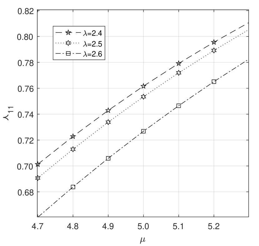
Figure 2: Mean number of server is on vacation vs $\lambda$ and $\mu$

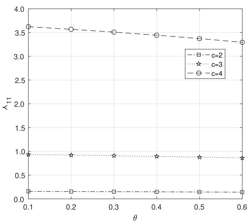
Figure 3: Mean number of server is on vacation vs $c$ and $\theta$

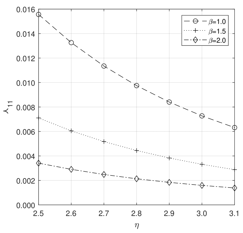
Figure 4: Mean number of server is on vacation vs $\beta$ and $\eta$

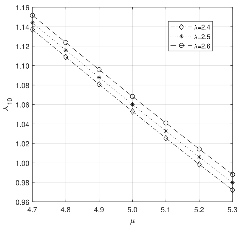
Figure 5: Mean number of busy servers vs $\lambda$ and $\mu$

Figure 6: Mean number of busy servers vs $c$ and $\theta$

Figure 7: Mean number of busy servers vs $\beta$ and $\eta$

Table 2: Expected customer lost rate with the variation of parameters

$c$	$\eta$	$\theta$	$\beta$	$\lambda$	2.4			2.5			2.6
				$\mu$	4.9	5	5.1	4.9	5	5.1	4.9	5	5.1
2	2.6	0.6	1	0.335937		0.335762	0.335567	0.344799	0.344599	0.344377	0.353376	0.353149	0.352898
			1.5	0.299024		0.298380	0.297654	0.306945	0.306244	0.305457	0.314594	0.313834	0.312982
			2	0.258399		0.256290	0.253947	0.265413	0.263225	0.260797	0.272160	0.269886	0.267368
		0.7	1	0.363575		0.363396	0.363198	0.373551	0.373347	0.373121	0.383228	0.382997	0.382740
			1.5	0.326191		0.325532	0.324791	0.335141	0.334424	0.333620	0.343806	0.343027	0.342155
			2	0.284384		0.282202	0.279775	0.292336	0.290069	0.287551	0.300004	0.297646	0.295034
		0.8	1	0.387481		0.387300	0.387099	0.398468	0.398262	0.398033	0.409148	0.408914	0.408654
			1.5	0.350030		0.349364	0.348614	0.359925	0.359200	0.358385	0.369524	0.368735	0.367851
			2	0.307557		0.305326	0.302844	0.316376	0.314056	0.311479	0.324899	0.322485	0.319808
	2.7	0.6	1	0.335617		0.335438	0.335239	0.344454	0.344250	0.344023	0.353007	0.352775	0.352518
			1.5	0.298611		0.297963	0.297234	0.306514	0.305810	0.305020	0.314147	0.313384	0.312529
			2	0.258283		0.256188	0.253860	0.265310	0.263136	0.260724	0.272069	0.269811	0.267311
		0.7	1	0.363248		0.363065	0.362862	0.373197	0.372988	0.372757	0.382848	0.382611	0.382349
			1.5	0.325758		0.325095	0.324350	0.334688	0.333968	0.333159	0.343334	0.342552	0.341676
			2	0.284249		0.282080	0.279668	0.292211	0.289958	0.287457	0.299890	0.297548	0.294953
		0.8	1	0.387150		0.386964	0.386759	0.398109	0.397898	0.397664	0.408761	0.408520	0.408255
			1.5	0.349584		0.348913	0.348159	0.359457	0.358726	0.357907	0.369035	0.368241	0.367352
			2	0.307403		0.305185	0.302718	0.316231	0.313925	0.311365	0.324765	0.322366	0.319706
	2.8	0.6	1	0.335267		0.335084	0.334880	0.344079	0.343870	0.343638	0.352606	0.352369	0.352107
			1.5	0.298189		0.297538	0.296807	0.306077	0.305371	0.304578	0.313697	0.312932	0.312074
			2	0.258254		0.256174	0.253864	0.265297	0.263139	0.260746	0.272074	0.269833	0.267352
		0.7	1	0.362890		0.362702	0.362494	0.372811	0.372597	0.372361	0.382434	0.382192	0.381924
			1.5	0.325316		0.324650	0.323901	0.334228	0.333505	0.332693	0.342858	0.342073	0.341193
			2	0.284201		0.282047	0.279653	0.292179	0.289942	0.287460	0.299875	0.297550	0.294975
		0.8	1	0.386787		0.386597	0.386386	0.397718	0.397500	0.397260	0.408339	0.408093	0.407821
			1.5	0.349127		0.348452	0.347694	0.358980	0.358245	0.357422	0.368539	0.367741	0.366849
			2	0.307338		0.305136	0.302686	0.316181	0.313891	0.311349	0.324730	0.322348	0.319708
3	2.6	0.6	1	0.332930		0.332456	0.331920	0.341724	0.341215	0.340640	0.350239	0.349693	0.349075
			1.5	0.273222		0.270263	0.267035	0.281525	0.278552	0.275309	0.289485	0.286488	0.283222
			2	0.179395		0.175302	0.171378	0.188562	0.184350	0.180292	0.197369	0.193061	0.188895
		0.7	1	0.360607		0.360135	0.359600	0.370523	0.370015	0.369441	0.380147	0.379601	0.378985
			1.5	0.299928		0.296893	0.293578	0.309259	0.306207	0.302875	0.318232	0.315155	0.311796
			2	0.201095		0.196677	0.192429	0.211321	0.206778	0.202389	0.221161	0.216517	0.212013
		0.8	1	0.384578		0.384110	0.383582	0.395513	0.395010	0.394442	0.406149	0.405608	0.404997
			1.5	0.323613		0.320538	0.317173	0.333882	0.330788	0.327405	0.343785	0.340663	0.337251
			2	0.221106		0.216424	0.211909	0.232292	0.227480	0.222818	0.243070	0.238154	0.233373
	2.7	0.6	1	0.332630		0.332159	0.331626	0.341416	0.340910	0.340338	0.349924	0.349380	0.348766
			1.5	0.273326		0.270412	0.267231	0.281644	0.278717	0.275521	0.289622	0.286671	0.283453
			2	0.181172		0.177029	0.173042	0.190381	0.186123	0.182006	0.199222	0.194872	0.190652
		0.7	1	0.360304		0.359834	0.359302	0.370210	0.369705	0.369134	0.379826	0.379283	0.378670
			1.5	0.300026		0.297037	0.293770	0.309371	0.306366	0.303083	0.318362	0.315332	0.312023
			2	0.203002		0.198535	0.194224	0.213270	0.208683	0.204236	0.223145	0.218462	0.213904
		0.8	1	0.384275		0.383809	0.383283	0.395199	0.394699	0.394133	0.405826	0.405288	0.404680
			1.5	0.323704		0.320676	0.317361	0.333987	0.330941	0.327608	0.343907	0.340833	0.337473
			2	0.223118		0.218388	0.213810	0.234346	0.229492	0.224773	0.245159	0.240206	0.235373
	2.8	0.6	1	0.332308		0.331840	0.331309	0.341086	0.340583	0.340015	0.349589	0.349049	0.348440
			1.5	0.273513		0.270649	0.267520	0.281849	0.278971	0.275829	0.289848	0.286948	0.283783
			2	0.183259		0.179058	0.174998	0.192508	0.188197	0.184014	0.201381	0.196984	0.192701
		0.7	1	0.359978		0.359510	0.358981	0.369875	0.369373	0.368806	0.379485	0.378946	0.378337
			1.5	0.300208		0.297270	0.294057	0.309570	0.306617	0.303388	0.318582	0.315605	0.312351
			2	0.205241		0.200717	0.196333	0.215550	0.210912	0.206397	0.225457	0.220729	0.216109
		0.8	1	0.383949		0.383486	0.382962	0.394864	0.394366	0.393804	0.405483	0.404948	0.404344
			1.5	0.323880		0.320903	0.317643	0.334179	0.331185	0.327908	0.344120	0.341100	0.337795
			2	0.225477		0.220692	0.216043	0.236746	0.231844	0.227060	0.247592	0.242597	0.237704
	2.6	0.6	1	0.320328		0.318532	0.316552	0.328375	0.326491	0.324421	0.336091	0.334118	0.331956
			1.5	0.223068		0.219621	0.216334	0.231259	0.227817	0.224539	0.239121	0.235698	0.232447
			2	0.161428		0.160592	0.159993	0.169064	0.168231	0.167647	0.176679	0.175839	0.175259
		0.7	1	0.347979		0.346177	0.344190	0.357126	0.355233	0.353152	0.365929	0.363943	0.361764
			1.5	0.247598		0.243935	0.240431	0.256762	0.253099	0.249598	0.265575	0.261928	0.258449
			2	0.181123		0.180255	0.179642	0.188181	0.188772	0.189630	0.196671	0.197251	0.198111
		0.8	1	0.372035		0.370244	0.368267	0.382189	0.380305	0.378231	0.391989	0.390009	0.387835
			1.5	0.269806		0.265980	0.262309	0.279859	0.276029	0.272357	0.289546	0.285727	0.282073
			2	0.199429		0.198538	0.197916	0.208741	0.207864	0.207271	0.218020	0.217147	0.216570
		0.6	1	0.320193		0.318406	0.316437	0.328241	0.326367	0.324309	0.335961	0.333998	0.331848
			1.5	0.223416		0.219966	0.216673	0.231620	0.228174	0.224890	0.239494	0.236069	0.232810
	2.7		2	0.161712		0.160913	0.160352	0.169367	0.168573	0.168030	0.177000	0.176199	0.175662
4		0.7	1	0.347841		0.346048	0.344070	0.356989	0.355106	0.353035	0.365794	0.363818	0.361651
			1.5	0.247962		0.244297	0.240787	0.257140	0.253475	0.249968	0.265967	0.262317	0.258832
			2	0.181433		0.180605	0.180035	0.189962	0.189145	0.188599	0.198462	0.197645	0.197112
		0.8	1	0.371895		0.370113	0.368146	0.382049	0.380175	0.378112	0.391851	0.389882	0.387719
			1.5	0.270182		0.266355	0.262679	0.280249	0.276418	0.272741	0.289951	0.286130	0.282470
			2	0.199762		0.198913	0.198337	0.209096	0.208264	0.207719	0.218396	0.217569	0.217043
	2.8	0.6	1	0.320052		0.318275	0.316317	0.328103	0.326240	0.324193	0.335827	0.333876	0.331739
			1.5	0.223844		0.220389	0.217087	0.232063	0.228612	0.225319	0.239952	0.236520	0.233252
			2	0.162054		0.161298	0.160785	0.169730	0.168982	0.168489	0.177382	0.176630	0.176144
		0.7	1	0.347695		0.345913	0.343946	0.356846	0.354974	0.352915	0.365655	0.363691	0.361538
			1.5	0.248412		0.244743	0.241224	0.257605	0.253936	0.250421	0.266447	0.262793	0.259298
			2	0.181807		0.181027	0.180508	0.190359	0.189592	0.189101	0.198880	0.198115	0.197638
		0.8	1	0.371748		0.369976	0.368020	0.381904	0.380041	0.377989	0.391709	0.389752	0.387602
			1.5	0.270647		0.266817	0.263133	0.280730	0.276895	0.273211	0.290447	0.286623	0.282954
			2	0.200162		0.199364	0.198844	0.209522	0.208743	0.208257	0.218845	0.218073	0.217607

Table 3: Fraction of successful rate of retrial under the parameter variation

$c$	$\eta$	$\theta$	$\beta$	$\lambda$	2.4			2.5			2.6
				$\mu$	4.9	5	5.1	4.9	5	5.1	4.9	5	5.1
2	2.6	0.6	1	98.7165		104.3344	110.0737	80.4930	84.9905	89.5778	66.1961	69.8320	73.5351
			1.5	127.8396		136.9741	146.5567	105.6185	113.1000	120.9419	87.9277	94.1030	100.5702
			2	132.6868		142.4772	152.7901	110.0718	118.1507	126.6569	92.0150	98.7337	105.8046
		0.7	1	98.6237		104.2369	109.9712	80.4062	84.8996	89.4825	66.1147	69.7470	73.4462
			1.5	127.7995		136.9321	146.5129	105.5787	113.0585	120.8986	87.8885	94.0621	100.5276
			2	132.6664		142.4565	152.7690	110.0509	118.1294	126.6352	91.9936	98.7120	105.7825
		0.8	1	98.5413		104.1504	109.8803	80.3290	84.8188	89.3979	66.0422	69.6713	73.3671
			1.5	127.7622		136.8933	146.4724	105.5418	113.0200	120.8586	87.8520	94.0241	100.4881
			2	132.6466		142.4364	152.7485	110.0306	118.1088	126.6142	91.9729	98.6909	105.7610
	2.7	0.6	1	98.8929		104.5305	110.2910	80.6439	85.1579	89.7630	66.3256	69.9755	73.6934
			1.5	127.9207		137.0666	146.6620	105.6925	113.1843	121.0378	87.9952	94.1798	100.6575
			2	132.7138		142.5082	152.8255	110.0974	118.1801	126.6905	92.0392	98.7615	105.8364
		0.7	1	98.7999		104.4328	110.1883	80.5569	85.0668	89.6675	66.2440	69.8902	73.6043
			1.5	127.8807		137.0248	146.6184	105.6529	113.1430	120.9947	87.9561	94.1391	100.6151
			2	132.6936		142.4877	152.8047	110.0767	118.1590	126.6691	92.0180	98.7400	105.8145
		0.8	1	98.7173		104.3461	110.0972	80.4795	84.9858	89.5826	66.1713	69.8143	73.5250
			1.5	127.8436		136.9861	146.5780	105.6161	113.1047	120.9548	87.9197	94.1013	100.5757
			2	132.6739		142.4678	152.7845	110.0565	118.1386	126.6483	91.9975	98.7191	105.7933
	2.8	0.6	1	99.0496		104.7049	110.4842	80.7782	85.3070	89.9278	66.4410	70.1033	73.8345
			1.5	127.9926		137.1487	146.7554	105.7583	113.2593	121.1231	88.0553	94.2482	100.7352
			2	132.7377		142.5356	152.8569	110.1201	118.2062	126.7204	92.0608	98.7862	105.8647
		0.7	1	98.9564		104.6069	110.3812	80.6910	85.2156	89.8321	66.3592	70.0178	73.7452
			1.5	127.9528		137.1071	146.7120	105.7188	113.2181	121.0801	88.0163	94.2076	100.6928
			2	132.7176		142.5153	152.8363	110.0995	118.1852	126.6991	92.0397	98.7649	105.8429
		0.8	1	98.8737		104.5200	110.2899	80.6134	85.1344	89.7470	66.2863	69.9417	73.6657
			1.5	127.9158		137.0685	146.6718	105.6821	113.1799	121.0403	87.9800	94.1698	100.6536
			2	132.6981		142.4955	152.8163	110.0795	118.1650	126.6785	92.0193	98.7442	105.8219
3	2.6	0.6	1	110.7908		113.2895	115.6987	90.7908	92.8020	94.7401	75.1104	76.7477	78.3247
			1.5	263.7748		276.9133	290.1810	215.7643	226.2968	236.9174	178.0352	186.5601	195.1446
			2	296.3682		317.9867	340.7382	245.6361	263.4209	282.1268	205.1552	219.8972	235.3933
		0.7	1	110.7415		113.2370	115.6429	90.7433	92.7517	94.6870	75.0643	76.6993	78.2739
			1.5	263.7527		276.8908	290.1578	215.7398	226.2718	236.8918	178.0087	186.5331	195.1171
			2	296.3360		317.9526	340.7023	245.6035	263.3866	282.0907	205.1224	219.8628	235.3572
		0.8	1	110.7073		113.2002	115.6034	90.7094	92.7157	94.6488	75.0307	76.6638	78.2365
			1.5	263.7358		276.8739	290.1407	215.7205	226.2525	236.8723	177.9874	186.5116	195.0954
			2	296.3050		317.9200	340.6679	245.5724	263.3539	282.0564	205.0912	219.8300	235.3228
	2.7	0.6	1	110.9687		113.4679	115.8771	90.9595	92.9722	94.9114	75.2682	76.9076	78.4864
			1.5	264.3976		277.5859	290.9050	216.3147	226.8910	237.5570	178.5220	187.0855	195.7100
			2	296.5474		318.1907	340.9698	245.8063	263.6144	282.3463	205.3163	220.0802	235.6008
		0.7	1	110.9169		113.4127	115.8184	90.9099	92.9198	94.8561	75.2203	76.8573	78.4337
			1.5	264.3798		277.5678	290.8864	216.2940	226.8700	237.5355	178.4991	187.0621	195.6861
			2	296.5168		318.1583	340.9358	245.7752	263.5817	282.3120	205.2849	220.0473	235.5662
			1	110.8805		113.3737	115.7767	90.8744	92.8820	94.8159	75.1853	76.8203	78.3947
		0.8	1.5	264.3672		277.5553	290.8739	216.2787	226.8547	237.5200	178.4813	187.0443	195.6681
			2	296.4874		318.1274	340.9032	245.7455	263.5505	282.2793	205.2550	220.0160	235.5335
	2.8	0.6	1	111.1049		113.6027	116.0101	91.0928	93.1055	95.0443	75.3956	77.0359	78.6152
			1.5	264.9401		278.1705	291.5330	216.7961	227.4098	238.1142	178.9495	187.5460	196.2047
			2	296.7068		318.3721	341.1759	245.9579	263.7868	282.5420	205.4601	220.2436	235.7859
		0.7	1	111.0504		113.5448	115.9486	91.0410	93.0507	94.9865	75.3459	76.9836	78.5604
			1.5	264.9254		278.1555	291.5175	216.7783	227.3916	238.0956	178.9290	187.5252	196.1834
			2	296.6775		318.3412	341.1434	245.9280	263.7554	282.5090	205.4298	220.2119	235.7527
		0.8	1	111.0119		113.5034	115.9044	91.0036	93.0109	94.9443	75.3092	76.9450	78.5197
			1.5	264.9161		278.1463	291.5083	216.7658	227.3792	238.0831	178.9139	187.5101	196.1681
			2	296.6494		318.3117	341.1124	245.8995	263.7255	282.4777	205.4010	220.1817	235.7212
4	2.6	0.6	1	177.8154		185.9085	194.0108	143.5752	149.9233	156.2662	117.0305	122.0666	127.0899
			1.5	276.6210		295.5775	315.3668	227.5709	242.9492	258.9817	188.6526	201.2228	214.3101
			2	349.0936		371.7439	395.2441	287.6770	306.0949	325.1817	238.9754	254.0753	269.7057
		0.7	1	177.6689		185.7526	193.8450	143.4428	149.7829	156.1175	116.9103	121.9395	126.9557
			1.5	276.5632		295.5169	315.3033	227.5143	242.8900	258.9196	188.5972	201.1649	214.2495
			2	349.0063		371.6534	395.1502	287.5963	306.0114	325.0953	238.9005	253.9977	269.6256
		0.8	1	177.5413		185.6169	193.7008	143.3275	149.6606	155.9880	116.8054	121.8288	126.8389
			1.5	276.5110		295.4622	315.2460	227.4630	242.8364	258.8636	188.5470	201.1126	214.1948
			2	348.9226		371.5665	395.0602	287.5192	305.9315	325.0125	238.8290	253.9237	269.5491
	2.7	0.6	1	178.5603		186.7159	194.8829	144.2022	150.6012	156.9967	117.5606	122.6385	127.7048
			1.5	277.1124		296.1334	315.9942	228.0172	243.4533	259.5495	189.0573	201.6791	214.8232
			2	349.6335		372.3436	395.9085	288.1600	306.6313	325.7758	239.4081	254.5555	270.2374
		0.7	1	178.4128		186.5588	194.7158	144.0689	150.4597	156.8468	117.4395	122.5105	127.5696
			1.5	277.0554		296.0737	315.9316	227.9612	243.3948	259.4882	189.0026	201.6219	214.7634
			2	349.5612		372.2691	395.8316	288.0925	306.5617	325.7041	239.3447	254.4902	270.1702
		0.8	1	178.2843		186.4221	194.5704	143.9527	150.3365	156.7163	117.3339	122.3989	127.4518
			1.5	277.0040		296.0199	315.8752	227.9107	243.3420	259.4330	188.9530	201.5702	214.7094
			2	349.4919		372.1975	395.7578	288.0280	306.4952	325.6356	239.2842	254.4279	270.1062
	2.8	0.6	1	179.2280		187.4396	195.6646	144.7650	151.2098	157.6525	118.0372	123.1526	128.2576
			1.5	277.5513		296.6299	316.5545	228.4163	243.9041	260.0573	189.4198	202.0878	215.2828
			2	350.1123		372.8750	396.4968	288.5893	307.1075	326.3029	239.7934	254.9828	270.7102
		0.7	1	179.0795		187.2814	195.4963	144.6308	151.0673	157.5015	117.9152	123.0237	128.1214
			1.5	277.4949		296.5709	316.4926	228.3609	243.8461	259.9967	189.3655	202.0311	215.2235
			2	350.0523		372.8134	396.4337	288.5325	307.0494	326.2433	239.7394	254.9275	270.6536
		0.8	1	178.9502		187.1437	195.3499	144.5138	150.9432	157.3700	117.8088	122.9112	128.0027
			1.5	277.4441		296.5177	316.4369	228.3109	243.7940	259.9421	189.3165	201.9800	215.1702
			2	349.9948		372.7544	396.3732	288.4783	306.9938	326.1865	239.6880	254.8750	270.5999

Example 4.

Table LABEL:tab3 explains the fraction of the successful rate of retrial under the parameter variation.

1. As the rate $\lambda$ increases, the fraction of the successful rate of retrial decreases due to the overflow in the waiting hall.

2. If $\mu$ increases, the number of customers in the waiting hall starts decreasing, and so a fraction of successful retrials increases. Similarly, the increase in the number of servers in the system causes an increase in the successful rate of retrials in the system.

3. As we predicted, the rate $\theta$ reduces the fraction of successful retrials when it increases because more customers from the orbit enter the waiting hall.

4. When $\beta$ increases, the inventory storage system maintains a positive stock level so that an arriving customer can purchase the item and leave the system without delay. Hence, it increases the fraction of the successful retrial rate.

5. Suppose the server returns from vacation sooner than expected, then many customers get their service without a server delay. On the other hand, if the server is on vacation, a customer has to wait some time until his turn occurs. So, if the servers are already available in the system, his turn occurs quickly. Therefore, the vacation completion rate increases the fraction of the success rate of a retrial if it increases.

Insights: When we approach a business economically, caring for the orbital customer’s arrival will influence the growth of the business. So, this example explores the characteristics of the fraction of successful retrial rates of orbit customers with parameter variation. In such a way, the parameters $c$, $\beta$, and $\eta$ have great importance to overcome the loss of retrial customers.

Example 5.

This example examines the orbit and waiting hall customer’s waiting times in Tables LABEL:tab4 and LABEL:tab5 respectively, using the parameters $\lambda,\mu,\theta,\beta,c$, and $\eta$.

1. The parameters $\mu$ and $c$ have an equivalent impact on reducing the waiting time of a customer, whether they are in the queue or in the orbit. In other words, decreasing the average time it takes to complete a service or increasing the number of servers will result in a decrease in the number of customers waiting in the queue, which will also lead to a reduction in the number of customers in orbit. This ultimately leads to a reduction in the waiting time for both sets of customers.

2. In a similar way, the replenishment rate helps the system avoid a shortage of inventory if it increases. Since the inventory is positive, the customers in the waiting hall do not need to wait a long time in the queue due to the lack of inventory. So, both customers’ waiting times will be reduced.

3. The vacation completion rate also contributes to reducing the waiting time of the customers in a queue or orbit. This rate ensures that the servers are mostly available when it increases.

4. If $\lambda$ increases, the number of customers in the waiting hall increases and soon overflows. Thus, both customers’ waiting times in the queue and the orbit increase whenever it increases.

5. Increasing $\theta$ only affects the waiting time of customers in the orbit, not those in the waiting hall. This is because the waiting hall quickly fills up, and an increase in $\theta$ results in a decrease in the number of customers in orbit, which ultimately leads to a reduction in their waiting time.

Insights: It is crucial to analyze waiting time in customer-centric service systems in order to run a successful business. Ensuring customer satisfaction through the service system is paramount in this environment, as reducing customers’ waiting time leads to higher levels of satisfaction and a better reputation for the company. This, in turn, leads to more customers returning to make additional purchases within the same system. Therefore, this example serves as a persuasive argument for readers and business people to prioritize reducing waiting times for their customers.

Table 4: Mean waiting time for orbit customers under the impact of parameters

$c$	$\eta$	$\theta$	$\beta$	$\lambda$	2.4			2.5			2.6
				$\mu$	4.9	5	5.1	4.9	5	5.1	4.9	5	5.1
2	2.6	0.6	1	0.033279		0.031156	0.029165	0.038288	0.035851	0.033563	0.043807	0.041027	0.038417
			1.5	0.025736		0.023661	0.021773	0.029994	0.027609	0.025436	0.034780	0.032052	0.029563
			2	0.022679		0.021326	0.020101	0.027110	0.025514	0.024070	0.032177	0.030308	0.028615
		0.7	1	0.025422		0.023791	0.022263	0.029257	0.027384	0.025628	0.033485	0.031347	0.029342
			1.5	0.019850		0.018261	0.016815	0.023129	0.021302	0.019638	0.026814	0.024724	0.022818
			2	0.017888		0.016829	0.017681	0.021359	0.020112	0.018982	0.025324	0.023865	0.022543
		0.8	1	0.020201		0.018899	0.017681	0.023255	0.021759	0.020358	0.026622	0.024914	0.023314
			1.5	0.015921		0.014655	0.013503	0.018548	0.017092	0.015766	0.021498	0.019833	0.018314
			2	0.014636		0.013775	0.012995	0.017460	0.016447	0.015529	0.020681	0.019498	0.018125
	2.7	0.6	1	0.033226		0.031100	0.029105	0.038228	0.035786	0.033495	0.043738	0.040953	0.038339
			1.5	0.025710		0.023638	0.021753	0.029966	0.027584	0.025414	0.034749	0.032024	0.029540
			2	0.022724		0.021370	0.020145	0.027164	0.025568	0.024124	0.032243	0.030374	0.028681
		0.7	1	0.025383		0.023749	0.022219	0.029212	0.027336	0.025577	0.033433	0.031292	0.029284
			1.5	0.019831		0.018244	0.016801	0.023109	0.021285	0.019623	0.026792	0.024705	0.022801
			2	0.017923		0.016863	0.015904	0.021402	0.020154	0.019024	0.025376	0.023917	0.022594
		0.8	1	0.020171		0.018867	0.017647	0.023221	0.021722	0.020319	0.026582	0.024872	0.023270
			1.5	0.015907		0.014643	0.013493	0.018534	0.017079	0.015755	0.021483	0.019819	0.018303
			2	0.014664		0.013803	0.013022	0.017494	0.016481	0.015563	0.020723	0.019540	0.018466
	2.8	0.6	1	0.033163		0.031032	0.029033	0.038154	0.035708	0.033412	0.043655	0.040865	0.038245
			1.5	0.025677		0.023609	0.021727	0.029930	0.027551	0.025385	0.034709	0.031989	0.029509
			2	0.022773		0.021419	0.020193	0.027224	0.025628	0.024184	0.032316	0.030447	0.028753
		0.7	1	0.025335		0.023699	0.022166	0.029158	0.027278	0.025516	0.033371	0.031226	0.029215
			1.5	0.019808		0.018223	0.016782	0.023084	0.021262	0.019603	0.026764	0.024680	0.022780
			2	0.017961		0.016901	0.015941	0.029158	0.020202	0.019071	0.025433	0.023974	0.022651
		0.8	1	0.020135		0.018829	0.017606	0.023179	0.021678	0.020272	0.026535	0.024821	0.023216
			1.5	0.015890		0.014627	0.013479	0.018515	0.017063	0.015741	0.021462	0.019801	0.018287
			2	0.014695		0.013834	0.013053	0.017532	0.016520	0.015601	0.020770	0.019586	0.018513
			1	0.019171		0.018738	0.018339	0.022778	0.022271	0.021805	0.026844	0.026255	0.025712
		0.6	1.5	0.009109		0.008656	0.008243	0.010849	0.010318	0.009833	0.012827	0.012209	0.011644
			2	0.008052		0.007493	0.006991	0.009511	0.008858	0.008271	0.011164	0.010405	0.009722
	2.6	0.7	1	0.015182		0.014840	0.014525	0.018019	0.017620	0.017252	0.021215	0.020751	0.020323
			1.5	0.007154		0.006800	0.006476	0.008513	0.008097	0.007718	0.010056	0.009573	0.009131
			2	0.006266		0.005835	0.005446	0.007396	0.006892	0.006438	0.008674	0.008089	0.007561
3		0.8	1	0.012463		0.012183	0.011925	0.014779	0.014452	0.014151	0.017384	0.017005	0.016655
			1.5	0.005831		0.005543	0.005280	0.006933	0.006595	0.006287	0.008183	0.007791	0.007433
			2	0.005066		0.004720	0.004407	0.005976	0.005571	0.005206	0.007004	0.006534	0.006111
	2.7	0.6	1	0.019119		0.018689	0.018292	0.022710	0.022206	0.021742	0.026756	0.026170	0.025630
			1.5	0.009075		0.008623	0.008211	0.010805	0.010276	0.009793	0.012774	0.012157	0.011594
			2	0.008039		0.007481	0.006979	0.009496	0.008843	0.008255	0.011145	0.010386	0.009703
		0.7	1	0.015142		0.014802	0.014489	0.017967	0.017570	0.017203	0.021147	0.020685	0.020260
			1.5	0.007128		0.006774	0.006451	0.008479	0.008065	0.007687	0.010014	0.009532	0.009092
			2	0.006256		0.005824	0.005436	0.007383	0.006879	0.006425	0.008659	0.008073	0.007546
		0.8	1	0.012431		0.012153	0.011896	0.014737	0.014412	0.014112	0.017330	0.016953	0.016605
			1.5	0.005810		0.005522	0.005260	0.006905	0.006569	0.006262	0.008149	0.007758	0.007401
			2	0.005057		0.004711	0.004399	0.005965	0.005560	0.005196	0.006991	0.006521	0.006098
		0.6	1	0.019077		0.018649	0.018254	0.022653	0.022152	0.021689	0.026682	0.026099	0.025561
			1.5	0.009043		0.008593	0.008182	0.010766	0.010238	0.009756	0.012725	0.012110	0.011548
			2	0.008026		0.007467	0.006965	0.009479	0.008826	0.008239	0.011125	0.010366	0.009682
		0.7	1	0.015110		0.014772	0.014460	0.017924	0.017528	0.017164	0.021091	0.020631	0.020207
	2.8		1.5	0.007103		0.006751	0.006429	0.008448	0.008035	0.007658	0.009976	0.009496	0.009057
			2	0.006245		0.005813	0.005425	0.007370	0.006865	0.006412	0.008642	0.008057	0.007530
		0.8	1	0.012406		0.012128	0.011873	0.014703	0.014379	0.014080	0.017285	0.016909	0.016563
			1.5	0.005790		0.005503	0.005241	0.006881	0.006545	0.006239	0.008118	0.007729	0.007373
			2	0.005048		0.004702	0.004390	0.005953	0.005549	0.005184	0.006977	0.006507	0.006084
4	2.6	0.6	1	0.012093		0.011549	0.011053	0.014585	0.013946	0.013362	0.017449	0.016702	0.016020
			1.5	0.009639		0.008917	0.008271	0.011361	0.010523	0.009771	0.013316	0.012348	0.011479
			2	0.013761		0.012535	0.011430	0.015787	0.014394	0.013140	0.018046	0.016471	0.015052
		0.7	1	0.009572		0.009143	0.008751	0.011533	0.011030	0.010569	0.013784	0.013196	0.012659
			1.5	0.007517		0.006960	0.006460	0.008854	0.008207	0.007626	0.010371	0.009624	0.008953
			2	0.010514		0.009585	0.008748	0.012064	0.011009	0.010059	0.013793	0.012600	0.011524
		0.8	1	0.008360		0.007628	0.006968	0.009456	0.009045	0.008668	0.011292	0.010812	0.010373
			1.5	0.006090		0.005642	0.005239	0.007169	0.006649	0.006182	0.008392	0.007792	0.007253
			2	0.007855		0.007504	0.007183	0.009596	0.008764	0.008014	0.010972	0.010031	0.009182
	2.7	0.6	1	0.012031		0.011489	0.010993	0.014508	0.013870	0.013287	0.017354	0.016609	0.015927
			1.5	0.009633		0.008909	0.008260	0.011351	0.010511	0.009757	0.013303	0.012332	0.011461
			2	0.013908		0.012671	0.011554	0.015950	0.014544	0.013276	0.018226	0.016636	0.015202
		0.7	1	0.009524		0.009096	0.008704	0.011473	0.010970	0.010510	0.013710	0.013123	0.012587
			1.5	0.007511		0.006952	0.006451	0.008846	0.008197	0.007614	0.010360	0.009611	0.008938
			2	0.010621		0.009684	0.008839	0.012184	0.011119	0.010158	0.013924	0.012720	0.011633
		0.8	1	0.007816		0.007466	0.007145	0.009407	0.008996	0.008620	0.011232	0.010753	0.010315
			1.5	0.006084		0.005635	0.005232	0.007161	0.006640	0.006172	0.008382	0.007781	0.007240
			2	0.008442		0.007704	0.007037	0.009687	0.008847	0.008089	0.011072	0.010122	0.009265
	2.8	0.6	1	0.011976		0.011434	0.010939	0.014439	0.013802	0.013220	0.017269	0.016525	0.015845
			1.5	0.009625		0.008899	0.008249	0.011340	0.010497	0.009742	0.013289	0.012315	0.011442
			2	0.014036		0.012788	0.011662	0.016092	0.014675	0.013395	0.018383	0.016780	0.015332
		0.7	1	0.009481		0.009053	0.008662	0.011419	0.010917	0.010458	0.013643	0.013058	0.012522
			1.5	0.007504		0.006944	0.006441	0.008836	0.008186	0.007602	0.010348	0.009597	0.008922
			2	0.010715		0.009770	0.008917	0.012287	0.011214	0.010245	0.014039	0.012825	0.011728
		0.8	1	0.007781		0.007431	0.007111	0.009364	0.008953	0.008578	0.011178	0.010700	0.010262
			1.5	0.006078		0.005628	0.005224	0.007153	0.006631	0.006162	0.008371	0.007769	0.007227
			2	0.008514		0.007769	0.007096	0.009766	0.008919	0.008155	0.011160	0.010202	0.009337

Table 5: Mean waiting time for a waiting hall customer under the impact of parameters different parameters

$c$	$\eta$	$\theta$	$\beta$	$\lambda$	2.4			2.5			2.6
				$\mu$	4.9	5	5.1	4.9	5	5.1	4.9	5	5.1
2	2.6	0.6	1	0.975550		0.972322	0.969182	1.017790	1.014531	1.011356	1.063851	1.060560	1.057346
			1.5	0.918359		0.913785	0.909720	0.954241	0.949683	0.945658	0.993067	0.988520	0.984533
			2	0.898471		0.889304	0.880625	0.931381	0.921842	0.912809	0.966996	0.957039	0.947606
		0.7	1	1.031784		1.028592	1.025490	1.076556	1.073328	1.070184	1.125348	1.122080	1.118891
			1.5	0.979389		0.974836	0.970790	1.018319	1.013766	1.009745	1.060450	1.055891	1.051891
			2	0.961433		0.952232	0.943521	0.997523	0.987934	0.978854	1.036583	1.026558	1.017060
		0.8	1	1.079977		1.076826	1.073767	1.126822	1.123629	1.120524	1.177840	1.174602	1.171448
			1.5	1.033017		1.028464	1.024417	1.074575	1.070005	1.065964	1.119558	1.114962	1.110923
			2	1.017699		1.008509	0.999808	1.056616	1.047028	1.037947	1.098742	1.088706	1.079195
	2.7	0.6	1	0.977509		0.974334	0.971245	1.019765	1.016559	1.013433	1.065839	1.062599	1.059433
			1.5	0.921317		0.916985	0.913159	0.957328	0.953022	0.949246	0.996280	0.991996	0.988269
			2	0.900097		0.891166	0.882744	0.933045	0.923748	0.914981	0.968686	0.958977	0.949817
		0.7	1	1.034013		1.030884	1.027843	1.078810	1.075643	1.072559	1.127622	1.124414	1.121284
			1.5	0.982719		0.978440	0.974667	1.021795	1.017528	1.013790	1.064069	1.059808	1.056103
			2	0.963270		0.954336	0.945917	0.999401	0.990087	0.981308	1.038490	1.028746	1.019557
		0.8	1	1.082456		1.079377	1.076387	1.129332	1.126210	1.123173	1.180377	1.177208	1.174121
			1.5	1.036694		1.032446	1.028701	1.078413	1.074160	1.070435	1.123554	1.119289	1.115578
			2	1.019733		1.010839	1.002462	1.058695	1.049411	1.040663	1.100852	1.091127	1.081957
	2.8	0.6	1	0.976429		0.973224	0.970107	1.018673	1.015438	1.012285	1.064737	1.061469	1.058277
			1.5	0.919694		0.915229	0.911273	0.955631	0.951187	0.947274	0.994511	0.990082	0.986213
			2	0.899205		0.890144	0.881582	0.932130	0.922701	0.913788	0.967756	0.957910	0.948601
		0.7	1	1.032785		1.029621	1.026546	1.077566	1.074365	1.071248	1.126364	1.123122	1.119960
			1.5	0.980892		0.976463	0.972541	1.019885	1.015461	1.011568	1.062077	1.057652	1.053785
			2	0.962262		0.953181	0.944603	0.998368	0.988904	0.979960	1.037439	1.027542	1.018183
		0.8	1	1.081092		1.077973	1.074946	1.127948	1.124787	1.121713	1.178975	1.175768	1.172644
			1.5	1.034677		1.030262	1.026352	1.076304	1.071878	1.067980	1.121355	1.116908	1.113017
			2	1.018616		1.009560	1.001006	1.057552	1.048101	1.039171	1.099690	1.089794	1.080437
3	2.6	0.6	1	0.964554		0.961434	0.958382	1.006429	1.003233	1.000110	1.052077	1.048801	1.045599
			1.5	0.919601		0.918128	0.916615	0.957597	0.956216	0.954781	0.998763	0.997500	0.996168
			2	0.849779		0.848698	0.848103	0.879957	0.878935	0.878442	0.912101	0.911111	0.910702
		0.7	1	1.019668		1.016667	1.013731	1.064013	1.060936	1.057926	1.112328	1.109169	1.106081
			1.5	0.979121		0.977769	0.976373	1.019974	1.018709	1.017386	1.064226	1.063073	1.061847
			2	0.911064		0.910350	0.910125	0.944185	0.943540	0.943427	0.979490	0.978884	0.978864
		0.8	1	1.067031		1.064151	1.061333	1.113404	1.110449	1.107558	1.163900	1.160865	1.157895
			1.5	1.031099		1.029849	1.028553	1.074354	1.073184	1.071957	1.121199	1.120133	1.118995
			2	0.965981		0.965578	0.965661	1.001729	1.001398	1.001600	1.039859	1.039572	1.039874
	2.7	0.6	1	0.966382		0.963284	0.960255	1.008266	1.005092	1.001990	1.053920	1.050665	1.047484
			1.5	0.923920		0.922543	0.921121	0.962104	0.960821	0.959479	1.003467	1.002306	1.001067
			2	0.855614		0.854943	0.854746	0.886073	0.885492	0.885428	0.918491	0.917976	0.918029
		0.7	1	1.021742		1.018769	1.015859	1.066102	1.063052	1.060068	1.114428	1.111296	1.108233
			1.5	0.983965		0.982728	0.981440	1.025034	1.023887	1.022674	1.069512	1.068481	1.067369
			2	0.917581		0.917327	0.917547	0.951017	0.950864	0.951231	0.986627	0.986552	0.987050
		0.8	1	1.069330		1.066482	1.063695	1.115723	1.112799	1.109937	1.166235	1.163230	1.160290
			1.5	1.036431		1.035314	1.034143	1.079928	1.078894	1.077794	1.127025	1.126100	1.125094
			2	0.973803		0.973229	0.973128	1.010161	1.009430	1.009219	1.048852	1.047981	1.047684
	2.8	0.6	1	0.963059		0.959919	0.956850	1.004934	1.001719	0.998578	1.050585	1.047290	1.044070
			1.5	0.916002		0.914447	0.912859	0.953856	0.952393	0.950882	0.994875	0.993529	0.992119
			2	0.844838		0.843401	0.842462	0.874797	0.873395	0.872533	0.906732	0.905335	0.904528
		0.7	1	1.017965		1.014941	1.011983	1.062307	1.059207	1.056176	1.110620	1.107439	1.104330
			1.5	0.975079		0.973630	0.972144	1.015769	1.014405	1.012990	1.059850	1.058597	1.057278
			2	0.905546		0.904435	0.903824	0.938423	0.937353	0.936826	0.973494	0.972433	0.971968
		0.8	1	1.065139		1.062232	1.054388	1.111505	1.108523	1.105607	1.161997	1.158935	1.155942
			1.5	1.026645		1.025283	1.023884	1.069717	1.068433	1.067099	1.116371	1.115189	1.113942
			2	0.959931		0.959091	0.958749	0.995412	0.994613	0.994359	1.033287	1.032499	1.032311
4	2.6	0.6	1	0.963062		0.959906	0.956833	1.004897	1.001674	0.998538	1.050476	1.047182	1.043978
			1.5	0.924775		0.921845	0.918965	0.963796	0.960777	0.957810	1.006243	1.003127	1.000066
			2	0.886673		0.884925	0.883131	0.923039	0.921270	0.919446	0.962503	0.960714	0.958861
		0.7	1	1.016781		1.013786	1.010869	1.061020	1.057959	1.054978	1.109193	1.106060	1.103011
			1.5	0.979942		0.977146	0.974397	1.021569	1.018682	1.015845	1.066836	1.063851	1.060918
			2	0.943481		0.941859	0.940187	0.982624	0.980978	0.979274	1.025091	1.023424	1.021687
		0.8	1	1.062728		1.059883	1.057110	1.108945	1.106034	1.103198	1.159246	1.156265	1.153361
			1.5	1.027726		1.025060	1.022438	1.071528	1.068772	1.066061	1.119142	1.116289	1.113483
			2	0.993303		0.991796	0.990237	1.034798	1.033265	1.031671	1.079803	1.078246	1.076619
			1	0.964210		0.961075	0.958024	1.006057	1.002855	0.999739	1.051645	1.048372	1.045187
		0.6	1.5	0.926877		0.923998	0.921168	0.965947	0.962980	0.960062	1.008438	1.005374	1.002363
			2	0.890140		0.888498	0.886807	0.926634	0.924974	0.923255	0.966221	0.964543	0.962797
		0.7	1	1.017997		1.015026	1.012132	1.062248	1.059210	1.056252	1.110428	1.107319	1.104292
	2.7		1.5	0.982190		0.979451	0.976757	1.023869	1.021040	1.018257	1.069182	1.066255	1.063378
			2	0.947227		0.945722	0.944163	0.986510	0.984984	0.983395	1.029113	1.027568	1.025950
		0.8	1	1.064001		1.061182	1.058435	1.110229	1.107344	1.104533	1.160536	1.157581	1.154702
			1.5	1.030112		1.027508	1.024944	1.073968	1.071274	1.068623	1.121631	1.118840	1.116095
			2	0.997319		0.995938	0.994502	1.038966	1.037563	1.036096	1.084120	1.082695	1.081197
	2.8	0.6	1	0.965554		0.962445	0.959417	1.007420	1.004243	1.001150	1.053022	1.049773	1.046612
			1.5	0.929374		0.926555	0.923781	0.968514	0.965606	0.962747	1.011069	1.008066	1.005113
			2	0.894262		0.892743	0.891171	0.930930	0.929396	0.927799	0.970687	0.969140	0.967520
		0.7	1	1.019425		1.016482	1.013615	1.063694	1.060683	1.057752	1.111887	1.108805	1.105805
			1.5	0.984870		0.982197	0.979566	1.026622	1.023860	1.021142	1.072003	1.069144	1.066331
			2	0.951692		0.950323	0.948896	0.991165	0.989779	0.988327	1.033956	1.032554	1.031076
		0.8	1	1.065501		1.062713	1.059994	1.111746	1.108891	1.106109	1.162066	1.159140	1.156289
			1.5	1.032963		1.030430	1.027936	1.076897	1.074275	1.071694	1.124632	1.121914	1.119239
			2	1.002114		1.000883	0.999590	1.043969	1.042718	1.041399	1.089327	1.088060	1.086713

Example 6.

This example explores different performance measures for the parameters $N$ and $S$.

1. Figure 11 shows that increasing the size of the waiting hall would increase the $ETC$. Because $\curlywedge_{6}$ increases when $N$ increases. While varying the maximum inventory level $S$, a local minimum is obtained.

2. By increasing the waiting hall size, $\curlywedge_{6}$ experiences an increase. Additionally, Figure 11 shows the optimum mean waiting time for customers in the waiting hall, which is determined by varying the maximum inventory level.

3. Figure 11 shows that increasing the values of $S$ and $N$, decreases the mean waiting time of the customer in orbit. Because orbit customers can enter the waiting hall as its size increases. Similarly, when $S$ is increasing, customers in the waiting hall get service and leave quickly, which gives orbital customers a chance to enter the waiting hall.

4. As the number of customers in the waiting hall and items in the inventory increase, the possibility that a server goes on vacation is reduced, which is clear from Figure 11.

5. From Figure 12, we see that increasing the waiting hall size reduces customer loss. When $N=5,10$ the expected customer loss ratio is small, whereas when we choose a large $N$, the expected customer loss ratio is high. Similarly, if the product availability increases, the customer in the waiting hall can get their service as much as possible and leaves the system soon. If a new customer faces that a waiting hall is full, his loss rate is to be controlled.

Insights: When there is a large waiting room, the number of sales goes up because customers are less likely to leave, and the average time customers wait in the orbit goes down. Also, the convexity obtained for total cost and waiting time for the waiting hall suggests that an optimal inventory can be maintained.

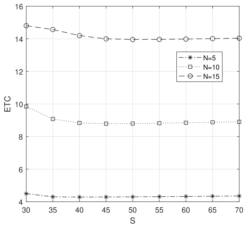
Figure 8: Expected total cost vs $N$ and $S$

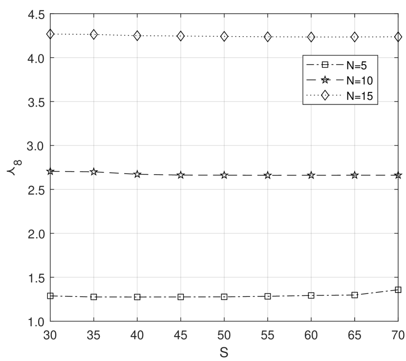
Figure 9: Mean waiting time for waiting hall vs $N$ and $S$

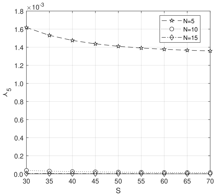
Figure 10: Mean waiting time for Orbit vs $N$ and $S$

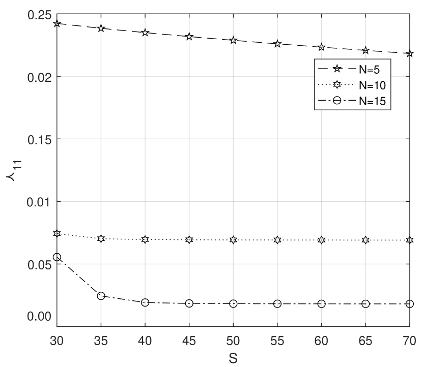
Figure 11: Mean number of server is on vacation vs $N$ and $S$

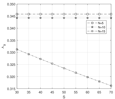
Figure 12: Mean number of customer lost vs $N$ and $S$

6 Conclusion

In this article, we investigated a multi-server queueing-inventory system with asynchronous multiple-server vacations. In addition, this model explored the retrial facility and $(s,Q)$ reordering policy for the replenishment process. As per the assumptions, a six-dimensional stochastic process is framed and transformed into an infinitesimal matrix by the transition of states. The stability condition and joint probability vector are obtained through the matrix geometric approximation method, based on the structure of the infinitesimal generator matrix. Moreover, the expected total cost function is established by considering certain system performance measures.

From the analysis of this paper, we observe the following results:

6.1 Observations

These observations are obtained by the numerical investigations:

1. From the parameter analysis, $\beta$, $\eta$, and $\mu$ are directly proportional to an expected total cost, whereas $\lambda$, $\theta$ and $c$ are inversely proportional to the expected total cost.

2. The parameters $\lambda$, $\theta$ were calculated using the mean number of busy servers with a direct variation property. On the other hand, $\beta$, $\eta$, and $\mu$ contribute to give a rest period to the servers and react with an indirect variation.

3. The expected loss rate of a customer is controlled by the increase of the parameters $\beta$, $\eta$, $c$ and $\mu$.

4. The fraction of the successful retrial rate of an orbit customer is slowed down due to the overflow of the waiting hall. To control such an overflow, one can increase the values of parameters $\beta$, $\eta$, $c$, and $\mu$ as required.

5. The waiting time of queue and orbit customers has an indirect variation relation with the parameters $\beta$, $\eta$, $c$ and $\mu$. As the situation requires, one can vary the parameter value to get the desired output.

6.2 Limitations

When we consider $c=1$, this model converts into a single server QIS with multiple server vacations. If the retrial customer is independent of the customer in the orbit, then the corresponding classical retrial policy is converted to a constant retrial policy. Assuming $p=1$, then the proposed system sends the overflowing customers to an orbit compulsorily whereas if we assume $p=0$ all the customers are considered to be lost.

6.3 Future Direction

The proposed model may be discussed with synchronous vacations among the multi-server queueing-inventory system in future research.

References

• [1] Melikov, A. Z.; Molchanov, A. A. Stock optimization in transport/storage. Cybernetics and Systems Analysis. 1992, 28, 484-487.
• [2] Sigman, K.; Simchi-Levi, D. Light traffic heuristic for an $M/G/1$ queue with limited inventory. Annals of Operations Research. 1992, 40, 371-380.
• [3] Berman, O.; Kaplan, E.H.; Shimshak, D.G. Deterministic Approximations for Inventory Management at Service Facilities. IIE Trans. 1993, 25, 98-104.
• [4] AL Maqbali, K. A. K.; Joshua, V. C.; Achyutha Krishnamoorthy. On a single server queueing inventory system. In International Conference on Distributed Computer and Communication Networks. 2020, 579-588.
• [5] Nisha Mathew; Joshua, V. C.; Krishnamoorthy, A. A Queueing Inventory System with Two Channels of Service. International Conference on Distributed Computer and Communication Networks. 2020, LNCCN, 12563, 604-616.
• [6] Krishnamoorthy, A.; Sajeev S. Nair; Viswanath C. Narayanan. An inventory model with server interruptions. In Proceedings of the $5^{th}$ International Conference on Queueing Theory and Network Applications. 2010, 132-139.
• [7] Krishnamoorthy, A.; Manikandan, R.; Lakshmy, B. A revisit to queueing-inventory system with positive service time. Annals of Operations Research. 2015, 233(1), 221-236.
• [8] Artalejo, J.R.; Krishnamoorthy, A.; Lopez-Herrero, M.J. Numerical analysis of (s, S) inventory systems with repeated attempts.Annals of Operations Research. 2006, 141, 67-83.
• [9] Manuel, P.; Sivakumar, B.; Arivarignan, G. Perishable inventory system with postponed demands and negative customers.Journal of Applied Mathematics and Decision Sciences. 2007, 94850.
• [10] Ushakumari, P.V. On (s,S)๐‘ ๐‘†(s,S) inventory system with random lead time and repeated demands. Journal of Applied Mathematics and Stochastic Analysis. 2006, 81508.
• [11] Nithya, M.; Sugapriya, C.; Selvakumar, S.; Jeganathan, K.; Harikrishnan, T. A Markovian two commodity queueing?inventory system with compliment item and classical retrial facility. Ural Mathematical Journal. 2022, 8(1), 90-116.
• [12] Daniel, J. K.; Ramanarayanan, R. An inventory system with two servers and rest periods. In Cahiers du C.E.R.O Bruxelles: University Libre De Bruxelles. 1987, 29, 95-100.
• [13] Daniel, J. K.; Ramanarayanan, R. An (s,S)๐‘ ๐‘†(s,S) inventory system with rest periods to the server. Naval Research Logistics. John Wiley and Sons. 1988, 35, 119-123.
• [14] Yuying Zhang; Dequan Yue; Wuyi Yue. A queueing-inventory system with random order size policy and server vacations. Annals of Operations Research. 2020, 310, 595-620.
• [15] Dequan Yue; Yaling Qin. A Production Inventory System with Service Time and Production Vacations. Journal of Systems Science and Systems Engineering. 2019, 28, 168-180.
• [16] Koroliuk, V. S.; Melikov, A. Z.; Ponomarenko, L. A.; Rustamov, A. M. Models of Perishable Queueing Inventory Systems with Server Vacation. Cybernetics and Systems Analysis. 2018, 54(1), 31-44.
• [17] Radhamani, V; Sivakumar, B; Arivarignan, G. A Comparative Study on Replenishment Policies for Perishable Inventory System with Service Facility and Multiple Server Vacation.OPSEARCH. 2022, 59(1), 229-265.
• [18] Ayyappan, G.; Gurulakshmi, G. A.; Somasundaram, B. Analysis of $MAP/PH/1$ Queueing model with Multiple Vacations, Optional Service, Close-down, Setup, Breakdown, Phase Type Repair and Impatient Customers. Reliability: Theory and Applications. 2022, 17(2), 447-468.
• [19] Revathi, C.; Francis Raj, L. Search of arrivals of an $M/G/1$ retrial queueing system with delayed repair and optional re-service using modified Bernoulli vacation. Journal of Computational Mathematica. 2022, 6(1), 200-209.
• [20] Yadavalli, V.S.S.; Jeganathan, K. Perishable Inventory Model with Two Heterogeneous Servers Including One with Multiple Vacations and Retrial Customers. Journal of Control and Systems Engineering. 2015, 3, 10-34.
• [21] Jeganathan, K.; Reiyas, M.A.; Lakshmi, K.P.; Saravanan, S. Two Server Markovian Inventory Systems with Server Interruptions: Heterogeneous Vs. Homogeneous Servers. Mathematics and Computers in Simulation. 2019, 155, 177-200.
• [22] Sugapriya, C.; Nithya, M.; Jeganathan, K.; Anbazhagan, N.; Joshi, Gyanendra P.; Yang Eunmok; Seo Suseok. Analysis of Stock-Dependent Arrival Process in a Retrial Stochastic Inventory System with Server Vacation. Processes. 2022, 10(1), 1-25.
• [23] Sivakumar, B. An inventory system with retrial demands and multiple server vacation. Quality Technology & Quantitative Management. 2011, 8(2), 125-146.
• [24] Krishnamoorthy A.; Manikandan R.; Dhanya Shajin. Analysis of a Multi-server Queueing-Inventory System. Advances in Operations Research. (2015), 1-16.
• [25] Yadavalli, V.S.S.; Sivakumar, B.; Arivarignan, G.; Olufemi Adetunji. A finite source multi-server inventory system with service facility. Computers & Industrial Engineering. (2012), 63(4), 739-753.
• [26] Fong-Fan Wang; Amita Bhagat; Tsan-Ming Chang. Analysis of priority multi-server retrial queueing inventory systems with MAP arrivals and exponential services. OPSEARCH, Springer; Operational Research Society of India. (2017), 54(1), 44-66.
• [27] Anoop N. Nair.; Jacob, M.J. On the distribution of an $(r,Q)$ inventory with lead time via multi-server queues. International Journal of Intelligent Enterprise. (2015), 3(1), 3-18.
• [28] Chakravarthy, S.R.; Shajin, D.; Krishnamoorthy, A. Infinite Server Queueing-Inventory Models. Journal of the Indian Society for Probability and Statistics. (2020), 21, 43-68.
• [29] Fong-Fan Wang. Approximation and Optimization of a Multi-Server Impatient Retrial Inventory-Queueing System with Two Demand Classes. Quality Technology & Quantitative Management. (2015), 12(3), 269-292.
• [30] Gabi Hanukov; Tal Avinadav; Tatyana Chernonog; Uri Yechiali. A multi-server queueing-inventory system with stock-dependent demand. IFAC-PapersOnLine. (2019), 52(13), 671-676.
• [31] Nair, A.N.; Jacob, M.J.; Krishnamoorthy, A. The multi server M/M/(s,S)๐‘€๐‘€๐‘ ๐‘†M/M/(s,S) queueing inventory system. Annals of Operations Research. (2013), 233, 321-333.
• [32] Paul, M.; Sivakumar, B.; Arivarignan, G. A Multi-Server Perishable Inventory System With Service Facility. Pacific Journal of Applied Mathematics. (2009), 2, 69-82.
• [33] Rajkumar, M.; Sivakumar, B.; Arivarignan, G. An infinite queue at a multi-server inventory system. International Journal of Inventory Research. (2014), 2, 189-221.
• [34] Rasmi, K.; Jacob, M.J. Analysis of a multiserver queueing inventory model with self-service. International Journal of Mathematical Modelling and Numerical Optimisation. (2021), 11(3), 275-291.
• [35] Jeganathan, K.; Harikrishnan, T.; Selvakumar, S.; Anbazhagan, N.; Amutha, S.; Acharya, S.; Dhakal, R.; Joshi, GP. Analysis of Interconnected Arrivals on Queueing-Inventory System with Two Multi-Server Service Channels and One Retrial Facility. Electronics. 2021, 10(5), 576.
• [36] Harikrishnan, T.; Jeganathan, K.; Selvakumar, S.; Anbazhagan, N.; Cho, W.; Joshi, G.P.; Son, K.C. Analysis of Stochastic $M/M/c/N$ Inventory System with Queue-Dependent Server Activation, Multi-Threshold Stages and Optional Retrial Facility. Mathematics, 2022, 10, 2682.
• [37] Bright, L.; Taylor, P.G. Calculating the equilibrium distribution in level-dependent quasi-birth-and-death processes. Communications in Statistics-Stochastic Models. 1995, 11(3), 497-525.
• [38] Zaiming Liu, Xuxiang Luo, Jinbiao Wu. Analysis of an M/PH/1 Retrial Queueing-Inventory System with Level Dependent Retrial Rate. Mathematical Problems in Engineering, 2020, 2020, 1-10.
• [39] Reshmi, P.S.; Jose, K.P. A MAP/PH/1 Perishable Inventory System with Dependent Retrial Loss. International Journal of Applied and Computational Mathematics, 2020, 6(153), 1-11.
• [40] Rejitha, K.R.; Jose, K.P. A stochastic inventory system with two modes of service and retrial of customers. OPSEARCH, 2018, 55, 134-149 .
• [41] Narayanan, V.C.; Deepak, T. G.; Krishnamoorthy, A.; Krishnakumar, B. On an (s,S)๐‘ ๐‘†(s,S) Inventory Policy with Service Time, Vacation to Server and Correlated Lead Time. Quality Technology & Quantitative Management, 2008, 5(2), 129-143.
• [42] Artalejo, J.R.; Pozo, M. Numerical calculation of the stationary distribution of the main multi-server retrial queue. Annals of Operations Research, 2002, 116, 41-56.
• [43] Neuts, M.F.; Rao, B.M. Numerical investigation of a multiserver retrial model. Queueing Systems, 1990, 7, 169-189.
• [44] Chakravarthy, S.R.; Krishnamoorthy, A.; Joshua, V.C. Analysis of a multi-server retrial queue with search of customers from the orbit. Performance Evaluation, 2006, 63(8), 776-798.
• [45] Neuts, M.F. Matrix-Geometric Solutions in Stochastic Modelsโ€”An Algorithmic Approach, Dover Publication Inc. 1981, New York, NY, USA.
• [46] Latouche, G.; Ramaswamy, V. Introduction to matrix analytic methods in stochastic model. ASA/SIAM Series on Statistics and Applied Probability, 1999.