Abstract

General Relativity provides us with some solutions for rotating black holes. However, there are some problems associated with them: the appearance of singularities, the possibility of violations of the cosmic censorship conjecture, the existence of regions where the mass acts repulsively and the violation of causality. Many authors consider that these problems reveal the existence of certain limits in the applicability of General Relativity. For instance, it is believed that the same existence of singularities in the classical black hole solutions is a weakness of the theory and that a full Quantum Gravity Theory would provide us with singularity-free black hole models. In this paper, the generic properties of the interiors of singularity-free rotating black holes are analyzed. Remarkably, it is shown that they are devoid of any of the aforementioned problems of the classical solutions.

KEYWORDS: Rotating black holes; Regular black holes; Quantum black holes.

1 Introduction

Most astrophysically significant bodies are rotating. If a rotating body collapses, the rate of rotation will speed up, maintaining constant angular momentum. Through a rather complicated process, the body could finally generate a black hole which would be a rotating black hole (RBH).

Recently, there have been advances in the modelling of both non-singular (also known as regular) rotating black holes coming from many different theoretical approaches. Undoubtedly, the recent observational developments (LIGO-VIRGO-KAGRA collaboration, the Event Horizon Telescope or, in the near future, the LISA project) and the possibility to probe our theoretical predictions have greatly contributed to awaken the interest.

From a classical point of view, the spacetime corresponding to an uncharged rotating black hole is described by a Kerr solution. Let us now briefly summarize the characteristics of its interior. (The reader can consult, for example, [14][20] and references therein for more information). In Boyer-Lidquist (B-L) coordinates $\{t,r,\theta,\phi\}$, the Kerr metric takes the form

$$ds^{2}=-\frac{\Delta}{\Sigma}(dt-a\sin^{2}\theta d\phi)^{2}+\frac{\Sigma}{\Delta}dr^{2}+\Sigma d\theta^{2}+\frac{\sin^{2}\theta}{\Sigma}(adt-(r^{2}+a^{2})d\phi)^{2},$$ (1.1)

where

$$\Sigma=r^{2}+a^{2}\cos^{2}\theta,\hskip 28.45274pt\Delta=r^{2}-2mr+a^{2},$$

$m$ is the black hole mass and $a$ is a rotation parameter that measures the (Komar) angular momentum per unit of mass [20]. The spacetime is type D if $m\neq 0$.

If $m\neq 0$ there is a curvature singularity at $(r=0,\ \theta=\pi/2)$, as can be shown by the divergence of the curvature invariant $R_{\alpha\beta\gamma\delta}R^{\alpha\beta\gamma\delta}$. Remarkably, for $a\neq 0$ and $\theta\neq\pi/2$, a surface defined by $t=$constant and $r=0$, known as the disk, is singularity-free and has metric

$$ds_{Disk}^{2}=a^{2}\cos^{2}\theta d\theta^{2}+a^{2}\sin^{2}\theta d\phi^{2}=dx^{2}+dy^{2},$$

where the coordinate change $x\equiv a\sin\theta\cos\phi$, $y\equiv a\sin\theta\sin\phi$ has been made to make explicit that the surface is flat. The disk corresponds to $x^{2}+y^{2}<a^{2}$, while the curvature singularity corresponds to the ring $x^{2}+y^{2}=a^{2}$. In this way, the curves that reach $r=0$ with $\theta\neq\pi/2$ are reaching a regular point. In order to continue the curves through the disk it is usually argued that an analytic extension of the spacetime has to be performed. The procedure requires letting the coordinate $r$ to take negative values [16]. The $r<0$ extended spacetime can be seen as an asymptotically flat spacetime with negative mass. Causality violations occur in the extended spacetime [7].

Several authors have suggested that the existence of singularities in the solutions of General Relativity has to be considered as a weakness of the theory rather than as a real physical prediction. The problem of obtaining regular models for black holes was first approached for spherically symmetric black holes. However, recently there have appeared different proposals for regular rotating black hole spacetimes with their corresponding metrics. Some heuristic proposals can be found in [1][2][11][8][18][19][23]). Some authors, inspired by the work of Bardeen [4], have taken the path of nonlinear electrodynamics, which provides the necessary modifications in the energy-momentum tensor in order to avoid singularities in the RBH [9][12][27]. Yet, another way of addressing the problem of singularities is to take into account that Quantum Gravity effects should play an important role in the core of black holes, so that it would seem convenient to directly derive the black hole behaviour from an approach to Quantum Gravity. In this way, regular RBHs deduced in the Quantum Einstein Gravity approach can be found in [21][26], in the framework of Conformal Gravity in [3], in the framework of Shape Dynamics in [13], inspired by Supergravity in [5], by Loop Quantum Gravity in [6] and by non-commutative gravity in [24].

In this article we show that regular rotating black holes never need extensions through their disk. In this way, there is no need of regions with repulsive masses. Furthermore, causality violations can be naturally avoided.

The article is divided as follows. In section 2 the metric for singularity-free rotating black holes is introduced and their main features are analyzed. Note that, even if a regular RBH model could usually come from an approach to Quantum Gravity Theory, here it is assumed that it can be reasonably well described by a manifold endowed with its corresponding metric. In section 3, the need of extensions through $r=0$ in Kerr’s solution is contrasted with the situation for regular RBH. Section 4 is devoted to the analysis of the (regular) ring, the absence of conical singularities and its directional character. In section 5, it is shown how causality problems can be avoided in regular RBHs. The global structure of these spacetimes, which will necessarily differ from the maximally extended Kerr’s solution, is treated in section 6. Finally, section 7 is devoted to the conclusions.

2 Kerr-like Rotating Black Holes

While rotating black holes have been obtained by different approaches, most of them share a common Kerr-like form. The general metric corresponding to this kind of RBH, was found by Gürses-Gürsey [15] as a particular rotating case of the algebraically special Kerr-Schild metric:

$$ds^{2}=(\eta_{\alpha\beta}+2Hk_{\alpha}k_{\beta})dx^{\alpha}dx^{\beta},$$ (2.1)

where $\eta$ is Minkowski’s metric, $H$ is a scalar function and $\mathbf{k}$ is a light-like vector both with respect to the spacetime metric and to Minkowski’s metric. Specifically, in Kerr-Schild (K-S) coordinates $\{\tilde{t},x,y,z\}$ the Gürses-Gürsey metric (2.1) corresponds with the choices

$$H=\frac{\mathcal{M}(r)r^{3}}{r^{4}+a^{2}z^{2}}$$ (2.2)

and

$$k_{\alpha}dx^{\alpha}=-\frac{r(xdx+ydy)-a(xdy-ydx)}{r^{2}+a^{2}}-\frac{zdz}{r}-d\tilde{t},$$ (2.3)

where $r$ is a function of the Kerr-Schild coordinates implicitly defined by

$$r^{4}-r^{2}(x^{2}+y^{2}+z^{2}-a^{2})-a^{2}z^{2}=0,$$ (2.4)

$\mathcal{M}(r)$ is known as the mass function and the constant $a$ is a rotation parameter.

This metric can be written in Boyer-Lindquist-like coordinates by using the coordinate change defined by

$$x+iy = (r+ia)\sin\theta\exp\left[i\int(d\phi+\frac{a}{\Delta}dr)\right]$$

$$z = r\cos\theta$$

$$\tilde{t} = t+\int\frac{r^{2}+a^{2}}{\Delta}dr-r.$$

where now $\Delta=r^{2}-2\mathcal{M}(r)r+a^{2}$. The resulting metric takes the form

$$ds^{2}=-\frac{\Delta}{\Sigma}(dt-a\sin^{2}\theta d\phi)^{2}+\frac{\Sigma}{\Delta}dr^{2}+\Sigma d\theta^{2}+\frac{\sin^{2}\theta}{\Sigma}(adt-(r^{2}+a^{2})d\phi)^{2},$$ (2.5)

where, again, $\Sigma=r^{2}+a^{2}\cos^{2}\theta$. Note that this metric reduces to Kerr’s solution in B-L coordinates if $\mathcal{M}(r)=m$=constant.

As in Kerr’s solution, for $\theta\neq\pi/2$, the surface $t=$ constant and $r=0$ is a flat surface (corresponding to $x^{2}+y^{2}<a^{2}$) that will be called the disk. Likewise, the ring corresponds to $\theta=\pi/2$ (or $x^{2}+y^{2}=a^{2}$).

Note also the symmetry $\{a,\phi\}\leftrightarrow\{-a,-\phi\}$ in this metric. This allows us, for the sake of simplicity, to assume $a>0$ in this article, since the negative case is covered by using the trivial coordinate change $\phi\rightarrow-\phi$.

In order for the model of a RBH to be regular it should be devoid of curvature singularities. We say that there is a scalar curvature singularity in the spacetime if any scalar invariant polynomial in the Riemann tensor diverges when approaching it along any incomplete curve.

Scalar curvature singularities may appear if $\Sigma=0$ or, in other words, in $(r=0,\theta=\pi/2)$. (We already confirmed this possibility in the introduction for the particular case of Kerr’s solution). Now, by explicitly computing the complete set of scalars in our case, one directly gets a necessary and sufficient condition for the absence of scalar curvature singularities:

Theorem 1

[25] Assuming a RBH metric (2.5) possessing a $C^{3}$ function $\mathcal{M}(r)$, all its second order curvature invariants will be finite at $(r=0,\theta=\pi/2)$ if, and only if,

$$\mathcal{M}(0)=\mathcal{M}^{\prime}(0)=\mathcal{M}^{\prime\prime}(0)=0.$$ (2.6)

In order to analyze the general properties of the RBH spacetime we will use the following null tetrad-frame:

$$\mathbf{l} = \frac{1}{\Delta}\left((r^{2}+a^{2})\frac{\partial}{\partial t}+\Delta\frac{\partial}{\partial r}+a\frac{\partial}{\partial\phi}\right),$$

$$\mathbf{n} = \frac{1}{2\Sigma}\left((r^{2}+a^{2})\frac{\partial}{\partial t}-\Delta\frac{\partial}{\partial r}+a\frac{\partial}{\partial\phi}\right),$$

$$\mathbf{m} = \frac{1}{\sqrt{2}\varrho}\left(ia\sin\theta\frac{\partial}{\partial t}+\frac{\partial}{\partial\theta}+i\csc\theta\frac{\partial}{\partial\phi}\right),$$

$$\mathbf{\bar{m}} = \frac{1}{\sqrt{2}\bar{\varrho}}\left(-ia\sin\theta\frac{\partial}{\partial t}+\frac{\partial}{\partial\theta}-i\csc\theta\frac{\partial}{\partial\phi}\right),$$

where $\varrho\equiv r+ia\cos\theta$, $\bar{\varrho}\equiv r-ia\cos\theta$ and the tetrad is normalized as follows $\mathbf{l}^{2}=\mathbf{n}^{2}=\mathbf{m}^{2}=\mathbf{\bar{m}}^{2}=0$ and $\mathbf{l}\cdot\mathbf{n}=-1=-\mathbf{m}\cdot\mathbf{\bar{m}}$.

It can be shown [25] that the RBH metric (2.5) with $\mathcal{M}(r)\neq 0$ is Petrov type D and that the two double principal null directions are $\mathbf{l}$ and $\mathbf{n}$.

We can also define a real orthonormal basis $\{\mathbf{t},\mathbf{x},\mathbf{y},\mathbf{z}\}$ formed by a timelike vector $\mathbf{t}\equiv(\mathbf{l}+\mathbf{n})/\sqrt{2}$ and three spacelike vectors: $\mathbf{z}\equiv(\mathbf{l}-\mathbf{n})/\sqrt{2}$, $\mathbf{x}=(\mathbf{m}+\bar{\mathbf{m}})/\sqrt{2}$ and $\mathbf{y}=(\mathbf{m}-\bar{\mathbf{m}})i/\sqrt{2}$. Then, $\mathbf{t}$ and $\mathbf{z}$ are two eigenvectors of the Ricci tensor with eigenvalue [25]

$$\lambda_{1}=\frac{2a^{2}\cos^{2}{\theta}\mathcal{M}^{\prime}+r\Sigma\mathcal{M}^{\prime\prime}}{\Sigma^{2}}.$$ (2.7)

$\mathbf{x}$ and $\mathbf{y}$ are two eigenvectors of the Ricci tensor with eigenvalue

$$\lambda_{2}=\frac{2r^{2}\mathcal{M}^{\prime}}{\Sigma^{2}}.$$ (2.8)

In this way, the Ricci tensor can be written as

$$R_{\mu\nu}=\lambda_{1}\,(-t_{\mu}t_{\nu}+z_{\mu}z_{\nu})+\lambda_{2}(x_{\mu}x_{\nu}+y_{\mu}y_{\nu}),$$ (2.9)

Even if we are not confined to General Relativity we can consider the existence of an effective energy-momentum tensor defined through

$$T_{\mu\nu}\equiv R_{\mu\nu}-\frac{1}{2}\mathcal{R}g_{\mu\nu}.$$

If we take the expression obtained for the Ricci tensor (2.9) one can explicit $\mathbf{T}$ for a RBH as

$$T_{\mu\nu}=-\lambda_{2}(-t_{\mu}t_{\nu}+z_{\mu}z_{\nu})-\lambda_{1}(x_{\mu}x_{\nu}+y_{\mu}y_{\nu}).$$

Since $\mathbf{T}$ diagonalizes in the orthonormal basis $\{\mathbf{t},\mathbf{x},\mathbf{y},\mathbf{z}\}$, the RBH spacetime possesses an (effective) energy-momentum tensor of type I [16]. The (effective) density being $\mu=\lambda_{2}$ and the (effective) pressures being $p_{x}=p_{y}=-\lambda_{1}$ and $p_{z}=-\lambda_{2}$.

3 Extensions through the disk

As stated in the introduction, for Kerr’s solution one should extend the spacetime through the disk. Now, in order to analyze the general situation for regular RBHs with metric (2.1), let us proceed with an analysis similar to the one usually carried out for the classical RBH case. Consider the metric component

$$g_{tt}=-1+\frac{2\mathcal{M}(r)r^{3}}{r^{4}+a^{2}z^{2}}.$$ (3.1)

Let us imagine and observer crossing $r=0$ moving in the $z$ axis ($x=y=0$). If we choose $r$ to be non-negative, then (2.4) implies that $r=|z|$ along the trajectory of the observer, so that along it

$$g_{tt}=-1+\frac{2\mathcal{M}(|z|)|z|}{z^{2}+a^{2}}.$$ (3.2)

The numerator in the fraction indicates that the derivative of this metric component along the axis, as well as the Christoffel symbols and the extrinsic curvature of the surface can be discontinuous across the disk depending on the chosen mass function. As was already mentioned, a well-known relevant case of this discontinuity occurs if the mass function is constant: Kerr’s solution.

The differentiability problems in Kerr’s RBH can be solved by analytically extending the spacetime through $r=0$ with negative values for $r$. This requires considering two spacetimes, one with positive $r$ and another with negative $r$ and properly identifying points in their $r=0$ surfaces by a standard procedure which is ilustrated in figure 1 (see, for example, [16])

Figure 1: In Kerr’s solution, the extension through $r=0$ is obtained by identifying the top of the surface ($r=0,t=$constant) in the hypersurface described by coordinates $\{x,y,z\}$ with the bottom of the surface ($r=0,t=$constant) in the hyersurface described by coordinates $\{x^{\prime},y^{\prime},z^{\prime}\}$, and vice versa. Only the $y=0$, $y^{\prime}=0$ sections of theses hypersurfaces are represented here.

At first sight, the situation for general regular RBH looks much better. Assuming that the regular RBH has a mass function $\mathcal{M}(r)\sim r^{n}$ with $n\geq 3$ around $r=0$, the metric component along the trajectory (3.2) will not have differentiability problems in $z=0$ ($\partial_{z}g_{tt}(z=0)=0$) (and, in fact, it will be at least $C^{n}$). This suggests that the extension through the disk could not be necessary for regular RBH. In order to prove this conjecture, one has to go beyond a particular trajectory intersecting the disk and beyond the analysis of a single metric component. Let’s start by noticing that while approaching a point in the disk ($x^{2}+y^{2}<a^{2}$), according to (2.4), the function $r$ approaches zero whenever $z$ approaches zero and vice versa. If one chooses to avoid an extension with $r<0$, we get, solving for $r$ in (2.4), that around $z=0$

$$r\simeq\frac{a}{\sqrt{a^{2}-(x^{2}+y^{2})}}|z|$$

If we introduce this into the metric component (3.1) and considering a mass function $\mathcal{M}(r)\sim r^{n}$ with $n\geq 3$ around $r=0$, we see that the metric component takes the form

$$g_{tt}\simeq-1+\frac{f(x,y)|z|^{n+1}}{g(x,y)z^{2}+a^{2}},$$

where $f$ and $g$ are finite differentiable functions in the disk. In this way, $g_{tt}$ is differentiable at the disk. (Specifically, again ($\partial_{z}g_{tt}(z=0)=0$) and, in fact, $g_{tt}$ is at least $C^{n}$ at the disk). The reader can easily check that a similar situation is found for the rest of metric components. Let us only remark that the metric will not be analytic at the disk independently of $n$. This is because not all metric components will be infinitely differentiable. For example, even if the particular metric component (3.1) and for odd $n$ is $C^{\infty}$ in the disk, other metric components like

$$g_{tz}=\frac{2\mathcal{M}(r)r^{2}z(ay+xr)}{(a^{2}+r^{2})(a^{2}z^{2}+r^{4})}$$

are not. ($g_{tz}$ is $C^{n}$ for odd $n$). Nevertheless, since usually the metric is required to be at least $C^{2}$ [16], a $C^{n}$ metric with $n\geq 3$ at the disk is more than enough.

In summary, we have arrived to the following result:

Regular black holes (without an extension through $r=0$) have a high degree of differentiability at the disk (at least $C^{n}$, with $n\geq 3$). In this way, regular RBH do not have differentiability problems at the disk and an extension through $r=0$ with $r<0$ is not needed .

In this way, $r$ would remain non-negative along the trajectory of an observer crossing through the disk, as explicitly shown in figure 2.

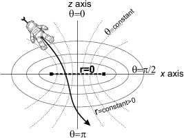
Figure 2: For regular RBH no extension through $r=0$ is required. An observer crossing the surface ($r=0,t=$constant) from positive $z$ to negative $z$ following a non-geodesic time-like curve can stay in its original spacetime. Along the trajectory of the observer $r$ just decreases until reaching the surface $r=0$, where it increases again. The angular B-L coordinates just jump when crossing the disk. In the plane shown in the figure: $\theta\rightarrow\pi-\theta$. (This is somehow similar to following a trajectory crossing $r=0$ in a regular spherically symmetric spacetime equipped with spherical coordinates).

4 The ring

The ring itself requires a separate analysis since neither the Kerr-Schild coordinates nor the Boyer-Lindquist coordinates are well-behaved in the ring (as it is immediate from (2.1),(2.2),(2.3) and (2.5)). A set of coordinates that will help us to analyze the directional behaviour of physical magnitudes around the ring are the toroidal coordinates $\{\rho,\varphi,\psi\}$ (see figure 3), which are related to the Kerr-Schild coordinates through

$$x = (a+\rho\cos\psi)\cos\varphi,$$

$$y = (a+\rho\cos\psi)\sin\varphi,$$

$$z = \rho\sin\psi.$$

Note that in this coordinates the ring is defined by $\rho=0$. The Jacobian determinant of this transformation ($J=-\rho(a+\rho\cos\psi)$) implies that in these coordinates there will be removable coordinate singularities both at the ring and at the $z$ axis.

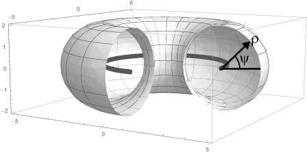
Figure 3: A plot of the behaviour of the toroidal coordinates with the (regular) ring ($\rho=0$) highlighted in black.

From the relationship between K-S and B-L coordinates, it follows that the coordinates $\{\rho,\psi\}$ are related to the Boyer-Lindquist coordinates $\{r,\theta\}$ through

$$r\cos\theta = \rho\sin\psi,$$ (4.1)

$$(r^{2}+a^{2})\sin^{2}\theta = (a+\rho\cos\psi)^{2}.$$

If we do not perform and extension beyond $r=0$ with negative $r$, this implies that around the ring

$$r \simeq \sqrt{a(1+\cos\psi)\rho},$$ (4.2)

$$\cos\theta \simeq \frac{\rho^{1/2}\sin\psi}{\sqrt{a(1+\cos\psi)}}.$$

Note that the metric (2.1) can be interpreted as consisting of a Minkowskian part plus a perturbation. With regard to the perturbation, the behaviour of $H$ around the ring in toroidal coordinates is, from (4.2),

$$H=\frac{\mathcal{M}(r)r^{3}}{r^{4}+a^{2}z^{2}}\simeq\frac{\mathcal{M}(\rho,\psi)}{2}\sqrt{\frac{1+\cos\psi}{a\rho}}.$$

In this way, for a regular RBH with $\mathcal{M}(r)\sim r^{n}$ ($n\geq 3$) one has $H\propto\rho^{(n-1)/2}$ which tends to zero as the ring is approached.

On the other hand, around the ring (2.3) can be written in toroidal coordinates as

$$k_{\alpha}dx^{\alpha}\simeq-dt+ad\varphi-\sqrt{(1+\cos\psi)\frac{\rho}{a}}d\rho+\frac{\rho^{3/2}}{\sqrt{a(1+\cos\psi)}}\sin\psi d\psi.$$

As a consequence, the leading order behaviour of the metric around the ring is just the leading order of the Minkowskian spacetime in toroidal coordinates:

$$ds^{2}\simeq-dt^{2}+d\rho^{2}+\rho^{2}d\psi^{2}+a^{2}d\varphi^{2}.$$

As expected, by not requiring the extension at the disk, the metric around the ring only has a removable coordinate singularity at $\rho=0$ .

As stated in section 2, the effective density ($\mu$) and pressures ($p_{x},\ p_{y}\ \mbox{and}\ p_{z}$) measured by observers with 4-velocity $\mathbf{t}$ can be directly obtained from $\lambda_{1}$ and $\lambda_{2}$. Let us now analyze their dependence on $\rho$ around the ring for a mass function $\mathcal{M}(r)\sim r^{n},\ (n\geq 3)$. With the help of (4.2):

$$\mu=-p_{z} = \lambda_{2}=\frac{2r^{2}\mathcal{M}^{\prime}}{\Sigma^{2}}\sim\rho^{\frac{n-3}{2}}$$

$$p_{x}=p_{y} = -\lambda_{1}=-\frac{2a^{2}\cos^{2}{\theta}\mathcal{M}^{\prime}+r\Sigma\mathcal{M}^{\prime\prime}}{\Sigma^{2}}\sim\rho^{\frac{n-3}{2}}.$$

In this way, the effective density and pressures vanish at the ring for $n>3$. On the other hand, for $n=3$ the densities and pressures are finite functions of the direction of approach to the ring $\psi$. Only in this case the density and pressures are not continuous at the ring. Specifically, for $\mathcal{M}(r)\equiv m_{3}r^{3}+O(r^{4})$ with $m_{3}>0$ a constant,

$$\mu=-p_{z} = \lambda_{2}=6m_{3}\cos^{4}(\psi/2),$$

$$p_{x}=p_{y} = -\lambda_{1}=3m_{3}\cos^{2}(\psi/2)(\cos\psi-3).$$

Note that the effective density is non-negative while the effective pressures are all negative around the ring. These negative effective pressures imply that the weak energy conditions (WEC) are violated near the ring. Nevertheless, this is not surprising since all regular RBH violate the WEC, as shown in [25]. For both the effective density and pressures, the value zero is reached in the direction of the disk $\psi=\pi/2$ and the maximum absolute value is reached in the opposite direction $\psi=0$. Polar plots of the effective density and pressures for this particular case are shown in figure 4.

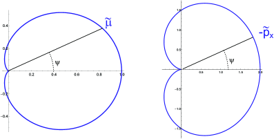
Figure 4: Polar plot of $\tilde{\mu}\equiv\mu/(6m_{3})$ and (minus) $\tilde{p}_{x}\equiv p_{x}/(3m_{3})$ around the ring for the case $\mathcal{M}(r)\sim r^{3}$.

5 Causality

In general, it seems reasonable to ask a time orientable spacetime to be absent of closed causal curves since the existence of such curves would seem to lead to logical paradoxes. A spacetime devoid of closed causal curves is said to be causal [16]. If, in addition, no closed causal curve appears even under any small perturbation of the metric the spacetime is called stably causal. It is well-known that the Kerr metric with the usual extension allowing regions with negative $r$ is non-causal. Since Kerr metric is a particular case of the metric (2.5), it is natural to ask whether regular RBH should also be non-causal.

Along the lines in [18], in order to examine this issue we will use proposition 6.4.9 in [16] that states that when a time function $f$ exists in the spacetime such that its normal $\mathbf{n}\equiv\nabla_{\mu}f\,dx^{\mu}$ is timelike, then the spacetime is stably causal. ($f$ can be thought as the time in the sense that it increases along every future-directed causal curve). Let us choose the time coordinate $\tilde{t}$ in Kerr-Schild coordinates as our time function $f$. The timelike character of $\mathbf{n}$ can be checked as follows:

$$\mathbf{n}^{2}=g^{\mu\nu}\nabla_{\mu}\tilde{t}\nabla_{\nu}\tilde{t}=g^{\tilde{t}\tilde{t}}=-1-\frac{2\mathcal{M}(r)r^{3}}{r^{4}+a^{2}z^{2}}.$$ (5.1)

Since we would like this to be negative, it trivially follows

Proposition 1

[18] If $r\mathcal{M}(r)\geq 0$ for all $r$, then the model of RBH with metric (2.1) [or (2.5)] will be stably causal.

Note that for a regular RBH (unextended through $r=0$), it just suffices to guarantee a non-negative mass function for the spacetime to be stably causal.

6 Global structure

Since regular RBH do not need an extension with regions where $r$ takes negative values, the global structure of these spacetimes will necessarily differ from the global structure of the maximally extended Kerr spacetimes.

In order to get the global structure of regular RBH we would need to locate their null horizons. In the general RBH case we should solve

$$\Delta=r^{2}-2\mathcal{M}(r)r+a^{2}=0.$$ (6.1)

Without the knowledge of a specific $\mathcal{M}(r)$ it is not possible to know the exact position of the horizons. Nevertheless, one can analyze the general behaviour of the horizons by taking into account the following considerations:

• If we assume an asymptotically flat spacetime, at large distances $\mathcal{M}(r)\simeq m=$constant, so that one (approximately) recovers the behaviour for the Kerr solution. Then $\Delta>0$ and $r$ will be a spacelike coordinate.

• For $r\simeq 0$ ($a\neq 0$) a regular RBH has $\Delta>0$ thanks to the effect of the rotation and, again, $r$ will be a spacelike coordinate. (Note that this already happens in the classical Kerr solution).

• If we assume the existence of a RBH and, thus, the existence of an exterior horizon $r_{+}$ (solution of $\Delta=0$) then the continuity of $\Delta$ and the two previous items imply either a single horizon (extreme RBH), two horizons $r_{-}$ and $r_{+}\ (>r_{-})$ or, in general, an even number of horizons.

• If no solutions of (6.1) exist, then no null horizons exist and we are in a hyperextreme case. The regular rotating astrophysical object without an event horizon is not properly a black hole. The regularity implies that, contrary to the classical case, there is not a naked singularity.

In practice, the usual regular RBH in the literature has one or two null horizons, as in the classical case. This is not surprising if one considers deviations from General Relativity as coming from Quantum Gravity effects. Then, based on a simple dimensional analysis, one could expect the Planck scale to be the most natural scale in which to expect the departure from General Relativity to occur, what would imply only strong deviations from the classical solution around $r\sim r_{Planck}$ and, thus, only small corrections to the horizons (at least for RBH with masses much larger than the planckian mass). One also expects that associated with non-singular RBH there would be a weakening of gravity. An effect which should be very important at high curvature scales. In this way, comparing with the classical case, it is usual to obtain bigger inner horizons and smaller outer horizons. Of course, the Planck scale approach could turn out to be too naive and bigger deviations from the classical solutions could be possible, what would be good news for the observational aspects of RBH.

Nevertheless, in order to illustrate the global causal structure of regular RBH let us follow the approach of small perturbations with respect to the classical horizons. In this way, we can have three possible qualitatively different causal structures for the BH spacetime which are represented in the Penrose diagrams of figure 5 (for the case with two null horizons) and of figure 6 (for the extreme case and the hyperextreme case).

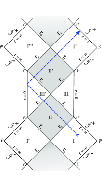
Figure 5: Penrose diagram for a regular rotating black hole with two null horizons. An extension through $r=0$ is not required and, thus, $r\geq 0$ in the maximally extended spacetime. The grey regions are the regions where the coordinate $r$ is timelike. We have depicted a light-like geodesic (dashed blue line) that, starting from the asymptotically flat region I, enters region II by traversing the event horizon $r_{+}$. Then it reaches region III’ by traversing the null horizon $r_{-}$. The value of $r$ first decreases along the geodesic until reaching $r=0$, where it increases again. It makes it to another null horizon $r_{-}$, enters region II’, traverses another event horizon $r_{+}$ to enter the asymptotically flat region I” where it travels towards the future null infinity. (Note that, since there are not singularities, the diagram is valid for all $\theta$).

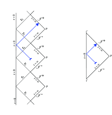
Figure 6: Penrose diagrams for an extreme regular rotating black hole (to the left) and for a hyperextreme case (to the right). In both cases, an extension through $r=0$ is not required and $r\geq 0$. In the extreme case there is only one horizon denoted by $r_{\pm}$ in which the coordinate $r$ is lightlike. $r$ is never timelike. $r_{\pm}$ acts as an event horizon. In the hyperextreme case there are no horizons and $r$ is always spacelike. In both diagrams a light-like geodesic (dashed blue line) travels towards $r=0$, traverses the disk (or ring) and continues its travel towards the future null infinity. (Note that, again, since there are not singularities, the diagrams are valid for all $\theta$).

The absence of an event horizon in the hyperextreme case is interesting, since this implies that an observer could receive information from the inner high curvature regions near $r=0$. In principle, this could be used to observationally test the different approaches to Quantum Gravity. The problem is whether such RBHs are feasible. In the framework of General Relativity, it does not seem possible to obtain such high speed RBH ($a^{2}>m^{2}$) from a collapsing star and any attempt to overspin an existing black hole destroying its event horizon has failed, in agreement with the weak cosmic censorship conjecture. However, for regular RBHs it has been suggested that it could be possible to destroy the event horizon [17].

7 Conclusions

Under suitable conditions, the collapse of an astrophysically significant body can generate a black hole. Since one expects the generator of the black hole to be a rotating body, the black hole will rotate. General Relativity provide us with solutions for rotating black holes and predicts their characteristics, which are compatible with current observations. Nevertheless, the existence of inner singularities in the classical solutions for RBHs and the fact that General Relativity is incompatible with Quantum Mechanics leads us to seek for better singularity-free models for RBHs, often based in some approach to a Quantum Gravity Theory.

Assuming that a manifold endowed with its corresponding metric is a fairly good approximation for describing regular RBHs, most of the models in the literature are of the Gürses-Gürsey type. Remarkably, the analysis of these regular RBHs lead us to conclude that regular RBHs do not require an extension through their disk. As a consequence, causality problems could be avoided simply if their mass function is non-negative (what seems a desirable property of the mass function).

With regard to the (regular) ring, it has been shown that it is devoid of conical singularities. The effective density and pressures vanish at the ring if $\mathcal{M}(r)\sim r^{n}$ with $n>3$. By contrast, in the particular case $\mathcal{M}(r)\sim r^{3}$ one expects observers to measure a jump in the (finite) effective density and pressures (with a specific directional character) while crossing the ring. Note that this is somehow similar to the situation that an observer detects when crossing a star’s surface modelled by matching, for instance, an exterior vacuum field with an interior fluid [22]. It implies that in the $n=3$ case there exists a local coordinate system in which the metric will be just $C^{1}$ at the ring.

In summary, contrary to classical RBH solutions, regular RBH avoid singularities, the violation of the cosmic censorship conjecture, the existence of regions where the mass function acts repulsively and causality violations.

References

- [1] Azreg-Aïnou M 2014 Phys. Rev. D 90 064041 (arXiv:1405.2569 [gr-qc])
- [2] Bambi C and Modesto L 2013 Phys. Lett. B 721 329 (arXiv:1302.6075 [gr-qc])
- [3] Bambi C, Modesto L and Rachwal L 2017 JCAP 05 003 (arXiv:1611.00865 [gr-qc])
- [4] Bardeen J M 1968 Conference Proceedings of GR5 p.174
- [5] Burinskii A 2002 Czech.J.Phys. 52 C471
- [6] Caravelli F and Modesto L 2010 Class.Quant.Grav. 27 245022 (arXiv:1006.0232 [gr-qc])
- [7] Carter B 1968 Phys. Rev. 174 1559
- [8] De Lorenzo T, Giusti A and Speziale S 2016 Gen. Rel. and Grav. 48 31. Corrigendum at Gen. Rel. and Grav. 48 111
- [9] Dymnikova I and Galaktionov E 2015 Class. Quant. Grav. 32 165015 (arXiv:1510.01353 [gr-qc])
- [10] Fayos F, Martín-Prats M M and Senovilla J M M 1995 Class. Quantum Grav. 12 2565
- [11] Franzin E, Liberati S, Mazza J and Vellucci V 2022 arXiv:2207.08864 [gr-qc]
- [12] Ghosh S G 2015 Eur. Phys. J. C 75 532 (arXiv:1408.5668 [gr-qc])
- [13] Gomes H and Herczeg G 2014 Class.Quant.Grav. 31 175014 (arXiv:1310.6095 [gr-qc])
- [14] Griffths J B and Podolský J 2009 Exact space-times in Einstein’s General Relativity Cambridge: Cambridge University Press.
- [15] Gürses M and Gürsey F 1975 Phys. Rev. D 11 967
- [16] Hawking SW and Ellis GFR 1973 The large scale structure of space-time Cambridge University Press, Cambridge
- [17] Li Z and Bambi C. 2013 Phys.Rev.D 87 124022 (arXiv:1304.6592 [gr-qc])
- [18] Maeda H 2021 (arXiv:2107.04791 [gr-qc])
- [19] Mazza J, Franzin E and Liberati S 2021 JCAP 04 082
- [20] Misner CW, Thorne KS and Wheeler JA 1970 Gravitation, W.H. Freeman and Company, New York
- [21] Reuter M and Tuiran E 2011 Phys. Rev. D 83 044041
- [22] Senovilla JMM 1998 Gen. Rel. Grav. 30 701
- [23] Simpson A and Visser M 2022 JCAP 03 011 (arXiv:2111.12329 [gr-qc])
- [24] Smailagic A and Spallucci E 2010 Phys. Lett. B 688 82 (arxiv:1003.3918 [hep-th])
- [25] Torres R and Fayos F 2017 Gen. Rel. and Grav. 49 2 (arXiv:1611.03654 [gr-qc])
- [26] Torres R 2017 Gen. Rel. and Grav. 49 74 (arXiv:1702.03567 [gr-qc])
- [27] Toshmatov B, Ahmedov B, Abdujabbarov A and Stuchlik Z 2014 Phys. Rev. D 89 104017 (arXiv:1404.6443 [gr-qc])