Binary vision: The merging black hole binary mass distribution via iterative density estimation

Abstract

Binary black hole (BBH) systems detected via gravitational-wave (GW) emission are a recently opened astrophysical frontier with many unknowns and uncertainties. Accurate reconstruction of the binary distribution with as few assumptions as possible is desirable for inference on formation channels and environments. Most population analyses have, though, assumed a power law in binary mass ratio $q$, and/or assumed a universal $q$ distribution regardless of primary mass. Kernel density estimation (KDE)-based methods allow us to dispense with such assumptions and directly estimate the joint binary mass distribution. We deploy a self-consistent iterative method to estimate this full BBH mass distribution, finding local maxima in primary mass consistent with previous investigations and a secondary mass distribution with a partly independent structure, inconsistent with both power laws and with a constant function of $q$. We find a weaker preference for near-equal mass binaries than in most previous investigations; instead, the secondary mass has its own “spectral lines” at slightly lower values than the primary, and we observe an anti-correlation between primary and secondary masses around the $\sim\!10\,M_{\odot}$ peak.

O0pt O0pt$\mathrlap{\mathchoice{\raisebox{0.0pt}{$\displaystyle{\mathchar 22\relax\mkern-9.0mu}$}}{\raisebox{0.0pt}{$\textstyle{\mathchar 22\relax\mkern-9.0mu}$}}{\raisebox{0.0pt}{$\scriptstyle{\mathchar 22\relax\mkern-9.0mu}$}}{\raisebox{0.0pt}{$\scriptscriptstyle{\mathchar 22\relax\mkern-9.0mu}$}}}b$

1 Introduction

Ever since the first GW detection revealed a binary black hole source with the—previously unsuspected—component masses of around 35 $M_{\odot}$ (Abbott et al., 2016a, b), LIGO-Virgo-KAGRA observations of compact binaries have continued to yield surprises, of which the binary mass distribution arguably contains the most information bearing on formation environments and channels. In the first three observing runs of Advanced LIGO (Aasi et al., 2015) and Advanced Virgo (Acernese et al., 2015) the better part of 100 detections of binary compact object mergers via gravitational wave (GW) emission were made, as catalogued in the GWTC releases (Abbott et al., 2019, 2021, 2021a, 2021b). Having a set of detected events it is possible to study population properties of these compact binaries and eventually draw implications from these properties on binary astrophysical formation and evolution. Detailed investigations of the population properties of BBH mergers, the most commonly detected source type, were undertaken in Abbott et al. (2020a, 2023a), focusing on several population characteristics including their component masses and spins and possible dependence on redshift.

Among parameters estimated and studied in connection with the population properties of binary compact objects, the component masses are obtained with least uncertainty. Many parameterized and semi- or non-parametric models have been proposed to study the mass-dependence of the compact binary merger rate or the mass distribution of the merger population (see Abbott et al., 2023a, and references therein). In parametric models, Bayesian hierarchical techniques are used to infer model hyper-parameter posteriors, and thus the population distribution (e.g. Mandel, 2010; Thrane & Talbot, 2019). On the other hand, non-parametric models are data driven methods which learn population properties either without requiring any specific functional form, or (for semi-parametric models) allowing for generalised deviations from a given parametric model (Powell et al., 2019; Tiwari & Fairhurst, 2021; Tiwari, 2021, 2022; Veske et al., 2021; Rinaldi & Del Pozzo, 2021; Edelman et al., 2021, 2023; Callister & Farr, 2023; Ray et al., 2023; Toubiana et al., 2023).

In Sadiq et al. (2022) we introduced a fast and flexible adaptive width kernel density estimation (awKDE) as a non-parametric estimation method for population reconstructions of binary black hole distribution from observed gravitational wave data. A limitation of this method arose from the measurement uncertainty in each individual event’s parameters. Given the relatively low signal-to-noise ratios, the observed component masses have significant uncertainties (e.g. Veitch et al., 2015) that can bias the overall population distribution if not properly accounted for.

In this work we are proposing a new method to reduce this uncertainty estimate in our populations distribution by using iterative re-weighting scheme of samples for each observed events using the awKDE density estimates as a probability for re-weighting of samples. The idea is similar to the standard expectation-maximization algorithm (Dempster et al., 1977).

As an application of this new method, we estimate the full 2-dimensional component mass distribution without assumptions (aside from the use of Gaussian kernels) on its functional form. While attention has often focused on the primary component mass or on the more precisely measured chirp mass (see among others Dominik et al., 2015; Tiwari & Fairhurst, 2021; Tiwari, 2022, 2023; Edelman et al., 2023; Schneider et al., 2023; Farah et al., 2023), less attention has been paid to the full binary distribution, either considered via the secondary $m_{2}$ or mass ratio $q\equiv m_{2}/m_{1}$. We expect these parameters to bear traces of the possible BBH formation channels (Kovetz et al., 2017), in that for dynamical (cluster) formation the two masses may be independent variates, up to a factor modelling probability of binary formation and merger (Fishbach & Holz, 2020; Antonini et al., 2023) that typically favors near-equal masses (e.g. Rodriguez et al., 2016; O’Leary et al., 2016); whereas for isolated binary evolution, some nontrivial though probably highly model-dependent correlation of component masses may arise (e.g. van Son et al., 2022).

Typically, parametric models have assumed power-law $m_{2}$ dependence at fixed $m_{1}$ (Kovetz et al., 2017; Fishbach & Holz, 2017; Talbot & Thrane, 2018; Abbott et al., 2019), recovering mildly positive powers indicating a preference for equal masses. A more detailed study using GWTC-1 events concluded that the two BHs of a given binary prefer to be of comparable mass (Fishbach & Holz, 2020). More recent non-parametric or semi-parametric studies have relaxed these assumptions, either through allowing the power-law index to vary over chirp mass (Tiwari, 2022), or allowing $p(q)$ to be a free (data-driven) function (Edelman et al., 2023; Callister & Farr, 2023) though enforcing the same dependence over all primary masses. Tiwari (2023) introduced a more flexible approach with $p(q)$ modelled by a truncated Gaussian whose parameters depend on chirp mass, finding some significant variation. Ray et al. (2023) measured the full 2-d distribution with a binned (piecewise-constant) model over $m_{1}$, $m_{2}$ (including possible redshift dependence), although they did not consider the $q$ distribution. Note that the mass ratio distribution presents nontrivial technical issues since (at least for lower mass BBH) typical event measurement errors are both large, and correlated with the BH orbit-aligned spin components (Cutler & Flanagan, 1994; Baird et al., 2013). Concerning measurement errors, we expect our iterative reweighting scheme to yield a significant advance in reconstructing the full mass distribution.

The remainder of the paper is organized as follows: in section 2 we explain our method and demonstrate it using simple one-dimensional mock data. In section 3 we apply our method to detected BBH in GWTC-3, compare the result with our previous studies and further use our new method in two mass dimensions. In section 4 we discuss the implications of our results and consider extensions of the method. We also describe additional mock data tests and supplementary results in appendices.

2 Method

2.1 Statistical framework

Our general approach to population inference can be considered as similar to maximum likelihood, with uncertainties quantified via empirical bootstrap methods (Efron, 1979). Given a set of observed events, if we neglect measurement uncertainty in each event’s parameters, our population estimate is a KDE where the kernel bandwidth for each event is adjusted (Breiman et al., 1977; Abramson, 1982; Terrell & Scott, 1992; Sain & Scott, 1996) using an adaptive scheme to maximize the cross-validated likelihood (Sadiq et al., 2022). Note that a “maximum likelihood” KDE is not well defined, as the likelihood increases indefinitely in the limit of small bandwidth kernels centered on the observations; in this limit, the variance of the density estimate over realizations of the data becomes infinitely large. The bias-variance tradeoff is then addressed by adaptive kernel bandwidth, with a choice of hyperparameters—global bandwidth $h$ and sensitivity parameter $\alpha$, see Wang & Wang (2011)—optimized by grid search using leave-out-one cross-validation to calculate a figure of merit. We then quantify counting uncertainties for the underlying inhomogeneous Poisson process using generalized bootstrap resampling Chamandy et al. (2012).

We noted in Sadiq et al. (2022) that for nontrivial measurement errors this method, in addition to possible intrinsic biases due to the choice of a Gaussian KDE, will be biased towards an over-dispersed estimate of the true distribution. Here we motivate and present our strategy for correcting this bias. Our motivation is linked to Bayesian hierarchical population inference (Mandel, 2010), where measurement errors are treated by considering the true event properties $\vec{\theta_{i}}$ for events labelled $i=1,\ldots,N$ as nuisance parameters in the likelihood:

$$p(\{d\}|\vec{\lambda})=\prod_{i=1}^{N}\int p(d_{i}|\vec{\theta}_{i})p(\vec{\theta}_{i}|\vec{\lambda})\,d\vec{\theta}_{i},$$ (1)

where $\{d\}$ is the set of data segments $d_{i}$ corresponding to the events and $\vec{\lambda}$ are population model hyperparameters (here for simplicity we omit selection effects). Inference is implemented using parameter estimation (PE) samples which were generated using a standard or fiducial prior $p_{\rm PE}(\vec{\theta})$, often chosen as uniform over parameters of interest (see e.g. Veitch et al., 2015; Thrane & Talbot, 2019). Samples (labelled by $k$) are distributed as the posterior density using this prior, hence

$$\vec{\theta}_{i}^{k}\sim p(\vec{\theta}_{i}|d_{i},p_{\rm PE}(\vec{\theta}))\propto p(d_{i}|\vec{\theta}_{i})p(\vec{\theta}_{i}|\vec{\lambda})\cdot\frac{p_{\rm PE}(\vec{\theta})}{p(\vec{\theta}_{i}|\vec{\lambda})},$$ (2)

hence the integrals may be performed (up to a constant factor) by summing over samples re-weighted by the ratio of the population distribution to the PE prior, $p(\vec{\theta}_{i}|\vec{\lambda})/p_{\rm PE}(\vec{\theta})$.

Here, while not making use of this hierarchical likelihood, we remark that PE samples give a biased estimate of each event’s properties if the true population distribution $p_{\rm pop}(\vec{\theta})$ (corresponding to $p(\vec{\theta}|\vec{\lambda})$ in the parameterised case) is not equal to $p_{\rm PE}(\vec{\theta})$. Then, if we have access to an estimated population distribution $\hat{p}_{\rm pop}(\vec{\theta})$ that is more accurate than the PE prior is, we will obtain more accurate estimates of event properties by drawing samples weighted proportional to $\hat{p}_{\rm pop}(\vec{\theta})/p_{\rm PE}(\vec{\theta})$, as described in more detail below,

To summarize, a KDE obtained by drawing from PE samples will be biased because these samples are themselves biased, due to the PE prior not being equal to the true population distribution. However, the more accurate an estimate of the true distribution we are able to obtain, the smaller will be the bias in event parameters using reweighted PE samples, and ultimately the smaller will be the bias of the KDE.

2.2 Iterative Reweighting

The above discussion suggests an iterative procedure where, beginning with both biased PE samples and a biased population KDE, one may be improved in turn using the other, until – ideally – reaching a stationary state, where both the sample draws and the corresponding population estimates are unbiased (up to more fundamental limitations of PE and of our KDE). This iterative strategy is similar to the Expectation-Maximization (EM) algorithm (Dempster et al., 1977), a popular method to estimate parameters for statistical models when there are missing or incomplete data.

Our basic algorithm follows these steps:

1. For each GW event, draw Poisson distributed (with mean 1) PE samples weighted by the current estimate of population density $\hat{p}_{\rm pop}$

2. Create an awKDE from this sample set, optimizing the global bandwidth (and sensitivity parameter $\alpha$, if not fixed)

3. Update the current population estimate using one or more KDEs and the selection function, and go to step 1.

In more detail, in step 1 we draw PE samples with probability proportional to the ratio of $\hat{p}_{\rm pop}(\vec{\theta}_{i}^{k})$ to the PE prior distribution. Step 2 reproduces our previous awKDE method. Step 3 relates the KDE of detected events to an estimate of the true population distribution, hence in general it requires us to compensate for the selection function over the event parameter space: i.e. we estimate the true distribution by the KDE of detected events divided by the probability of detection, as detailed in (Sadiq et al., 2022, section 3.1).

In step 3 we may choose to derive the updated population density $\hat{p}_{\rm pop}(\vec{\theta})$ from only the most recently calculated KDE: then the iterative process is a Markov chain, and we may characterize it via the autocorrelation of various scalar quantities computed at each iteration. We use the optimized global bandwidth $h$ (and adaptive sensitivity parameter $\alpha$, if not fixed to unity) for this purpose.

After discarding a small number of initial iterations and then accumulating a number significantly greater than the autocorrelation time, we expect the collection of iterations to provide unbiased (though not necessarily independent) estimates of the population distribution. For subsequent iterations we then use the median of $\hat{p}_{\rm pop}(\vec{\theta}_{i}^{k})$ over a buffer of previous iterations (usually the previous 100) to determine the sample draw probabilities for the next iteration. This population estimate should be more precise than one using only a single previous KDE; and in addition using the buffer estimate the samples for each successive iteration are essentially independent.

2.3 One-dimensional mock data demonstration

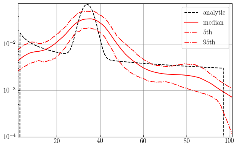
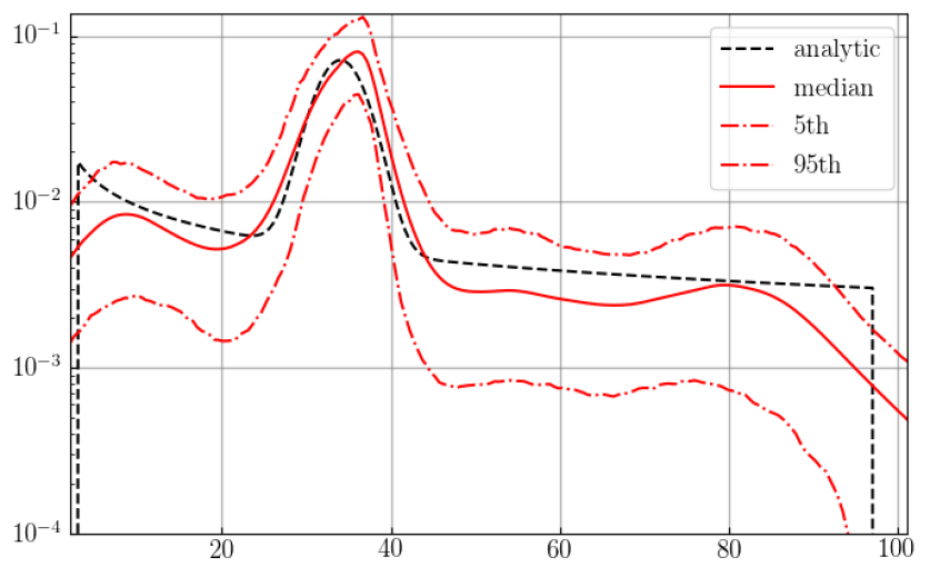
Figure 1: awKDE for 60 events from a mock data mixture distribution with 50% power law ($\alpha=-0.5$) and 50% Gaussian ($\mu=35$, $\sigma=3$) samples. 100 mock parameter samples are generated for each event with measurement error $\sigma_{m}=5$. Top: awKDE drawing random parameter samples without reweighting. Bottom: applying iterative reweighting. The solid (dot-dashed) lines represent the median (symmetric 90% confidence band) from 900 bootstrap iterations.

We first test this iterative reweighting method on a simple mock dataset. We generate true event parameters drawing 30 event each from a truncated power law and a Gaussian distribution respectively; the power law is $p(x)\sim x^{-0.5}$ and the Gaussian has mean (s.d.) of $\mu=35$ ($\sigma_{p}=3$). We then add measurement errors to our true parameters with a s.d. $\sigma_{m}=5$, hence broader than the true Gaussian peak; 100 mock parameter samples with the same uncertainty are then generated around each “measured” value. First, applying awKDE as in Sadiq et al. (2022) to random draws from these mock parameter samples, as expected we find an over-dispersed estimate around the peak (Fig. 1, top).

The second (bottom) plot of Fig. 1 shows the awKDE applying our iterative reweighting algorithm. Here the Gaussian height and s.d. are accurately reconstructed and the true distribution is well within the 90% percentiles of iteration samples, except at the step-function truncation of the power law which cannot be accurately represented by a Gaussian KDE.

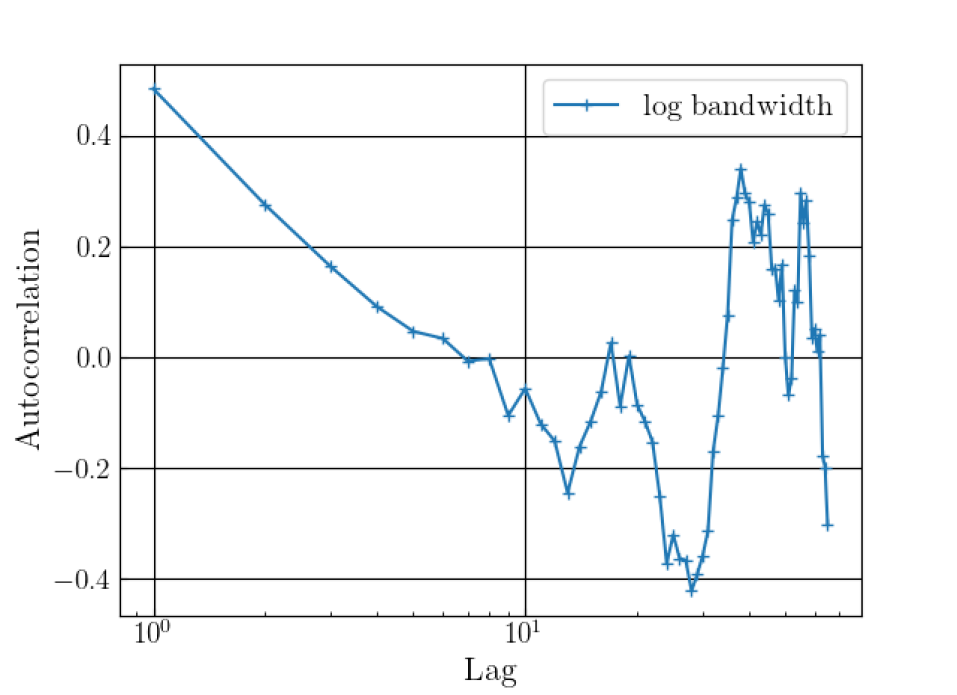
Figure 2: Autocorrelation of the (log) optimized global bandwidth series for the iterative Markov chain. The x-axis shows lag, i.e. separation of the iterations between which autocorrelation is calculated.

We verify that the initial Markov process has accumulated several independent samples by plotting the autocorrelation of the optimized global bandwidth $h$ vs. lag (separation along the chain) in Fig. 2. (We fix the adaptive sensitivity parameter $\alpha$ to unity for 1-d data.) The autocorrelation drops near zero by a lag of $\lesssim\!10$ iterations, thus a buffer of 100 iterations contains several independent population estimates. The estimate is more noisy for larger lags as fewer iterations are available.

More detailed tests of iterative reweighting with a Gaussian KDE in two dimensions in the presence of correlated parameter errors are given in Appendix A.

3 Results from GWTC-3

As in Sadiq et al. (2022), as input to our analysis we use parameter estimation samples (LVK, 2021a) for the set of BBH events catalogued in GWTC-3 (Abbott et al., 2021a, 2023b) with false alarm rate below 1 per year. For the sensitivity estimate we employ a fit to search injection (simulated signal) results (Wysocki et al., 2019; Wysocki, 2020) released with the catalog (LVK, 2021b).

3.1 One-dimensional mass distribution

We start by evaluating the effect of the iterative reweighting method on the 1-d primary mass distribution, taking 100 random PE samples for each of the 69 BBH events; here, we assume a power-law distribution for secondary mass $p(m_{2})\sim q^{1.5}$. We reproduce the awKDE results from Sadiq et al. (2022) and use this estimate to seed the reweighted iteration algorithm. After $\sim$1000 reweighting iterations we compute the median and symmetric 90% interval from the last 900 rate estimates (the first 100 are used to set up a buffer for population weighting, as above): results are presented in Fig. 3.

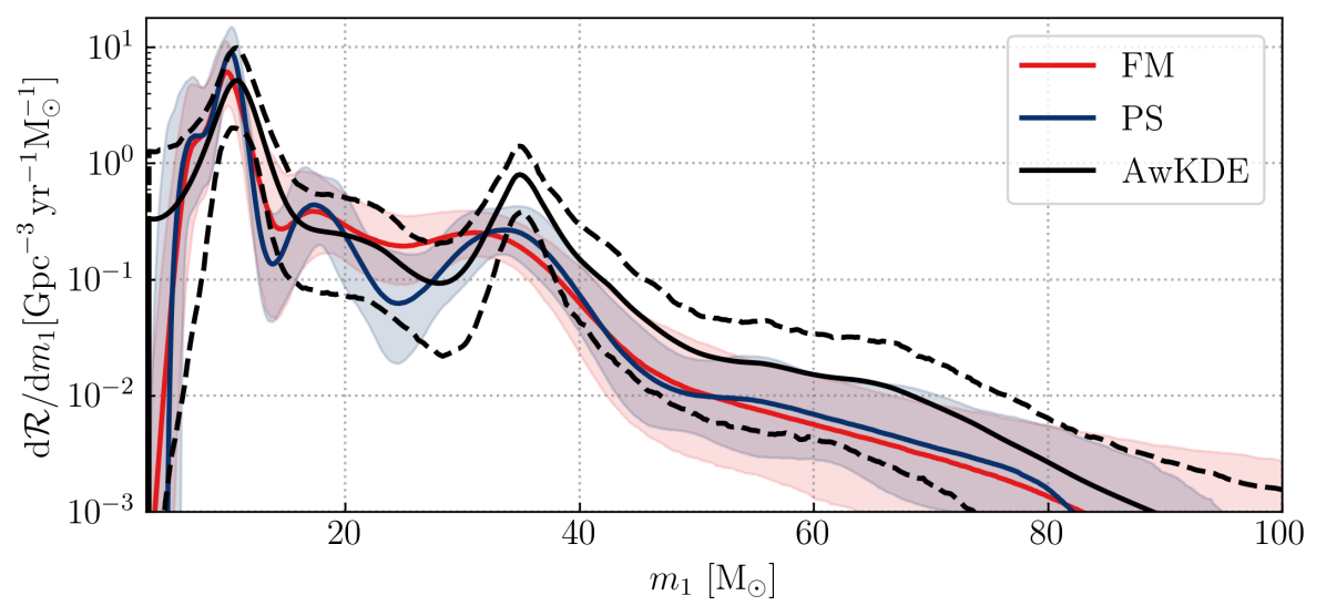
Figure 3: Differential rate over BBH primary mass using the iterative weighted KDE on GWTC-3 PE samples, assuming a power-law secondary distribution. We overplot our estimates with two of the models, Flexible mixtures (FM), and Power Law + Spline (PS) models in (Abbott et al., 2023a). Our estimate is generally consistent with other non-parametric methods, though with a higher and narrower peak around $35\,M_{\odot}$ and lacking any feature between the 10 $M_{\odot}$ and 35 $M_{\odot}$ peaks.

Our estimate is generally consistent with other non-parametric or semi-parametric approaches, represented by the Flexible mixtures, and Power Law + Spline models in Abbott et al. (2023a), and does not show the over-dispersion apparent in Figure 8 of Sadiq et al. (2022); specifically, we find a slightly higher and narrower peak around $35\,M_{\odot}$, but no identifiable feature around $20\,M_{\odot}$ (compare Tiwari, 2022; Toubiana et al., 2023).

3.2 Two—dimensional Mass Reconstruction

Next, we apply our reweighting scheme on PE samples for both component masses and compute the two-dimensional (2-d) merger rate, using the estimated sensitive volume$\times$time (VT) as a function of the two masses. We will first discuss various technical aspects of extending the 1-d calculation without assuming any power-law dependence for $m_{2}$.

Binary exchange symmetry

Typically when presenting binary parameter estimates, the convention $m_{1}>m_{2}$ is applied. However, all aspects of binary formation physics and event detection and parameter estimation will be invariant under swapping the component labels, i.e. exchanging $m_{1}\leftrightarrow m_{2}$ (and at the same time exchanging the spins). Thus, considering the differential merger rate $\mathcal{R}(m_{1},m_{2})$ as a function over the whole plane, it must also have a reflection symmetry about the line $m_{1}=m_{2}$. To respect this symmetry and remove biases resulting from the apparent lack of support at $m_{2}>m_{1}$, we train and evaluate KDEs on reflected sample sets which contain both the released PE samples, and copies of them with swapped components. Note also that a power-law $m_{2}$ distribution implies the rate is a non-differentiable function at the equal mass line, whereas a KDE by construction is smooth and differentiable everywhere.

Choice of KDE parameters

In previous work (Sadiq et al., 2022), we mainly considered a KDE constructed over linear mass (or distance) parameters; however, here we choose the logarithms of component masses. While this choice is not expected to have a large impact on the results, since the kernel bandwidth is free to locally adapt in either case, it is technically preferable for a few reasons: we avoid any possible KDE support at negative masses; there is a generally higher density of events towards lower masses considering the entire $3-100\,M_{\odot}$ range; the density of observed events also shows less overall variation over log coordinates; and when evaluating the KDE on a grid with equal spacing, fewer points are required to maintain precision for the low-mass region.

For a 2-d KDE we also have a choice of kernel parameters, i.e. the Gaussian covariance matrix: given the similar or identical physical interpretation and range of values between $\ln m_{1}$ and $\ln m_{2}$, we choose a covariance proportional to the unit matrix, with an overall factor determined by the local adaptive bandwidth for each event.

PE prior

The PE samples released by LVK use a prior uniform in component masses (LVK, 2021a) up to a factor dependent on cosmological redshift; we currently do not consider reweighting relative to the default PE cosmological model. As the prior is a density, it transforms with a Jacobian factor when changing variables to $\ln m_{1},\ln m_{2}$, thus, we must divide the estimated rate $\mathcal{R}(\ln m_{1},\ln m_{2})$ by a prior $\propto m_{1}m_{2}$ when obtaining reweighted draw probabilities.

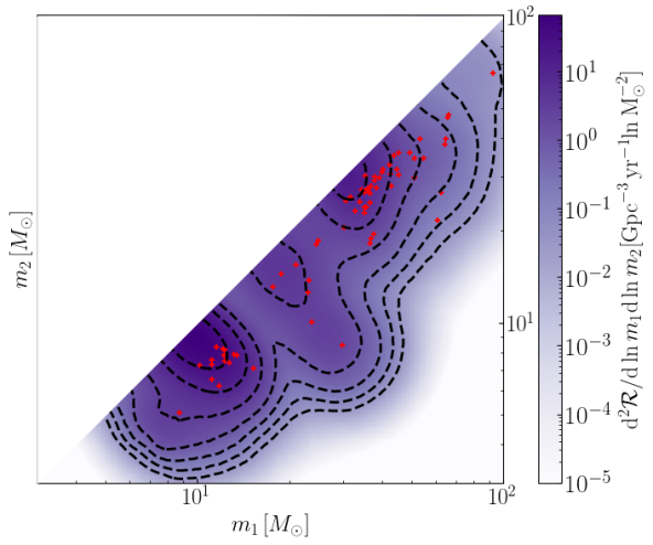
Figure 4: Two dimensional rate estimated from PE samples for 69 BBH events from GWTC-3. Red $+$ symbols show the median masses for each event. The contours and color scale shows the two-dimensional differential merger rate over $\ln m_{1},\ln m_{2}$ from iterative reweighted KDE. Two main maxima are visible at $m_{1}\,(m_{2})\sim 10\,(8)\,M_{\odot}$ and $\sim\!35\,(32)\,M_{\odot}$ with a possible less significant overdensity around $m_{1}\sim 20\,M_{\odot}$.

With these technical choices, we perform 1500 reweighting iterations in total, the first 600 using the Markov chain (i.e. the immediately preceding rate estimate) for sample draw weights, and the remaining 900 using the buffer median estimate.

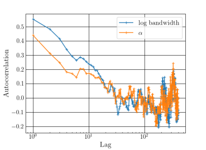
Figure 5: Autocorrelations of the KDE (log) global bandwidth and adaptive parameter $\alpha$ using the initial 600 Markov chain iterations. The autocorrelation drops close to 0 by a lag of $\sim$30 iterations. The estimate becomes noisy at high lags as a smaller number of iterations is available.

Fig. 4 shows the rate estimate computed with iterative reweighting for BBH events in GWTC-3. The autocorrelations of optimal global bandwidth and sensitivity parameter $\alpha$ for the first 600 iterations are shown in Fig. 5: the correlation drops close to $0$ at a lag of $\sim\,$30 iterations.

The mass distribution shows several interesting features in addition to the expected peaks (overdensities) around primary masses of $\sim\!10\,M_{\odot}$ and $\sim\!35\,M_{\odot}$, with corresponding peaks over secondary mass. For primary masses $\sim\!35\,M_{\odot}$ up to $80\,M_{\odot}$, the most likely secondary mass is $\sim\!30\,$–$\,35\,M_{\odot}$. Thus, over this range the two component masses appear almost independently chosen. Around the $m_{1}\sim 10\,M_{\odot}$ peak, there appears to be some anti-correlation of the two components, i.e. higher $m_{1}$ favors lower $m_{2}$. Between the two peaks the distribution of mass ratios appears broader than at either one (as hinted at in Tiwari, 2023), although the apparent trend is based on a small number of events. We also see a narrow lower density region just above the $\sim\!10\,M_{\odot}$ peak (cf. the local minimum at chirp mass $\sim\!11\,M_{\odot}$ in Tiwari 2023).

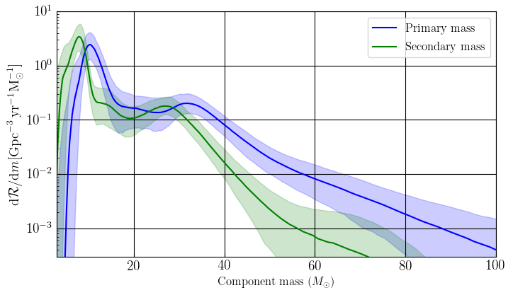
Figure 6: Merger rates over component masses, obtained by numerical integration of our 2-d KDE rate estimates in Fig. 4: the medians and symmetric 90% confidence regions are shown.

We also integrated the 2-d KDE rate estimate numerically over both $m_{1}$ and $m_{2}$ to obtain merger rates over component mass. As shown in Fig. 6, we recover features consistent with the 2-d estimates and with other methods. Each component mass distribution appears well modelled by a combination of two Gaussian peaks and (broken) power laws.

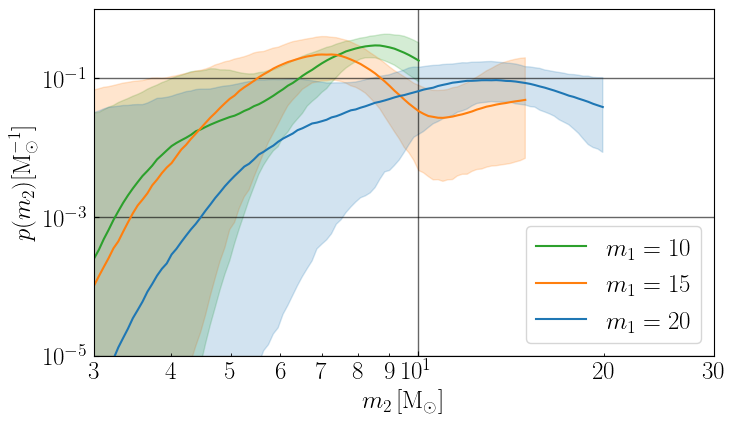
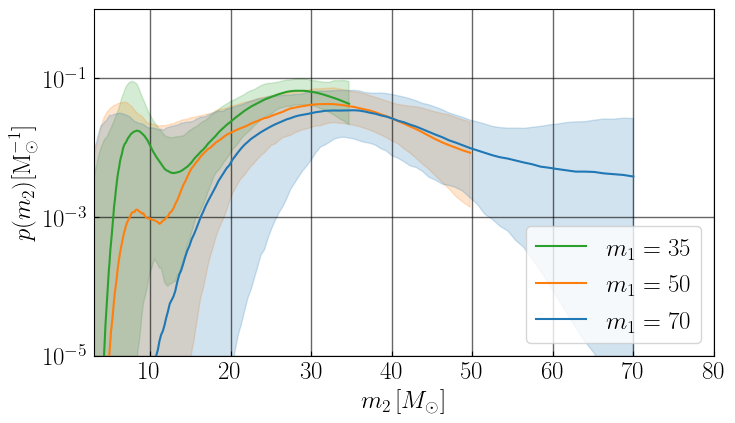
Figure 7: Secondary mass $m_{2}$ distributions estimated via iterative reweighted KDE for various fixed values of primary mass: for each $m_{1}$ (in $M_{\odot}$) we plot the median and symmetric $90\%$ confidence band. Notice the top plot x-xais is in log scale unlike the bottom plot with linear scale in $x$-axis.

To elucidate features in the 2-d distribution, we choose various representative values of primary mass to plot the distribution of $m_{2}$ in Fig. 7. The similarity between secondary distributions for $m_{1}\gtrsim 35\,M_{\odot}$ is evident.

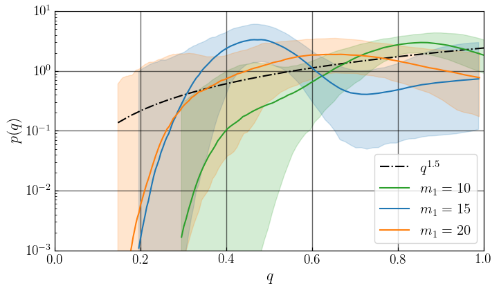
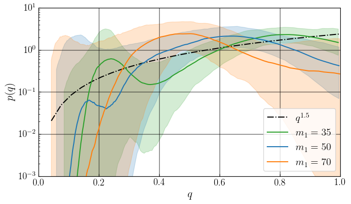
Figure 8: Mass ratio $q$ distributions estimated via iterative reweighted KDE for various fixed values of primary mass: for each $m_{1}$ (in $M_{\odot}$) we plot the median and symmetric $90\%$ confidence band. For comparison we overplot a power law dependence $\propto q^{1.5}$.

We may also derive the distribution of mass ratio $q$ from our 2-d rate estimate. We plot this for various representative values of primary mass in Fig. 8, and compare to a typical power law $\propto q^{1.5}$. First, we see that the $q$ distribution varies over primary mass; hence, models where it is forced to the same form over the whole mass range are likely to have nontrivial bias. For some primary masses, $p(q)$ is consistent with a monotonic increasing function such as a positive power, but for others it clearly decreases over some of the range. Roughly, if $m_{1}$ is close to a peak then $p(q)$ is consistent with an increasing power law, but for other values the mass ratio rather shows a maximum at intermediate values, down to $q\sim 0.5$ for $m_{1}=15$ or $m_{1}=70$.

This behaviour may suggest that the primary and secondary masses are independently drawn from similar distributions, modulo a $q$-dependent “pairing factor” (Fishbach & Holz, 2020) which influences the relative probability of binary merger. However the preference towards $q\sim 1$ seen in previous work is not confirmed here. Callister & Farr (2023) reached a similar conclusion although assuming a “universal” $p(q)$ over all primary masses.

Results including GW190814

We also estimate the 2-d and 1-d integrated merger rates using our iterative reweighted KDE method when the outlier event GW190814 (Abbott et al., 2020b), which has a mass ratio $\mathcal{O}(10)$ and a secondary mass barely above the likely neutron star maximum mass, is included in the BBH population. Detailed results are presented in Appendix B: roughly summarizing the trends seen there, the bulk of the estimated distribution remains little changed by the addition of the extra event, although the peak in secondary mass below $10\,M_{\odot}$ is shifted towards lower values and both higher and broader; this is likely due to a general increase in KDE bandwidth when optimized with cross-validation. (In parameterized models the estimated mass distribution is also highly sensitive to inclusion of GW190814 (Abbott et al., 2020a, 2023a).) It is not clear whether other methods for bandwidth choice would yield more accurate estimates; higher event statistics in the low $m_{2}$ regime are clearly desirable.

4 Discussion

Summary of results

In this work we undertook a detailed investigation of the full 2-d mass distribution of merging compact binary black holes observed by LIGO-Virgo-KAGRA up to the O3 run without assuming any specific functional form for the secondary mass or mass ratio, enabled by a new method of iterative density estimation to address mass measurement uncertainties. Although we reproduce the broad features and local maxima seen in other parametric and non-parametric analyses, we find significantly less preference for near-equal masses than in most previous works; we also find that the mass ratio distribution cannot be described by a single function over the whole population (compare Tiwari, 2023). For a range of primary masses, we find non-monotonically varying secondary and mass ratio distributions, thus a power-law dependence is ruled out. Furthermore, we find that for primary masses above $35\,M_{\odot}$ the secondary mass distribution is nearly independent of $m_{1}$, with a “preferred partner” mass of $m_{2}\simeq 30-35\,M_{\odot}$. Conversely, near the low-mass peak $m_{1}\simeq 10\,M_{\odot}$ we observe an anticorrelation between the two components, i.e. higher $m_{1}$ implies lower $m_{2}$.

Possible astrophysical interpretations

Our new estimate of the joint $m_{1}$–$m_{2}$ distribution may be compared to model predictions in the literature; because our individual component marginal distributions are similar to previous findings, we focus here on the mass ratio. Broadly speaking, we can distinguish model predictions from the isolated binary and dynamical channels.

The isolated binary channel predicts relatively flat $p(q)$ distributions (e.g. Belczynski et al., 2020; Olejak et al., 2021) compared to the dynamical channel (see Fig. 2 in Baibhav et al. 2023 and Fig. 1 in Zevin et al. 2021). Our estimates show in general flatter $q$ distributions than the GWTC-3 results presented in Abbott et al. (2023a).

Because predictions for $p(q)$ in the isolated binary channel depend strongly on the adopted parameters (see e.g. Broekgaarden et al., 2022), our results provide an important step towards constraining astrophysical parameters with GWs. For example, the steep $p(q)$ found for very small common envelope efficiency parameter ($\alpha_{\rm CE}\simeq 0.2$, Baibhav et al., 2023) and the chemically homogeneous evolution model (Mandel & de Mink, 2016) seem disfavoured, implying that these routes cannot account for the majority of the observed population.

The stable mass transfer channel is efficient for primary masses near $\sim\!10\,M_{\odot}$. van Son et al. (2022) predicts a dearth of near-equal mass mergers, which is because the binary needs to be relatively unequal in mass during the second mass transfer phase for the orbit to shrink, but not too unequal to avoid unstable mass transfer. This is only partly supported by our Fig. 4 in that the low-mass peak has support from equal mass out to $q\simeq 0.5$. For some parameter choices their models predict bi-modality in $p(q)$, with peaks at $q\simeq 0.35$ and $q\simeq 0.75$: our results suggest a peak at $q\simeq 0.8$ for $m_{1}\simeq 10\,M_{\odot}$ and at $q\simeq 0.45$ for $m_{1}\simeq 15\,M_{\odot}$ (see Fig. 8), suggesting that a more detailed comparison may yield interesting constraints.

For the dynamical channel, it is interesting to consider whether models now predict $q$ distributions that are too steeply rising. Rodriguez et al. (2016) modelled BBH mergers that formed dynamically in globular clusters: they find a median mass ratio of 0.87, with 68% of sources having mass ratios $q>0.8$. As shown in Fig. 8 we find comparable support for near-equal mass only at $m_{1}\sim 10\,M_{\odot}$ or $\sim\!35\,M_{\odot}$; elsewhere our median $q$ is significantly lower.

Antonini et al. (2023) model BBH merger in globular clusters in comparison to the GWTC-3 $q$ distribution: their model distributions are flatter and underestimate the power-law LVK fits by an order of magnitude at $q\simeq 1$. They find a final $q$ distribution flatter than the $q$ distribution of dynamically formed BBHs ($p(q)\propto q^{4}$ for metal-poor clusters) because the BH mass function is not always sufficiently sampled, such that a secondary BH with a mass similar to the primary is present in a cluster; and due to a slight bias against equal-mass BBH due to their lower inspiral probability. The reported $p(q)$ in their Fig. 1 is relatively flat for $q\gtrsim 0.7$, qualitatively in agreement with our findings for $m_{1}\gtrsim 20\,M_{\odot}$ (Fig. 8, lower panel; their models cannot reproduce observed rates for lower-mass primaries.) Due to the predicted pair instability gap, all BBH mergers in their models with $m_{1}\gtrsim 50\,M_{\odot}$ are hierarchical mergers, i.e. a BBH in which at least one of the components is a BBH merger remnants that was retained in the cluster (e.g. Antonini & Rasio, 2016; Rodriguez et al., 2019; Kimball et al., 2021). Mergers with second-generation primaries are expected to have a mass ratio $q\simeq 0.5$, which is supported by our distribution for $m_{1}=70\,M_{\odot}$ (Fig. 8).

The $p(q)$ distribution is expected to be slightly flatter for dynamically formed BBHs in young (open) star clusters, because they have fewer BHs per cluster and their higher metallicities lead to steeper BH mass functions and therefore lower companion masses (e.g. Banerjee, 2021). A accurate picture of the mass ratio distribution is therefore important to understand the relative contribution of dynamically formed BBHs in young (and metal-rich) and old (and metal-poor) star clusters; and also more generally for understanding the relative contributions of isolated and dynamically formed binaries in the population as a whole (Zevin et al., 2021; Baibhav et al., 2023).

An intriguing apparent feature in our reconstruction, the anticorrelation between $m_{1}$ and $m_{2}$ in the low-mass ($m\sim 10\,M_{\odot}$) peak, suggests a connection to isolated binary dynamics, though it would be premature to link it with a specific mechanism.

Technical issues and biases

As noted in the introduction, measurement errors of the binary mass ratio are correlated with those in (orbit-aligned) spins. Since we have so far not attempted to reconstruct or estimate the merging binary spin distribution, we implicitly assume that distribution is equal to the prior used for parameter estimation (uniform in magnitude and isotropic in direction): this is a potential source of bias which remains to be addressed by future work. The distribution of aligned spins has been found to be concentrated near zero, with a slight preference for positive aligned spin (Miller et al., 2020; Abbott et al., 2020a, 2023a); hence, the degree of bias may be limited. Callister et al. (2021) also note the intriguing possibility that the true mass ratio and aligned spin (after allowing for measurement errors) are anti-correlated.

A converse question concerns inferences on BH spin distributions which either assume a specific distribution in $q$, or a power law with index as a hyperparameter: if the $p(q)$ model is significantly inaccurate, are such spin inferences biased? (Ng et al. 2018 and Miller et al. 2020 contain detailed discussion of potential biases in aligned spin population estimates.) The effect may not be large, as most BBH events by necessity have parameter values close to the observed peaks, for which we find a $q$ distribution which is not far from power-law.

Extensions of the method

As already noted, here we restricted the application of our KDE to the binary mass distribution; component spins, and distance or redshift are then the next relevant parameters for population analysis. We expect to encounter a technical issue in optimizing the Gaussian kernel for a multi-dimensional data set, where it will not be appropriate (or even meaningful, given the different units) to impose equal variances over different parameters as we currently do for (log) $m_{1}$ and $m_{2}$. For more than two dimensions a grid search may not be practicable; more sophisticated methods may be required in order to realize the potential of iterative KDE over a full set of population parameters.

Appendix A Two-dimensional mock data test of iterative reweighting

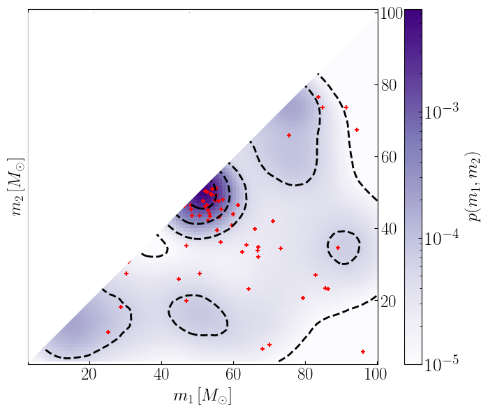
Figure 9: Left: The KDE estimate from data with error for an anticorrelation is added in it. The true distribution is a mixture of a uniform distribution and a bivariate Gaussian with equal and uncorrelated variances in the two dimensions. We then simulate a measurement error which is strongly anticorrelated between the two dimensions to generate mock data parameter samples (see main text for details). We see the contours around (50, 50) is wider (elliptical) and clearly show an anti-correlation. Right: The result after reweighting iteration are applied. We see iterative reweighting reduce the artificial correlation and we do not see elliptical regions around the peaks and results are close to our true distribution.

We here demonstrate iterative reweighted KDE over 2D mock data sets. We start with 60 mock events, 50% from a two-dimensional uniform distribution and 50% from a bi-variate normal (Gaussian) distribution. The normal distribution mean is $\mu=(50,50)$ (in arbitrary units) and we take the two dimensions to be uncorrelated each with a variance of $9$. We added error in our mock data values with an anti-correlation between the two dimensions using covariance $\Sigma_{p}=\bigl{(}\begin{smallmatrix}32.5&-31.5\\ -31.5&32.5\end{smallmatrix}\bigr{)}$, corresponding to an error ellipse with 8:1 axes at $45^{\circ}$, to mimic the anticorrelation between $m_{1}$ and $m_{2}$ along a contour of constant chirp mass. 100 mock parameter samples with the same error covariance are then generated around each measured value. We construct KDE on our errored data points and apply our reweighting scheme. The main idea we want to check if our scheme can reduce this artificial correlation we added in true distribution. The left panel of Fig. 9 is the KDE estimate on errored data before applying iterative reweighting. We can clearly see an anti-correlation we added into our true distribution around the peaks $(50,50)$. The right panel of Fig 9 is the results after we apply our iterative reweighting scheme and use the last 900 iterations to get median curves. We can see that anti-correlation is removed and our method recovered the true distribution. This example shows that our method can reduce effect of artificial correlation in the real data. We also compute 1-d results from these 2-d iterative reweighted average results and compared this corresponding true distribution in 1-d that we expect from true 2-d distribution. Note that our 2-d distribution can be a union of two 1-d uniform distribution with a Gaussian peak $\mu=50$. Fig. 10 shows the true distribution in 1d (black dashed) where the red curves are results of numerical integration of iterative reweighted KDE estimates for the last 900 iterations. The median (solid) red curve matched very closely to the true distribution and recover the peak height and width of Gaussian peak in true distribution.

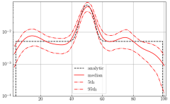
Figure 10: Integrated 1-d component distribution derived from 2-d mock data results. The black dashed curves is the true 1-d distribution composed of uniform and Gaussian components with a Gaussian mean $\mu=50$. The red curved are x coordinate from numerical integration of two dimensional mock data results (as shown on right of Fig. 9) after iterative reweighting is done.

Appendix B Results including GW190814

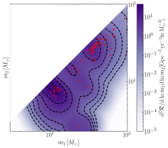
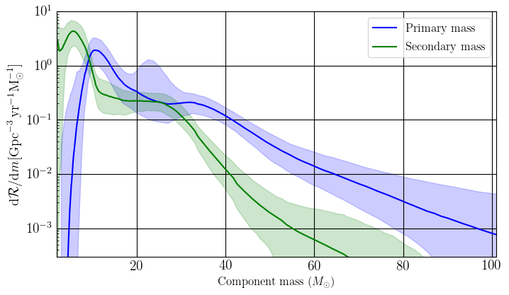
Figure 11: Left: Two dimensional rate estimated with random PE samples for ln $m_{1}$ and ln $m_{2}$ of 70 events (69BBH) and including GW190814 from GWTC-3. The red plus symbols show the median values $m_{1}$ and $m_{2}$ of samples of each event. Right: The corresponding one dimensional component mass distributions from numerical integration of two dimensional results.

In addition to our main results from significant BBH events in GWTC-3, we examine the effect of including the outlier event GW190814 (Abbott et al., 2020b) with low secondary mass $m_{2}=2.59\,M_{\odot}$ $(q=0.112)$. We slightly extend the range of $m_{2}$ over which the KDE is evaluated in order to include the additional event. Fig. 11 summarizes our results, which are also briefly discussed in the main text.

References

- Aasi et al. (2015) Aasi, J., et al. 2015, Class. Quant. Grav., 32, 074001, doi: 10.1088/0264-9381/32/7/074001
- Abbott et al. (2016a) Abbott, B. P., et al. 2016a, Phys. Rev. Lett., 116, 061102, doi: 10.1103/PhysRevLett.116.061102
- Abbott et al. (2016b) —. 2016b, Astrophys. J. Lett., 818, L22, doi: 10.3847/2041-8205/818/2/L22
- Abbott et al. (2019) —. 2019, Phys. Rev. X, 9, 031040, doi: 10.1103/PhysRevX.9.031040
- Abbott et al. (2019) —. 2019, Astrophys. J. Lett., 882, L24, doi: 10.3847/2041-8213/ab3800
- Abbott et al. (2020a) Abbott, R., et al. 2020a. https://arxiv.org/abs/2010.14533
- Abbott et al. (2020b) —. 2020b, Astrophys. J. Lett., 896, L44, doi: 10.3847/2041-8213/ab960f
- Abbott et al. (2021) —. 2021, Phys. Rev. X, 11, 021053, doi: 10.1103/PhysRevX.11.021053
- Abbott et al. (2021a) —. 2021a. https://arxiv.org/abs/2111.03606
- Abbott et al. (2021b) —. 2021b. https://arxiv.org/abs/2108.01045
- Abbott et al. (2023a) —. 2023a, Phys. Rev. X, 13, 011048, doi: 10.1103/PhysRevX.13.011048
- Abbott et al. (2023b) —. 2023b. https://arxiv.org/abs/2302.03676
- Abramson (1982) Abramson, I. S. 1982, The Annals of Statistics, 10, 1217 , doi: 10.1214/aos/1176345986
- Acernese et al. (2015) Acernese, F., et al. 2015, Class. Quant. Grav., 32, 024001, doi: 10.1088/0264-9381/32/2/024001
- Antonini et al. (2023) Antonini, F., Gieles, M., Dosopoulou, F., & Chattopadhyay, D. 2023, MNRAS, 522, 466, doi: 10.1093/mnras/stad972
- Antonini & Rasio (2016) Antonini, F., & Rasio, F. A. 2016, ApJ, 831, 187, doi: 10.3847/0004-637X/831/2/187
- Baibhav et al. (2023) Baibhav, V., Doctor, Z., & Kalogera, V. 2023, Astrophys. J., 946, 50, doi: 10.3847/1538-4357/acbf4c
- Baird et al. (2013) Baird, E., Fairhurst, S., Hannam, M., & Murphy, P. 2013, Phys. Rev. D, 87, 024035, doi: 10.1103/PhysRevD.87.024035
- Banerjee (2021) Banerjee, S. 2021, MNRAS, 503, 3371, doi: 10.1093/mnras/stab591
- Belczynski et al. (2020) Belczynski, K., Klencki, J., Fields, C. E., et al. 2020, A&A, 636, A104, doi: 10.1051/0004-6361/201936528
- Breiman et al. (1977) Breiman, L., Meisel, W., & Purcell, E. 1977, Technometrics, 19, 135. http://www.jstor.org/stable/1268623
- Broekgaarden et al. (2022) Broekgaarden, F. S., Berger, E., Stevenson, S., et al. 2022, MNRAS, 516, 5737, doi: 10.1093/mnras/stac1677
- Callister & Farr (2023) Callister, T. A., & Farr, W. M. 2023. https://arxiv.org/abs/2302.07289
- Callister et al. (2021) Callister, T. A., Haster, C.-J., Ng, K. K. Y., Vitale, S., & Farr, W. M. 2021, Astrophys. J. Lett., 922, L5, doi: 10.3847/2041-8213/ac2ccc
- Chamandy et al. (2012) Chamandy, N., Muralidharan, O., Najmi, A., & Naidu, S. 2012, Estimating Uncertainty for Massive Data Streams, https://research.google/pubs/pub43157/
- Cutler & Flanagan (1994) Cutler, C., & Flanagan, E. E. 1994, Phys. Rev. D, 49, 2658, doi: 10.1103/PhysRevD.49.2658
- Dempster et al. (1977) Dempster, A. P., Laird, N. M., & Rubin, D. B. 1977, Journal of the Royal Statistical Society. Series B (Methodological), 39, 1. http://www.jstor.org/stable/2984875
- Dominik et al. (2015) Dominik, M., Berti, E., O’Shaughnessy, R., et al. 2015, Astrophys. J., 806, 263, doi: 10.1088/0004-637X/806/2/263
- Edelman et al. (2021) Edelman, B., Doctor, Z., Godfrey, J., & Farr, B. 2021. https://arxiv.org/abs/2109.06137
- Edelman et al. (2023) Edelman, B., Farr, B., & Doctor, Z. 2023, Astrophys. J., 946, 16, doi: 10.3847/1538-4357/acb5ed
- Efron (1979) Efron, B. 1979, The Annals of Statistics, 7, 1 . https://doi.org/10.1214/aos/1176344552
- Farah et al. (2023) Farah, A. M., Edelman, B., Zevin, M., et al. 2023. https://arxiv.org/abs/2301.00834
- Fishbach & Holz (2017) Fishbach, M., & Holz, D. E. 2017, Astrophys. J. Lett., 851, L25, doi: 10.3847/2041-8213/aa9bf6
- Fishbach & Holz (2020) —. 2020, Astrophys. J. Lett., 891, L27, doi: 10.3847/2041-8213/ab7247
- Kimball et al. (2021) Kimball, C., et al. 2021, Astrophys. J. Lett., 915, L35, doi: 10.3847/2041-8213/ac0aef
- Kovetz et al. (2017) Kovetz, E. D., Cholis, I., Breysse, P. C., & Kamionkowski, M. 2017, Phys. Rev. D, 95, 103010, doi: 10.1103/PhysRevD.95.103010
- LVK (2021a) LVK. 2021a, GWTC-3: Parameter estimation data release, Zenodo, doi: 10.5281/zenodo.5546663
- LVK (2021b) —. 2021b, GWTC-3: O1+O2+O3 Search Sensitivity Estimates, Zenodo, doi: 10.5281/zenodo.5636816
- Mandel (2010) Mandel, I. 2010, Phys. Rev. D, 81, 084029, doi: 10.1103/PhysRevD.81.084029
- Mandel & de Mink (2016) Mandel, I., & de Mink, S. E. 2016, MNRAS, 458, 2634, doi: 10.1093/mnras/stw379
- Miller et al. (2020) Miller, S., Callister, T. A., & Farr, W. 2020, Astrophys. J., 895, 128, doi: 10.3847/1538-4357/ab80c0
- Ng et al. (2018) Ng, K. K. Y., Vitale, S., Zimmerman, A., et al. 2018, Phys. Rev. D, 98, 083007, doi: 10.1103/PhysRevD.98.083007
- O’Leary et al. (2016) O’Leary, R. M., Meiron, Y., & Kocsis, B. 2016, Astrophys. J. Lett., 824, L12, doi: 10.3847/2041-8205/824/1/L12
- Olejak et al. (2021) Olejak, A., Belczynski, K., & Ivanova, N. 2021, A&A, 651, A100, doi: 10.1051/0004-6361/202140520
- Powell et al. (2019) Powell, J., Stevenson, S., Mandel, I., & Tino, P. 2019, Mon. Not. Roy. Astron. Soc., 488, 3810, doi: 10.1093/mnras/stz1938
- Ray et al. (2023) Ray, A., Magaña Hernandez, I., Mohite, S., Creighton, J., & Kapadia, S. 2023. https://arxiv.org/abs/2304.08046
- Rinaldi & Del Pozzo (2021) Rinaldi, S., & Del Pozzo, W. 2021. https://arxiv.org/abs/2109.05960
- Rodriguez et al. (2016) Rodriguez, C. L., Chatterjee, S., & Rasio, F. A. 2016, Phys. Rev. D, 93, 084029, doi: 10.1103/PhysRevD.93.084029
- Rodriguez et al. (2019) Rodriguez, C. L., Zevin, M., Amaro-Seoane, P., et al. 2019, Phys. Rev. D, 100, 043027, doi: 10.1103/PhysRevD.100.043027
- Sadiq et al. (2022) Sadiq, J., Dent, T., & Wysocki, D. 2022, Phys. Rev. D, 105, 123014, doi: 10.1103/PhysRevD.105.123014
- Sain & Scott (1996) Sain, S. R., & Scott, D. W. 1996, J. Am. Stat. Assoc., 91, 1525. https://www.tandfonline.com/doi/abs/10.1080/01621459.1996.10476720
- Schneider et al. (2023) Schneider, F. R. N., Podsiadlowski, P., & Laplace, E. 2023, Astrophys. J. Lett., 950, L9, doi: 10.3847/2041-8213/acd77a
- Talbot & Thrane (2018) Talbot, C., & Thrane, E. 2018, Astrophys. J., 856, 173, doi: 10.3847/1538-4357/aab34c
- Terrell & Scott (1992) Terrell, G. R., & Scott, D. W. 1992, The Annals of Statistics, 20, 1236 . https://doi.org/10.1214/aos/1176348768
- Thrane & Talbot (2019) Thrane, E., & Talbot, C. 2019, Publ. Astron. Soc. Austral., 36, e010, doi: 10.1017/pasa.2019.2
- Tiwari (2021) Tiwari, V. 2021, Class. Quant. Grav., 38, 155007, doi: 10.1088/1361-6382/ac0b54
- Tiwari (2022) —. 2022, Astrophys. J., 928, 155, doi: 10.3847/1538-4357/ac589a
- Tiwari (2023) —. 2023. https://arxiv.org/abs/2304.03498
- Tiwari & Fairhurst (2021) Tiwari, V., & Fairhurst, S. 2021, Astrophys. J. Lett., 913, L19, doi: 10.3847/2041-8213/abfbe7
- Toubiana et al. (2023) Toubiana, A., Katz, M. L., & Gair, J. R. 2023. https://arxiv.org/abs/2305.08909
- van Son et al. (2022) van Son, L. A. C., de Mink, S. E., Renzo, M., et al. 2022, ApJ, 940, 184, doi: 10.3847/1538-4357/ac9b0a
- Veitch et al. (2015) Veitch, J., et al. 2015, Phys. Rev. D, 91, 042003, doi: 10.1103/PhysRevD.91.042003
- Veske et al. (2021) Veske, D., Bartos, I., Márka, Z., & Márka, S. 2021. https://arxiv.org/abs/2105.13983
- Wang & Wang (2011) Wang, B., & Wang, X. 2011. https://arxiv.org/abs/0709.1616
- Wysocki (2020) Wysocki, D. 2020, Calibrating semi-analytic VT’s to injections in O3a, https://dcc.ligo.org/LIGO-T2000432/public
- Wysocki et al. (2019) Wysocki, D., Lange, J., & O’Shaughnessy, R. 2019, Physical Review D, 100. http://dx.doi.org/10.1103/PhysRevD.100.043012
- Zevin et al. (2021) Zevin, M., Bavera, S. S., Berry, C. P. L., et al. 2021, ApJ, 910, 152, doi: 10.3847/1538-4357/abe40e
- Zevin et al. (2021) Zevin, M., Bavera, S. S., Berry, C. P. L., et al. 2021, Astrophys. J., 910, 152, doi: 10.3847/1538-4357/abe40e