Some remarks on compositeness of $T^{+}_{cc}$

Abstract

Recently LHCb experimental group find an exotic state $T^{+}_{cc}$ from the process $p\bar{p}\to D^{0}D^{0}\pi^{+}+X$. A key question is if it is just a molecule or may have confined tetraquark ingredient. To investigate this, different methods are taken, including two channel ($D^{*+}D^{0}$ and $D^{*0}D^{+}$) $K$-matrix unitarization and single channel Flatté-like parametrization method analysed by pole counting rule and spectral density function sum rule. It demonstrates that $T^{+}_{cc}$ is a molecular state, though the possibility that there may exist elementary ingredient can not be excluded, by rough analysis on its production rate.

1 Introduction

The LHCb collaboration has found a very narrow peak structure named $T^{+}_{cc}$ in the $D^{0}D^{0}\pi^{+}$ invariant mass spectrum, in $pp\to X+D^{0}D^{0}\pi^{+}$ process[1]. The mass parameters obtained from a generic constant-width Breit-Wigner fit are obtained as

$$\delta m_{BW}=-273\pm 61\pm 5^{+11}_{-14}~{}\mathrm{keV}\ ,\,\,\,\Gamma_{BW}=410\pm 165\pm 43^{+18}_{-38}~{}\mathrm{keV}$$

where $\delta m_{BW}$ defines the mass shift with respect to the $D^{*+}D^{0}$ threshold. Later it is suggested that $T^{+}_{cc}$ is more possibly an isoscalar state with spin-parity quantum numbers $J^{P}=1^{+}$[2]. The constituent of $T^{+}_{cc}$ is $cc\bar{u}\bar{d}$ and there is no annihilated quark pair, similar as $X_{1}(2900)$ ($ud\bar{s}\bar{c}$)[3, 4].

The experimental observation has stimulated a lot of theoretical discussions. First of all, there are some dynamical lattice QCD simulations about double charmed tetraquarks, though not providing a definite conclusion on the existence of the $T^{+}_{cc}$ state[5, 6]. Recently, based on (2 + 1)-flavor lattice QCD simulations, $D^{*}D$ system is studied more carefully. It is verified that there is a loosely bound state near threshold (-10 keV) [7]. Many phenomenological studies have also been made. A theoretical prediction is that there may exist a $cc\bar{u}\bar{d}$ tetraquark with $J^{P}=1^{+}$ near $D^{*+}D^{0}$ threshold [8]. Besides, the heavy meson chiral effective field theory (HMChEFT) is used, which considers contact and one pion exchange (OPE) interaction. The analysis prefers that $T^{+}_{cc}$ state is a molecule of $D^{*+}D^{0}$ and $D^{*0}D^{+}$[9, 10]. The effect of triangle diagram singularity is also evaluated with $D^{*}D\pi$ interactions. It is found that the contribution is too weak than that of the tree diagram, which suggests that $T^{+}_{cc}$ is not from triangle singularity [11]. The pole parameters of $T^{+}_{cc}$ extracted from a simple $K$-matrix amplitude are also studied and it is found that $T^{+}_{cc}$ may originate from a $D^{*+}D^{0}$ virtual state [12]. The extended chiral lagrangian with $K$-matrix unitarity approach is also applied, and it is suggested that vector meson exchanges play a crucial role in forming $T^{+}_{cc}$ bound state of $D^{*}D$ [13].

In this work, to estimate that whether $T^{+}_{cc}$ is just a loosely-bound s-wave molecule of $D^{*}D$ or it contains $cc\bar{u}\bar{d}$ ingredient, different approaches are used. Firstly we take the approach similar to that of Ref. [13], using two channel ($D^{*+}D^{0}$ and $D^{*0}D^{+}$) $K$-matrix unitarization with hidden gauge chiral lagrangian. In reference [13], the authors only consider the vector exchanging diagram contributions and there is no experimental data fitting. In this paper, more complete interactions including pseudoscalar, vector exchanges and $D^{*}D$ contact terms are introduced and a combined fit of $DD\pi$, $D\pi$ and $DD$ channels is made. It indicates that the vector meson $\rho$ coupling exchanges really make non-negligible contributions in generating $T^{+}_{cc}$ resonance comparing with other two interactions. In this scheme, there exists a bound state near the $D^{*+}D^{0}$ threshold which suggests that $T^{+}_{cc}$ may be a $D^{*}D$ molecule. Furthermore, the Flatté-like parametrization is also used. Through a combined fit on three-body and two-body invariant mass spectrum, we find that the result is same based on PCR and spectral density function sum rule calculation[14, 15, 16, 17, 18, 19]: there is only one pole near $D^{*}D$ threshold and the corresponding $\mathcal{Z}\simeq 1$. We also try to judge the compositeness of $T^{+}_{cc}$ by comparing its productivity ($pp\to T^{+}_{cc}+X$) with different theoretical estimations. The $D^{*}D$ molecule productivity should be significantly less than a confined tetraquark productivity[20]. However, according to a rough comparison with $\Xi_{cc}$ data, the order of magnitude of $T^{+}_{cc}$ production rate is in between, hence it is also hard to make a judgement.

This paper is as follows: Sec. I is the introduction, in Sec. II, the traditional K-matrix unitarization approach with hidden gauge chiral lagrangian in $s$-wave approximation is introduced and its numerical fit is shown. In Sec. III, other frameworks are employed to analyse the compositeness of $T^{+}_{cc}$. Finally, in Sec. IV, a brief conclusion on the structure of $T^{+}_{cc}$ is made.

2 K-matrix unitarity approach

A chiral lagrangian with hidden gauge symmetry is often used to describe vector and pseudoscalar meson interactions[21, 22, 23, 24]. Here we list relevant coupling terms

$$\mathcal{L}=\mathcal{L}_{0}-ig\mathrm{Tr}([P,\partial_{\mu}P]V^{\mu})+ig\mathrm{Tr}([V^{\nu},\partial_{\mu}V_{\nu}]V^{\mu})$$ (1)

$$-\frac{g^{2}}{2}\mathrm{Tr}([P,V_{\mu}]^{2})+\frac{g^{2}}{4}\mathrm{Tr}([V_{\mu},V_{\nu}]^{2})\ ,$$

where $\mathcal{L}_{0}$ is the free lagrangian for pseudoscalar and vector mesons. P and V denote, respectively, properly normalized pseudoscalar and vector meson matrices

$$P=\begin{pmatrix}\frac{\eta}{\sqrt{3}}+\frac{\eta^{\prime}}{\sqrt{6}}+\frac{\pi^{0}}{\sqrt{2}}&\pi^{+}&K^{+}&\bar{D}^{0}\\ \pi^{-}&\frac{\eta}{\sqrt{3}}+\frac{\eta^{\prime}}{\sqrt{6}}-\frac{\pi^{0}}{\sqrt{2}}&K^{0}&D^{-}\\ K^{-}&\bar{K}^{0}&-\frac{\eta}{\sqrt{3}}+\sqrt{\frac{2}{3}}\eta^{\prime}&D^{-}_{s}\\ D^{0}&D^{+}&D^{+}_{s}&\eta_{c}\end{pmatrix}\ ,$$ (2)

$$V=\begin{pmatrix}\frac{\omega}{\sqrt{2}}+\frac{\rho^{0}}{\sqrt{2}}&\rho^{+}&K^{*+}&\bar{D}^{*0}\\ \rho^{-}&\frac{\omega}{\sqrt{2}}-\frac{\rho^{0}}{\sqrt{2}}&K^{*0}&D^{*-}\\ K^{*-}&\bar{K}^{*0}&\phi&D^{*-}_{s}\\ D^{*0}&D^{*+}&D^{*+}_{s}&J/\psi\end{pmatrix}\ .$$ (3)

It needs to point out that, only $SU(2)$ symmetry really holds. That is all couplings constants, appearing in vertices of PPV, VVV and PPVV types, are invariable in isospin space. Different vertices (including $s$ and $c$) should be considered case by case. We also adopt previous theoretical work to estimate these coupling constants.

From Eq. (1), we can get the contact, $t$ and $u$ channel diagrams about $D^{*+}D^{0}\to D^{*0}D^{+}$ process. We list their amplitudes successively. First is contact diagrams,

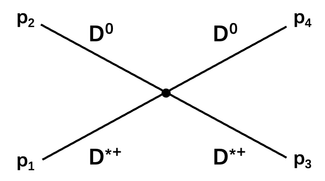
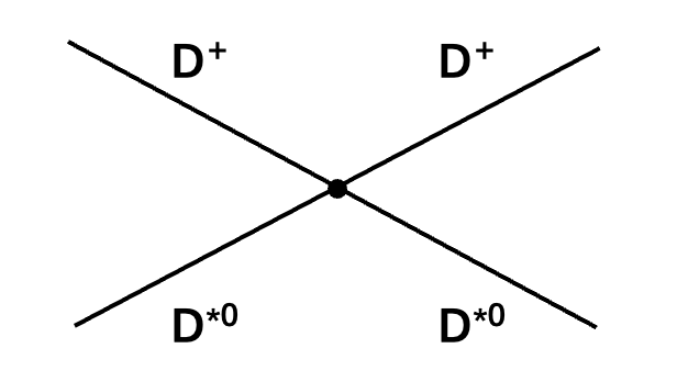
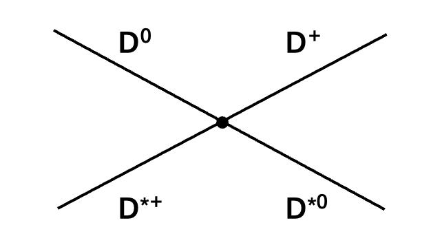
Figure 1: Contact diagrams.

$$iM^{c}_{ij}=i~{}g_{D^{*}DD^{*}D}^{2},$$ (4)

where $i,j=1,2$ refer to $D^{*+}D^{0}$ and $D^{*0}D^{+}$ channel, respectively. The coupling $g_{4D}$ has been estimated when studying $X(3872)$ [17], that $g(=g_{D^{*}DD^{*}D})\simeq 16$.

The $t$ channel diagrams include vector meson ($J/\psi$ or $\rho$, $\omega$) exchanges [13]. We also neglect the momentum dependence in the denominator of the propagator near the threshold. Here an estimation about coupling constants from the PPV and VVV vertices are given. That is when $i,j=1,1$ or $2,2$, the coupling constant $g(=g_{J/\psi D^{(*)}D^{(*)}})\simeq 7.7$, and when $i,j=1,2$ or $2,1$, $g(=g_{\rho D^{(*)}D^{(*)}})\simeq 3.9$, Which is obtained from the vector meson dominance (VMD) assumption [22]. The $t$ channel amplitudes are hence written as follows (Fig. 2),

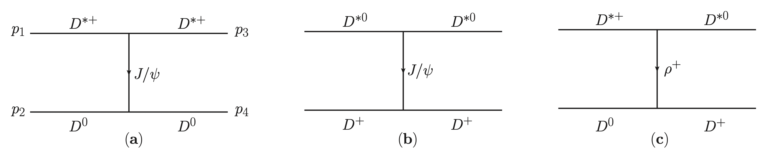
Figure 2: The $t$ channel diagrams.

$$iM^{t}_{ij}=iD_{ij}(p_{1}+p_{3})\cdot(p_{2}+p_{4})~{}\epsilon(p_{1})\cdot\epsilon^{*}(p_{3}),$$ (5)

where

$$D_{ij}=\begin{pmatrix}\frac{g^{2}_{J/\psi D^{(*)}D^{(*)}}}{M^{2}_{J/\psi}}&\frac{g^{2}_{\rho D^{(*)}D^{(*)}}}{m^{2}_{\rho}}\\ \frac{g^{2}_{\rho D^{(*)}D^{(*)}}}{m^{2}_{\rho}}&\frac{g^{2}_{J/\psi D^{(*)}D^{(*)}}}{M^{2}_{J/\psi}}\\ \end{pmatrix}_{ij}.$$ (6)

The third type is $u$ channel diagrams with $\pi$ exchanges as in Fig. 3,

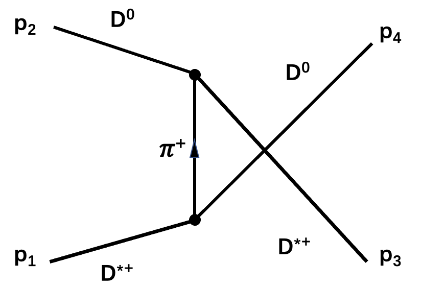
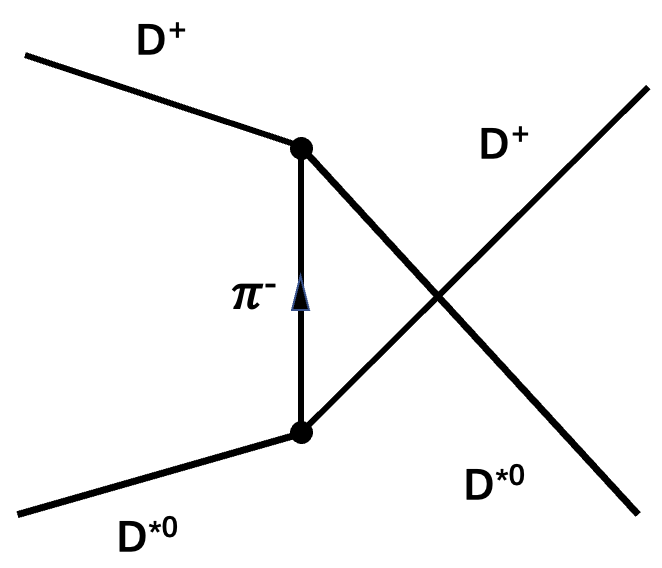
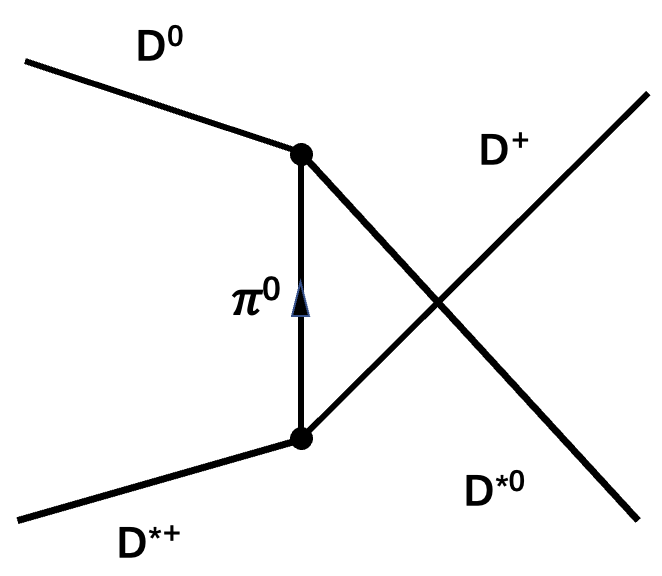
Figure 3: The $u$ channel diagrams.

and the amplitudes are

$$iM^{u}_{ij}=iE_{ij}g_{\pi DD^{*}}^{2}\frac{\epsilon(p_{1})\cdot(p_{1}-2p_{4})~{}\epsilon^{*}(p_{3})\cdot(p_{3}-2p_{2})}{(p_{1}-p_{4})^{2}-m_{\pi}^{2}},$$ (7)

where

$$E_{ij}=\begin{pmatrix}-1&\frac{1}{2}\\ \frac{1}{2}&-1\\ \end{pmatrix}_{ij}.$$ (8)

The coupling strength $g_{\pi DD^{*}}$ can be restricted by the decay process $D^{*+}\to D^{0}\pi^{+}$, and we take the value $g(=g_{\pi DD^{*}})\simeq 8.4$ [25]. There also exist $u$ channel diagrams with pseudo-scalar meson $\eta_{c}$ exchanges. They are not important at this energy range as tested numerically, so we neglect these diagrams. As for the amplitudes corresponding to Fig. 3, the $u$ channel exchanging $\pi$ is somewhat special because it is possible to exchange one on-shell $\pi$ meson. After partial wave projection, there exists, in tree level amplitudes, an additional cut in the energy region above $D^{*+}D^{0}$ threshold. Here this singularity will disturb unitarity. To remedy this, we keep the relation $m_{D^{*}}=m_{D}+m_{\pi}$ to keep away from the singularity, similar to Refs. [9, 10]. At last, we get the total couple channel amplitudes

$$M_{ij}=M^{c}_{ij}+M^{t}_{ij}+M^{u}_{ij}\ .$$ (9)

Furthermore, it can be unitized by the relation

$$\mathbf{T}^{-1}=\mathbf{K}^{-1}-\mathbf{g}(s),$$ (10)

where $\mathbf{T}$ is the unitarized scattering $T$ matrix, $\mathbf{K}$ is a two channel scattering amplitude matrix in s-wave approximation [26]. And $\mathbf{g}(s)\equiv\mathrm{diag}\{g_{i}(s)\}$. In our normalization

$$g_{i}(s;M_{i},m_{i})=-16\pi i\int\frac{d^{4}q}{(2\pi)^{4}}\frac{1}{(q^{2}-M_{i}^{2}+i\epsilon)((P-q)^{2}-m_{i}^{2}+i\epsilon)},\,\,(s=P^{2})$$ (11)

where $M_{i}$ is the vector meson mass and $m_{i}$ the pseudoscalar meson mass in the $i$-th channel. The expression of $g_{i}(s)$ in Eq. (11) is renormalized using standard $\overline{\mathrm{MS}}$ scheme, which introduces an explicit renormalization scale ($\mu$) dependence. In our fit we choose the same $\mu$ parameter in two channels.

To get a finite width for the $T_{cc}^{+}$ state below $D^{*}D$ threshold we need to consider the finite width of the $D^{*}$ state. This is accomplished by performing a convolution of the $g_{i}(s)$ functions with the mass distribution of the $D^{*}$ states [27]:

$$S\left(s_{V};M_{V},\Gamma_{V}\right)\equiv-\frac{1}{\pi}\operatorname{Im}\left\{\frac{1}{s_{V}-M_{V}^{2}+iM_{V}\Gamma_{V}}\right\}$$ (12)

such that

$$\tilde{g}_{i}(s;M_{i},m_{i})=\mathcal{C}\int_{s_{Vmin}}^{s_{Vmax}}ds_{V}g_{i}(s;\sqrt{s_{V}},m_{i})S\left(s_{V};M_{i},\Gamma_{i}\right)\ ,$$ (13)

where $\mathcal{C}$ is a normalization factor. The main contribution to this integration is from the region around the unstable mass $s_{V}\sim M_{V}^{2}$, so we can introduce a cutoff $s_{Vmin}$ and $s_{Vmax}$. For example, for $\tilde{g}_{1}$ it is integrated from $(m_{D_{0}}+m_{\pi^{+}})^{2}$ to $(m_{D^{*+}}+2\Gamma_{D^{*+}})^{2}$ and for $\tilde{g}_{2}$ it is integrated from $(m_{D_{0}}+m_{\pi^{0}})^{2}$ to $(m_{D^{*0}}+2\Gamma_{D^{*0}})^{2}$. Here we take the decay widths as constants because we only focus on the region near the $D^{*+}D^{0}$ threshold and it makes little difference neglecting the $s$ dependence in numerical calculations. The constant decay widths suggested by PDG [28] read

$$\Gamma_{D^{*+}}=83.4~{}\mathrm{keV},~{}~{}\Gamma_{D^{*0}}=55.3~{}\mathrm{keV}.$$ (14)

In order to fit the final state three-body invariant mass spectrum of $D^{0}D^{0}\pi^{+}$, the final-state interaction (FSI) [19] between $D^{*+}D^{0}$ and/or $D^{*0}D^{+}$ needs to be considered, before considering the $D^{*+}\to D^{0}+\pi^{+}$ decay. The FSI amplitude reads

$$\mathcal{F}_{D^{*+}D^{0}}(s)=\alpha_{1}~{}T_{11}+\alpha_{2}~{}T_{21}\ ,$$ (15)

where $\alpha_{1}$, $\alpha_{2}$ are smooth real polynomials, and since the energy region of interest is very small, we treat them as constant parameters near the thresholds of $D^{*+}D^{0}$ and $D^{*0}D^{+}$. Finally, the decay of $T^{+}_{cc}\to D^{0}D^{0}\pi^{+}$ can therefore be expressed as in Fig. 4. And the final scattering amplitude is written as

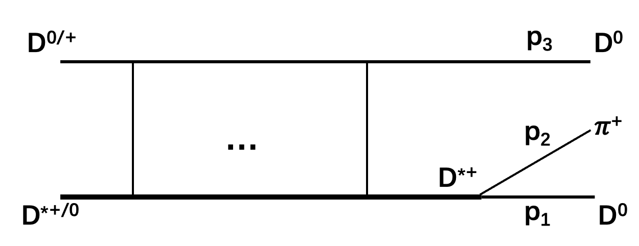
Figure 4: The process of $T^{+}_{cc}\to D^{0}D^{0}\pi^{+}$.

$$t= \mathcal{F}_{D^{*+}D^{0}}\left[\frac{{\epsilon}\cdot[({p}_{1}-{p}_{2})+\frac{m_{\pi^{+}}^{2}-m_{D^{0}}^{2}}{m_{D^{*+}}^{2}}({p}_{1}+{p}_{2})]}{M_{12}^{2}-m_{D^{*+}}^{2}+iM_{12}\Gamma_{D^{*+}}(M_{12})}\right.$$ (16)

$$\left.+\frac{{\epsilon}\cdot[({p}_{3}-{p}_{2})+\frac{m_{\pi^{+}}^{2}-m_{D^{0}}^{2}}{m_{D^{*+}}^{2}}({p}_{3}+{p}_{2})]}{M_{23}^{2}-m_{D^{*+}}^{2}+iM_{23}\Gamma_{D^{*+}}(M_{23})}\right].$$

where $M_{12}$ and $M_{23}$ are Dalitz kinematic variables of the final three-body state. The corresponding definition is $M_{ij}^{2}=(p_{i}+p_{j})^{2}$, and ${\epsilon}={\epsilon}(P)$ corresponds to the polarization vector of $T^{+}_{cc}$, $P=\left(p_{1}+p_{2}+p_{3}\right)$, $P^{2}=s$. These invariants have the relation that $M^{2}_{12}+M^{2}_{13}+M^{2}_{23}=P^{2}+p_{1}^{2}+p_{2}^{2}+p_{3}^{2}$. Finally the decay width of $T_{cc}^{+}$ is given by

$$d\Gamma(\sqrt{s})=\frac{\mathcal{N}}{2}\frac{32}{\pi}\frac{1}{s^{3/2}}|t|^{2}ds_{12}ds_{23}.$$ (17)

The factor $\frac{1}{2}$ in the above equation comes from averaging the two integrals of $D^{0}$ in the final state. In order to fit the experimental data, the normalization factor $\mathcal{N}$ should be introduced. As for the two FSI parameters, $\alpha_{1}$ can be absorbed in the coefficients $\mathcal{N}$. So $\alpha_{1}=1$ is fixed and there remains one free parameter $\alpha_{2}$. Besides, when we get the yields for the $D^{0}D^{0}\pi^{+}$ invariant mass spectrum, the resolution function is convoluted

$$\mathrm{Yields}(l)=\int_{l-2\sigma}^{l+2\sigma}dl^{\prime}\frac{1}{\sqrt{2\pi}\sigma}\Gamma\left(l^{\prime}\right)\mathrm{e}^{-\frac{\left(l^{\prime}-l\right)^{2}}{2\sigma^{2}}},$$ (18)

where $\sigma=1.05\times 263\mathrm{keV}$ [1]. At last, invariant mass distributions for the selected two body (particles 2 and 3 for example) can also be derived as the the following function

$$\frac{dBr}{dm_{23}}=\mathcal{N}^{\prime}\int_{m^{2}_{D^{0}D^{0}\pi^{+}}}^{m_{max}^{2}}ds\int ds_{12}|t(s,s_{12},s_{23})|^{2}$$ (19)

where $\mathcal{N}^{\prime}$ is another normalization constant, $m_{23}$ is the invariant mass of particles 2 and 3. The $T^{+}_{cc}$ energy is integrated from the initial energy $m_{D^{0}D^{0}\pi^{+}}$ to a cutoff $m_{max}$.

Data obtained from LHCb collaboration about three body final states $D^{0}D^{0}\pi^{+}$[1] and two body invariant mass distributions $D^{0}\pi^{+}$, $D^{0}D^{0}$ and $D^{+}D^{0}$[2] are used to make a combined fit. The normalization $\mathcal{N}$, $\mathcal{N^{\prime}}$, FSI parameter $\alpha_{2}$ and renormalization scale $\mu$ are regarded as fit parameters and all coupling constants found in the literature are regarded as fixed parameters (Scheme I).

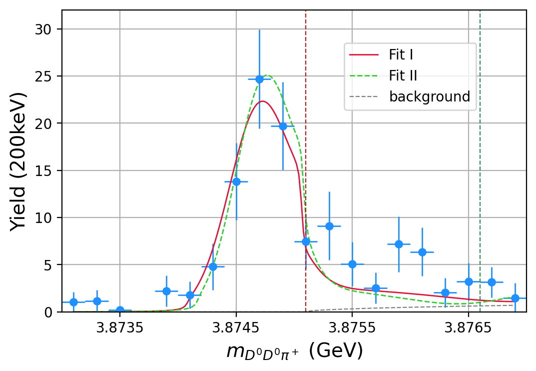
Figure 5: $D^{0}D^{0}\pi^{+}$ final state invariant mass spectrum. The vertical purple dash line indicates the $D^{*+}D^{0}$ threshold and the green one corresponds to the $D^{*0}D^{+}$ threshold. Data come from Ref. [1].

See Fig. 5 for the fit (Scheme I). It is shown that the fit result is very sensitive to the parameter $\mu$. That is because the peak ($T^{+}_{cc}$ state) is too narrow, considering that unit of $\mu$ is GeV but the signal range is in MeV. The discussion above seems to suggest that the fit result prefers a particular choice of parameter $\mu$. This looks annoying but is not actually a physical problem. That is because in the fit we have fixed all coupling strength constants previously determined. To avoid the problem, we can for example take scheme II that all coupling parameters are regarded as fit parameter, and $\mu$ is removed by replacing $g_{i}(s;M_{i},m_{i})$ as $i\rho_{i}(s;M_{i},m_{i})$ (i.e., on shell approximation). The expression $\rho_{i}(s;M_{i},m_{i})$ is the two-body phase space factor

$$\rho_{i}(s;M_{i},m_{i})=\frac{\sqrt{s-(M_{i}+m_{i})^{2}}\sqrt{s-(M_{i}-m_{i})^{2}}}{s}.$$ (20)

The result is that it can still fit well, just that the coupling $g_{\rho DD}$ becomes larger, see Table 1.

The pole location on the $s$-plane is also studied. If $D^{*}$ is taken as a stable particle, Then $T_{cc}^{+}$ appear as a bound state pole located at $\sqrt{s}=3.8746$, i.e., about $500$keV below $D^{*+}D^{0}$ threshold ($\sqrt{s}=3.8751$). Since there is no nearby accompanying virtual pole, we conclude that, according to the pole counting rule (PCR), $T^{+}_{cc}$ is a pure moleclue composed of $DD^{*}$. However, due to the instability of $D^{*}$, the $D^{*}D$ channel opens at the energy a little bit smaller than $m_{D^{*}}+m_{D}$ and the decay of $T_{cc}^{+}$ take place [13].

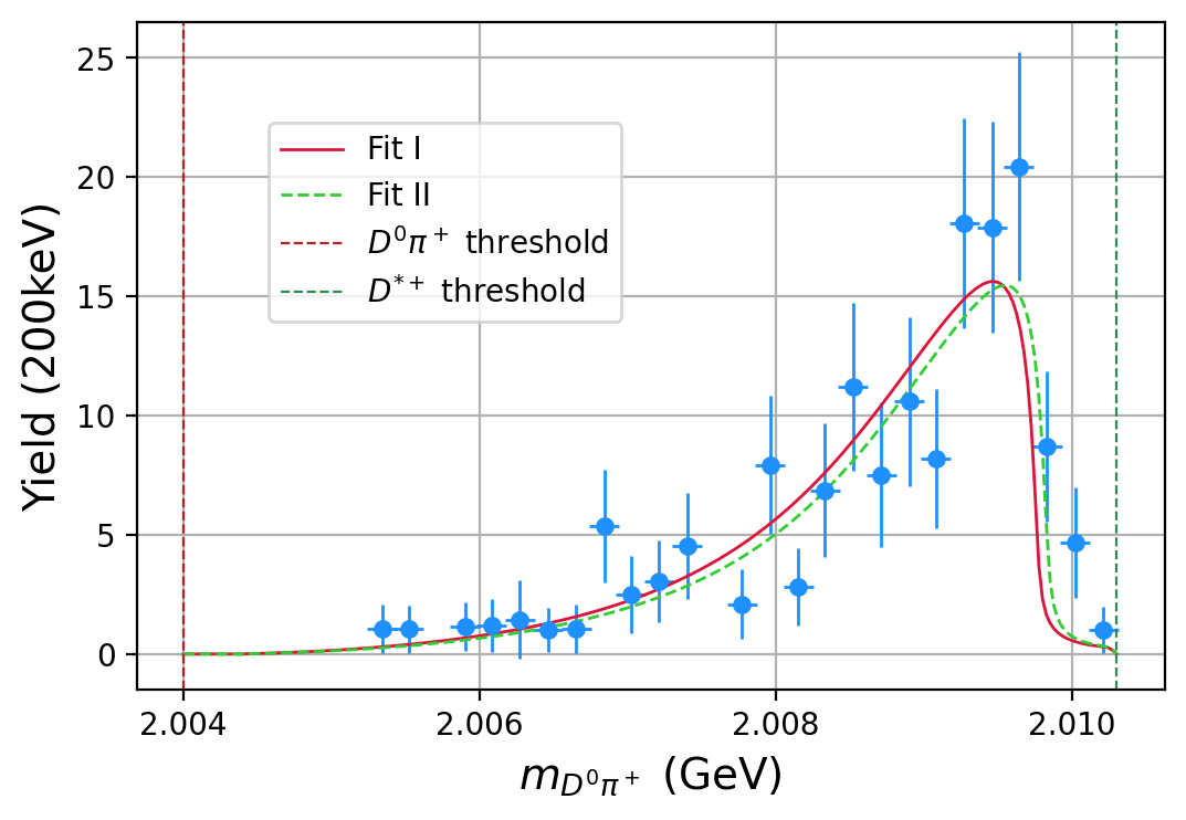
Figure 6: The $D^{0}\pi^{+}$ invariant mass spectrum from three body final state $D^{0}D^{0}+X$ (Data from Ref. [2]).

Furthermore, invariant mass distributions for any two of three final state particles are also taken into consideration. As for $D^{0}\pi^{+}$ state, which comes from $D^{*+}D^{0}$, we take $m_{max}=3.8751\mathrm{GeV}$ and it implies only $T^{+}_{cc}$ below $D^{*+}D^{0}$ threshold make sense to decay into $D^{0}\pi^{+}$ (normalization constant $\mathcal{N}^{\prime}=\mathcal{N_{D\pi}}$).

As for $D^{0}D^{0}$ and $D^{+}D^{0}$ two-body final states, we take the same $m_{max}=3.8751\mathrm{GeV}$ ($\mathcal{N}^{\prime}=\mathcal{N_{DD}}$ here). On the other side, the $D^{+}D^{0}$ final state, which comes from the $D^{+}D^{0}\pi^{0}$ final state, is different. Since $D^{+}D^{0}$ state may come from two channels, $D^{*+}D^{0}$ and $D^{*0}D^{+}$, they need to be considered altogether aided by isospin symmetry. Since the threshold of second channel is higher, we take $m_{max}=3.8766\mathrm{GeV}$, and on account of a symmetry factor $\frac{1}{2}$ in channel including $D^{0}D^{0}$, the normalization constant here is doubled ($\mathcal{N}^{\prime}=2\mathcal{N_{DD}}$). The fitting results are plotted in Fig. 7. Both invariant mass spectrums ($D^{0}D^{0}$and $D^{+}D^{0}$) are with an incoherent background component, parameterised as a product of two-body phase space function $\Phi_{DD}$ and a linear function. For $D^{+}D^{0}$ from channel $T^{+}_{cc}\to D^{*0}D^{+}\to D^{+}D^{0}\pi^{0}/D^{+}D^{0}\gamma$, because the decay channel $D^{*0}\to D^{0}\gamma$ accounts for 35% of total $D^{*0}$ decay width, this incoherent background contribution is non-negligible and needs to be counted specially. Here we take this estimation from Ref. [2] directly.

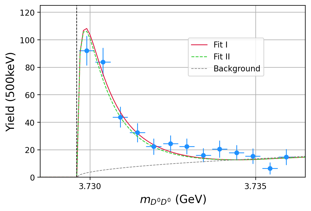
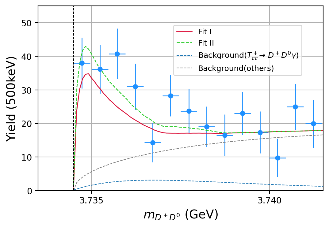
Figure 7: $D^{0}D^{0}$ ($D^{+}D^{0}$) invariant mass spectrum from three body final state $D^{0}D^{0}+X$ ($D^{+}D^{0}+X$) [2], where the vertical line of dashes show $D^{0}D^{0}$ ($D^{+}D^{0}$) threshold.

Finally, the fit parameters are listed in Table 1.

Table 1: Parameters.

Scheme	I	II
$\chi^{2}/d.o.f$	1.16	1.06
$\alpha_{2}$	$-0.43\pm 0.10$	$-0.48\pm 0.13$
$\mu/\mathrm{GeV}$	$1.122\pm 0.001$	–
$g_{D^{*}DD^{*}D}$	fixed=$16$ [17]	$16.0\pm 7.36$
$g_{\pi DD^{*}}$	fixed=$8.4$ [25]	$8.4\pm 6.51$
$g_{\rho D^{(*)}D^{(*)}}$	fixed=$3.9$ [22]	$7.78\pm 1.46$
$g_{J/\psi D^{(*)}D^{(*)}}$	fixed=$7.7$ [22]	$13.8\pm 9.16$

3 Other insights on $T^{+}_{cc}$

In this section, the production of $T^{+}_{cc}$ in some other methods are also analysed to figure out its compositeness. First of all, a single channel Flatté-like parametrization is used. Like the previous calculation in Sec. II, this process is regarded as a cascade decay. The propagator of $T^{+}_{cc}$ is approximated by Flatté form. The later propagator of $D^{*}$ here can only take an simple Breit–Wigner amplitude form, because the energy of this process is near the threshold of $D^{*}D$ and its range is small enough. Besides, the momentum dependent polynomial in the numerator is also normalized by a constant factor $\mathcal{N}$ for convenience. Numerical calculations indicate that these approximation can make little difference.

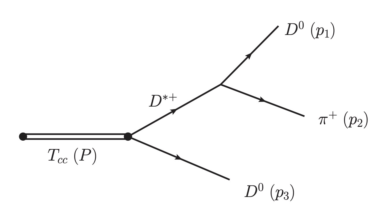
Figure 8: Cascade decay

The total s-wave approximation amplitude about process $T^{+}_{cc}\to D^{0}D^{0}\pi^{+}$ can be written as

$$t= \frac{1}{s-M^{2}+iM\left(g\rho(s)\right)}\times$$ (21)

$$\left(\frac{1}{M_{12}^{2}-m_{D^{*+}}^{2}+iM_{12}\Gamma_{D^{*+}}}+\frac{1}{M_{23}^{2}-m_{D^{*+}}^{2}+iM_{23}\Gamma_{D^{*+}}}\right),$$

where $g$ presents the coupling strength with only channel $D^{*}D$. The doubling of the kinetic variables of the $D^{*}$ propagator is due to the indistinguishability of $D\pi$ in three-body final state, and the symmetry factor $\frac{1}{2}$ is absorbed by the total normalization $\mathcal{N}$. By this parametrization, we make the energy resolution convolution as before and fit the three-body decay width and two-body invarint mass spectrum at the same time using previous Eqs. (17, 19). It is worth pointing out that under normal conditions it will form a divergent peak because of the zero partial decay width. But if we regard $D^{*}$ as an unstable particle, in other words the amplitude can emerge imaginary part when the energy does not reach the $D^{*}D$ threshold yet, the peak is not divergent anymore. We can use the same trick as Eq. (13) to treat $\rho$ in Eq. (21), or more simply take the value $m_{D^{*}}$ in $\rho$ with a imaginary part $\Gamma_{D^{*}}$. The choice of them does not effect the result except for the goodness of fit. Here we take the latter scenario. The united fits result is following.

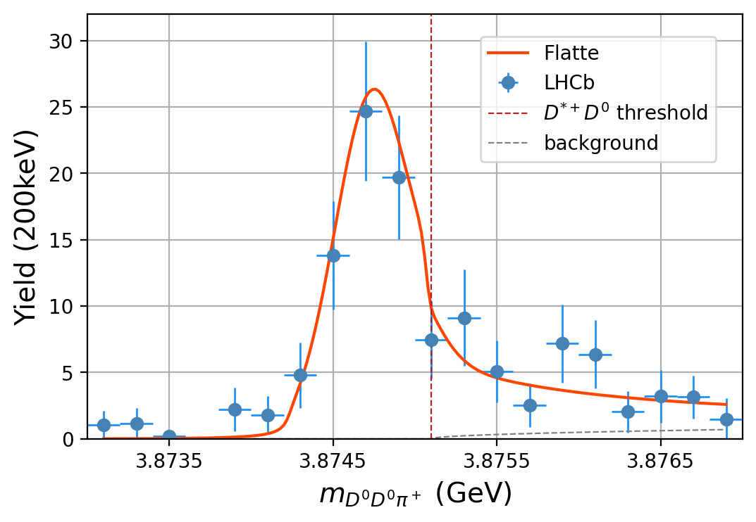
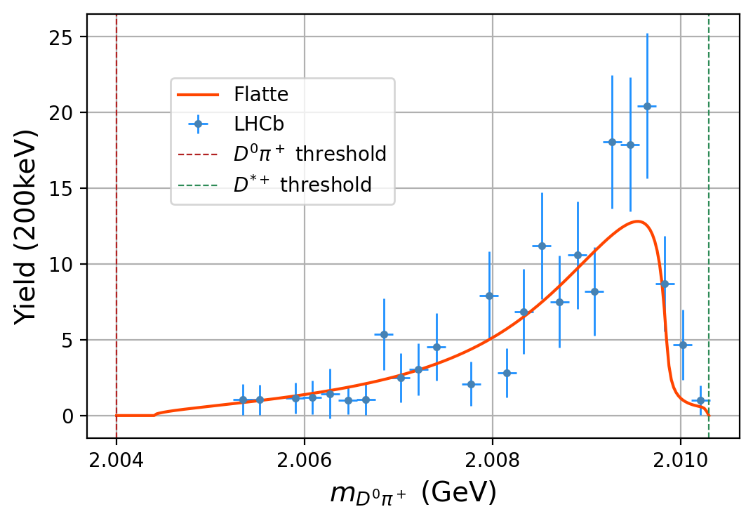
Figure 9: The three-body and two-body invarint mass spectrum

We list the corresponding parameters in Table 2, and the pole structure of the Flatté amplitude is drawn in Fig. 10.

Table 2: Fit parameter

$\chi^{2}/d.o.f$	$g$	$M$
$0.81$ keV	$0.075\pm 0.015$	$3874.1\pm 0.2$MeV

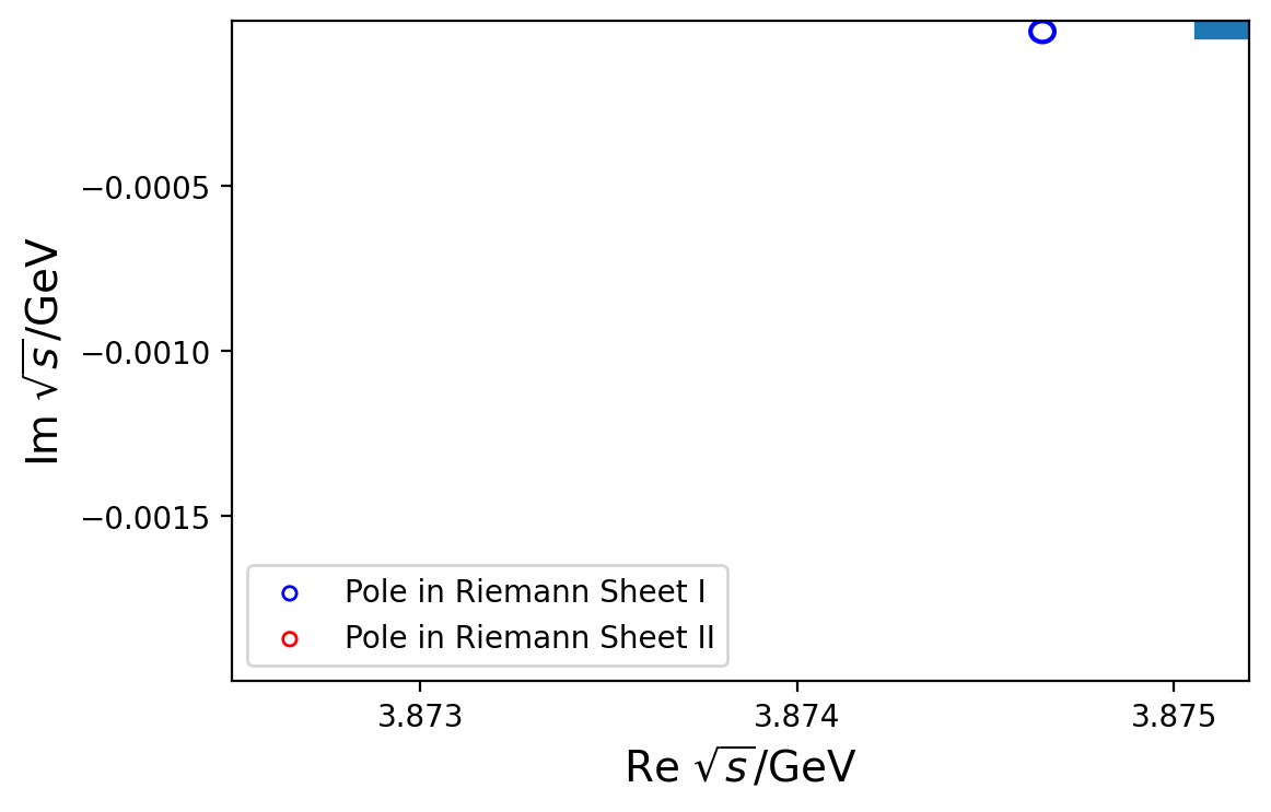
Figure 10: The pole structure of flatté amplitude

Furthermore, according to the Flatté-like parametrization, it is nature to calculate the probability of finding an ‘elementary’ state in the continuous spectrum by the spectral density function[29]

$$\omega(E)=\frac{1}{2\pi}\frac{\tilde{g}\sqrt{2\tilde{M}E}\theta(E)+\tilde{\Gamma}_{0}}{\left|E-E_{f}+\frac{\mathrm{i}}{2}\tilde{g}\sqrt{2\tilde{M}E}+\frac{\mathrm{i}}{2}\tilde{\Gamma}_{0}\right|^{2}},$$ (22)

where $E=\sqrt{s}-m_{D^{*}D}$, $E_{f}=M-m_{D^{*}D}$, $\tilde{M}$ is the reduced mass of $D^{*}D$, $\theta$ is the step function at threshold and $\tilde{\Gamma}_{0}$ is the constant partial width for the remaining couplings. By integrating it with a cut off (usually comparable to the total decay width$\sim\Gamma$), the possibility of finding an ‘elementary’ state in the final state is

$$\mathcal{Z}=\int_{E_{\min}}^{E_{\max}}\omega(E)\mathrm{d}E.$$ (23)

Considering that there is no other channels coupling with $T^{+}_{cc}$ under the $D^{*}D$ threshold, the $\tilde{\Gamma}_{0}$ here should be set zero. In this case, the integrating results in different sections are as follows.

Table 3: Spectral density function integrating $\mathcal{Z}$

$[M-\Gamma,M+\Gamma]$	$[M-2\Gamma,M+2\Gamma]$	$[M-3\Gamma,M+3\Gamma]$
$\sim$ 0	$\sim$ 0	0.01

The result suggests that in a simple single channel Flatté-like parametrization framework, $T^{+}_{cc}$ is a pure molecular state. This is in agreement with the result of Ref. [30], obtained using effective range expansion approximation. Our result is much more definite than that obtained in Ref. [2].

Furthermore, there are also discussions on the compositeness from the production rate of a particle. There is a cross section relation between confined state $\Xi_{cc}$($ccu/ccd$)[31] and $T^{+}_{cc}$. These two experimental data are all collected after 2016, and they are from the same experimental condition, like transverse momentum truncation $p_{T}$ and luminance $9fb^{-1}$. After taking the detection efficiency and branching fractions difference[32], there is a rough relation that

$$\frac{\sigma(pp\to T^{+}_{cc})}{\sigma(pp\to\Xi_{cc})}\sim\frac{1}{3}\times\frac{1}{10}.$$ (24)

If we agree that there exists a universal relation between $(Q/QQ)q$ and $(Q/QQ)qq$ productivity in high energy collision[33], where $Q$ represents heavy quark and $q$ is light quark, we can get a factor $1/3$, which means catching two light quarks are always more difficult, i.e., $\sigma(pp\to\Xi_{cc})\simeq 3\sigma(pp\to(cc\bar{u}\bar{d}))$. So the ratio between observed $T^{+}_{cc}$ and hypothetical tetraquark cross section is derived

$$\frac{\sigma(pp\to T^{+}_{cc})}{\sigma(pp\to(cc\bar{u}\bar{d}))}\sim\frac{1}{10}.$$ (25)

On the other hand, it is natural to estimate the different theoretical cross section orders between ‘elementary’ and ‘molecular’ picture of $T^{+}_{cc}$. Thanks to that $X(3872)$ resonance has analogous characteristics [34, 35](e.g., binding energy and double c quark), there have been some comparisons about these orders of magnitude on $X(3872)$[36, 20]. One can borrow the discussions here and it can be estimated that roughly for $T^{+}_{cc}$

$$\frac{\sigma(pp\to(c\bar{u})(c\bar{d}))}{\sigma(pp\to(cc\bar{u}\bar{d}))}\sim\mathcal{O}(10^{-2})-\mathcal{O}(10^{-3}).$$ (26)

By comparing Eq. (25) and Eq. (26), the productivity of $T^{+}_{cc}$ just falls in between two different cases. So using the productivity argurement does not provide a clear conclusion on the nature of $T^{+}_{cc}$. On the contrary, the analysis provided in this paper, e.g., Table 3 clearly indicates the molecular nature of $T^{+}_{cc}$.

4 Summary

In this work, we study the nature of $T^{+}_{cc}$ by different methods. We use the extended hidden local chiral lagrangian with two channel ($D^{*+}D^{0}$ and $D^{*0}D^{+}$) $K$-matrix approach to describe the process $T^{+}_{cc}\to D^{0}D^{0}\pi^{+}$. The three-body and two-body invariant mass spectrum can be fitted well at the same time. Also the numerical fit results reveal that the vector meson exchanges is more important comparing with $\pi$ exchanges and contact interactions. We also use Flattè formula to study the problem. We conclude that $T^{+}_{cc}$ is definitely a pure molecular state composed of $D^{*}D$, in agreement with many of the results found in the literature, but on a much more confident level.

$Acknowledgements:$ We would like to thank Hao Chen for a careful reading of the manuscript and very helpful discussions. At last, This work is supported in part by National Nature Science Foundations of China under Contract Numbers 11975028.

- [1] LHCb, R. Aaij et al., Nature Phys. 18, 751 (2022).
- [2] LHCb, R. Aaij et al., Nature Commun. 13, 3351 (2022).
- [3] LHCb, R. Aaij et al., Phys. Rev. D 102, 112003 (2020).
- [4] H. Chen, H.-R. Qi, and H.-Q. Zheng, Eur. Phys. J. C 81, 812 (2021).
- [5] Y. Ikeda et al., Phys. Lett. B 729, 85 (2014).
- [6] P. Junnarkar, N. Mathur, and M. Padmanath, Phys. Rev. D 99, 034507 (2019).
- [7] Y. Lyu et al., (2023), arXiv: 2302.04505.
- [8] M. Karliner and J. L. Rosner, Phys. Rev. Lett. 119, 202001 (2017).
- [9] M.-L. Du et al., Phys. Rev. D 105, 014024 (2022).
- [10] Z.-Y. Lin, J.-B. Cheng, and S.-L. Zhu, (2022), arXiv: 2205.14628.
- [11] N. N. Achasov and G. N. Shestakov, Phys. Rev. D 105, 096038 (2022).
- [12] L.-Y. Dai, X. Sun, X.-W. Kang, A. P. Szczepaniak, and J.-S. Yu, Phys. Rev. D 105, L051507 (2022).
- [13] A. Feijoo, W. H. Liang, and E. Oset, Phys. Rev. D 104, 114015 (2021).
- [14] Y. Lu, C. Chen, K.-G. Kang, G.-y. Qin, and H.-Q. Zheng, (2023), arXiv: 2302.04150.
- [15] C. Chen, H. Chen, W.-Q. Niu, and H.-Q. Zheng, Eur. Phys. J. C 83, 52 (2023).
- [16] Q.-R. Gong et al., Phys. Rev. D 94, 114019 (2016).
- [17] C. Meng, J. J. Sanz-Cillero, M. Shi, D.-L. Yao, and H.-Q. Zheng, Phys. Rev. D 92, 034020 (2015).
- [18] O. Zhang, C. Meng, and H. Q. Zheng, Phys. Lett. B 680, 453 (2009).
- [19] D.-L. Yao, L.-Y. Dai, H.-Q. Zheng, and Z.-Y. Zhou, Rept. Prog. Phys. 84, 076201 (2021).
- [20] C. Bignamini, B. Grinstein, F. Piccinini, A. D. Polosa, and C. Sabelli, Phys. Rev. Lett. 103, 162001 (2009).
- [21] M. Bando, T. Kugo, S. Uehara, K. Yamawaki, and T. Yanagida, Phys. Rev. Lett. 54, 1215 (1985).
- [22] Z.-w. Lin and C. M. Ko, Phys. Rev. C 62, 034903 (2000).
- [23] M. Harada and K. Yamawaki, Phys. Rept. 381, 1 (2003).
- [24] D. Djukanovic, M. R. Schindler, J. Gegelia, G. Japaridze, and S. Scherer, Phys. Rev. Lett. 93, 122002 (2004).
- [25] D.-L. Yao, M.-L. Du, F.-K. Guo, and U.-G. Meißner, JHEP 11, 058 (2015).
- [26] S. U. Chung, Spin formalisms, CERN Academic Training Lecture (CERN, Geneva, 1971), CERN, Geneva, 1969 - 1970.
- [27] G. Y. Wang, L. Roca, and E. Oset, Phys. Rev. D 100, 074018 (2019).
- [28] Particle Data Group, P. A. Zyla et al., PTEP 2020, 083C01 (2020).
- [29] V. Baru, J. Haidenbauer, C. Hanhart, Y. Kalashnikova, and A. Kudryavtsev, Physics Letters B 586, 53 (2004).
- [30] L. R. Dai, L. M. Abreu, A. Feijoo, and E. Oset, (2023), arXiv: 2304.01870.
- [31] LHCb, R. Aaij et al., Phys. Rev. Lett. 119, 112001 (2017).
- [32] F.-S. Yu et al., Chin. Phys. C 42, 051001 (2018).
- [33] CMS, S. Chatrchyan et al., Phys. Lett. B 714, 136 (2012).
- [34] BaBar, B. Aubert et al., Phys. Rev. D 77, 011102 (2008).
- [35] Belle, T. Aushev et al., Phys. Rev. D 81, 031103 (2010).
- [36] E. Braaten and M. Kusunoki, Phys. Rev. D 71, 074005 (2005).