Enhanced localization in the prethermal regime of continuously measured many-body localized systems

Abstract

Many-body localized systems exhibit a unique characteristic of avoiding thermalization, primarily attributed to the presence of a local disorder potential in the Hamiltonian. In recent years there has been an interest in simulating these systems on quantum devices. However, actual quantum devices are subject to unavoidable decoherence that can be modeled as coupling to a bath or continuous measurements. The quantum Zeno effect is also known to inhibit thermalization in a quantum system, where repeated measurements suppress transport. In this work we study the interplay of many-body localization and the many-body quantum Zeno effect. In a prethermal regime, we find that the signatures of many-body localization are enhanced when the system is coupled to a bath that contains measurements of local fermion population, subject to the appropriate choice of system and bath parameters.

Introduction.—We are currently living in the noisy-intermediate-scale-quantum (NISQ) era of quantum computing, meaning that devices are subject to noise that will influence the outcome of computations[1]. This noise enters as an undesired coupling to an external environment due to our limitations in engineering perfect (closed) quantum systems. Following recent progress, namely the simulation of many-body localization (MBL) on a quantum simulator [2, 3, 4, 5], one may ask how imperfections in device engineering may affect the outcome of the simulation. We expect, in general, that the presence of an environment will destroy localization at long times. This is supported by recent theoretical investigations into open system MBL [6, 7, 8]. However, the full extent to which an environment influences the system is still an open question. This is exemplified in Ref. [9], where it is shown that an appropriately modeled bath may lead to survival of the localized phase.

Recently, the impact of repeated measurements on quantum systems has garnered significant attention, particularly concerning measurement-induced criticality [10, 11, 12, 13]. This phenomenon occurs when measurements within a random quantum circuit [14, 15, 16] prompt an entanglement transition from volume law to area law, contingent on a sufficiently high measurement rate [17]. The regime of area law growth of entanglement is known as the Zeno limit, due to its analogy to the quantum Zeno effect [18] where repeated measurements inhibit transport in the system of interest. In exploring the many-body quantum Zeno effect it has been found that the action of measurements can effectively induce a slow-down effect in the system [19, 20, 21, 22], by disentangling the system and suppressing transport. In addition, an effective field theory, termed as Keldysh nonlinear sigma model, has been developed and analytically shows that the measurements induce a slow-down or diffusive behavior [23].

In this work we aim to expose a new phenomenon in open system MBL: a pre-thermalization regime with enhanced localization. To show this, we choose the bath to be one that projects onto occupied sites resulting in two competing effects. The first involves localization, which arises from the system’s coherent evolution in response to static disorder [24, 25, 26, 27, 28]. The second concerns the preservation of information, attributable to the many-body quantum Zeno effect previously discussed. Our numerical results show that when the effective rate of measurement is tuned to an appropriate value, the measurements will enhance the localization for a particular time window during the coherent evolution. The numerical results can be elucidated through analytic discussion. To conclusively highlight our result we make a comparison with measurements that do not project onto occupied sites and find that the enhanced localization region is lost. To exemplify our result we study the dynamics of an archetypal MBL system [26], a $1$D chain of interacting fermions with static disorder. We choose the bath to be Markovian and represented by local fermion number operators $n_{j}$. This choice of bath preserves the particle number of the system and is closely related to experimental setups. For example, in Ref. [29] it is shown that a fermionic optical lattice quantum simulator is subject to decoherence of this form due to light scattering.

Model.—We choose the system to consist of spinless fermions hopping on a $1$D lattice of $N$ sites, subject to nearest neighbour interactions and random onsite disorder. The Hamiltonian is

$$\!\!\!H=\sum_{j}^{N-1}-(c_{j}^{\dagger}c_{j+1}+c_{j}^{\dagger}c_{j+1})+Vn_{j}n_{j+1}+\sum_{j}^{N}w_{j}n_{j},$$ (1)

with $c_{j}^{\dagger}(c_{j})$ the fermionic creation(annihilation) operator at site $j\in{1,\dots,N}$, $n_{j}$ the local fermionic number operator, $V$ the nearest neighbour interaction strength and $w_{j}\in[-W,W]$ a random onsite disorder taken from a uniform distribution. The initial state is chosen to be the half-filled Néel state $\left|\psi(0)\right\rangle=\left|01\dots 01\right\rangle$, which can be prepared in superconducting circuits [3] and optical lattice [30, 4] setups. This model has a known MBL phase transition and has been extensively studied in a variety of settings [25, 26, 31, 32, 8, 33, 34]. The Lindblad operators are chosen to be measurement of local fermion number, $L_{j}\in\{n_{j}\}_{j=1}^{N}$, with coupling strength $\gamma_{p}$ [8, 33, 35].

Assuming Markovian dynamics, behaviour of the system is dictated by solutions to the Lindblad master equation $\mathcal{L}\rho(t)=\partial_{t}\rho$ given by

$$\mathcal{L}\rho(t)=-i\left[H,\rho\right]+\gamma\sum_{j}L_{j}\rho L_{j}^{\dagger}-\frac{1}{2}\{L_{j}^{\dagger}L_{j},\rho\},$$ (2)

where $\mathcal{L}$ is the Lindblad superoperator. We solve those equations numerically using the quantum trajectory approach [36, 35], which is more efficient in comparison to density matrix methods [37, 38, 35, 39]. Regarding the number of disorder realisations $n_{d}$, atleast $n_{d}\geq 100$ is required for each trajectory at each time step. The numerical implementation of the quantum trajectory approach is provided and well maintained by the Quantum Toolkit in Python (QuTiP) package [40]. The full details of the quantum trajectory approach it outlined in the Supplemental Material [41].

Diagnostic Tools.—In order to analyse the localization properties of this system we study the imbalance, measuring the distribution of fermion density along the chain. It is defined as $\mathcal{I}(\rho(t))=\frac{N_{e}-N_{o}}{N_{e}+N_{o}}$ where $N_{e(o)}$ is the total fermion number on even(odd) sites. For the initial state given above we have $\mathcal{I}(\rho(0))=1$. For a thermalised steady state fermions will be evenly distributed along the chain resulting in $\lim_{t\to\infty}\mathcal{I}(\rho(t))=0$.

To accurately capture the quantum correlations in the system we study the logarithmic negativity, an entanglement measure for mixed states [42, 43, 44, 45]. It is defined as the trace norm of the partially transposed density matrix, $S_{n}(t)=\log||\rho^{T_{A}}||$, where $||O||=\mathrm{tr}|O|=\mathrm{tr}\sqrt{O^{\dagger}O}$ is the trace norm of operator $O$ and $\rho^{T_{A}}$ is the partial transpose of the subsystem $A$ computed for fermions, as described in [46]. To support the logarithmic negativity we also study correlations between sites of the chain via a $2$-point correlation function $\left\langle c_{j}^{\dagger}c_{k}\right\rangle=\mathrm{Tr}\rho c_{j}^{\dagger}c_{k}$.

As a final diagnostic tool we study the von Neumann entropy of the mixed state subsystem density matrix, given by $S(t)=-\mathrm{Tr}\rho_{A}\ln\rho_{A}$ where $\rho_{A}=\mathrm{Tr}_{B}\left|\psi\right\rangle\!\!\left\langle\psi\right|$. Unlike the logarithmic negativity, the von Neumann entropy will capture both quantum and classical correlations. It is therefore not a good measure of entanglement, but it remains a useful tool to diagnose nontrivial behaviour and the build up of correlations in the system.

Outline of Results.—By selecting local fermionic number operators as the set of Lindblad operators, we identify three regimes of interest that depend on the strength of the coupling to the bath, $\gamma_{p}\equiv\sqrt{\gamma}$. This can also be viewed as an effective rate for which measurements are made on the system. First, we note that for any $\gamma_{p}\neq 0$ we expect a thermal steady state. To see this, consider steady state solutions $\partial_{t}\rho_{\infty}=0$ to the Lindblad master equation when the Lindblad operators $L_{j}$ satisfy $L_{j}^{2}=L_{j}=L_{j}^{\dagger}$. It can be easily shown that $\rho_{\infty}=\mathbb{I}$ is a solution to Eq. (2) under these conditions. So, in the long time limit we expect all states to thermalize under the Lindblad master equation.

In the first regime, for very small $\gamma_{p}$, the behaviour of the system will be only weakly affected by the measurements. Thus, the system largely maintains its localization attributes akin to the closed system over an extended duration, yet ultimately thermalizes. Measurements gradually dismantle system localization by randomly projecting a site onto a definitive occupation state, which may not align with initially occupied sites. Over time, this leads to equal occupation across all sites, culminating in a thermal-appearing state.

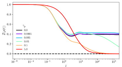
Figure 1: Time evolution of imbalance for a chain of $N=6$ sites, $V=2$ and $W=5$ with a bath consisting of $L_{j}=n_{j}$ measurements, where $\gamma_{p}$ spans many orders of magnitude. We see that within some window of $\gamma_{p}$ there is an enhancement in localization. All data points are averaged over $n_{d}=200$ disorder realisations and $n_{t}=500$ trajectories per realisation. [47]

In the second regime, with very large $\gamma_{p}$, we expect the effect of the measurements to dominate the behaviour of the system. This regime has been studied in detail recently [10, 12, 35, 45], under the guise of measurement induced criticality. For sufficiently strong measurement rate the system enters a disentangling phase where entanglement is suppressed, but the result is that excitations are evenly distributed throughout the system.

The third and final regime is for an intermediate coupling to the bath, where we see a pre-thermalization regime that has an enhancement in localization. Here, the interplay between unitary evolution and projective measurements results in a temporary stability with an enhanced localization signature, before an eventual thermalization. The temporary enhancement results from occupied sites being the most probable to be measured in the trajectory approach. For a large enough rate of measurement this preserves more information of the initial state for some time window, without completely dominating the dynamics. We now present the simulation results for this regime.

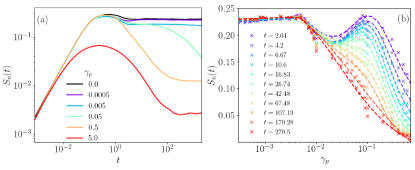
Figure 2: For a chain of $N=6$ sites, $V=2$ and $W=5$, we show (a) the logarithmic negativity against time after a partial transpose of half the system for various choices of $\gamma_{p}$, and (b) the logarithmic negativity against $\gamma_{p}$ for many different timeslices. In (a) we see that there is a reduction in entanglement as the influence of the bath becomes more dominant.

Imbalance.—The main result can be exemplified in Fig. 1, where the time evolution of the imbalance is shown for $L_{j}=n_{j}$ as the Lindblad operators. When $\gamma_{p}=0$ the imbalance reaches a steady state value that signals localization in the system. Note that in order to expose dominant features in the following numerical simulations we employ a moving average routine [48] to suppress noise and oscillatory behaviour.

For very small $\gamma_{p}$, such that the effective rate of measurement occurs a long time after the closed system reaches a steady state, we see that the pre-thermal regime is dictated by the coherent dynamics alone. After sufficient time has passed $\sim 1/\gamma_{p}$ the system begins to lose information and reduces to a $\mathcal{I}=0$ thermal state. For intermediate $\gamma_{p}$, where the rate of measurement occurs at a similar time to the closed system reaching a steady state, we see an enhancement in localization for a time window before an eventual thermalization. We thus call this a pre-thermalization regime with enhanced localization. For very large $\gamma_{p}$, we see information preserved for a longer time, but an eventual thermalization without an intermediate pre-thermalization regime.

Logarithmic Negativity.—In Fig. 2 (a), we simulate the evolution of entanglement via the logarithmic negativity $S_{n}(t)$. We see an initial linear growth in entanglement that overshoots and plateaus off when $\gamma_{p}=0$. This cutoff is dictated by the system size and we expect it to grow logarithmically as $N$ is increased [28]. For very small $\gamma_{p}$ we see very little deviation in the plateau, as expected from the analysis of imbalance in Fig. 1. For values of $\gamma_{p}$ where there is an enhancement of localization, we see a reduction in entanglement, evidenced by a plateau at a smaller value of $S_{n}(t)$. This is in line with the intuition that when more initial state information is retained there is less build up of correlations and therefore less entanglement between subsystems. For very large $\gamma_{p}$ the dynamics are entirely dominated by the disentangling nature of the environment.

In Fig. 2 (b), we show how $S_{n}(t)$ changes with increasing $\gamma_{p}$ for different choices of time. For small values of $\gamma_{p}$ we see very little deviation in $S_{n}(t)$, signalling that the bath does not influence dynamics at this timescale. At intermediate $\gamma_{p}$ there is a clear dip in $S_{n}(t)$ that corresponds to the regions in Fig. 1 for which we see an enhancement in localization. For larger $\gamma_{p}$ there is a sharp decrease in the entanglement between subsystems, dominated by the influence of the environment.

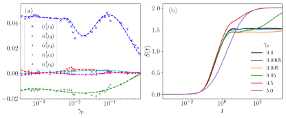
Figure 3: For a chain of $N=6$ sites, $V=2$ and $W=5$, we show (a) two-point correlations from the first site to all other sites across many values of $\gamma_{p}$ at time $t=10.6$s, and (b) the change in von Neumann entropy with time for various choices of $\gamma_{p}$. In (a), there is a signature of reduced entanglement in the nearest neighbour correlation between sites $1$ and $2$ for an intermediate region of $\gamma_{p}$ that is in agreement with (b).

Correlations.—In Fig. 3 (a), we show $2$-point correlations in the chain for varying coupling strength at time $t=10.6s$. Most enlightening is the nearest neighbour correlation. Initially this remains close to constant and is fit with a linear function. After reaching large enough $\gamma_{p}$ we see a reduction in its values, signalling less information transported along the chain at this time. The eventual rise in value signals a departure from the enhanced regime, before a second decay as the system enters the Zeno phase. The region of the dip is in exact correspondence with the dip seen in Fig. 2 (b) that determines the region of enhanced localization.

Finally, in Fig. 3 (b) we show how the von Neumann entropy changes with time for different choices of $\gamma_{p}$. Keeping in mind that this includes both quantum and classical correlations, we now see that for large $\gamma_{p}$ the value of $S(t)$ increases beyond the $\gamma_{p}=0$ case, even though $S_{n}(t)$ decreases. For very small $\gamma_{p}$, at the timescale shown, the system behaves much like the closed system as expected from previous figures. But in the intermediate regime there is an initial plateau with a lower entropy than for $\gamma_{p}=0$, before an eventual growth. This can be attributed to a reduction in quantum correlations due to the enhanced localization, followed by a growth in thermalization or classical correlations dictated by the environment.

From these simulations we can conclude that there exists a finite window where localization is (atleast temporarily) enhanced by the presence of the environment. For very small values of coupling there is little effect on the system. For very large coupling the environment dominates the behaviour and the system disentangles. Whilst this results in a slow down in the thermalization process, as evidenced by the imbalance and slow growth of entropy, it will always lead to thermalization in the system.

Lieb-Robinson bound and prethermal regime.—The results presented above can be supported by considering the speed at which information propagates along the chain [49, 50]. Here, we utilize the results in Ref. [49] to obtain a Lieb-Robinson bound for an open system influenced by measurements satisfying $L_{j}\equiv P_{j}=P_{j}^{2}$. The Lieb-Robinson bound can be expressed as an upper bound on the Lieb-Robinson commutator [51, 52, 49]

$$C_{B}(x,t)=\sup_{A_{x}}\frac{\left|\left|\left[A_{x},B(t)\right]\right|\right|}{\left|\left|A_{x}\right|\right|},$$ (3)

where $\left|\left|O\right|\right|$ is the operator norm of the operator $O$, $A_{x}$ is an operator acting on site $x$ and $B(t)=\mathbb{E}_{\xi}B_{\xi}(t)$ is an operator in the Heisenberg picture that may have support over many sites, disorder averaged over realisations $\xi$. To determine $B(t)$ we require the adjoint Lindblad master equation to given by $\mathcal{L}^{\dagger}B(t)=i\left[H,B(t)\right]-\gamma\mathcal{D}(B)$ where $\mathcal{D}(B(t))$ is the dissipator, the term in Eq. (2) containing the Lindblad operators.

Following the steps taken in [49], we find the following bound for an open system under the influence of measurements,

$$C_{B}(x,t)\leq e^{(-2\gamma_{p}p+4\left|\left|H\right|\right|)t}\sum_{j}^{N}e^{2\left|\left|H\right|\right|R_{x,j}t}C_{B}(j,0),$$ (4)

where we assume $\sum_{j}P_{j}B(t)\leq pB(t)$ and $R_{j,k}=\delta_{j,k+1}+\delta_{j+1,k}$. Assuming no particle loss in the system, we may choose our measurement operator to be the fermionic occupation number, i.e. $P_{j}=n_{j}$, so that $p\equiv\sum_{j}n_{j}$ the total number of fermions in the system. In our work we intialize the system at half-filling, so $p=N/2$, and this is fixed throughout the dynamics. We present a thorough analysis of the applicability of this bound in the limit of very small and very large measurement strength in the Supplemental Material [41], however, here we explore only the regime that induces an enhancement in the prethermal regime.

Given that $\left|\left|R\right|\right|=2$, if $\gamma_{p}>\frac{4\left|\left|H\right|\right|}{p}$ then the exponentially decreasing part of our bound is dominant. When $t<1/\gamma_{p}$ the open system dynamics remain negligible and dynamics will follow the closed chain. When $t\sim 1/\gamma_{p}$ the closed system bound [53] is no longer applicable and we must consider the dynamics induced within the constraint of the dominant part of our bound. This bound is negligible when either $|j-k|\geq tc_{\chi}$ for a constant $c_{\chi}>0$ or when $t\geq t_{\chi}=\log(\frac{C}{\chi})/\Gamma$, with $C=\sum_{j}C_{B}(j,0)$, $\Gamma=2\gamma_{p}p+8\left|\left|H\right|\right|$ and $\chi$ a constant. Here, $\Gamma$ is chosen to cancel any contribution from the exponentially growing part of the bound. Combining these two conditions, we have that the bound is non-negligible only when $\left|j-k\right|<c_{\chi}t_{\chi}$, which is a constant. This constant implies localization as correlations can only spread up to a finite number of sites. However, for very long times and small system sizes, the condition $|j-k|\geq tc_{\chi}$ implies that correlations may still spread across the entire system. In this case we expect an eventual thermalization that follows a pre-thermalization regime.

Interpreting enhancement from unification of measurements and disorders.—Note that the Lindblad master equation Eq. (2) with jump operator $L_{j}=n_{j}$ for the unconditional measurements also describes the effect of dephasing noise. Existing works reveal slow-down and heating effects of such noise [54, 55, 56, 57, 58], which will even destroy many-body localization [59, 60, 61, 62]. Therefore, the pre-thermal enhancement of localization observed in this work is rather surprising. In recent work [23], it is shown that projective measurements and disorders are unified in Keldysh field theory. Specifically, the corresponding Keldysh action of Eq. (2) is in a similar form as that of a disordered free-fermion gas [63, 64, 65], and in the long-time steady regime, a Drude-form conductivity is obtained. In addition to the similarity, the measurement case will introduce an extra decoherence effect due to the nature of open systems. This decoherence effect will turn the quantum system into a classical one, and then hides similar exotic effects as that produced by disorders in a quantum system, such as weak localization and many-body localization.

From the above discussion, one finds that the similarity with disorders can be further revealed when the decoherence effect is suppressed in the projective measurement case. A possible way to reduce the decoherence effect is to consider small values of measurement strength $\gamma$ and short-time dynamics of the monitored system. In this scenario, the decoherence is small at each time step and will not sufficiently accumulate in a short time period. Indeed, this is the regime at which we observed the enhancement of many-body localization shown in Figs. 1–3. In this regime, decoherence is suppressed and projective measurements will act like disorders in a quantum system, then the disorder strength $W$ is in turn effectively increased, and thus the enhancement of many-body localization appears.

Discussion.—In this work we have exposed a regime of enhanced localization due to the interplay of MBL and Zeno physics. When the MBL system is coupled to an external bath, the bath serves as a source of energy and particle exchange, driving the system towards thermalization. However, the Lieb-Robinson bound restricts the speed of information propagation in the system, effectively slowing down the dynamics of the MBL system as it interacts with the bath. Therefore, even though the bath promotes delocalization or thermalization, the process is slowed down by the constraints imposed by Eq. (4). The pre-thermal phase is characterized by the system exhibiting both localized and thermalized features, as the system resists full thermalization for a relatively long time. The details of the pre-thermal phase depends on factors such as the strength of coupling between the system and the bath, the degree of disorder, and the strength of the interactions in the system. The enhancement of the localization can be understood from a Keldysh nonlinear sigma model [23], if we take into account the restoration of coherence within the prethermal regime.

Further, we believe that this result may influence ongoing MBL simulations, for e.g. [3], where decoherence effects are ignored due to the dephasing time of qubits being slower than the experimental time. Finally, we envisage that our result will be directly observable on current quantum devices capable of simulating hybrid quantum circuit models, see for e.g. [10], that consist of both unitary dynamics and random measurements, by interlacing the MBL architecture with random measurements.

Supplemental Material: Enhanced localization in the prethermal regime of continuously measured many-body localized systems

In the supplemental material we provide further details to support the main text. In Sec. .1, we present the quantum trajectory approach employed here to find the time evolution of a quantum system under the influence of measurements. In Sec. .2 we present a corrected result from the V1 arXiv submission. Here we show that scalar transformations on the Lindblad operators should render the imbalance unchanged. Further, we present the imbalance data given in the main text, but without using the moving average smoothing routine. In Sec. .3, we give the mathematical steps required to derive the Lieb-Robinson bound used to support our numerical study. Finally, in Sec. .4, we provide a more detailed analysis of the applicability of the Lieb-Robinson bound, particularly in the cases of very small and very large measurement rate outside the regime of enhanced localization.

.1 Quantum trajectory approach for open system dynamics

Here we outline the quantum trajectory for open quantum systems, as implemented by the QuTiP numerical package [40]. In our work, we require many disorder realisations, so the outlined steps must be completed for each disorder realisation. Setting $\hbar=1$ throughout, first choose an initial state $\left|\psi(0)\right\rangle$ at time $t=0$. Then, evolve in time with the non-Hermitian Hamiltonian

$$H_{\mathrm{nh}}=H-\frac{i}{2}\sum_{j}L^{\dagger}_{j}L$$ (S1)

via $i\frac{\text{d}}{\text{dt}}\left|\psi(t)\right\rangle=H_{\text{nh}}\left|\psi(t)\right\rangle$. This does not preserve the norm of the state $\left|\psi(t)\right\rangle$ as the Hamiltonian is non-Hermitian. When the norm is less than a randomly generated number $p_{1}$

$$\left\langle\psi(t)\right|\left.\!\psi(t)\right\rangle<p_{1},$$ (S2)

perform a quantum jump. The choice of jump operator is also implemented randomly, choose a second randomly generated number $p_{2}$. For each operator calculate the probability for a jump to occur by

$$\mathrm{Pr}_{j}(t)=\frac{\left\langle\psi(t)\right|L^{\dagger}_{j}L_{j}\left|\psi(t)\right\rangle}{\sum_{k}\left\langle\psi(t)\right|L^{\dagger}_{k}L_{k}\left|\psi(t)\right\rangle}.$$ (S3)

The choice of operator is given by the smallest $n$ that satisfies

$$\sum_{n}\mathrm{Pr}_{n}(t)\geq p_{2}.$$ (S4)

Then, perform a quantum jump and renormalise the state

$$\left|\psi(t)\right\rangle\to\frac{L_{n}\left|\psi(t)\right\rangle}{|L_{n}\left|\psi(t)\right\rangle|}.$$ (S5)

Finally, continue to coherently evolve the system until the norm of the state once again a new randomly generated number and perform a quantum jump. This procedure is repeated until the full time evolution is complete.

This process provides a single trajectory and demonstrates the random nature of the environment on the system. Note that, the exact density matrix is recovered in the infinite trajectory limit $\rho(t)=\lim_{n_{t}\to\infty}\frac{1}{n_{t}}\sum_{j}^{n_{t}}\left|\psi^{(j)}(t)\right\rangle\!\!\left\langle\psi^{(j)}(t)\right|$, likewise we may recover observables of the system exactly in the same limit $\text{tr}\left[\mathcal{O}\rho(t)\right]=\lim_{n_{t}\to\infty}\frac{1}{n_{t}}\sum_{j=1}^{n_{t}}\left\langle\psi^{(j)}(t)\right|\mathcal{O}\left|\psi^{(j)}(t)\right\rangle$. In this work we simulate sufficiently many trajectories $n_{t}=500$ to recover accurate statistics of the dynamics.

.2 Imbalance for non-projective choice of Lindblad operator

In V1 we showed that by choosing the Lindblad operator to be $L_{j}=n_{j}-\frac{1}{2}$ there is no enhancement in localization. However, the Lindblad master equation is invariant under the scaling transformation $L_{j}\to L_{j}+\alpha_{j}\mathbb{I}$, with $\alpha_{j}$ an arbitrary constant. We therefore expect the results for $L_{j}=n_{j}-\frac{1}{2}$ (with measurement rate $\gamma_{n}$) to be consistent with $L_{j}=n_{j}$ (with measurement rate $\gamma_{p}$). In order to verify this we increased the number of trajectories sampled from $500$ in V1 to $1000$ in V2. Now, we see that the two choices of Lindblad operator produce consistent results.

In Fig. S1 we demonstrate this for the choice of $\gamma_{p(n)}=0.05$. As a sanity check, we have also increased the number of trajectories for another choice of $\gamma_{p}$ to confirm the accuracy of the results presented in the main text. The cyan curve shows the result for $\gamma_{p}=0.005$ and $n_{t}=1000$, with $L_{j}=n_{j}$. This produces the same result as that given in the main text, highlighting the applicability of $n_{t}$ used to demonstrate the result in the main text. The purple curve shows the result for $\gamma_{p}=0.05$ and $n_{t}=500$, with $L_{j}=n_{j}$. This is the result given in the main text and is used for comparison with the orange dashed curve, where now $\gamma_{n}=0.05$ and $n_{t}=1000$ with $L_{j}=n_{j}-\frac{1}{2}$. We see that with more trajectories the results lie very close to each other and become almost indistinguishable, which is in agreement with the invariance of the Lindblad master equation after a scaling transformation. Thus, we see an enhancement in localization for both choices of Lindblad operator.

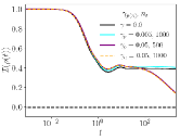
Figure S1: Imbalance for a chain of $N=6$ sites with an increased number of trajectories, given in the legend. The corrected data is given by the orange dashed line, where we see that the behaviour for both choices of Lindblad operator coincide providing enough trajectories are taken.

For transparency, in Fig. S2 we show the data presented in Fig. 1 of the main text without using the moving average smoothing routine [48]. While this routine highlights dominant features, it may also hide less dominant features within the data. It can be seen from this figure that the purpose of using the routine is only to suppress noise fluctuations and to highlight the enhanced localization that is discussed. There remains a clear separation between the curves for no disorder (black) and small disorder (purple) from those with intermediate values of disorder (blue and green), with high disorder curves (orange and red) not showing a prethermal regime.

.3 Lieb-Robinson bound for an open system under the influence of repeated measurements

In this section we present full details for the derivation of a Lieb-Robinson bound for an open system, where the Lindblad operators sayisfy $L_{j}\equiv P_{j}=P_{j}^{2}$. It is based on a similar calculation found in [49]. The following method is general, but makes a number of assumptions. First, assume a time-independent Hamiltonian with nearest-neighbour interactions at most, that is $H=\sum_{j}h_{j}$ where $h_{j}$ acts on sites $j$ and $j+1$. The Hamiltonian contains static disorder, so all observable quantities are calculated as an ensemble average over each disorder realisation $\xi$. For example, the density matrix is given by $\rho(t)=\mathbb{E}_{\xi}\rho(\xi,t)$. Assuming Markovian evolution, we model the dynamics by the Lindblad master equation

$$\partial_{t}\rho(t) =-i\left[H,\rho(t)\right]-\gamma\sum_{j}\left[\left[\rho(t),P_{j}\right],P_{j}\right]$$ (S6)

$$=\mathcal{L}\rho(t)$$

where $P_{j}$ is a measurement operator and $1/\gamma$ is the effective rate of measurement. Note that setting $\gamma\rightarrow\gamma/2$ recovers the standard form of the Lindblad master equation given in the main text.

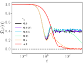
Figure S2: Imbalance for a chain of $N=6$ sites without smoothing using the moving average routine. Even without smoothing, there is clear distinction between the three regimes of interest within the timescales analysed: MBL dominant for small $\gamma_{p}$, enhanced localization for intermediate $\gamma_{p}$, and measurement dominant for large $\gamma_{p}$.

A Lieb-Robinson bound can be expressed as an upper bound on the Lieb-Robinson commutator

$$C_{B}(x,t)=\sup_{A_{x}}\frac{\left|\left|\left[A_{x},B(t)\right]\right|\right|}{\left|\left|A_{x}\right|\right|},$$ (S7)

where $\left|\left|O\right|\right|$ is the operator norm of the operator $O$, $A_{x}$ is an operator acting on site $x$ and $B(t)=\mathbb{E}_{\xi}B_{\xi}(t)$ is an operator in the Heisenberg picture that may have support over many sites. To determine $B(t)$ we require the adjoint Lindblad master equation to find the time evolution of operators. It is given by

$$\mathcal{L}^{\dagger}B(t)=i\left[H,B(t)\right]-\gamma\mathcal{D}(B)$$ (S8)

where the dissipator is $D(B(t))=\sum_{j}D_{j}(B(t))=\sum_{j}\left[P_{j},\left[P_{j},B(t)\right]\right]$. To approximate $\left|\left|\left[A_{x},B(t)\right]\right|\right|$ we take a Taylor expansion of $B(\tilde{t})$ with $\tilde{t}=t+\epsilon$. Up to order $\epsilon^{2}$, we have

$$\left|\left|\left[A_{x},B(\tilde{t})\right]\right|\right|=||\left[A_{x},B(t)\right]+\epsilon\left[A_{x},\partial_{t}B(t)\right]+\frac{\epsilon^{2}}{2}\left[A_{x},\partial_{t}^{2}B(t)\right]+\mathcal{O}(\epsilon^{3})||.$$ (S9)

Now, we expand each term individually. First, the $\mathcal{O}(\epsilon)$ term is given simply by the adjoint master equation, i.e.

$$\epsilon\left[A_{x},\partial_{t}B(t)\right] =\epsilon\left[A_{x},i\left[H,B\right]-\gamma\mathcal{D}\right]$$ (S10)

$$=i\epsilon\left[A_{x},\left[H,B\right]\right]-\epsilon\gamma\left[A_{x},\mathcal{D}\right].$$ (S11)

The $\mathcal{O}(\epsilon^{2})$ term requires taking the time derivative of the time-dependent terms of the adjoint master equation, as follows:

$$\frac{\epsilon^{2}}{2}\left[A_{x},\partial_{t}^{2}B(t)\right] =\frac{\epsilon^{2}}{2}\left[A_{x},\partial_{t}(i\left[H,B\right]-\gamma\mathcal{D})\right]$$ (S12)

$$=\frac{i\epsilon^{2}}{2}\left[A_{x},\left[H,\partial_{t}B\right]\right]-\frac{\epsilon^{2}\gamma}{2}\left[A_{x},\partial_{t}\mathcal{D}\right]$$ (S13)

$$=\frac{-\epsilon^{2}}{2}\left[A_{x},\left[H,\left[H,B\right]\right]\right]-\frac{i\epsilon^{2}\gamma}{2}\left[A_{x},\left[H,\mathcal{D}\right]\right]-\frac{\epsilon^{2}\gamma}{2}\left[A_{x},\partial_{t}\mathcal{D}\right].$$ (S14)

Assuming that $\sum_{j}P_{j}B\leq pB$, the final term is given by

$$[A_{x},\partial_{t}\mathcal{D}]=2ip\left[A_{x},\left[H,B\right]\right] -2\gamma p\left[A_{x},\mathcal{D}\right]-2[A_{x},\sum_{j}P_{j}\partial_{t}B(t)P_{j}].$$ (S15)

By only keeping $\mathcal{O}(\epsilon^{2})$ terms that also appear at $\mathcal{O}(\epsilon)$ and using the triangle inequality results in the following bound:

$$\left|\left|\left[A_{x},B(\tilde{t})\right]\right|\right|\leq (1-\epsilon\gamma p)\left|\left|\left[A_{x},B(t)+i\epsilon\left[H,B(t)\right]\right]\right|\right|+\epsilon\gamma\left|\left|\left[A_{x},pB+(\epsilon\gamma p-1)\mathcal{D}\right]\right|\right|+\mathcal{O}(\epsilon^{2}).$$ (S16)

We now bound each term individually. Using the unitary equivalence of the operator norm and by repeated Taylor expansions, the first term is bounded by

$$\left|\left|\left[A_{x},B(t)+i\epsilon\left[H,B(t)\right]\right]\right|\right|\leq\left|\left|\left[A_{x},B(t)\right]\right|\right|+\epsilon\left|\left|\left[\left[H,A_{x}\right],B(t)\right]\right|\right|.$$ (S17)

The second term is

$$\left|\left|\left[A_{x},pB+(\epsilon\gamma p-1)\mathcal{D}\right]\right|\right|\leq p\left|\left|\left[A_{x},B(t)\right]\right|\right|+(\epsilon\gamma p-1)\left|\left|\left[A_{x},\mathcal{D}\right]\right|\right|.$$ (S18)

Again, keeping only terms that already appear at $\mathcal{O}(\epsilon)$ the bound is reduced to

$$\left|\left|\left[A_{x},B(\tilde{t})\right]\right|\right|\leq (1-2\epsilon\gamma p+2\epsilon^{2}\gamma^{2}p^{2})\left|\left|\left[A_{x},B(t)\right]\right|\right|+\epsilon(1-\epsilon\gamma p)\left|\left|\left[\left[H,A_{x}\right],B(t)\right]\right|\right|+\mathcal{O}(\epsilon^{2}).$$ (S19)

It follows that the time derivative of the Lieb-Robinson correlator is bound by

$$\partial_{t}C_{B}(x,t)\leq-2\gamma pC_{B}(x,t)+\sup_{A_{x}}\frac{\left|\left|\left[\left[H,A_{x}\right],B(t)\right]\right|\right|}{\left|\left|A_{x}\right|\right|}.$$ (S20)

In order to solve this, we must expand the double commutator on the right. First note that, for our fermionic system with nearest-neighbour interactions, $\left[H,A_{x}\right]=2\left|\left|H\right|\right|\left|\left|A_{x}\right|\right|V$ with $V=u_{x-1}n_{x-1}n_{x}+u_{x}n_{x}n_{x-1}$ and $|u_{y}|\leq\left|\left|V\right|\right|\leq 1$. The operator $V$ will contribute both diagonal and off-diagonal components and can be bound by $V\leq 2\mathbb{I}+R$, where $R_{j,k}=\delta_{j,k+1}+\delta_{j+1,k}$. We may also express components $C_{B}(x,t)$ as a vector $C_{B}(t)=[C_{B}(1,t),\dots,C_{B}(N,t)]$, resulting in the bound

$$\partial_{t}C_{B}(t)\leq((-2\gamma p+4\left|\left|H\right|\right|)\mathbb{I}+2\left|\left|H\right|\right|R)C_{B}(t),$$ (S21)

where the inequality is evaluated component-wise. This bound emits the final solution

$$C_{B}(x,t)\leq e^{(-2\gamma p+4\left|\left|H\right|\right|)t}\sum_{j}^{N}\left(e^{2\left|\left|H\right|\right|Rt}\right)_{x,j}C_{B}(j,0).$$ (S22)

.4 Applicability of generalized Lieb-Robinson bound in the limit of very small and very large measurement rate

It is important for this analysis to reference other bounds related to this system. First, for a closed MBL system with interactions and disorder there exists a Lieb-Robinson bound that results in a logarithmic light cone [53, 66]. Second, for general open quantum systems with Markovian dynamics the Lieb-Robinson bound has been shown to have a ballistic light cone for Liouvillians that are the sum of local parts [67]. In both cases, outside of the light cone correlations decay exponentially fast. The main difference between Eq. (S22) and the general bound for open quantum systems is that the general bound will always allow for ballistic spreading of correlations, causing the system to thermalize. On the other hand, if the exponentially decaying part of Eq. (S22) is dominant then it is possible for information to be retained for some finite time when the system undergoes time evolution. In the limit that $\gamma_{p}\to 0$, Eq. (S22) returns to a bound where correlations spread ballistically. However, it should be noted that Eq. (S22) does not consider any microscopic details of the Hamiltonian, so there may exist a tighter bound when taking these details into account.

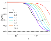
Figure S3: Imbalance for a chain of $N=6$ sites with $\gamma_{p}$ chosen to be large enough such that bath effects are dominant. For increasing $\gamma_{p}$ the eventual thermalization process is slowed down and the system retains initial information for increasing time.

Returning to the bound derived in Eq. (S22), and keeping in mind that $\left|\left|R\right|\right|=2$, if $\gamma_{p}<\frac{4\left|\left|H\right|\right|}{p}$ then Eq. (S22) is exponentially growing and the bounds discussed previously will provide a more appropriate restriction on the spread of correlations, that depends on how much time has passed in the evolution. Providing $t<1/\gamma_{p}$, the open system dynamics are negligible and the system will follow the closed system dynamics with correlations spreading logarithmically with time [53]. After sufficiently long time $t\sim 1/\gamma_{p}$, the open system dynamics become relevant and the general open system bound is applicable resulting in ballistic spreading of correlations. Thus, for very small $\gamma_{p}$ we see initial localization properties akin to the closed system, followed by an eventual thermalization. Thus, in the limit $\gamma_{p}<\frac{4\left|\left|H\right|\right|}{p}$ we expect a prethermal regime that is dictated by the coherent dynamics alone.

Conversely, if $\gamma_{p}\gg\frac{4\left|\left|H\right|\right|}{p}$, so that the timescale for unitary closed system dynamics is longer than the effective rate of measurement, the system will only follow the closed system dynamics for a very short time. Now, similarly to the discussion in the main text for the intermediate regime, the bound is negligible when either $|j-k|\geq tc_{\chi}$ for a constant $c_{\chi}>0$ or when $t\geq t_{\chi}=\log(\frac{C}{\chi})/\Gamma$, with $C=\sum_{j}C_{B}(j,0)$, $\Gamma=2\gamma_{p}p+8\left|\left|H\right|\right|$ and $\chi$ a constant. Here, $\Gamma$ is chosen to cancel any contribution from the exponentially growing part of the bound. Combining these two conditions, we have that the bound is non-negligible only when $\left|j-k\right|<c_{\chi}t_{\chi}$, which is a constant. This constant implies localization as correlations can only spread up to a finite number of sites. Thus we expect to see localization properties up to a time given by $|j-k|\geq tc_{\chi}$, after which, due to the finite size of the system, we expect thermalization. This is known as the Zeno regime where frequent repeated measurements retain information in the system.

To exemplify the applicability of this bound, in Fig. S3 we consider the case when $\gamma_{p}$ is very large so that dynamics are entirely dominated by the bound for both small and large timescales. It is clear that as the value of $\gamma_{p}$ increases the amount of time that information of the initial state remains also extends, before an eventual decay to a thermalized state. This is due to the repeated measurements constantly resetting the initially occupied states back to certain occupation. This can also be explained by analysing the bound. From the conditions above we find that $t_{\chi}\sim 1/\gamma_{p}$. Thus, for larger $\gamma_{p}$, due to the bound $\left|j-k\right|<c_{\chi}t_{\chi}$, the spread of correlations is pinned tighter than for smaller $\gamma_{p}$.

References

- Preskill [2018] J. Preskill, Quantum Computing in the NISQ era and beyond, Quantum 2, 79 (2018).
- Smith et al. [2016] J. Smith, A. Lee, P. Richerme, B. Neyenhuis, P. W. Hess, P. Hauke, M. Heyl, D. A. Huse, and C. Monroe, Many-body localization in a quantum simulator with programmable random disorder, Nature Phys. 12, 907 (2016).
- Xu et al. [2018] K. Xu, J.-J. Chen, Y. Zeng, Y.-R. Zhang, C. Song, W. Liu, Q. Guo, P. Zhang, D. Xu, H. Deng, K. Huang, H. Wang, X. Zhu, D. Zheng, and H. Fan, Emulating many-body localization with a superconducting quantum processor, Phys. Rev. Lett. 120, 050507 (2018).
- Guo and Li [2018] X. Guo and X. Li, Detecting many-body-localization lengths with cold atoms, Phys. Rev. A 97, 033622 (2018).
- Zhu et al. [2021] D. Zhu, S. Johri, N. Nguyen, C. H. Alderete, K. Landsman, N. Linke, C. Monroe, and A. Matsuura, Probing many-body localization on a noisy quantum computer, Phys. Rev. A 103, 032606 (2021).
- Žnidarič [2010] M. Žnidarič, Dephasing-induced diffusive transport in the anisotropic heisenberg model, New J. Phys. 12, 043001 (2010).
- Nandkishore et al. [2014] R. Nandkishore, S. Gopalakrishnan, and D. A. Huse, Spectral features of a many-body-localized system weakly coupled to a bath, Phys. Rev. B 90, 064203 (2014).
- Levi et al. [2016] E. Levi, M. Heyl, I. Lesanovsky, and J. P. Garrahan, Robustness of many-body localization in the presence of dissipation, Phys. Rev. Lett. 116, 237203 (2016).
- Nandkishore [2015] R. Nandkishore, Many-body localization proximity effect, Phys. Rev. B 92, 245141 (2015).
- Li et al. [2018] Y. Li, X. Chen, and M. P. Fisher, Quantum zeno effect and the many-body entanglement transition, Phys. Rev. B 98, 205136 (2018).
- Chan et al. [2019] A. Chan, R. M. Nandkishore, M. Pretko, and G. Smith, Unitary-projective entanglement dynamics, Phys. Rev. B 99, 224307 (2019).
- Skinner et al. [2019] B. Skinner, J. Ruhman, and A. Nahum, Measurement-induced phase transitions in the dynamics of entanglement, Phys. Rev. X 9, 031009 (2019).
- AI and Collaborators [2023] G. Q. AI and Collaborators, Quantum information phases in space-time: measurement-induced entanglement and teleportation on a noisy quantum processor (2023), arXiv:2303.04792 .
- Nahum et al. [2017] A. Nahum, J. Ruhman, S. Vijay, and J. Haah, Quantum entanglement growth under random unitary dynamics, Phys. Rev. X 7, 031016 (2017).
- Khemani et al. [2018] V. Khemani, A. Vishwanath, and D. A. Huse, Operator spreading and the emergence of dissipative hydrodynamics under unitary evolution with conservation laws, Phys. Rev. X 8, 031057 (2018).
- Sünderhauf et al. [2018] C. Sünderhauf, D. Pérez-García, D. A. Huse, N. Schuch, and J. I. Cirac, Localization with random time-periodic quantum circuits, Phys. Rev. B 98, 134204 (2018).
- Jian et al. [2020] C.-M. Jian, Y.-Z. You, R. Vasseur, and A. W. W. Ludwig, Measurement-induced criticality in random quantum circuits, Phys. Rev. B 101, 104302 (2020).
- Misra and Sudarshan [1977] B. Misra and E. G. Sudarshan, The zeno’s paradox in quantum theory, J. Math. Phys. 18, 756 (1977).
- Huse et al. [2015] D. A. Huse, R. Nandkishore, F. Pietracaprina, V. Ros, and A. Scardicchio, Localized systems coupled to small baths: From anderson to zeno, Phys. Rev. B 92, 014203 (2015).
- Maimbourg et al. [2021] T. Maimbourg, D. M. Basko, M. Holzmann, and A. Rosso, Bath-induced zeno localization in driven many-body quantum systems, Phys. Rev. Lett. 126, 120603 (2021).
- Ippoliti et al. [2021] M. Ippoliti, M. J. Gullans, S. Gopalakrishnan, D. A. Huse, and V. Khemani, Entanglement phase transitions in measurement-only dynamics, Phys. Rev. X 11, 011030 (2021).
- Halimeh et al. [2022] J. C. Halimeh, L. Homeier, H. Zhao, A. Bohrdt, F. Grusdt, P. Hauke, and J. Knolle, Enhancing disorder-free localization through dynamically emergent local symmetries, PRX Quantum 3, 020345 (2022).
- Yang et al. [2023] Q. Yang, Y. Zuo, and D. E. Liu, Keldysh nonlinear sigma model for a free-fermion gas under continuous measurements (2023), arXiv:2207.03376 .
- Oganesyan and Huse [2007] V. Oganesyan and D. A. Huse, Localization of interacting fermions at high temperature, Phys. Rev. B 75, 155111 (2007).
- Pal and Huse [2010] A. Pal and D. A. Huse, Many-body localization phase transition, Phys. Rev. B 82, 174411 (2010).
- Serbyn et al. [2013] M. Serbyn, Z. Papić, and D. A. Abanin, Universal slow growth of entanglement in interacting strongly disordered systems, Phys. Rev. Lett. 110, 260601 (2013).
- Alet and Laflorencie [2018] F. Alet and N. Laflorencie, Many-body localization: An introduction and selected topics, Comptes Rendus Physique 19, 498 (2018).
- Abanin et al. [2019] D. A. Abanin, E. Altman, I. Bloch, and M. Serbyn, Colloquium: Many-body localization, thermalization, and entanglement, Rev. Mod. Phys. 91, 021001 (2019).
- Sarkar et al. [2014] S. Sarkar, S. Langer, J. Schachenmayer, and A. J. Daley, Light scattering and dissipative dynamics of many fermionic atoms in an optical lattice, Phys. Rev. A 90, 023618 (2014).
- Schreiber et al. [2015] M. Schreiber, S. S. Hodgman, P. Bordia, H. P. Lüschen, M. H. Fischer, R. Vosk, E. Altman, U. Schneider, and I. Bloch, Observation of many-body localization of interacting fermions in a quasirandom optical lattice, Science 349, 842 (2015).
- Luitz et al. [2015] D. J. Luitz, N. Laflorencie, and F. Alet, Many-body localization edge in the random-field heisenberg chain, Phys. Rev. B 91, 081103 (2015).
- Fischer et al. [2016] M. H. Fischer, M. Maksymenko, and E. Altman, Dynamics of a many-body-localized system coupled to a bath, Phys. Rev. Lett. 116, 160401 (2016).
- Everest et al. [2017] B. Everest, I. Lesanovsky, J. P. Garrahan, and E. Levi, Role of interactions in a dissipative many-body localized system, Phys. Rev. B 95, 024310 (2017).
- Hamazaki et al. [2019] R. Hamazaki, K. Kawabata, and M. Ueda, Non-hermitian many-body localization, Phys. Rev. Lett. 123, 090603 (2019).
- Fuji and Ashida [2020] Y. Fuji and Y. Ashida, Measurement-induced quantum criticality under continuous monitoring, Phys. Rev. B 102, 054302 (2020).
- Breuer et al. [2002] H.-P. Breuer, F. Petruccione, et al., The theory of open quantum systems (Oxford University Press, 2002).
- Dalibard et al. [1992] J. Dalibard, Y. Castin, and K. Mølmer, Wave-function approach to dissipative processes in quantum optics, Phys. Rev. Lett. 68, 580 (1992).
- Pichler et al. [2010] H. Pichler, A. J. Daley, and P. Zoller, Nonequilibrium dynamics of bosonic atoms in optical lattices: Decoherence of many-body states due to spontaneous emission, Phys. Rev. A 82, 063605 (2010).
- Alberton et al. [2021] O. Alberton, M. Buchhold, and S. Diehl, Entanglement transition in a monitored free-fermion chain: From extended criticality to area law, Phys. Rev. Lett. 126, 170602 (2021).
- Johansson et al. [2012] J. Johansson, P. Nation, and F. Nori, Qutip: An open-source python framework for the dynamics of open quantum systems, Comput. Phys. Commun. 183, 1760 (2012).
- [41] See supplemental material for more details.
- Vidal and Werner [2002] G. Vidal and R. F. Werner, Computable measure of entanglement, Phys. Rev. A 65, 032314 (2002).
- Plenio [2005] M. B. Plenio, Logarithmic negativity: A full entanglement monotone that is not convex, Phys. Rev. Lett. 95, 090503 (2005).
- Calabrese et al. [2012] P. Calabrese, J. Cardy, and E. Tonni, Entanglement negativity in quantum field theory, Phys. Rev. Lett. 109, 130502 (2012).
- Sang et al. [2021] S. Sang, Y. Li, T. Zhou, X. Chen, T. H. Hsieh, and M. P. Fisher, Entanglement negativity at measurement-induced criticality, PRX Quantum 2, 030313 (2021).
- Shapourian and Ryu [2018] H. Shapourian and S. Ryu, Entanglement negativity of fermions: Monotonicity, separability criterion, and classification of few-mode states, Phys. Rev. A 99 (2018).
- [47] Note, that this figure has been corrected from arxiv submission v1 to v2, the correction is outlined in the supplemental material.
- Hyndman [2011] R. J. Hyndman, International Encyclopedia of Statistical Science, edited by M. Lovric (Springer Berlin Heidelberg, 2011) pp. 866–869.
- Burrell et al. [2008] C. Burrell, J. Eisert, and T. Osborne, Information propagation through quantum chains with fluctuating disorder, Phys. Rev. A 80 (2008).
- Vu and Das Sarma [2023] D. Vu and S. Das Sarma, Dissipative prethermal discrete time crystal, Phys. Rev. Lett. 130, 130401 (2023).
- Lieb and Robinson [1972] E. H. Lieb and D. W. Robinson, The finite group velocity of quantum spin systems, Commun. Math. Phys. 28, 251 (1972).
- Burrell and Osborne [2007] C. K. Burrell and T. J. Osborne, Bounds on the speed of information propagation in disordered quantum spin chains, Phys. Rev. Lett. 99, 167201 (2007).
- Kim et al. [2014] I. H. Kim, A. Chandran, and D. A. Abanin, Local integrals of motion and the logarithmic lightcone in many-body localized systems (2014), arXiv:1412.3073 .
- Žnidarič [2010a] M. Žnidarič, Exact solution for a diffusive nonequilibrium steady state of an open quantum chain, J. Stat. Mech. 2010, L05002 (2010a).
- Žnidarič [2010b] M. Žnidarič, Dephasing-induced diffusive transport in the anisotropic heisenberg model, New J. Phys. 12, 043001 (2010b).
- Sieberer et al. [2016] L. M. Sieberer, M. Buchhold, and S. Diehl, Keldysh field theory for driven open quantum systems, Rep. Prog. Phys. 79, 096001 (2016).
- Jin et al. [2022] T. Jin, J. a. S. Ferreira, M. Filippone, and T. Giamarchi, Exact description of quantum stochastic models as quantum resistors, Phys. Rev. Research 4, 013109 (2022).
- Turkeshi and Schiró [2021] X. Turkeshi and M. Schiró, Diffusion and thermalization in a boundary-driven dephasing model, Phys. Rev. B 104, 144301 (2021).
- Medvedyeva et al. [2016] M. V. Medvedyeva, T. c. v. Prosen, and M. Žnidarič, Influence of dephasing on many-body localization, Phys. Rev. B 93, 094205 (2016).
- Wu and Eckardt [2019] L.-N. Wu and A. Eckardt, Bath-induced decay of stark many-body localization, Phys. Rev. Lett. 123, 030602 (2019).
- Lüschen et al. [2017] H. P. Lüschen, P. Bordia, S. S. Hodgman, M. Schreiber, S. Sarkar, A. J. Daley, M. H. Fischer, E. Altman, I. Bloch, and U. Schneider, Signatures of many-body localization in a controlled open quantum system, Phys. Rev. X 7, 011034 (2017).
- Yamamoto and Hamazaki [2023] K. Yamamoto and R. Hamazaki, Localization properties in disordered quantum many-body dynamics under continuous measurement, Phys. Rev. B 107, L220201 (2023).
- Horbach and Schön [1993] M. L. Horbach and G. Schön, Dynamic nonlinear -model of electron localization, Annalen der Physik 505, 51 (1993).
- Finkel’Stein [1984] A. Finkel’Stein, Weak localization and coulomb interaction in disordered systems, Zeitschrift für Physik B Condensed Matter 56, 189 (1984).
- Kamenev [2011] A. Kamenev, Field theory of non-equilibrium systems (Cambridge University Press, 2011).
- Deng et al. [2017] D.-L. Deng, X. Li, J. H. Pixley, Y.-L. Wu, and S. Das Sarma, Logarithmic entanglement lightcone in many-body localized systems, Phys. Rev. B 95, 024202 (2017).
- Barthel and Kliesch [2012] T. Barthel and M. Kliesch, Quasilocality and efficient simulation of markovian quantum dynamics, Phys. Rev. Lett. 108, 230504 (2012).