As if Time Had Stopped – Checking Memory Dumps for Quasi-Instantaneous Consistency

Abstract

Memory dumps that are acquired while the system is running often contain inconsistencies like page smearing which hamper the analysis. One possibility to avoid inconsistencies is to pause the system during the acquisition and take an instantaneous memory dump. While this is possible for virtual machines, most systems cannot be frozen and thus the ideal dump can only be quasi-instantaneous, i.e., consistent despite the system running. In this article, we introduce a method allowing us to measure quasi-instantaneous consistency and show both, theoretically, and practically, that our method is valid but that in reality, dumps can be but usually are not quasi-instantaneously consistent. For the assessment, we run a pivot program enabling the evaluation of quasi-instantaneous consistency for its heap and allowing us to pinpoint where exactly inconsistencies occurred.

1 Introduction

The acquisition and analysis of main memory are common tasks for forensic investigators, e.g., to find encryption keys for storage or analyze malware that only runs in memory. A common acquisition procedure is to perform live memory acquisition, i.e., to utilize the software on the system under investigation to access and dump memory. However, as the system is running and memory contents are continuously updated by concurrent processes, the quality of such snapshots is (at best) unclear. A symptom of bad memory snapshots, that is commonly observed, is page smearing which is defined as “an inconsistency that occurs in memory captures when the acquired page tables reference physical pages whose contents changed during the acquisition process” (Case and Richard III, 2017). It is well-known that established tools like Volatility have difficulties parsing low-quality memory snapshots, resulting in cases where snapshots cannot be analyzed at all. But what, actually, is a “good” memory snapshot?

In practice, it is commonly accepted that freezing a system, i.e., stopping concurrent system activity before taking a memory snapshot, produces the highest quality. Such snapshots are often referred to as instantaneous snapshots. Methods to create instantaneous snapshots either have strong assumptions, e.g., assume that the analyzed system runs as a virtual machine (Martignoni et al., 2010; Yu et al., 2012; Kiperberg et al., 2019), or are cumbersome to execute, like cold boot attacks (Halderman et al., 2009; Bauer et al., 2016). Therefore, in many practical situations memory acquisition is necessarily performed live and the resulting snapshots are not instantaneous. But in what sense can non-instantaneous snapshots be compared regarding quality?

It has been observed (Pagani et al., 2019; Ottmann et al., 2022) that certain snapshots acquired live cannot be distinguished from instantaneous snapshots. Such snapshots are called time-consistent (Pagani et al., 2019) or quasi-instantaneous (Ottmann et al., 2022). By definition quasi-instantaneous snapshots avoid the many hassles associated with live memory acquisition, but unless the memory acquisition method itself provides consistency guarantees, it was not known how memory snapshots can be tested for quasi-instantaneous consistency. Clearly, such methods must rely on some form of consistency indicators within the image. How these may look like to precisely determine the consistency of a snapshot was so far unclear. In this article, we describe a method to measure quasi-instantaneous consistency of memory snapshots based on well-defined consistency indicators.

1.1 Related work

After multiple works about the quality of memory dumps (Inoue et al., 2011; Lempereur et al., 2012; Campbell, 2013), three formal criteria for the assessment of a memory dump’s quality were defined by Vömel and Freiling (2012): correctness, atomicity, and integrity. Correctness is fulfilled if the contents of the memory dump are an exact copy of the memory contents at the time of their acquisition. Atomicity addresses the causal consistency of the memory dump. It depends on the cause-effect relationships between memory accesses by different processes. The last criterion, integrity, is assessed in relation to a point in time shortly before the memory acquisition is started. Memory contents that change after this point in time and before they were copied by the memory acquisition program lower the degree of integrity of the memory dump. Two applications of the criteria for practical evaluations of memory acquisition methods followed: one with a white-box testing method (Vömel and Stüttgen, 2013), and one with a black-box testing method (Gruhn and Freiling, 2016).

In contrast to abstract measures such as atomicity, Pagani et al. (2019) took a content-based approach to assess the consistency of a memory dump. A memory dump is time-consistent if there “exists a hypothetical atomic acquisition process that could have returned the same result”. One method they applied in their evaluation to assess the consistency of a memory dump is the number of virtual memory areas (VMAs) that are attributed to a task by different sources. If the numbers differ an inconsistency in a memory dump has been spotted.

Based on the idea of time consistency, Ottmann et al. (2022) introduced two formal criteria, instantaneous consistency, and quasi-instantaneous consistency. While the former criterion portrays the ideal case for memory acquisition, pausing the system’s execution and copying all memory contents at the same time, the latter can be fulfilled even if the system cannot be paused. It requires that the contents of the memory dump could have also been acquired with a hypothetical instantaneous snapshot. Or in other words, there was a time at which the dump’s contents were coexistent in memory. Therefore, a memory dump that fulfills the latter criterion is as consistent as an instantaneous snapshot. So while quasi-instantaneous consistency is as good as instantaneous consistency, Ottmann et al. (2022) fail to give a method to check or observe it. Such a method would allow testing snapshots of benchmark acquisition methods to gain trust in data and methods.

1.2 Contributions

In this paper, we devise a method with which (under certain assumptions) it is possible to find out whether a portion of a snapshot is quasi-instantaneously consistent. Assumptions are the existence of consistency indicators in memory. These represent information on the last event that happened in a particular memory region and that potentially changed the content of that region. This extends the content-based approach of Pagani et al. (2019). Given such indicators, we show how it is possible to test whether a snapshot is quasi-instantaneously consistent. Furthermore, if a memory dump is not quasi-instantaneously consistent, we can use the output of the method to assess the degree of inconsistency.

We present a formalization of the method and prove its correctness. We also show how the necessary data structure for storing consistency indicators can be implemented with increasingly efficient storage requirements. In a practical evaluation, we apply the method to frozen and live snapshots. As expected, snapshots of frozen systems are always quasi-instantaneously consistent, those taken of live systems not necessarily. In summary, the contributions of this paper are threefold: We provide

• a method to observe quasi-instantaneous consistency,

• a proof that it works theoretically, and

• a proof-of-concept implementation that allows measuring consistency indicators in practice.

While we focus on main memory, our approach can naturally be applied to situations in which other forms of storage (like persistent disk storage) are acquired in a live fashion.

1.3 Outline

We first revisit the system model and previous consistency definitions in Section 2. Our new method to observe and check quasi-instantaneous snapshots is presented in Sections 3 and 4. Ways to improve the memory efficiency of our method are discussed in Section 5. We provide the results of our practical evaluation in Section 6 and discuss the results in Section 7. We conclude in Section 8.

2 Consistency of Snapshots

The consistency of a snapshot can be assessed from different perspectives. One is the causal perspective which takes into account the active processes in the system and their causal relationships (Vömel and Freiling, 2012). The basic idea of causal consistency is that the snapshot contains the cause for every effect. If the actions of malware can be observed in the snapshot, all causally preceding events must also be contained in the snapshot (e.g. the malware infection). This definition is very generic and does not reference any notion of real-time. As long as cause-effect relations are respected, the system does not need to be frozen to acquire a snapshot that is causally consistent.

The perspective we take in this article is more restrictive. We accept snapshots as consistent only if their contents were coexistent in memory at a previous point in time. This consistency criterion is called quasi-instantaneous consistency (Ottmann et al., 2022). To approach the formal definition of quasi-instantaneous consistency, we need to introduce some basic aspects of the system model we assume.

2.1 Model

Based on Vömel and Freiling (2012), we define memory, events (modifying operations on memory), and snapshots.

Memory

We observe accesses to the set $R=\{r_{1},\ldots,r_{n}\}$ of $n$ memory regions. Intuitively, a memory region can be regarded as that part of memory that can be acquired in one atomic action. Depending on the real system, memory regions can consist of a single byte or a full memory page. Memory regions have values $v$ at specific points in time. The sets of all possible values and points in time are denoted $V$ and $T$, respectively. Memory can therefore be expressed by the function $m:R\times T\rightarrow V$.

Events

When a process performs an operation on a memory region this results in an event $e$. We denote by $E$ the set of all such events. For any event $e\in E$, $e.r$ denotes the memory region on which $e$ happened. An execution of the system is defined by a sequence of events $\eta:=[e_{1},\ldots]$. As time between two events is of no concern to our model, we define $T$ to be the set of natural numbers $\mathbb{N}$. We assume that events generally change memory contents. So if no event happens on a region $r$ between times $t$ and $t+n$, then the corresponding values in the memory are identical. Formally: $\forall r\in R,\forall t,n\in\mathbb{N}:m(r,t)=m(r,t+n)\Leftrightarrow\forall k,t<k\leq t+n:e_{k}.r\neq r$.

Snapshot

We formalize a snapshot as a function $s:R\rightarrow V\times T$, i.e., for every memory region we store the value and the time at which it was copied. We denote by $s(r).v$ the value stored for region $r$ in snapshot $s$ and by $s(r).t$ the corresponding time. Note, as established above, the time $t$ advances whenever an event is executed. The vector containing all values in all regions of the snapshot is denoted $V_{s}:=[s(r_{1}).v,\ldots,s(r_{n}).v]$, the vector containing all times $T_{s}:=[s(r_{1}).t,\ldots,s(r_{n}).t]$.

The model can be visualized using space/time diagrams (Mattern, 1989). An example for a system with three memory regions, $r_{1}$, $r_{2}$, and $r_{3}$ is shown in Fig. 1. The arrows represent the memory regions over time, events, $e_{1}$, $e_{2}$, $e_{3}$, and $e_{4}$ in the example, are denoted by black dots. The time at which a memory region is copied in a snapshot is denoted with a rectangle. The rectangles belonging to one snapshot are connected to each other. In the example two snapshots, $s_{1}$ and $s_{2}$, can be seen.

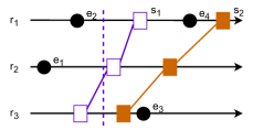
Figure 1: With space/time diagrams the events that take place on memory regions over time can be visualized. Each region is represented by an individual timeline (time passes from left to right), events are denoted as black dots and the acquisition of a memory region in a snapshot as rectangle.

2.2 Quasi-instantaneous consistency

Ottmann et al. (2022) defined the following notions of consistency. The ideal case for a snapshot is that it is taken instantaneously. In a snapshot that satisfies instantaneous consistency every memory region was copied at the same time.

Definition 1 (instantaneous consistency).

A snapshot $s$ satisfies instantaneous consistency iff all memory regions in $s$ were acquired at the same point in time. Formally:

$$\forall r,r^{\prime}\in R:s(r).t=s(r^{\prime}).t$$

If s satisfies instantaneous consistency we call s instantaneous.

When a system cannot be frozen it might still be possible to acquire a snapshot with the same contents as if it had been taken instantaneously. In this case the content is identical to an instantaneous snapshot (although not taken instantaneously) and we call such a snapshot quasi-instantaneously consistent.

Definition 2 (quasi-instantaneous consistency).

A snapshot $s$ satisfies quasi-instantaneous consistency iff the values in the snapshot could have also been acquired with an instantaneous snapshot $s^{\prime}$. Formally:

$$\exists s^{\prime}:s^{\prime}\textrm{is instantaneous}\mathrel{\land}(V_{s^{\prime}}=V_{s})$$

If s satisfies quasi-instantaneous consistency we call s quasi-instantaneous.

Two example snapshots are shown in Fig. 1. Snapshot $s_{1}$ is quasi-instantaneous since an instantaneous snapshot can be found that would have had the same contents. Such an instantaneous snapshot could have been taken right after event $e_{2}$ took place and is indicated by a dashed vertical line. For the second snapshot, $s_{2}$, on the other hand, it is not possible to construct an instantaneous snapshot with the same contents. The reason is that event $e_{3}$ happened before $e_{4}$ but in the snapshot the changes made by $e_{3}$ cannot be seen while those made by $e_{4}$ are included. Thus, snapshot $s_{2}$ is not quasi-instantaneous.

3 Observing Quasi-Instantaneous Consistency

Our approach to observe quasi-instantaneous consistency is based on the observation of consistency indicators within the snapshot. Oftentimes, such indicators already exist as part of the running system. For example, kernel data structures that save redundant information can serve as indicators (Pagani et al., 2019). However, artificial consistency indicators can also be deployed as part of general forensic readiness procedures or within the memory management of individual processes.

3.1 Current time and time of last event

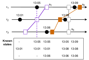
Figure 2: Knowledge about the times at which events occurred on memory regions allows to determine if a snapshot is quasi-instantaneous. Given a snapshot, a vector of the times at which the last event relative to the snapshot occurred can be formed. If this vector matches one of the known sates, the snapshot is quasi-instantaneous.

If we want to know exactly in which memory regions inconsistent contents are located, knowledge about previous states of the memory contents is necessary. An example is shown in Fig. 2 where events happen in real-time and the timestamps of events are recorded in a table shown below the space/time diagram. Note, such a data structure of all event timestamps enumerates all possible instantaneous snapshots since memory contents only change through events. For example, the instantaneous snapshot taken right after the event at 13:08, $s_{3}$ in the figure, would contain data as changed by the events at 13:05 (on region $r_{1}$), 13:08 (on region $r_{2}$) and 13:06 (on region $r_{3}$).

To identify if a snapshot is quasi-instantaneous, we need to find the “matching” instantaneous snapshot in the list of all instantaneous snapshots described above. To do this, we can either “scan” the data structure from beginning to end, or search in the vicinity of the timestamps that are stored in the snapshot. For a more specific search, the ability to determine the time of the last event on each memory region relative to the time at which the snapshot was taken on that region is helpful. For example, for snapshot $s_{1}$, the time of the most recent event on $r_{1}$ is 13:05. If the vector of these time stamps matches one of the possible instantaneous snapshots listed in the data structure, the snapshot is quasi-instantaneously consistent.

To illustrate the idea, Fig. 2 depicts two snapshots $s_{1}$ and $s_{2}$; $s_{1}$ is quasi-instantaneous since the vector of the last events matches the known state added at time 13:05. For $s_{2}$ the searched vector is {13:09, 13:01, 13:06}. Since this state is not contained in the known state array, the snapshot is not quasi-instantaneous.

3.2 Two-dimensional global counter array

We formalize this idea based on state information stored in unique counters saved at each memory region access in a global structure, the global counter array, and the region itself. The global counter array can be implemented in different variations. We introduce the general idea first, followed by a variant of the global counter array that carries redundant information helpful for visualization.

Global counter array

The global counter array $G$ is a two-dimensional array $R\times T$. As defined in section 2.1 $T=\mathbb{N}$. It contains a row for each $r\in R$. Its rows and columns are initialized with zero. Since $T$ is infinite, theoretically, $G$ is also an infinite data structure. However, at any finite point in time $G$ is also finite.

The current column to write to in $G$ is identified using the current logical time $t\in\mathbb{N}$. It is initialized with zero. Algorithm 1 shows the sequence of actions triggered by an event $e$ on $r_{i}$. When a memory region $r_{i}$ is accessed the time $t$ is incremented by one and a value $x$ written to $G$ at the index $t$: $G[r_{i}][t]:=x$. The value $x$ is dependent on the implementation variant chosen for the global counter array as we will see later. The time $t$ is saved in the memory region $r_{i}$ on which the event occurred.

Algorithm 1 Sequence of actions triggered by an event $e$ on memory region $r_{i}$

Upon Event $e$ on $r_{i}$

     $t:=t+1$

     $G[r_{i}][t]:=x$

     Save $t$ in $r_{i}$

Current time

We denote the vector $G_{t}$ which contains the index of the last visible status update for each $r$ in the global counter array $G$ at a logical point in time $t$ the current time of $t$. The value in the vector at index $i$ is returned by $G_{t}[i]$.

Figure 3: Each time an event happens on a memory region $r_{i}$, $t$ is increased by one and its value written to the appropriate row $r_{i}$ in the global counter array $G$.

3.3 Carry along global counter array

One possibility for keeping track of coexistent states is to save the value of $t$ for each event on a region $r$ in $G$ and carrying along the last visible counter updates for all other regions. Obviously, this representation is also a direct representation of all possible instantaneous snapshots with logical time.

When an event $e$ occurs on memory region $r_{i}$, the sequence of actions shown in Algorithm 1 is followed: First, the time $t$ is incremented by one. The value $x$ is written to $G$ at the index $t$, i.e., $t$: $G[r_{i}][t]:=t$. Then the time $t$ is saved in $r_{i}$ as well. Additionally, for all other $r$, the value at index $t-1$ is written to $G$, thereby carrying along the values of previous updates: $G[r_{i}][t]:=G[r_{i}][t-1],\forall r\in R:r\neq e.r$. An example of how $G$ is updated for each event is shown in Fig. 3.

Current time

The current time for a logical point in time $t$ is reconstructed from the values for each row in $G$ at index $t$: $G_{t}:={G[r_{1}][t],\ldots,G[r_{n}][t]}$. For example, the current time in Fig. 3 at time $t=5$ is $G_{t}=(1,5,4)$. This time can be used to check for quasi-instantaneous consistency, as we now explain.

4 Checking Quasi-Instantaneous Consistency

The question is how to verify if a snapshot is quasi-instantaneously consistent. For this purpose, it needs to be determined if a point in time exists at which the same contents were coexistent in memory as in the snapshot. Comparing the last point in time saved in each memory region to the states saved in the global counter array allows us to do this.

Given that the value of each memory region $r$ in the snapshot $s$ is defined by the last event that occurred on the region, each $s$ is equivalent in its values to the normalized snapshot $N(s)$, which is taken right after the occurrence of the last event for each memory region $r$ from the point of view of $s$. Fig. 4 shows an example of a snapshot and its normalized form.

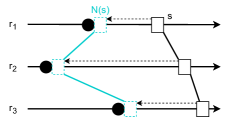
Figure 4: Given a snapshot $s$, its normalized form $N(s)$ contains the same time stamps as a snapshot which copied each memory region at the moment the last event from the perspective of $s$ had happened on it.

Definition 3 (Normalized snapshot $N(s)$).

For $r\in R$, we define $t^{\prime}_{r}$ as the point in time at which the last event relative to a snapshot $s$ was executed on $r$: $t^{\prime}_{r}:=\max(\{0\}\cup\{i\leq s(r).t\;|\;e_{i}.r=r\})$. For each memory region $r$ the snapshot $N(s)$ contains the appropriate point in time $t^{\prime}_{r}$ and the value saved in the memory region at point in time $t^{\prime}_{r}$: $N(s)(r):=(t^{\prime}_{r},m(r,t^{\prime}_{r}))$.

Proposition 4.

The values of $N(s)$ and $s$ are equivalent: $V_{N(s)}=V_{s}$

Proof.

We want to show that $\forall r\in R:N(s)(r).v=s(r).v$.

Fix an $r\in R$ and let $t:=s(r).t$. The case $t^{\prime}_{r}=t$ is trivial, since then $m(r,t^{\prime}_{r})=m(r,t)$ by assumption. As such, $V_{N(s)}=V_{s}$.

Consider $t^{\prime}_{r}<t$. If we assume $m(r,t^{\prime}_{r})\neq m(r,t)$, an event $e_{z}$ occurs after $t^{\prime}_{r}$ at time $z$: $e_{z}.r=r$ and $t^{\prime}_{r}<z\leq t$. It follows that $z\in\{i\leq s(r).t\;|\;e_{i}.r=r\}$, but then $t^{\prime}_{r}$ is not the time at which the last event happened on region $r$, since $z>t^{\prime}_{r}$. This contradicts the definition of $N(s)$. Hence, $m(r,t^{\prime}_{r})=m(r,t)$ and $V_{N(s)}=V_{s}$ accordingly.

∎

Thus, when looking at a snapshot $s$, it is equivalent to look at $N(s)$ instead. When comparing two snapshots, $s_{1}$ and $s_{2}$, they can be substituted with $N(s_{1})$ and $N(s_{2})$, respectively. This makes comparisons easier, since the values stored in the normalized snapshots are equal iff the times are equal.

Proposition 5.

For two snapshots $s_{1}$ and $s_{2}$: $T_{N(s_{1})}=T_{N(s_{2})}\Leftrightarrow V_{N(s_{1})}=V_{N(s_{2})}$

Proof.

($\Rightarrow$) Let $T_{N(s_{1})}$ be equal to $T_{N(s_{2})}$: If for both $N(s_{1})$ and $N(s_{2})$ the time at which the last event which occurred on a region $r\in R$ is equal, $t:=N(s_{1})(r).t=N(s_{2})(r).t$, then we know that $m(r,N(s_{1})(r).t)=m(r,t)=m(r,N(s_{2})(r).t)$. As such, $V_{N(s_{1})}=V_{N(s_{2})}$.

($\Leftarrow$) Let $V_{N(s_{1})}$ be equal to $V_{N(s_{2})}$: According to Proposition 4, given an $r\in R$, we have $N(s_{1})(r).v=s_{1}(r).v=s_{2}(r).v=N(s_{2})(r).v$. We need to show $N(s_{1})(r).t=N(s_{2})(r).t$.

If the values of $s_{1}$ and $s_{2}$ are equal, $s_{1}(r).v=s_{2}(r).v$, this means $m(r,s_{1}(r).t)=m(r,s_{2}(r).t)$. Let $t_{1}:=s_{1}(r).t$, $t_{2}:=s_{2}(r).t$. W.l.o.g. $t_{1}<t_{2}$. Then an $n\in\mathbb{N}$ exists for which $t_{2}=t_{1}+n$. Since $m(r,t_{1})=m(r,t_{2})$, there has been no $e_{k}$ where $t_{1}<k\leq t_{1}+n$ with $e_{k}.r=r$.

Then the sets $\{i\leq t_{1}\ |\ e_{i}.r=r\}$ and $\{i\leq t_{1}+n\ |\ e_{i}.r=r\}$ are equal, the latter of course being $\{i\leq t_{2}\ |\ e_{i}.r=r\}$. Now $N(s_{1})(r).t=max\{\{0\}\cup\{i\leq t_{1}\ |\ e_{i}.r=r\}\}=max\{\{0\}\cup\{i\leq t_{2}\ |\ e_{i}.r=r\}\}=N(s_{2})(r).t$, which completes the proof.

∎

Now that we know that for two normalized snapshots, their values are only equal iff their times are equal, the question remains how we can use this to check snapshot $s$ for quasi-instantaneous consistency. The missing piece to perform the check is the associated instantaneous snapshot of $s$, denoted $\hat{s}$. Fig. 5 shows a snapshot $s$ and its associated instantaneous snapshot $\hat{s}$ taken at the highest time found in the normalized snapshot $N(s)$.

Definition 6 (Associated instantaneous snapshot of $s$).

For a snapshot $s$, we denote by $\hat{s}$ the instantaneous snapshot at $\hat{t}_{s}$ which we call the associated instantaneous snapshot of $s$, where $\hat{t}_{s}:=\mathsf{max}(\{N(s)(r).t\;|\;r\in R\})$. Note that $T_{N(\hat{s})}=G_{\hat{t}_{s}}$.

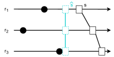
Figure 5: The associated instantaneous snapshot $\hat{s}$ of a snapshot $s$ is the instantaneous snapshot taken at the highest time of its normalized snapshot $N(s)$.

If a snapshot is equal in its values to its associated instantaneous snapshot it is quasi-instantaneously consistent. As we have established that two normalized snapshots will be equal in their values iff their times are equal, we can perform the comparison based solely on the times of the normalized snapshot of $s$, $N(s)$, and the normalized snapshot of its associated instantaneous snapshot, $N(\hat{s})$.

Theorem 7.

A snapshot $s$ is quasi-instantaneously consistent iff $T_{N(s)}=T_{N(\hat{s})}$.

Proof.

($\Rightarrow$) Given an instantaneous snapshot $s^{\prime}$ for which $V_{s^{\prime}}=V_{s}$ , we show that $T_{N(s)}=T_{N(\hat{s})}$.

Since $V_{s^{\prime}}=V_{s}$, according to Proposition 4 we can use the normalized snapshots instead: $V_{N(s^{\prime})}=V_{N(s)}$. It follows that $T_{N(s^{\prime})}=T_{N(s)}$ according to Proposition 5. Therefore $\hat{t}_{s^{\prime}}=\hat{t}_{s}$. Since there is only one instantaneous snapshot at any given time $t$, $\hat{s^{\prime}}=s^{\prime}=\hat{s}$. Thus, when we substitute $s^{\prime}$ by $\hat{s}$, $T_{N(s)}=T_{N(\hat{s})}$.

($\Leftarrow$) Given $T_{N(s)}=T_{N(\hat{s})}$ we show that a snapshot $s^{\prime}$ exists which is instantaneous and for which $V_{s^{\prime}}=V_{s}$.

Let $s^{\prime}:=\hat{s}$. By definition $\hat{s}$ is instantaneous. According to Proposition 5, $T_{N(s)}=T_{N(\hat{s})}\Rightarrow V_{N(s)}=V_{N(\hat{s})}$. Therefore, according to Proposition 4, $V_{s}=V_{\hat{s}}$.

∎

With this theorem, we have shown that we can use the normalized snapshot instead of the original snapshot to evaluate if the snapshot is quasi-instantaneously consistent or not. It also becomes apparent that comparing the time is sufficient to establish if the values of the snapshot were coexistent in memory at some point in time. Since $T_{N(\hat{s})}=G_{\hat{t}_{s}}$ it also shows how the states saved in the global counter array are used to determine existent states. Algorithm 2 summarizes how the check is performed.

Algorithm 2 Checking for quasi-instantaneous consistency

Compute $N(s)$ $\triangleright$ Extract time $t$ saved in each region

$\hat{t}_{s}:=\mathsf{max}(\{N(s)(r).t\;|\;r\in R\})$

Compute $G_{\hat{t}_{s}}$ $\triangleright$ See Algorithm 3

$T_{N_{\hat{s}}}:=G_{\hat{t}}$

if $T_{N_{\hat{s}}}=T_{N(s)}$ then

     $s$ is quasi-instantaneously consistent

else

     $s$ is not quasi-instantaneously consistent

end if

5 Improving Memory Efficiency

The implementation of the global counter array as shown in Section 3.2 is inefficient both computationally and regarding memory usage. In the following, we first show a more efficient two-dimensional implementation. As it becomes apparent that one dimension is enough to carry the necessary information, we then present a one-dimensional variant we used for implementing the global counter array.

5.1 Simplified global counter array

Looking at Fig. 3 it becomes apparent that a lot of redundant information is saved in the global counter array $G$ because the index at which $t$ is written and its value are identical. Additionally, from a practical perspective, it is more efficient to not carry along previous values of $t$. Instead, when an update of $t$ occurs a $1$ is written at index $t$ for the appropriate $r$. For all other $r$ the initial value, $0$, is not changed.

For the simplified version, an event on memory region $r_{i}$ triggers the sequence of actions shown in Algorithm 1: First, the time $t$ is incremented by one. Then, a value $x$ is written to $G$ at the index $t$, for the simplified global counter array $x$ is always $1$: $G[r_{i}][t]:=1$. Lastly, the value of $t$ is saved in $r_{i}$. Here, no additional steps are necessary. Fig. 6 shows the same sequence of events as in Fig. 3 but with the adapted implementation of $G$.

Figure 6: Each time an event happens on a memory region $r_{i}$, $t$ is increased by one and $1$ written to the according row in the global counter array $G$.

Current time

Because the last updates are not carried along, reconstructing $G_{t}$ requires to find the last update for all memory regions $r$ except the one at which a $1$ can be found in $G$ for time $t$. This can be done as shown in Algorithm 3.

Algorithm 3 Computing the current time $G_{t}$ for the logical time $t$

Initialize vector $G_{t}$ with $-1$

$t_{i}:=t$

while $\exists i:G_{t}[i]=-1$ do

     Find row $r_{h}$ where ($G[r_{h}][t_{i}]=1)\wedge(G_{t}[r_{h}]=-1)$

     $G_{t}[r_{h}]:=t_{i}$

     $t_{i}:=t_{i}-1$

     if $t_{i}=0$ then

         for all  $G_{t}[i]$ for which $G_{t}[i]=-1$ do

              $G_{t}[i]:=0$

         end for

     end if

end while

5.2 One-dimensional global counter array

The implementation variant of $G$ shown in Fig. 6 uses more memory than necessary to carry the needed information. Although at each logical point in time $t$ only one memory region is updated, for all other regions memory is reserved with only zeros entered. Since we only need to save information for exactly one region per logical point in time, we can save the known states in a list instead of a two-dimensional array. Since no second dimension exists to indicate the region at which the event occurred, this information needs to be saved in the list.

The index to write to in the one-dimensional global counter array $G$ remains the time $t$. When a memory region $r_{i}$ is accessed, $t$ is incremented and $i$ saved in $G$ at index $t$: $G[t]:=i$. The value of $t$ is saved in $r_{i}$. An example of the adapted global counter array with the same sequence of events as in the previous two examples is shown in Fig. 7.

Figure 7: Each time an event happens on a memory region $r_{i}$, $t$ is increased by one and the number of the region, $i$, written to the global counter array $G$.

Reconstructing a specific current time

To reconstruct the coexistent values at a logical point in time $t$, entries for each memory region in $G$ at or before $t$ need to be searched. If no entry for a memory region can be found no events occurred yet which means the saved value in the region equals zero. Algorithm 4 shows the detailed procedure.

Algorithm 4 Computing the current time $G_{t}$ for the logical time $t$ based on the one-dimensional global counter array

Initialize vector $G_{t}$ with $-1$

$t_{i}:=t$

while $\exists i:G_{t}[i]=-1$ do

     $r:=G[t_{i}]$

     if $G_{t}[r]=-1$ then

         $G_{t}[r]:=t_{i}$

     end if

     $t_{i}:=t_{i}-1$

     if $t_{i}=0$ then

         for all  $G_{t}[i]$ for which $G_{t}[i]=-1$ do

              $G_{t}[i]:=0$

         end for

     end if

end while

6 Evaluation

Now that we have shown that, given proper consistency indicators, theoretically quasi-instantaneous consistency can be observed, we present a practical proof-of-concept application of the method. It allows observing the quasi-instantaneous consistency of memory regions in one process. We consider two main system states for the evaluation, frozen and running. We expect that memory dumps taken of frozen systems satisfy quasi-instantaneous consistency, while those taken concurrently to the running system are expected to not (necessarily) be consistent. The evaluation is performed with a semi-automated procedure, described subsequently, which mainly differs in the method chosen to create the memory dump depending on the system state.

6.1 Procedure

For the evaluation of memory dumps taken in both system states, we use a virtual machine running Ubuntu 18.04 with 4 GB of RAM and 4 CPUs. Quasi-instantaneous consistency is observed in a specifically crafted pivot program. It meets the requirements to apply the method practically:

1. The ability to observe accesses to memory regions

2. The ability to write counter values to memory regions

3. Enough memory for the global counter array.

In the pivot program memory regions are represented by list elements and changes on them are tracked in a one-dimensional global counter array. The array is allocated with a fixed size that is sufficient to capture the events taking place during the intended runtime of the program. The changes on the list elements are performed by one or more threads. The threads randomly choose a list element to remove from the synchronized list and after a short wait reinsert the element at the beginning of the list. Each update (insertion/removal) of a list element causes an update of the time of the last event in the list element and the global counter array. The number of list elements and threads is set at the program start.

Memory dumps of the live system are taken for two different levels of activity, low and high. When creating memory dumps for the low activity level only the pivot program is executed. In comparison, the high activity level executes several other programs in parallel. This level of activity is also generated for the frozen system snapshots. Memory dumps taken in the frozen and the live system state with high activity can be summarized as follows (manually performed actions are labeled with numbers, automated actions with letters):

1. Start VM

   1. Start pivot program

   2. Mount shared folder

   3. Start grep: timeout 2m grep -r "libc" / &

   4. Retrieve meta info of pivot program (pid, heap range)

   5. Move meta info to shared folder

2. Open Firefox

3. Open YouTube, click on video

4. Open LibreOffice Writer, continuously write text

   1. Take memory dump

   2. Dump pivot program’s heap contents

The memory dump is taken approximately one minute after the grep command was executed. For all memory dumps taken without freezing the system, as a last step the heap contents of the pivot program are dumped using gdb.

Using this procedure, 30 memory dumps were created in total. Ten for the frozen system state with high activity, ten for the live system state with high activity, and ten for the live system state with low activity (details of how these memory dumps were acquired are given below). All memory dumps and analysis results, as well as the scripts used for their analyis and the source code of the pivot program are publicly available. The number of active threads in the pivot program is set to eight for high activity. The memory dumps of a live system with low activity are taken with the same timing as those with high activity but without steps (c), (2), (3), and (4), and the number of active threads in the pivot program is set to one instead of eight.

6.2 Analysis

In the analysis two types of inconsistencies are evaluated, quasi-instantaneous inconsistencies in the pivot program’s heap, and inconsistencies between numbers of virtual memory areas (VMAs) saved for each process by the kernel.

Quasi-instantaneous inconsistencies

When searching for quasi-instantaneous inconsistencies in the pivot program’s process address space, first its heap is extracted from the memory dump using the Volatility plugin linux_dump_map. Next, the list elements and the time of the last event on them as well as the global counter array are retrieved from the heap pages using a python script. In the case of the memory dumps taken without freezing the system, the global counter array is instead retrieved from the heap dump taken with gdb. This is necessary as, while in the virtual process memory the global counter array is located after the list elements and their counters, in the physical memory they might be jumbled. If the global counter array is acquired before the list elements, its contents could be not up to date with the last changes made on the list elements.

To check for violations of quasi-instantaneous consistency, we follow the steps of Algorithm 2: The time of the last event for each region is saved in a vector which is equivalent to the normalized snapshot $N(s)$. Then, the maximal time stamp in this vector $\hat{t}$ is identified, upon which the current time $G_{\hat{t}}$ is computed from the global counter array. Lastly, the normalized snapshot and the current time, i.e., the snapshot’s associated instantaneous snapshot, are compared. Should they differ in one or more values, a violation of quasi-instantaneous consistency has been identified.

VMA inconsistencies

To gain insight into inconsistencies in kernel data structures, we use a method suggested by Pagani et al. (2019). The number of VMAs assigned to each process can be retrieved from different sources, a linked list of VMAs managed for each process, a red-black tree of the VMAs, and the counter of assigned VMAs saved for each process in its task_struct structure. The Volatility plugin linux_validate_vmas retrieves the number of VMAs from the three sources and compares them. If a mismatch is detected, the name of the corresponding process and the different values are returned. The total number of processes with inconsistent VMA numbers is gathered for each dump.

6.3 Frozen system

To take a memory dump of the frozen system, we use virsh dump with option --memory-only. As this command has to be performed by the host, a script is started on the host once the shared folder has been mounted that executes the command after one minute. In the ten created memory dumps, as expected, no quasi-instantaneous or VMA inconsistencies were found. All ten snapshots were quasi-instantaneously consistent.

6.4 Running system

System state	Inconsistency type	Activity	Min	Max	Average	Affected dumps
Frozen	Quasi-instantaneous	High	0	0	0	0/10
	VMA		0	0	0	0/10
Live	Quasi-instantaneous	Low	0	3	0.8	5/10
		High	0	37	13.8	7/10
	VMA	Low	0	1	0.1	1/10
		High	3	7	4.9	9/9

Table 1: The table shows the minimum, maximum and average number of quasi-instantaneous and VMA inconsistencies found in the 30 memory dumps created for the evaluation. Out of the memory dumps taken with high system load one could not be analyzed regarding VMA inconsistencies. Therefore the average number of inconsistencies is calculated for nine instead of ten dumps.

We use LiME with option format=lime to take memory dumps of running systems. This is done from within the VM and integrated into the same script that performs the other automated tasks. For each activity (low and high), ten memory dumps were taken. The observed inconsistencies are summarized in Table 1.

For low system activity, fewer inconsistencies occurred than for high system activity. The number of memory dumps affected by quasi-instantaneous inconsistencies is higher than the number of dumps in which VMA inconsistencies were found.

With higher activity, the number of inconsistencies rises distinctly. Seven out of ten memory dumps contain quasi-instantaneous inconsistencies. Out of them one only contained two inconsistencies, the others 15 or more. The three memory dumps that contain no quasi-instantaneous inconsistencies, and the one with only two are noteworthy compared to the average number of found inconsistencies. For VMA inconsistencies a similar observation can be made. The nine memory dumps that could be analyzed regarding VMA inconsistencies, contained them. They are attributed to processes related to the web browser, audio, and gnome-shell. One memory dump had to be excluded from the VMA inconsistency check as during the check for VMA inconsistencies in this dump, the function used in the linux_validate_vmas Volatility plugin to traverse the red black tree did not return and the plugin’s execution had to be stopped. Memory dumps for which the plugin did not terminate were also observed by Pagani et al. (2019). While this is probably one symptom of inconsistencies in the memory dump, no statement about the number of VMA inconsistencies for this memory dump can be made.

7 Discussion

As expected most of the memory dumps taken on the live system with high activity are not quasi-instantaneously consistent. But the numbers vary noticeably and three memory dumps did not have inconsistencies. Using the information available through the check for quasi-instantaneous consistency, we can perform some further examinations. Given the small number of memory dumps, we do not claim that these results can be generalized to any memory acquisition but they show the advantages of using our method when investigating the reasons for inconsistencies in a memory dump.

Reconstruction of physical addresses:

While checking the heap of the pivot program for inconsistencies, the virtual addresses of the list elements and the global counter array were gathered. They are ordered sequentially on adjacent pages in the virtual memory but their mappings to physical pages do not have to be in the same order or address range. Therefore, we reconstructed to which physical pages they were mapped using Volatility’s linux_memmap plugin. From these mappings, we could reconstruct the range of physical addresses in which the list elements and the global counter array were located. This allows us to calculate the distance of each address to the nearest next address (i.e, the nearest list element). Table 2 summarizes the findings per memory dump ordered by the number of found quasi-instantaneous inconsistencies in them. Range (in pages) is the size of the physical address range in which the list elements and global counter array are located, displayed as number of pages. It is calculated by subtracting the lowest found address from the highest. The distances columns include the number of list elements that were within a 10 pages radius or directly neighbors, respectively. The largest found distance between two elements is given by Max distance. All distances are given as the number of pages (the page size is 4096 bytes).

Spread is bad:

The table supports the intuition that a longer range in which the addresses are distributed will likely lead to more inconsistencies. Or vice-versa, in memory dumps with fewer inconsistencies, more contents of interest are located on adjacent pages than in those with more inconsistencies.

Details - dump #1:

It has the highest number of inconsistencies but a relatively high number of adjacent physical addresses and not the largest range of addresses. The maximal distance between two list elements is however the largest one in the evaluated memory dumps. Taking a look at the location of the list element for which the current time was calculated reveals that it is located towards the end of the memory range and is separated by the observed largest distance from the previous 93 list elements. Thus, it is likely that there was a longer time frame during the acquisition between copying the previous elements and the last ones. Combining this with the earlier acquisition of most of the list elements, it becomes likely that updates on them are missed.

Details - dump #6:

Here, the range is the third smallest, and 85 of 101 addresses have a distance between one and ten pages but still 15 inconsistencies occurred. A closer look at the list of elements for which inconsistencies occurred in this memory dump provides a possible explanation. They are located more in the beginning of the address range with mostly smaller distances between them while the list element with the highest time stamp, i.e. the one for which the current time was identified, is located more towards the end. A big gap, 72 745 pages (the largest distance plus some smaller gaps afterward), lies between the last list element with an inconsistency and the one with the highest time stamp. Therefore, similarly to dump #1, it becomes more likely that changes on the earlier list elements occur before this list element is acquired. From the difference between the counters of the list elements for which inconsistencies were detected and their values in the current time we can also see that many updates occurred on them, the smallest number of missed updates is 42, the largest 367.

#	Inconsistencies	Range (in pages)	Distances $<=10$ pages   $\supset$	Distances $=1$ page	Max distance
1	37	224 575	61	43	103 122
2	30	423 245	47	26	79 613
3	21	141 591	20	5	54 774
4	17	150 635	33	5	53 319
5	16	267 028	44	23	82 596
6	15	79 296	85	42	71 215
7	2	99 921	81	45	55 761
8	0	82 526	76	40	62 653
9	0	12 132	75	57	3 170
10	0	4 431	97	26	2 665

Table 2: The table shows the number of quasi-instantaneous inconsistencies found in the ten memory dumps taken of the live system with high activity. For each dump the range in which the physical addresses of the 100 list elements and the global counter array are contained is given in pages. Additionally, the number of distances between the list elements and global counter array that are smaller than 11 pages and the subset of these distances that is equal to one page are shown. The last column shows the maximal observed distance between two list elements in the memory dump.

Pivot program - pros and cons:

The examples show how checking for quasi-instantaneous consistency allows gaining more insights into where content mismatches occur and how many changes on the memory regions were missed. This is currently limited to the pivot program. But the usage of the pivot program also has benefits, since its size can be chosen (for example by changing the number of list elements or their size) and the degree of activity can be manipulated by the number of threads and the frequency at which they access the list elements. As the pivot program is started as a user process, it also allows us to gather insights into the influence memory allocation strategies and fragmentation have on the process address space layout at the physical level. The different ranges and distances shown in Table 2 show that even when starting the program at approximately the same time after booting the layout varies distinctly. Should it be the goal to observe the consistency when the physical pages are located in specific page ranges, it would also be possible to remap the process’s heap pages to different physical addresses using, for example, a kernel module.

VMA inconsistencies could also be analyzed more thoroughly. For example, it would be possible to determine the addresses of the elements of the red-black tree, the elements of the VMA list, and the counter for VMAs, and judging from their relative locations it would be possible to estimate where the inconsistency could stem from, e.g., is the counter outdated or the number of elements in the list. But identifying where exactly information is missing would require more effort and may be impossible. It would also be more difficult or impossible to find out how many updates were missed exactly. The observed memory range is also limited when looking only at VMA inconsistencies.

To cover a bigger memory range having multiple indicators for content mismatches at hand would be convenient, searching for them might be eased by understanding the structures used by the operating system and their connections with each other better (Pagani and Balzarotti, 2019).

8 Conclusions and Future Work

So, finally, how can we obtain a good memory snapshot? While this is trivial for systems that can be paused (instantaneous snapshot), the situation is more complex for running ones. We, therefore, looked into the notion of quasi-instantaneous consistency which is a similar property but also works for active systems.

In this paper, we showcased a method to observe quasi-instantaneous consistency, validated it theoretically, and also demonstrated it in a case study. Our method allows assessing a portion of a memory dump for quasi-instantaneous inconsistencies based on a single memory dump. This includes locating the memory regions with inconsistencies and evaluating how many events on them were missed. A property that is useful when searching for improvements in existing memory acquisition methods. For example, identifying alternative orders of memory acquisition, comparable to the adaptations to LiME suggested by Pagani et al. (2019). Our tests then confirmed that instantaneous snapshots (frozen systems) are indeed perfect and are the method of first resort. Furthermore, for live systems, we were able to show that a high system load results in more inconsistencies. More tests are needed here, but this could potentially mean that it may be wise to close (non-relevant) applications before obtaining a snapshot on a running system.

Moving forward, the method could be used to evaluate different memory acquisition tools. Thereby, a broader data base could be built to investigate our preliminary observations further. The method for observing quasi-instantaneous consistency could also be moved to different memory ranges than the pivot program. Concerning the main memory, it would be possible to integrate it at the hypervisor level. From there the address ranges that contain contents of interest could be identified and observed. For example, the memory ranges containing structures that are necessary for the analysis, like page tables and process structures. A second consideration is alienating this method to live acquisition of hard disk contents where it could be possible to integrate it into the file system or block device drivers.

Our implementation also suffers some shortages which require attention. For instance, the pivot program utilizes a fixed-size global counter array which is not practical for larger memory regions or longer observation times. One possibility would be to implement it as a ring buffer, i.e., restarting at the beginning once the last entry has been written. This would require an overflow detection in the implementation, and in the analysis, with the latter being the more difficult task.

Acknowledgments

Work was supported by Deutsche Forschungsgemeinschaft (DFG, German Research Foundation) as part of the Research and Training Group 2475 “Cybercrime and Forensic Computing” (grant number 393541319/GRK2475/1-2019).

References

- Bauer et al. (2016) Bauer, J., Gruhn, M., Freiling, F.C., 2016. Lest we forget: Cold-boot attacks on scrambled DDR3 memory. Digit. Investig. 16 Supplement, S65–S74. URL: https://doi.org/10.1016/j.diin.2016.01.009, doi:10.1016/j.diin.2016.01.009.
- Campbell (2013) Campbell, W., 2013. Volatile memory acquisition tools – A comparison across taint and correctness, in: Proc. 11th Australian Digital Forensics Conference.
- Case and Richard III (2017) Case, A., Richard III, G.G., 2017. Memory forensics: The path forward. Digital Investigation 20, 23–33.
- Gruhn and Freiling (2016) Gruhn, M., Freiling, F.C., 2016. Evaluating atomicity, and integrity of correct memory acquisition methods. Digital Investigation 16, S1–S10.
- Halderman et al. (2009) Halderman, J.A., Schoen, S.D., Heninger, N., Clarkson, W., Paul, W., Calandrino, J.A., Feldman, A.J., Appelbaum, J., Felten, E.W., 2009. Lest we remember: cold-boot attacks on encryption keys. Commun. ACM 52, 91–98. URL: https://doi.org/10.1145/1506409.1506429, doi:10.1145/1506409.1506429.
- Inoue et al. (2011) Inoue, H., Adelstein, F., Joyce, R.A., 2011. Visualization in testing a volatile memory forensic tool. Digital Investigation 8, S42–S51.
- Kiperberg et al. (2019) Kiperberg, M., Leon, R., Resh, A., Algawi, A., Zaidenberg, N., 2019. Hypervisor-assisted atomic memory acquisition in modern systems, in: International Conference on Information Systems Security and Privacy, SCITEPRESS Science And Technology Publications.
- Lempereur et al. (2012) Lempereur, B., Merabti, M., Shi, Q., 2012. Pypette: A platform for the evaluation of live digital forensics. Int. Journal of Digital Crime and Forensics 4, 31–46.
- Martignoni et al. (2010) Martignoni, L., Fattori, A., Paleari, R., Cavallaro, L., 2010. Live and trustworthy forensic analysis of commodity production systems, in: International Workshop on Recent Advances in Intrusion Detection, Springer. pp. 297–316.
- Mattern (1989) Mattern, F., 1989. Virtual time and global states of distributed systems, in: Proceedings of the International Workshop on Parallel and Distributed Algorithms, pp. 215–226.
- Ottmann et al. (2022) Ottmann, J., Breitinger, F., Freiling, F., 2022. Defining atomicity (and integrity) for snapshots of storage in forensic computing, in: Proceedings of the Digital Forensics Research Conference Europe (DFRWS EU), Oxford.
- Pagani and Balzarotti (2019) Pagani, F., Balzarotti, D., 2019. Back to the whiteboard: a principled approach for the assessment and design of memory forensic techniques, in: USENIX Security Symposium, pp. 1751–1768.
- Pagani et al. (2019) Pagani, F., Fedorov, O., Balzarotti, D., 2019. Introducing the temporal dimension to memory forensics. ACM Transactions on Privacy and Security (TOPS) 22, 1–21.
- Vömel and Freiling (2012) Vömel, S., Freiling, F.C., 2012. Correctness, atomicity, and integrity: defining criteria for forensically-sound memory acquisition. Digital Investigation 9, 125–137.
- Vömel and Stüttgen (2013) Vömel, S., Stüttgen, J., 2013. An evaluation platform for forensic memory acquisition software. Digital Investigation 10, S30–S40.
- Yu et al. (2012) Yu, M., Qi, Z., Lin, Q., Zhong, X., Li, B., Guan, H., 2012. Vis: Virtualization enhanced live forensics acquisition for native system. Digital Investigation 9, 22–33.