The Calderón problem revisited:
Reconstruction with resonant perturbations

Abstract.

The original Calderón problem consists in recovering the potential (or the conductivity) from the knowledge of the related Neumann to Dirichlet map (or Dirichlet to Neumann map). Here, we first perturb the medium by injecting small-scaled and highly heterogeneous particles. Such particles can be bubbles or droplets in acoustics or nanoparticles in electromagnetism. They are distributed, periodically for instance, in the whole domain where we want to do reconstruction. Under critical scales between the size and contrast, these particles resonate at specific frequencies that can be well computed. Using incident frequencies that are close to such resonances, we show that

1. the corresponding Neumann to Dirichlet map of the composite converges to the one of the homogenized medium. In addition, the equivalent coefficient, which consist in the sum of the original potential and the effective coefficient, is negative valued with a controlable amplitude.

2. as the equivalent coefficient is negative valued, then we can linearize the corresponding Neumann to Dirichlet map using the effective coefficient’s amplitude.

3. from the linearized Neumann to Dirichlet map, we reconstruct the original potential using explicit complex geometrical optics solutions (CGOs).

1. Introduction and statement of the results

1.1. Introduction

The original Calderón problem stated in the acoustic framework reads as follows. Let $n:=c^{-1}$ be the index of refraction, where $c$ stands for the acoustic sound speed. In turn, this speed of sound is given by $c:=\sqrt{\dfrac{k}{\rho}}$ where $\rho$ is the mass density and $k$ is the bulk modulus. In the time-harmonic regime, the propagation of the acoustic waves is modelled by:

(1.1) $$\begin{cases}\left(\Delta+\omega^{2}\,n^{2}(\cdot)\right)\,p^{f}=0\quad\text{in}\quad\Omega,\\ \qquad\quad\qquad\,\partial_{\nu}p^{f}\;=f\;\;\;\text{on}\quad\partial\Omega.\end{cases}$$

where $p^{f}$ is the acoustic pressure generated by the applied source $f$. The Neumann to Dirichlet (NtD) operator $\Lambda_{c}$ corresponds to any $f\in H^{-\frac{1}{2}}(\partial\Omega)$, the trace on $\partial\Omega$ of the induced pressure $p^{f}$, i.e. $\Lambda_{c}(f):=p^{f}_{|_{\partial\Omega}}$. The Calderón problem consists in recovering the sound speed $c$ from the knowledge of the NtD map $\Lambda_{c}$. According to the model $(\ref{EquaKg-introdution})$, the mass density $\rho$ is assumed to be a constant, while the bulk modulus $k$ is variable in a smooth domain $\Omega$. We assume $k$ to be a $W^{1,\infty}(\Omega)$ and positive function and $\Omega$ of class $C^{2}$. In addition, we assume that $(\ref{EquaKg-introdution})$ has a unique solution, i.e. $\omega^{2}$ is not an eigenvalue of $-n^{-2}\Delta$ with zero Neumann boundary condition on $\partial\Omega$.

The Calderón problem was the object of an intensive study since the early 80’s. The reader can see the following references for more information [14], [22], [28] and [33]. A model of particular interest is the EIT (Electrical Impedance Tomography) problem, also called Calderón’s problem, which consists in identifying the conductivity $\gamma$ using Cauchy data $(u_{|_{\partial\Omega}},\gamma\nabla u\cdot\nu_{|_{\partial\Omega}})$ of the solution of equation $\nabla\cdot\gamma\nabla u=0$, in $\Omega\subset\mathbb{R}^{3}$, where $\nu$ is the outward unit normal vector to $\partial\Omega$. The uniqueness question of this problem is reduced to the construction of the so-called complex geometrical optics solutions (in short CGO’s), see [32], where $\gamma$ is a positive $C^{2}$-smooth function. The regularity of $\gamma$ is reduced to $C^{\frac{3}{2}+\epsilon},\epsilon>0$, in [4], then to $\mathbb{W}^{\frac{3}{2},\infty}$ in [27] and to $\mathbb{W}^{\frac{3}{2},p},p>6$ in [7]. Finally, in [12] and [19] this condition is reduced to $W^{1,\infty}$ and then to $W^{1,3}$ in [20]. The corresponding Calderón problem in the 2D-setting was solved in [25]. In [9] the author shows, for the Schrödinger equation given by $\Delta u+\mathfrak{q}\,u=0$, in $\Omega\subset\mathbb{R}^{2}$, the uniqueness of a reconstruction of the potential $\mathfrak{q}(\cdot)\in\mathbb{L}^{p}\left(\Omega\right),p>2,$ from the Cauchy data, i.e. $\left(u_{|_{\partial\Omega}};\partial_{\nu}u_{|_{\partial\Omega}}\right)$, see [9, Theorem 3.5]. In [25], we find a justification of the uniquely determination, from the knowledge of Dirichlet-to-Neumann map, of the coefficient $\gamma$ of the elliptic equation $\nabla\cdot\left(\gamma\,\nabla u\right)=0$ in a two dimensional domain. In [11], it is proved that if for all cubes $\bm{Q}\subset\mathbb{R}^{n}$ the condition on the smallness of $\underset{\bm{Q}}{Sup}\;\left|\bm{Q}\right|^{\frac{2\,p\,-\,n}{n\,p}}\;\left\|\mathfrak{q}\right\|_{\mathbb{L}^{p}(\bm{Q})},\quad p>\frac{(n-1)}{2},$ is satisfied, or $\mathfrak{q}\in\mathbb{L}^{p}$ with $p>\frac{n}{2}$, then the Dirichlet-to-Neumann map determines the potential $\mathfrak{q}$. Let us also cite [24, 13] regarding Dirac-type singular potentials. For more details, and without being exhaustive we refer the readers to the following works [1, 2, 27, 6, 8, 32, 23, 26, 29] and the references therein. Let us mention, however, that apart from few works, like [26], where we find a reconstruction algorithm, most of these works are devoted to unique identifiability questions or stability estimates.

In this work, we propose a different approach for solving re-constructively this problem. We are inspired by our recent works on using resonant contrast agents for solving inverse problems appearing in some imaging modalities, ultrasound, optics or photo-acoustic imaging modalities, [17, 16, 18, 15, 31, 30]. In those works, we use the measurements created after injecting single contrast agents (acoustic bubbles or nano-particles) as follows:

1. In the time-harmonic regime, we recover the induced resonances (as the Minnaert or plasmonic ones) from which, we could recover the wave speeds (or related coefficients), see [17, 16, 15].

2. In the time-domain regime, we recover the internal values of the travel time function. From the Eikonal equation, we extract the values of the speed, see [18, 31, 30].

In those works, we use contrast agents injected in isolation. This means, for each single injected agent we collect the generated measurements. However, it is of importance to emphasize that we measure only on one single point. In terms of dimensionality, this is advantageous.

In the current work, we inject the contrast agents all at once and then collect the measurements for multiple incident waves. In short, we collect the NtD mapping after injecting the collection of contrast agents all at once. With such measurements, we propose an approach how to do the reconstruction of the sound speed $c(\cdot)$. This approach is divided into two steps:

1. In the first step, we show that the NtD map generated by the coefficient $n^{2}(\cdot)$ and the collection of contrast agents converges to the one generated by a sum of $n^{2}(\cdot)$ and an effective coefficient. This effective coefficient is negative values and one can tune its amplitude. The negativity of the effective coefficient, which is key, is due to the resonant character of the injected contrast agents. Therefore, we can tune these injected agents so that the sum of $n^{2}(\cdot)$ and the effective coefficients is negative valued with a controllable amplitude.

2. From the effective NtD map, we reconstruct the coefficient $n^{2}(\cdot)$. To do so, we show that, due to the negativity of the effective coefficients, mentioned above, we can linearize the effective NtD map. Finally, from this linearized map, we derive an explicit formula to recover $n^{2}(\cdot)$ in terms of (explicit) CGO-solutions.

To go more in details, let us take as contrast agents droplets, which are bubbles filled in with water, having the following properties. They are modelled as $D_{j},j=1,...,M,$ of the form $D_{j}=z_{j}+a\;B$ with $B$ as a smooth domain containing the origin and maximum radius as unity, such that $D=\underset{j=1}{\overset{M}{\cup}}D_{j}$. Their mass density $\rho_{j}$ are equal and estimated as $\rho_{j}=\rho_{0}\neq 1$, for $1\leq j\leq M$, with $\rho_{0}$ is a constant independent on the parameter $a$, while their bulk modulus are very small and of order

(1.2) $$k_{j}=k_{0}\;a^{2},$$

with $k_{0}$ being as fixed constant independent of $a$. The maximum radius $a$ of this droplet is of order micrometer, therefore we take

$$a\ll 1.$$

We introduce the Newtonian operator $N_{D_{j}}^{\phi}:\mathbb{L}^{2}(D_{j})\rightarrow\mathbb{L}^{2}(D_{j})$ with the image in $\mathbb{H}^{2}(D_{j})$ given by the expression

(1.3) $$N_{D_{j}}^{\phi}(f)(x):=\int_{D_{j}}\phi(x;y)\;f(y)\;dy,\;x\in D_{j},$$

where $\phi(\cdot;\cdot)$ is the fundamental solution of the interior Neumann problem for the Laplace’s equation, such that

(1.4) $$\begin{cases}\Delta\phi=-\,\delta\quad\text{in}\quad\Omega\\ \partial_{\nu}\phi=\;\;\;0\;\;\;\text{on}\;\;\partial\Omega\end{cases}.$$

This operator is self-adjoint and compact, therefore it enjoys a positive sequence of eigenvalues $\left\{\lambda^{D_{j}}_{n}\right\}_{n\in\mathbb{N}}$ and they scale as $\lambda^{D_{j}}_{n}=a^{2}\;\lambda^{B}_{n}$. We fix any $n_{0}\in\mathbb{N}$; $j\in\{1;\cdots;M\}$ and we consider the eigenvalue $\lambda^{D_{j}}_{n_{0}}$. The incident frequency $\omega$ that we use, in this acoustic model, is taken of the form:

(1.5) $$\frac{\omega^{2}}{\omega_{0}^{2}}=1-\frac{c_{n_{0}}\;a^{h}}{k_{0}}$$

with $c_{n_{0}}\in\mathbb{R}$,

(1.6) $$c_{n_{0}}<0,$$

is a parameter which is independent of $a$. The quantity $\omega_{0}$ is defined as

$$\omega_{0}:=\sqrt{\frac{k_{j}}{\lambda^{D_{j}}_{n_{0}}}}=\sqrt{\frac{k_{0}}{\lambda^{B}_{n_{0}}}},$$

where the last equality is a consequence of the eigenvalues scales and $(\ref{ScaleBulk})$.

The droplets are distributed periodically inside $\Omega$. We are concerned with the case where we have the number $M$ of droplets of the order

(1.7) $$M\sim a^{h-1},\;a\ll 1\quad\text{with}\quad 0\leq h<1,$$

and, then, the minimum distance between the droplets is

$$d:=\underset{i\neq j\atop 1\leq i,j\leq M}{\min}\left|z_{i}-z_{j}\right|\sim a^{\frac{(1-h)}{3}},\;a\ll 1\quad\text{with}\quad 0\leq h<1,$$

as $M\sim d^{-3}$.

1.2. From the original NtD map $\Lambda_{D}$ to the effective NtD map $\Lambda_{P}$

Let $v^{g}(\cdot)$ to be solution of

(1.8) $$\begin{cases}\left(\Delta+\omega^{2}\,n^{2}(\cdot)+\omega^{2}\,\dfrac{\rho_{1}}{k_{1}}\,\underset{D}{\chi}\right)\,v^{g}=0\quad\text{in}\quad\Omega,\\ \qquad\quad\;\,\qquad\qquad\qquad\;\quad\partial_{\nu}v^{g}=g\quad\text{on}\quad\partial\Omega.\end{cases}$$

Multiplying $(\ref{Equavf})$ by $p^{f}(\cdot)$, solution of $(\ref{EquaKg-introdution})$, and integrating over $\Omega$, we obtain

$$\langle\Lambda_{0}\left(f\right);g\rangle_{\mathbb{H}^{\frac{1}{2}}(\partial\Omega)\times\mathbb{H}^{-\frac{1}{2}}(\partial\Omega)}=\langle\nabla v^{g};\nabla p^{f}\rangle_{\mathbb{L}^{2}(\Omega)}-\omega^{2}\,\langle n^{2}\,v^{g};p^{f}\rangle_{\mathbb{L}^{2}(\Omega)}-\omega^{2}\,\dfrac{\rho_{1}}{k_{1}}\,\langle v^{g};p^{f}\rangle_{\mathbb{L}^{2}(D)},$$

where $\Lambda_{0}$ is the NtD map defined from $\mathbb{H}^{-\frac{1}{2}}\left(\partial\Omega\right)$ to $\mathbb{H}^{\frac{1}{2}}\left(\partial\Omega\right)$ by

$$\langle\Lambda_{0}\left(f\right);g\rangle_{\mathbb{H}^{\frac{1}{2}}(\partial\Omega)\times\mathbb{H}^{-\frac{1}{2}}(\partial\Omega)}:=\int_{\partial\Omega}p^{f}(x)\,g(x)\,d\sigma(x).$$

Hence, if we set $\Lambda_{D}$ to be the NtD map of the background after injecting a cluster of droplets, we end up with the coming formula

(1.9) $$\langle\Lambda_{D}(f);g\rangle_{\mathbb{H}^{\frac{1}{2}}(\partial\Omega)\times\mathbb{H}^{-\frac{1}{2}}(\partial\Omega)}-\langle\Lambda_{0}\left(f\right);g\rangle_{\mathbb{H}^{\frac{1}{2}}(\partial\Omega)\times\mathbb{H}^{-\frac{1}{2}}(\partial\Omega)}=\omega^{2}\,\dfrac{\rho_{1}}{k_{1}}\;\langle v^{g};p^{f}\rangle_{\mathbb{L}^{2}(D)},$$

where

$$\langle\Lambda_{D}(f);g\rangle_{\mathbb{H}^{\frac{1}{2}}(\partial\Omega)\times\mathbb{H}^{-\frac{1}{2}}(\partial\Omega)}:=\langle\nabla v^{g};\nabla p^{f}\rangle_{\mathbb{L}^{2}(\Omega)}-\omega^{2}\,\langle n^{2}\,v^{g};p^{f}\rangle_{\mathbb{L}^{2}(\Omega)}.$$

In a similar way, we define $u^{g}(\cdot)$ to be solution of

(1.10) $$\begin{cases}\left(\Delta+\omega^{2}\,n^{2}(\cdot)-P^{2}\right)\,u^{g}\;=0\quad\text{in}\quad\Omega,\\ \qquad\qquad\qquad\qquad\partial_{\nu}u^{g}\;=g\;\;\;\text{on}\quad\partial\Omega.\end{cases}$$

Here

(1.11) $$P^{2}:=\frac{-\,k_{0}\;\left(\langle 1;\overline{e}_{n_{0}}\rangle_{\mathbb{L}^{2}(B)}\right)^{2}}{\lambda_{n_{0}}^{B}\;c_{n_{0}}},$$

where $\overline{e}_{n_{0}}$ is the eigenfunction associated to the eigenvalue $\lambda_{n_{0}}^{B}$ related to the Newtonian operator, given by $(\ref{DefNPO})$, defined in the domain $B$. Multiplying $(\ref{EquaWf})$ by $p^{f}(\cdot)$, solution of $(\ref{EquaKg-introdution})$, and integrating over $\Omega$, we obtain

$$\langle\Lambda_{0}\left(f\right);g\rangle_{\mathbb{H}^{\frac{1}{2}}(\partial\Omega)\times\mathbb{H}^{-\frac{1}{2}}(\partial\Omega)}=\langle\nabla u^{g};\nabla p^{f}\rangle_{\mathbb{L}^{2}(\Omega)}-\omega^{2}\,\langle n^{2}\,u^{g};p^{f}\rangle_{\mathbb{L}^{2}(\Omega)}+P^{2}\,\langle u^{g};p^{f}\rangle_{\mathbb{L}^{2}(\Omega)}.$$

Hence, if we set $\Lambda_{P}$ to be the NtD map of the equivalent background, we obtain

(1.12) $$\langle\Lambda_{P}(f);g\rangle_{\mathbb{H}^{\frac{1}{2}}(\partial\Omega)\times\mathbb{H}^{-\frac{1}{2}}(\partial\Omega)}-\langle\Lambda_{0}\left(f\right);g\rangle_{\mathbb{H}^{\frac{1}{2}}(\partial\Omega)\times\mathbb{H}^{-\frac{1}{2}}(\partial\Omega)}=-\,P^{2}\,\langle u^{g};p^{f}\rangle_{\mathbb{L}^{2}(\Omega)},$$

where

$$\langle\Lambda_{P}(f);g\rangle_{\mathbb{H}^{\frac{1}{2}}(\partial\Omega)\times\mathbb{H}^{-\frac{1}{2}}(\partial\Omega)}:=\langle\nabla u^{g};\nabla p^{f}\rangle_{\mathbb{L}^{2}(\Omega)}-\omega^{2}\,\langle n^{2}\,u^{g};p^{f}\rangle_{\mathbb{L}^{2}(\Omega)}.$$

From $(\ref{Equa1Lambda})$ and $(\ref{Equa2Lambda})$, we see that

(1.13) $$\langle\Lambda_{D}(f);g\rangle_{\mathbb{H}^{\frac{1}{2}}(\partial\Omega)\times\mathbb{H}^{-\frac{1}{2}}(\partial\Omega)}-\langle\Lambda_{P}(f);g\rangle_{\mathbb{H}^{\frac{1}{2}}(\partial\Omega)\times\mathbb{H}^{-\frac{1}{2}}(\partial\Omega)}=\omega^{2}\,\dfrac{\rho_{1}}{k_{1}}\,\langle v^{g};p^{f}\rangle_{\mathbb{L}^{2}(D)}\,+\,P^{2}\,\langle u^{g};p^{f}\rangle_{\mathbb{L}^{2}(\Omega)}.$$

In the sequel, we prove that when $M$ is large, or $a$ is small, the perturbed medium, after injecting a cluster of $M$ droplets, behaves like the equivalent background. In other words, the map $\Lambda_{D}$ converges to $\Lambda_{p}$.

Theorem 1.1.

We have the following convergence

$$\langle\Lambda_{D}(f);g\rangle_{\mathbb{H}^{\frac{1}{2}}(\partial\Omega)\times\mathbb{H}^{-\frac{1}{2}}(\partial\Omega)}\underset{a\rightarrow 0}{\longrightarrow}\langle\Lambda_{P}(f);g\rangle_{\mathbb{H}^{\frac{1}{2}}(\partial\Omega)\times\mathbb{H}^{-\frac{1}{2}}(\partial\Omega)},$$

uniformly in terms of $\left(f,g\right)\in\mathbb{H}^{-\frac{1}{2}}\left(\partial\Omega\right)\times\mathbb{H}^{-\frac{1}{2}}\left(\partial\Omega\right)$. Precisely, we have the following rate

(1.14) $$\left\|\Lambda_{D}-\Lambda_{P}\right\|_{\mathcal{L}(\mathbb{H}^{-\frac{1}{2}}(\partial\Omega),\mathbb{H}^{\frac{1}{2}}(\partial\Omega))}\lesssim a^{\frac{(1-h)(1-\delta)}{3(3-\delta)}}\,P^{2},\;a\ll 1,$$

where $\delta$ a sufficiently small but arbitrarily positive number.

Remark 1.2.

Two comments are in order.

2. Since $M\sim a^{h-1}$ and $\delta$ is very small, we can rewrite $(\ref{energy-D})$ as:

   $$\left\|\Lambda_{D}-\Lambda_{P}\right\|_{\mathcal{L}(\mathbb{H}^{-\frac{1}{2}}(\partial\Omega),\mathbb{H}^{\frac{1}{2}}(\partial\Omega))}\lesssim M^{\frac{(\delta-1)}{3(3-\delta)}}\,P^{2},\;M\gg 1.$$

   We can choose $M$, i.e. $a$, such that

   (1.15) $$M^{\frac{(\delta-1)}{3(3-\delta)}}\,P^{2}\ll 1.$$

4. The parameter $\delta$ in $(\ref{energy-D})$ is linked to the $\mathbb{L}^{3-\delta}(\Omega)$-integrability of the fundamental solution $\phi(\cdot;\cdot)$, solution of $(\ref{phi-harmonic})$. Additional details can be found in Lemma 4.2 and its associated proof given in Subsection 6.2.

As we assume to know the NtD map $\Lambda_{D}$, for $M$ large, the previous theorem suggests the following result.

Corollary 1.3.

The NtD map $\Lambda_{P}$ is approximately known.

The proof of Theorem 1.1 is based on the point-interaction approximation, or the so-called Foldy-Lax approximation. We first approximate the left part in (1.14) by a linear combination of elements of a vector which is solution of an algebraic system. This algebraic system captures the multiple scattering between the injected droplets through an interaction matrix where the interaction coefficients, that are also called scattering coefficients, are all positive due to the choice made in (1.5) of the sign of $c_{n_{0}}$. To prove the invertibility of this algebraic system, uniformly of the large number $M$ of droplets, we first justify the invertibility of the related continuous integral equation and then, we show, with quite tedious computations, that the algebraic equation is ’a discrete form’ of this continuous integral equation.

Remark 1.4.

Two remarks are in order.

1. In $(\ref{DefP2cn0})$, we take the constant $c_{n_{0}}<0$ and the parameter $P^{2}$ such that

   $$P^{2}>\omega_{0}^{2}\;\left\|n^{2}\right\|_{\mathbb{L}^{\infty}(\Omega)}:=P_{\min},$$

   where $\omega_{0}^{2}=\dfrac{k_{0}}{\lambda^{B}_{n_{0}}}$. This is possible if we choose the parameter $c_{n_{0}}$ to satisfies

   $$-\,\rho^{-1}\,\underset{y\in\Omega}{Inf}\left|k(y)\right|\,\left(\langle 1;\overline{e}_{n_{0}}\rangle_{\mathbb{L}^{2}(B)}\right)^{2}\,<\,c_{n_{0}}\,<\,0\quad\text{and}\quad c_{n_{0}}\rightarrow 0^{-}.$$

   We recall that the parameter $c_{n_{0}}$ appears in (1.5) and we have (1.11). The coefficient $c_{n_{0}}$ is taken small, and hence $P$ large, but satisfies (1.15).

2. The parameter $h$ appearing in (1.5) models how dilute, or dense, is the distribution of the injected droplets in $\Omega$. If $h$ is close to $1$, we have a dense distribution and when $h$ is close to $0$ we have a light distribution.

1.3. The linearization of $\Lambda_{P}$

Theorem 1.5.

We have the following linearisation of $\Lambda_{P}$, in the $\mathbb{H}^{\frac{1}{2}}(\partial\Omega)$ sense,

(1.16) $$\Lambda_{P}(f)-q^{f}=\omega^{2}\,\gamma\left(\bm{W}^{q^{f}}\right)+\mathcal{O}\left(\left\|f\right\|_{\mathbb{H}^{-\frac{1}{2}}(\partial\Omega)}\,\frac{1}{P^{4}}\right),$$

where $f\in\mathbb{H}^{-\frac{1}{2}}(\partial\Omega)$,   $q^{f}$ is solution of

(1.17) $$\begin{cases}\left(\Delta-P^{2}\right)q^{f}=0\quad\,\text{in}\quad\Omega,\\ \qquad\;\,\quad\partial_{\nu}q^{f}=f\quad\text{on}\quad\partial\Omega,\end{cases}$$

and $\bm{W}^{q^{f}}$ satisfies

$$\begin{cases}\left(\Delta-P^{2}\,I\right)\bm{W}^{q^{f}}\,=-\,n^{2}\,q^{f}\quad\text{in}\quad\Omega,\\ \qquad\qquad\,\partial_{\nu}\bm{W}^{q^{f}}=0\quad\quad\;\quad\text{on}\quad\partial\Omega.\end{cases}$$

Therefore knowing $\Lambda_{P}(f)$ allows us to construct $\bm{W}^{q^{f}}$, for $f\in\mathbb{H}^{-\frac{1}{2}}(\partial\Omega)$.

The proof of Theorem 1.5 is based on the observation that the solution operator (i.e. the Lippmann-Schwinger operator) of the problem (1.10) can be seen as the one of the problem (1.17) plus a ’small’ perturbation. The smallness of this perturbation permits us to justify the related linearization. The arguments of the analysis are based on the spectral and scaling properties of the Newtonian operator of the solution operator of (1.17) via Calderon-Zygmund type estimates.

1.4. Construction of $c(\cdot)$ from the linearization of $\Lambda_{P}$

The next theorem describes a way how we can reconstruct the sound speed from the linearized part of $\Lambda_{P}$.

Theorem 1.6.

For every $l:=\left(l_{1};l_{2};l_{3}\right)\in\mathbb{Z}^{3}$, we choose

(1.18) $$\xi=\frac{P^{2+\varsigma}\,\left|l\right|^{2+\varsigma}}{\sqrt{2}\,\sqrt{l^{2}_{2}+l^{2}_{3}}}\;\begin{pmatrix}-i\left(l_{2}^{2}+l_{3}^{2}\right)\\ -\left|l\right|\,l_{3}+i\,l_{1}\,l_{2}\\ -\left|l\right|\,l_{2}+i\,l_{1}\,l_{3}\end{pmatrix},\text{with}\;\;\varsigma\in\mathbb{R}^{+}.$$

Hence,

(1.19) $$\left|\xi\right|=P^{2+\varsigma}\,\left|l\right|^{3+\varsigma}.$$

We set $q^{f}(\cdot):=q^{l,\xi}$ the function defined by

$$q^{l,\xi}(x):=e^{i\,\xi\cdot x}\,\left(e^{i\,x\cdot l}\,+r_{1}(x)\right),\quad x\in\mathbb{R}^{3},$$

and $r_{1}(\cdot)$ is such that

(1.20) $$\left(\Delta+2\,i\,\xi\cdot\nabla-P^{2}\right)r_{1}(x)=\left(\left|l\right|^{2}+P^{2}\right)\;e^{i\,x\cdot l},\quad\text{in}\quad\Omega.$$

In the same manner we set $q^{g}(\cdot):=q^{\xi}(\cdot)$ to be the function defined by

$$q^{\xi}(x):=e^{-i\,\xi\cdot x}\left(1+r_{2}(x)\right),\quad x\in\mathbb{R}^{3},$$

where $r_{2}(\cdot)$ is such that

(1.21) $$\left(-\Delta+2\,i\,\xi\cdot\nabla+P^{2}\right)r_{2}(x)=-\,P^{2}\;,\quad\text{in}\quad\Omega.$$

Then we have the following approximate reconstruction formula:

(1.22) $$n^{2}(x)=\left(2\,\pi\right)^{-3}\;\sum_{\ell\in\mathbb{Z}^{3}}\langle\bm{W}^{q^{l,\xi}};\partial_{\nu}q^{\xi}\;\rangle\;\;e^{i\,\ell\cdot x}+\mathcal{O}\left(P^{-\varsigma}\right),$$

in the $L^{2}(\Omega)$ sense.

The justification of the existence and uniqueness of solutions corresponding to the problems $(\ref{DiffEquar1Intro})$ and $(\ref{DiffEquar2Intro})$ can be found in [29, Section 3.2]. More precisely, in [29, Theorem 3.7] the result is proved first for the free case equation, i.e. equation of the form $\left(\Delta+2\,i\,\xi\cdot\nabla\right)r=f$, where $r(\cdot)$ is a correction term and $f$ is a source data. Then, in [29, Theorem 3.8] the general case, i.e. equation of the form $\left(\Delta+2\,i\,\xi\cdot\nabla+\textbf{q}\right)r=f$, where q is a potential, was proved under the conditions $\xi\cdot\xi=0\quad\text{and}\quad\left|\xi\right|\geq\max\left(C_{0}\,\left\|\textbf{q}\right\|_{\mathbb{L}^{\infty}(\Omega)};1\right)$, where $C_{0}$ is a constant depending on the domain $\Omega$ and the space dimension. These nicely rederived estimates are proved originally in the seminal work [32, Theorem 1.1, Proposition 2.1].

The key observation here is that these CGOs are solutions of fully explicit equations, see (1.20) and (1.21), which make the representation in (1.22) re-constructive.

The remaining parts of the paper are organized as follows. In Section 2, we discuss and justify the linearization step and in Section 3 we deal with the reconstruction of $n^{2}(\cdot)$ from the linearized NtD map. The justification of the effective NtD is stated in Section 4. This choice is taken as this step is, technically, the most involved part. Section 5 is devoted to the proof of the invertibility of the algebraic system related to the derivation of the effective NtD map. Finally, we postpone several technical steps to be developed and justified in Section 6 stated as an appendix.

2. Linearization of $\Lambda_{P}$ - Proof of Theorem 1.5

Let $u^{f}(\cdot)$ be the solution of the following Lippmann-Schwinger Equation (L.S.E in short)

(2.1) $$u^{f}(x)-\omega^{2}\,N^{p}\left(n^{2}\,u^{f}\right)(x)\,=q^{f}(x),\quad x\in\Omega,$$

where $q^{f}(\cdot)$ is solution of $(\ref{Equaqf})$ and $G_{p}(\cdot,\cdot)$ satisfies

$$\begin{cases}\left(\Delta-P^{2}\right)G_{p}(\cdot,\cdot)=-\,\delta\quad\text{in}\quad\Omega,\\ \qquad\;\quad\partial_{\nu}G_{p}(\cdot,\cdot)=0\qquad\text{on}\quad\partial\Omega.\end{cases}$$

In effortless manner we can check that $u^{f}(\cdot)$, solution of $(\ref{UfLSE})$, is also solution of $(\ref{EquaWf})$. Moreover, by an induction process on the L.S.E, given by $(\ref{UfLSE})$, we prove that

(2.2) $$u^{f}(x)-q^{f}(x)=\omega^{2}\,\gamma N^{p}\left(n^{2}\,q^{f}\right)(x)+\sum_{j\geq 2}\left(K_{j}\overset{j}{\otimes}\left(n^{2}\right)\right)(x),\quad x\in\partial\Omega,$$

where

$$\left(K_{2}\overset{2}{\otimes}\left(n^{2}\right)\right)(x) = \left(\omega^{2}\right)^{2}\,\gamma N^{p}\left(n^{2}\,N^{p}\left(n^{2}\,q^{f}\right)\right)(x)$$

$$\left(K_{3}\overset{3}{\otimes}\left(n^{2}\right)\right)(x) = (\omega^{2})^{3}\,\gamma N^{p}\left(n^{2}\,N^{p}\left(n^{2}\,N^{p}\left(n^{2}\,q^{f}\right)\right)\right)(x)$$

$$\vdots$$

$$\left(K_{j}\overset{j}{\otimes}\left(n^{2}\right)\right) := \left(\omega^{2}\right)^{j}\,\int_{\Omega}\cdots\int_{\Omega}G_{p}\cdots G_{p}\,n^{2}\cdots n^{2}\,q^{f}\,dy_{1}\cdots dy_{j},$$

with $N^{p}(\cdot)$ is the Newtonian operator, defined from $\mathbb{L}^{2}(\Omega)$ to $\mathbb{H}^{2}(\Omega)$, by

(2.3) $$N^{p}\left(f\right)(x):=\int_{\Omega}G_{p}(x,y)\,f(y)\,dy,$$

and $\gamma(\cdot)$ is the trace operator defined from $\mathbb{H}^{s}(\Omega)$ to $\mathbb{H}^{s-\frac{1}{2}}(\partial\Omega)$, $s\geq\frac{1}{2}$, with $\Omega$ a smooth domain. The coming lemma is useful to study the convergence of the previous series with respect to the $\mathbb{H}^{\frac{1}{2}}(\partial\Omega)$-norm.

Lemma 2.1.

The Newtonian operator given by $(\ref{DefNp1752})$ admits the following estimations,

(2.4) $$\left\|N^{p}\right\|_{\mathcal{L}\left(\mathbb{L}^{2}(\Omega);\mathbb{L}^{2}(\Omega)\right)}=\mathcal{O}\left(\frac{1}{P^{2}}\right),$$

and

(2.5) $$\left\|\gamma N^{p}\right\|_{\mathcal{L}\left(\mathbb{L}^{2}(\Omega);\mathbb{H}^{\frac{1}{2}}(\partial\Omega)\right)}=\mathcal{O}\left(\frac{1}{P}\right).$$

Proof.

See Subsection 6.1. ∎

For the convergence of the series given into $(\ref{AV})$, we have

(2.6) $$\left\|\cdots\right\|_{\mathbb{H}^{\frac{1}{2}}(\partial\Omega)}\leq\sum_{j\geq 2}\left\|K_{j}\overset{j}{\otimes}\left(n^{2}\right)\right\|_{\mathbb{H}^{\frac{1}{2}}(\partial\Omega)}.$$

Now, we estimate the terms appearing in the previous series.

1. For $j=2$,

   $$\left\|K_{2}\overset{2}{\otimes}\left(n^{2}\right)\right\|_{\mathbb{H}^{\frac{1}{2}}(\partial\Omega)} = \left(\omega^{2}\right)^{2}\,\left\|\gamma N^{p}\left(n^{2}\,N^{p}\left(n^{2}\,q^{f}\right)\right)\right\|_{\mathbb{H}^{\frac{1}{2}}(\partial\Omega)}$$

   $$\leq \left(\omega^{2}\right)^{2}\,\left\|\gamma N^{p}\right\|_{\mathcal{L}(\mathbb{L}^{2}(\Omega);\mathbb{H}^{\frac{1}{2}}(\partial\Omega))}\;\left\|n^{2}\right\|^{2}_{\mathbb{L}^{\infty}(\Omega)}\;\left\|N^{p}\right\|_{\mathcal{L}(\mathbb{L}^{2}(\Omega);\mathbb{L}^{2}(\Omega))}\;\left\|q^{f}\right\|_{\mathbb{L}^{2}(\Omega)}.$$

2. For $j=3$,

   $$\left\|K_{3}\overset{3}{\otimes}\left(n^{2}\right)\right\|_{\mathbb{H}^{\frac{1}{2}}(\partial\Omega)} = (\omega^{2})^{3}\,\left\|\gamma N^{p}\left(n^{2}\,N^{p}\left(n^{2}\,N^{p}\left(n^{2}\,q^{f}\right)\right)\right)\right\|_{\mathbb{H}^{\frac{1}{2}}(\partial\Omega)}$$

   $$\leq (\omega^{2})^{3}\,\left\|\gamma N^{p}\right\|_{\mathcal{L}(\mathbb{L}^{2}(\Omega);\mathbb{H}^{\frac{1}{2}}(\partial\Omega))}\;\left\|n^{2}\right\|^{3}_{\mathbb{L}^{\infty}(\Omega)}\;\left\|N^{p}\right\|^{2}_{\mathcal{L}(\mathbb{L}^{2}(\Omega);\mathbb{L}^{2}(\Omega))}\;\left\|q^{f}\right\|_{\mathbb{L}^{2}(\Omega)}.$$

3. For an arbitrary $j$, by induction, we can prove that

   (2.7) $$\left\|K_{j}\overset{j}{\otimes}\left(n^{2}\right)\right\|_{\mathbb{H}^{\frac{1}{2}}(\partial\Omega)}\leq\;\bm{\Xi}\;\,\left\|n^{2}\right\|_{\mathbb{L}^{\infty}(\Omega)}\;\left(\omega^{2}\,\left\|N^{p}\right\|_{\mathcal{L}(\mathbb{L}^{2}(\Omega);\mathbb{L}^{2}(\Omega))}\;\left\|n^{2}\right\|_{\mathbb{L}^{\infty}(\Omega)}\right)^{j-1},$$

   where

   (2.8) $$\bm{\Xi}:=\omega^{2}\,\left\|q^{f}\right\|_{\mathbb{L}^{2}(\Omega)}\left\|\gamma N^{p}\right\|_{\mathcal{L}(\mathbb{L}^{2}(\Omega);\mathbb{H}^{\frac{1}{2}}(\partial\Omega))}.$$

Therefore, by going back to $(\ref{DirectSeries})$ and using the estimation $(\ref{EstimationKj})$, we obtain

(2.9) $$\left\|\cdots\right\|_{\mathbb{H}^{\frac{1}{2}}(\partial\Omega)} \leq \sum_{j\geq 2}\;\bm{\Xi}\;\left\|n^{2}\right\|_{\mathbb{L}^{\infty}(\Omega)}\;\left(\omega^{2}\;\left\|N^{p}\right\|_{\mathcal{L}(\mathbb{L}^{2}(\Omega);\mathbb{L}^{2}(\Omega))}\;\left\|n^{2}\right\|_{\mathbb{L}^{\infty}(\Omega)}\right)^{j-1}$$

$$= \bm{\Xi}\;\;\left\|n^{2}\right\|^{2}_{\mathbb{L}^{\infty}(\Omega)}\;\omega^{2}\;\left\|N^{p}\right\|_{\mathcal{L}(\mathbb{L}^{2}(\Omega);\mathbb{L}^{2}(\Omega))}\;\sum_{j\geq 0}\left(\omega^{2}\;\left\|n^{2}\right\|_{\mathbb{L}^{\infty}(\Omega)}\left\|N^{p}\right\|_{\mathcal{L}(\mathbb{L}^{2}(\Omega);\mathbb{L}^{2}(\Omega))}\right)^{j}.$$

Under the condition

(2.10) $$\omega^{2}\;\left\|n^{2}\right\|_{\mathbb{L}^{\infty}(\Omega)}\left\|N^{p}\right\|_{\mathcal{L}(\mathbb{L}^{2}(\Omega);\mathbb{L}^{2}(\Omega))}<1,$$

the previous series converges. Now, because $\left\|N^{p}\right\|_{\mathcal{L}(\mathbb{L}^{2}(\Omega);\mathbb{L}^{2}(\Omega))}=\mathcal{O}\left(P^{-2}\right)$, see $(\ref{NormNewtonian})$, then with $P$ large enough; knowing that $\omega^{2}\;\left\|n^{2}\right\|_{\mathbb{L}^{\infty}(\Omega)}$ is a bounded term, we deduce that the condition $(\ref{CdtCvgS})$ is satisfied. In addition, from $(\ref{||uf-vf||})$, we have

(2.11) $$\left\|\cdots\right\|_{\mathbb{H}^{\frac{1}{2}}(\partial\Omega)} = \mathcal{O}\left(\bm{\Xi}\;\left\|N^{p}\right\|_{\mathcal{L}(\mathbb{L}^{2}(\Omega);\mathbb{L}^{2}(\Omega))}\right)$$

$$\overset{(\ref{ConstantXi})}{=} \mathcal{O}\left(\left\|N^{p}\right\|_{\mathcal{L}(\mathbb{L}^{2}(\Omega);\mathbb{L}^{2}(\Omega))}\,\left\|q^{f}\right\|_{\mathbb{L}^{2}(\Omega)}\,\left\|\gamma N^{p}\right\|_{\mathcal{L}(\mathbb{L}^{2}(\Omega);\mathbb{H}^{\frac{1}{2}}(\partial\Omega))}\right)$$

$$\overset{Lemma\;\ref{LemmaNp}}{=} \mathcal{O}\left(\left\|q^{f}\right\|_{\mathbb{L}^{2}(\Omega)}\,\frac{1}{P^{3}}\right).$$

The coming lemma is important to get an estimation of $\left\|\cdots\right\|_{\mathbb{H}^{\frac{1}{2}}(\partial\Omega)}$, with respect to the data $f$ and the parameter $P$.

Lemma 2.2.

The function $q^{f}(\cdot)$, solution of $(\ref{Equaqf})$, satisfies:

(2.12) $$\left\|q^{f}\right\|_{\mathbb{L}^{2}(\Omega)}=\mathcal{O}\left(\left\|f\right\|_{\mathbb{H}^{-\frac{1}{2}}(\partial\Omega)}\,\frac{1}{P}\right).$$

Proof.

For $x\in\Omega$, the solution $q^{f}(\cdot)$ can be represented as follows

$$q^{f}(x)=\int_{\partial\Omega}G_{p}(x,y)\,f(y)\,d\sigma(y)=:SL^{p}\left(f\right)(x).$$

Multiplying the previous equation by $\overline{q^{f}}(\cdot)$ and integrating over $\Omega$, gives us:

$$\left\|q^{f}\right\|^{2}_{\mathbb{L}^{2}(\Omega)}=\langle q^{f};SL^{p}\left(f\right)\rangle_{\mathbb{L}^{2}(\Omega)} = \langle f;\gamma N^{p}\left(q^{f}\right)\rangle_{\mathbb{H}^{-\frac{1}{2}}(\partial\Omega)\times\mathbb{H}^{\frac{1}{2}}(\partial\Omega)}$$

$$\leq \left\|f\right\|_{\mathbb{H}^{-\frac{1}{2}}(\partial\Omega)}\,\left\|\gamma N^{p}\left(q^{f}\right)\right\|_{\mathbb{H}^{\frac{1}{2}}(\partial\Omega)}$$

$$\leq \left\|f\right\|_{\mathbb{H}^{-\frac{1}{2}}(\partial\Omega)}\,\left\|\gamma N^{p}\right\|_{\mathcal{L}(\mathbb{L}^{2}(\Omega);\mathbb{H}^{\frac{1}{2}}(\partial\Omega))}\,\left\|q^{f}\right\|_{\mathbb{L}^{2}(\Omega)}.$$

Then,

$$\left\|q^{f}\right\|_{\mathbb{L}^{2}(\Omega)}=\mathcal{O}\left(\left\|f\right\|_{\mathbb{H}^{-\frac{1}{2}}(\partial\Omega)}\,\left\|\gamma N^{p}\right\|_{\mathcal{L}(\mathbb{L}^{2}(\Omega);\mathbb{H}^{\frac{1}{2}}(\partial\Omega))}\right)\overset{(\ref{TraceNormNewtonian})}{=}\mathcal{O}\left(\left\|f\right\|_{\mathbb{H}^{-\frac{1}{2}}(\partial\Omega)}\,\frac{1}{P}\right).$$

This concludes the proof of Lemma 2.2. ∎

Using $(\ref{Equa214})$, the estimation $(\ref{DSuf-vf})$ becomes

$$\left\|\cdots\right\|_{\mathbb{H}^{\frac{1}{2}}(\partial\Omega)}=\mathcal{O}\left(\left\|f\right\|_{\mathbb{H}^{-\frac{1}{2}}(\partial\Omega)}\,\frac{1}{P^{4}}\right).$$

Hence, from $(\ref{AV})$, we get

(2.13) $$u^{f}(x)-q^{f}(x)=\omega^{2}\,\gamma\left(\bm{W}^{q^{f}}\right)(x)+\mathcal{O}\left(\left\|f\right\|_{\mathbb{H}^{-\frac{1}{2}}(\partial\Omega)}\,\frac{1}{P^{4}}\right),\quad x\in\partial\Omega,$$

where $\bm{W}^{q^{f}}=N^{p}\left(n^{2}\,q^{f}\right)$ is the function satisfying

(2.14) $$\begin{cases}\left(\Delta-P^{2}\,I\right)\bm{W}^{q^{f}}\,=-\,n^{2}\,q^{f}\quad\text{in}\quad\Omega,\\ \qquad\qquad\,\partial_{\nu}\bm{W}^{q^{f}}=0\quad\quad\;\quad\text{on}\quad\partial\Omega.\end{cases}$$

Because on the boundary $\partial\Omega$, we have $u^{f}=\Lambda_{p}\left(\partial_{\nu}u^{f}\right)\overset{(\ref{EquaWf})}{=}\Lambda_{p}\left(f\right)$ and by plugging it into $(\ref{ASMTV0521})$ we derive $(\ref{ASMTV})$. This concludes the proof of Theorem 1.5.

3. Construction of $c(\cdot)$ from the linearized part of $\Lambda_{p}$ - Proof of Theorem 1.6

From the previous section, we deduce that measuring $u^{f}(\cdot)-q^{f}(\cdot)$ means measuring, approximately, $\bm{W}^{q^{f}}(\cdot)$, on the boundary $\partial\Omega$. We set $q^{g}(\cdot)$ to be the solution of

(3.1) $$\begin{cases}\left(\Delta-P^{2}\,I\right)q^{g}\,=0\quad\text{in}\quad\Omega,\\ \qquad\,\quad\quad\partial_{\nu}q^{g}=g\;\;\;\text{on}\quad\partial\Omega.\end{cases}$$

Multiplying the first equation of $\left(\ref{ASKD}\right)$ with $q^{g}$, solution of $(\ref{Equavg})$, and integrating over $\Omega$, we get:

$$\langle\nabla\bm{W}^{q^{f}};\nabla q^{g}\rangle_{\mathbb{L}^{2}(\Omega)}+P^{2}\,\langle\bm{W}^{q^{f}};q^{g}\rangle_{\mathbb{L}^{2}(\Omega)}=\langle n^{2}\,q^{f};q^{g}\rangle_{\mathbb{L}^{2}(\Omega)}.$$

Moreover, by multiplying $\left(\ref{Equavg}\right)$ with $\bm{W}^{q^{f}}$, solution of $(\ref{ASKD})$, and integrating over $\Omega$, we get

$$\langle\nabla\bm{W}^{q^{f}};\nabla q^{g}\rangle_{\mathbb{L}^{2}(\Omega)}+P^{2}\,\langle\bm{W}^{q^{f}};q^{g}\rangle_{\mathbb{L}^{2}(\Omega)}=\langle\bm{W}^{q^{f}};g\rangle_{\mathbb{H}^{\frac{1}{2}}(\partial\Omega)\times\mathbb{H}^{-\frac{1}{2}}(\partial\Omega)}.$$

Then, by subtracting the two previous equations we end up with

(3.2) $$\langle\bm{W}^{q^{f}};g\rangle_{\mathbb{H}^{\frac{1}{2}}(\partial\Omega)\times\mathbb{H}^{-\frac{1}{2}}(\partial\Omega)}=\langle n^{2}\,q^{f};q^{g}\rangle_{\mathbb{L}^{2}(\Omega)},\;\quad\forall\,\left(f,g\right)\in\mathbb{H}^{-\frac{1}{2}}(\partial\Omega)\times\mathbb{H}^{-\frac{1}{2}}(\partial\Omega).$$

Knowing that $\bm{W}^{q^{f}}$ can be measured, on the boundary $\partial\Omega$, and $g$ is a data function, we deduce that the L.H.S is a known term. The goal is then to reconstruct $\,n^{2}(\cdot)\,$, inside $\Omega$. To achieve this, we start by fixing $\eta\in\mathbb{R}^{3}$ and choosing $\xi\in\mathbb{C}^{3}$ such that

(3.3) $$\xi\cdot\xi=0.$$

We set $q^{f}(\cdot)$ the function defined by

(3.4) $$q^{f}(x):=e^{i\,\xi\cdot x}\,\left(e^{i\,x\cdot\eta}\,+r_{1}(x)\right),\quad x\in\mathbb{R}^{3},$$

where $\xi$ is chosen such that

(3.5) $$\eta\cdot\xi=0,$$

and $r_{1}(\cdot)$ is such that

(3.6) $$\left(\Delta+2\,i\,\xi\cdot\nabla-P^{2}\right)r_{1}(x)=\left(\left|\eta\right|^{2}+P^{2}\right)\;e^{i\,x\cdot\eta},\quad\text{in}\quad\Omega.$$

Observe that the R.H.S is depending on $\eta$ and $P$, then $r_{1}(\cdot)$ will also depends on both $\eta$ and $P$. Later, to mark this dependence, we note $r_{1,\eta,p}(\cdot)$ instead of $r_{1}(\cdot)$. Thanks to [29, Theorem 3.8], we know that under the condition

(3.7) $$\left|\xi\right|\geq\max\left(C_{0}\,P^{2};1\right)=\,C_{0}\,P^{2},$$

where the last equality is a consequence of the fact that $P\gg 1$, and $C_{0}$ is a constant depending on $\Omega$, the equation $(\ref{DiffEquar1})$ has a solution $r_{1,\eta,p}(\cdot)\in\mathbb{H}^{1}(\Omega)$ satisfying

(3.8) $$\left\|r_{1,\eta,p}\right\|_{\mathbb{L}^{2}(\Omega)}\leq\frac{C_{0}}{\left|\xi\right|}\;\left(\left|\eta\right|^{2}+P^{2}\right)\;\left|\Omega\right|^{\frac{1}{2}}\quad\text{and}\quad\left\|\nabla r_{1,\eta,p}\right\|_{\mathbb{L}^{2}(\Omega)}\leq C_{0}\;\left(\left|\eta\right|^{2}+P^{2}\right)\;\left|\Omega\right|^{\frac{1}{2}}.$$

In the same manner we set $q^{g}(\cdot)$ to be the function defined by

(3.9) $$q^{g}(x):=e^{-i\,\xi\cdot x}\left(1+r_{2}(x)\right),\quad x\in\mathbb{R}^{3},$$

where $r_{2}(\cdot)$ is such that

(3.10) $$\left(-\Delta+2\,i\,\xi\cdot\nabla+P^{2}\right)r_{2}(x)=-\,P^{2}\;,\quad\text{in}\quad\Omega.$$

Because the R.H.S is depending on $P$, the solution $r_{2}(\cdot)$ will also depends on $P$. Later, to mark this dependence, we note $r_{2,p}(\cdot)$ instead of $r_{2}(\cdot)$. Again, thanks to [29, Theorem 3.8], we know that under the condition $(\ref{Cdtxi})$, the equation $(\ref{DiffEquar2})$ has a solution $r_{2,p}(\cdot)\in\mathbb{H}^{1}(\Omega)$, satisfying

(3.11) $$\left\|r_{2,p}\right\|_{\mathbb{L}^{2}(\Omega)}\leq\frac{C_{0}}{\left|\xi\right|}\;P^{2}\;\left|\Omega\right|^{\frac{1}{2}}\quad\text{and}\quad\left\|\nabla r_{2,p}\right\|_{\mathbb{L}^{2}(\Omega)}\leq C_{0}\;P^{2}\;\left|\Omega\right|^{\frac{1}{2}}.$$

Now, we take unit vectors $\omega_{1}$ and $\omega_{2}$ in $\mathbb{R}^{3}$ such that $\{\omega_{1};\omega_{2};\eta\}$ is an orthogonal set. In addition, we choose $\xi=s\left(\omega_{1}+i\,\omega_{2}\right)$, so that $\left|\xi\right|=s\,\sqrt{2}$ and $\xi\cdot\xi=0$. Using the fact that $P\gg 1$ and taking the parameter $s$ sufficiently large, such that $(\ref{Cdtxi})$ will be satisfied, we reduce the estimation of the $\mathbb{L}^{2}(\Omega)-$norm of $r_{1,\eta,p}(\cdot)$ and $r_{2,p}(\cdot)$ to

(3.12) $$\left\|r_{1,\eta,p}\right\|_{\mathbb{L}^{2}(\Omega)}=\mathcal{O}\left(\frac{P^{2}}{s}\right)\quad\text{and}\quad\left\|r_{2,p}\right\|_{\mathbb{L}^{2}(\Omega)}=\mathcal{O}\left(\frac{P^{2}}{s}\right).$$

Next, by taking the product between $q^{f}(\cdot)$, given by $(\ref{Defvf})$, and $q^{g}(\cdot)$, given by $(\ref{Defvg})$, we obtain

(3.13) $$\left(q^{f}\cdot q^{g}\right)(x)=e^{i\,x\cdot\eta}+r_{1,\eta,p}(x)+e^{i\,x\cdot\eta}\,r_{2,p}(x)+r_{1,\eta,p}(x)r_{2,p}(x),$$

and we would like to choose the solution in such a way that $\left(q^{f}\cdot q^{g}\right)(\cdot)$ is close to $e^{i\,\cdot\cdot\eta}$, since the functions $\left\{e^{i\,\cdot\cdot\eta}\right\}$ form a dense set, see [21, Theorem 1.1], in $\mathbb{L}^{1}(\Omega)$. By going back to $(\ref{Equavfvg})$, we have

$$\langle\bm{W}^{q^{f}};g\rangle_{\mathbb{H}^{\frac{1}{2}}(\partial\Omega)\times\mathbb{H}^{-\frac{1}{2}}(\partial\Omega)}=\int_{\Omega}\,n^{2}(x)\;q^{f}(x)\;q^{g}(x)\;dx\overset{(\ref{CGOvfvg})}{=}\int_{\Omega}\,n^{2}(x)\;e^{i\,x\cdot\eta}\;dx+Error(\eta,p),$$

where

$$Error(\eta,p):=\int_{\Omega}\,n^{2}(x)\;r_{1,\eta,p}(x)\;dx+\int_{\Omega}\,n^{2}(x)\;e^{i\,x\cdot\eta}\,r_{2,p}(x)\;dx+\int_{\Omega}\,n^{2}(x)\;r_{1,\eta,p}(x)r_{2,p}(x)\;dx,$$

which can be estimated as

$$\left|Error(\eta,p)\right|\leq\left\|n^{2}\right\|_{\mathbb{L}^{\infty}(\Omega)}\left[\left\|r_{1,\eta,p}\right\|_{\mathbb{L}^{2}(\Omega)}\,\left|\Omega\right|^{\frac{1}{2}}+\left\|r_{2,p}\right\|_{\mathbb{L}^{2}(\Omega)}\,\left|\Omega\right|^{\frac{1}{2}}+\left\|r_{1,\eta,p}\right\|_{\mathbb{L}^{2}(\Omega)}\,\left\|r_{2,p}\right\|_{\mathbb{L}^{2}(\Omega)}\right],$$

which, based on $(\ref{Estimationr1})$ and $(\ref{Estimationr2})$, can be reduced to

(3.14) $$\left|Error(\eta,p)\right|\lesssim\frac{\left(\left|\eta\right|^{2}+P^{2}\right)}{\left|\xi\right|}\overset{(\ref{Estimationrj})}{=}\mathcal{O}\left(\frac{P^{2}}{s}\right)=\mathcal{O}\left(\frac{P^{2}}{\left|\xi\right|}\right).$$

Moreover, based on its construction, see $(\ref{Defvf})$, the function $q^{f}(\cdot)$ depends on $\eta$ and this implies the dependency of $\bm{W}^{q^{f}}(\cdot)$ with respect to $\eta$. We mark explicitly this dependence and we write:

(3.15) $$\langle\bm{W}^{q^{f}}_{\eta};g\rangle_{\mathbb{H}^{\frac{1}{2}}(\partial\Omega)\times\mathbb{H}^{-\frac{1}{2}}(\partial\Omega)}-Error(\eta,p)=\int_{\Omega}\,n^{2}(x)\;e^{i\,x\cdot\eta}\;dx,$$

which is valid in $\Lambda_{\eta}:=\left\{\xi\in\mathbb{C}^{3},\quad\text{such that}\quad\left|\xi\right|\gg 1\text{,}\quad\xi\cdot\xi=0\quad\text{and}\quad\xi\cdot\eta=0\right\},$ where $\eta$ is fixed in $\mathbb{R}^{3}$. The set $\Lambda_{\eta}$ is not empty, see $(\ref{Existencexi})$. By restricting $\eta$ to $\mathbb{Z}^{3}$, i.e. $\eta=-\ell$ with $\ell\in\mathbb{Z}^{3}$, we rewrite $(\ref{FC})$ as

(3.16) $$\langle\bm{W}^{q^{f}}_{-\ell};g\rangle_{\mathbb{H}^{\frac{1}{2}}(\partial\Omega)\times\mathbb{H}^{-\frac{1}{2}}(\partial\Omega)}-Error(-\ell,p)=\int_{\Omega}\,n^{2}(x)\;e^{-\,i\,x\cdot\ell}\;dx=\left(2\pi\right)^{3}\,\mathcal{F}\left(n^{2}\,\underset{\Omega}{\chi}\right)(\ell),$$

where $\mathcal{F}(\cdot)$ is the 3D-Fourier transform operator. Now, thanks to [29, Theorem 2.3], we know that

$$n^{2}(x)=\sum_{\ell\in\mathbb{Z}^{3}}\mathcal{F}\left(n^{2}\,\underset{\Omega}{\chi}\right)(\ell)\;e^{i\,\ell\cdot x},\quad\,x\in\Omega,$$

with convergence in the $\mathbb{L}^{2}(\Omega)$-norm. Then, by gathering the previous expression and $(\ref{FCk})$, we end up with

(3.17) $$n^{2}(x)=\left(2\,\pi\right)^{-3}\;\sum_{\ell\in\mathbb{Z}^{3}}\int_{\partial\Omega}\bm{W}^{q^{f}}_{-\ell}(x)\;g(x)\;d\sigma(x)\;\;e^{i\,\ell\cdot x}+\textbf{Error(x,p)},$$

in the $L^{2}(\Omega)$ sense, where Error(x,p) is a trigonometric series given by

$$\textbf{Error(x,p)}:=-\left(2\,\pi\right)^{-3}\;\sum_{\ell\in\mathbb{Z}^{3}}Error(-\ell,p)\;e^{i\,\ell\cdot x},\quad x\in\Omega.$$

Next, we estimate the $\mathbb{L}^{2}(\Omega)$ norm of Error($\cdot$ ,p). We have,

$$\left\|\textbf{Error($\cdot$ ,p)}\right\|_{\mathbb{L}^{2}(\Omega)}\lesssim\sum_{\ell\in\mathbb{Z}^{3}}\left|Error(-\ell,p)\right|\overset{(\ref{GzGz})}{\lesssim}\sum_{\ell\in\mathbb{Z}^{3}}\frac{\left(\left|\ell\right|^{2}+P^{2}\right)}{\left|\xi\right|}.$$

At this stage, we recall that for every fixed $\ell\in\mathbb{Z}^{3}$, we choose $\xi\in\mathbb{C}^{3}$ such that

$$\xi\cdot\xi=0,\;\;\ell\cdot\xi=0\;\;\text{and}\;\;\left|\xi\right|\gg 1.$$

Such $\xi$ exists, see $(\ref{Existencexi})$. Without loss of generality, we take $\xi$ satisfying $(\ref{normxi})$, hence $\left|\xi\right|=P^{2+\varsigma}\,\left|\ell\right|^{3+\varsigma}$, with $\varsigma\in\mathbb{R}^{+}$. Then,

$$\left\|\textbf{Error($\cdot$ ,p)}\right\|_{\mathbb{L}^{2}(\Omega)}\lesssim\sum_{\ell\in\mathbb{Z}^{3}}\frac{\left(\left|\ell\right|^{2}+P^{2}\right)}{P^{2+\varsigma}\,\left|\ell\right|^{3+\varsigma}}=P^{-2-\varsigma}\sum_{\ell\in\mathbb{Z}^{3}}\frac{1}{\,\left|\ell\right|^{1+\varsigma}}+P^{-\varsigma}\sum_{\ell\in\mathbb{Z}^{3}}\frac{1}{\left|\ell\right|^{3+\varsigma}}.$$

After that, we use the convergence of the two previous series to reduce the last estimation to

$$\left\|\textbf{Error($\cdot$ ,p)}\right\|_{\mathbb{L}^{2}(\Omega)}=\mathcal{O}\left(P^{-\varsigma}\right).$$

Hence, $(\ref{NR0821})$ becomes,

$$n^{2}(x)=\left(2\,\pi\right)^{-3}\;\sum_{\ell\in\mathbb{Z}^{3}}\langle\bm{W}^{q^{f}}_{-\ell};g\rangle_{\mathbb{H}^{\frac{1}{2}}(\partial\Omega)\times\mathbb{H}^{-\frac{1}{2}}(\partial\Omega)}\;\;e^{i\,\ell\cdot x}+\mathcal{O}\left(P^{-\varsigma}\right),$$

in the $L^{2}(\Omega)$ sense. This ends the proof of Theorem 1.6.

4. Proof of Theorem 1.1

This section is divided into four subsections. The goal of the first subsection is to extract the dominant term of

$$\bm{I_{1}}:=\omega^{2}\,\dfrac{\rho_{1}}{k_{1}}\,\langle v^{g};p^{f}\rangle_{\mathbb{L}^{2}(D)},$$

where we prove that

$$\bm{I}_{1}=\omega^{2}\,\dfrac{\rho_{1}}{k_{1}}\,\sum_{j=1}^{M}\,p^{f}(z_{j})\,\int_{D_{j}}v^{g}_{j}(x)\,dx+Error,$$

see $(\ref{I1-formula-Intro})$. In the second subsection we derive and we justify the invertibility of the discrete algebraic system satisfied by the vector $\left(\int_{D_{j}}v^{g}_{j}(x)\,dx\right)_{j=1,\cdots,M}$, contained in $\bm{I_{1}}$, see $(\ref{ASEqua1})$ and Lemma 4.3. The third subsection consists in writing down the L.S.E, satisfied by $u^{g}(\cdot)$, where $u^{g}(\cdot)$ is the function appearing in

$$\bm{I_{2}}:=-\,P^{2}\,\langle u^{g};p^{f}\rangle_{\mathbb{L}^{2}(\Omega)},$$

see $(\ref{NewL.S.E})$. Then, we prove that the discrete algebraic system can be approximated by the continuous L.S.E, see $(\ref{maxY-Y})$. The goal of the last subsection fall in with the justification of the convergence of $\bm{I_{1}}$ to $\bm{I_{2}}$ for large number of droplets, i.e. $M\gg 1$.
To avoid making this section heavy and cumbersome, we have noted six lemmas without proofs. The proof of each lemma can be found in Section 5 and Section 6.

4.1. Extraction of the dominant term of $\boldmath{I_{1}}$

We set

$$\bm{I}_{1}:=\omega^{2}\,\dfrac{\rho_{1}}{k_{1}}\,\,\langle v^{g};p^{f}\rangle_{\mathbb{L}^{2}(D)}=\omega^{2}\,\dfrac{\rho_{1}}{k_{1}}\,\sum_{j=1}^{M}\,\int_{D_{j}}v^{g}_{j}(x)\,p^{f}(x)\,dx,$$

where $v^{g}(\cdot)$ satisfies $(\ref{Equavf})$, $p^{f}(\cdot)$ is solution of $(\ref{EquaKg-introdution})$ and we have used the notation $v^{g}_{j}:=v^{g}_{|_{D_{j}}},$ for $j=1,\cdots,M$. In addition, as the coefficients $n^{2}(\cdot)$ is $W^{1,\infty}$-regular, then $p^{f}$, which is in $H^{1}(\Omega)$, enjoys a $W^{2,\infty}$-interior regularity. Based on this, we use Taylor expansion near the centres, $z_{j}$, to get

$$\bm{I}_{1}=\omega^{2}\,\dfrac{\rho_{1}}{k_{1}}\,\sum_{j=1}^{M}\,p^{f}(z_{j})\,\int_{D_{j}}v^{g}_{j}(x)\,dx+\omega^{2}\,\dfrac{\rho_{1}}{k_{1}}\,\sum_{j=1}^{M}\,\int_{D_{j}}v^{g}_{j}(x)\,\int_{0}^{1}(x-z_{j})\cdot\nabla p^{f}(z_{j}+t(x-z_{j}))\,dt\,dx.$$

We estimate the last term as

$$\left|J_{1}\right| \lesssim a^{-2}\,\sum_{j=1}^{M}\left\|v^{g}_{j}\right\|_{\mathbb{L}^{2}(D_{j})}\;\left\|\int_{0}^{1}(\cdot-z_{j})\cdot\nabla p^{f}(z_{j}+t(\cdot-z_{j}))\,dt\,\right\|_{\mathbb{L}^{2}(D_{j})}$$

$$\leq a^{-2}\,\left\|v^{g}\right\|_{\mathbb{L}^{2}(D)}\;\left(\sum_{j=1}^{M}\left\|\int_{0}^{1}(\cdot-z_{j})\cdot\nabla p^{f}(z_{j}+t(\cdot-z_{j}))\,dt\,\right\|^{2}_{\mathbb{L}^{2}(D_{j})}\right)^{\frac{1}{2}}$$

$$= \mathcal{O}\left(a^{-1}\;\left\|v^{g}\right\|_{\mathbb{L}^{2}(D)}\;\left\|\nabla p^{f}\,\right\|_{\mathbb{L}^{2}(D)}\right).$$

Moreover, based on $(\ref{EquaKg-introdution})$ we deduce that $\nabla p^{f}(\cdot)$ can be expressed as

(4.1) $$\nabla p^{f}(x)=\underset{x}{\nabla}\int_{\partial\Omega}G(x,y)\,f(y)\,d\sigma(y)=\langle\nabla G(x,\cdot);f\rangle_{\mathbb{H}^{\frac{1}{2}}(\partial\Omega)\times\mathbb{H}^{-\frac{1}{2}}(\partial\Omega)},\quad x\in\Omega.$$

Then,

$$\left\|\nabla p^{f}\,\right\|_{\mathbb{L}^{2}(D)}\leq\left\|f\right\|_{\mathbb{H}^{-\frac{1}{2}}(\partial\Omega)}\;\left[\int_{D}\left\|\nabla G(x,\cdot)\right\|^{2}_{\mathbb{H}^{\frac{1}{2}}(\partial\Omega)}\,dx\right]^{\frac{1}{2}},$$

and, using the smoothness, in $D$, of the function $x\rightarrow\left\|\nabla G(x,\cdot)\right\|_{\mathbb{H}^{\frac{1}{2}}(\partial\Omega)}$, we end up with the following estimation:

$$\left\|\nabla p^{f}\,\right\|_{\mathbb{L}^{2}(D)}=\mathcal{O}\left(a^{\frac{3}{2}}\;\left\|f\right\|_{\mathbb{H}^{-\frac{1}{2}}(\partial\Omega)}\right).$$

Hence,

$$J_{1}=\mathcal{O}\left(a^{\frac{1}{2}}\;\left\|f\right\|_{\mathbb{H}^{-\frac{1}{2}}(\partial\Omega)}\;\left\|v^{g}\right\|_{\mathbb{L}^{2}(D)}\right).$$

The following lemma gives us an a priori estimate satisfied by $v^{g}(\cdot)$.

Lemma 4.1.

We have the following a priori estimate

(4.2) $$\left\|v^{g}\right\|_{\mathbb{L}^{2}(D)}\lesssim a^{\frac{3}{2}-h}\;\left\|g\right\|_{\mathbb{H}^{-\frac{1}{2}}(\partial\Omega)}.$$

Proof.

See Subsection 6.3. ∎

Thanks to the previous lemma, we reduce the estimation of $\bm{I}_{1}$ to:

(4.3) $$\bm{I}_{1}=\omega^{2}\,\dfrac{\rho_{1}}{k_{1}}\,\sum_{j=1}^{M}\,p^{f}(z_{j})\,\int_{D_{j}}v^{g}_{j}(x)\,dx+\mathcal{O}\left(a^{2-h}\;\left\|f\right\|_{\mathbb{H}^{-\frac{1}{2}}(\partial\Omega)}\;\left\|g\right\|_{\mathbb{H}^{-\frac{1}{2}}(\partial\Omega)}\right).$$

The goal of the coming subsection is to derive the algebraic system satisfied by the vector $\left(\int_{D_{j}}v^{g}_{j}(x)\,dx\right)_{j=1,\cdots,M}$ and justify its invertibility.

4.2. Algebraic system

We start with the following L.S.E,

(4.4) $$v^{g}(x)-\omega^{2}\,\dfrac{\rho_{1}}{k_{1}}\,\int_{D}G(x,y)\,v^{g}(y)\,dy=S(x),\quad x\in D,$$

where $S$ is solution of

(4.5) $$\begin{cases}\Delta S+\omega^{2}\,n^{2}(\cdot)\,S=0\quad\text{in}\quad\Omega,\\ \qquad\quad\qquad\,\partial_{\nu}S=g\;\;\;\text{on}\quad\partial\Omega.\end{cases}$$

and $G(\cdot,\cdot)$ is the Green’s kernel solution of

(4.6) $$\begin{cases}\Delta G+\omega^{2}\,n^{2}(\cdot)\,G=-\,\delta\quad\text{in}\quad\Omega,\\ \qquad\quad\qquad\,\partial_{\nu}G=\quad 0\;\;\;\text{on}\quad\partial\Omega.\end{cases}$$

The coming lemma, on the decomposition of the Green’s kernel $G(\cdot;\cdot)$, is useful for the next step.

Lemma 4.2.

The Green’s kernel $G(\cdot,\cdot)$, solution of $(\ref{EquaGKernel})$, admits the following decomposition:

(4.7) $$G(x,y)=\phi(x,y)+\mathcal{R}(x,y),\quad x\neq y,$$

where $\phi(\cdot,\cdot)$ is the fundamental solution of $(\ref{phi-harmonic})$ and the remainder term $\mathcal{R}$ satisfies

(4.8) $$\begin{cases}\Delta\mathcal{R}+\omega^{2}\,n^{2}(\cdot)\,\mathcal{R}=-\,\omega^{2}\,n^{2}(\cdot)\,\phi\quad\text{in}\quad\Omega,\\ \qquad\qquad\quad\partial_{\nu}\mathcal{R}=0\;\;\;\text{on}\quad\partial\Omega.\end{cases}$$

In addition, for an arbitrarily and sufficiently small positive $\delta$, the fundamental solution $\phi(\cdot,y)$ is in $\mathbb{L}^{3-\delta}(\Omega)$ and $\mathcal{R}(\cdot,y)$ is an element in $\mathbb{L}^{\infty}(\Omega)$.

Proof.

See Subsection 6.2. ∎

For $x\in D_{m}$, we rewrite $(\ref{L.S.E.vf})$ as

(4.9) $$\left(I-\omega^{2}\,\dfrac{\rho_{1}}{k_{1}}\,N_{D_{m}}^{\phi}\right)(v^{g}_{m})(x)-\omega^{2}\,\dfrac{\rho_{1}}{k_{1}}\,\sum_{j\neq m}^{M}\int_{D_{j}}G(x,y)\,v^{g}_{j}(y)\,dy=S_{m}(x)+\omega^{2}\,\dfrac{\rho_{1}}{k_{1}}\,\int_{D_{m}}\mathcal{R}(x,y)\,v^{g}_{m}(y)\,dy,$$

where $S_{m}=S_{|_{D_{m}}}$, $\mathcal{R}(\cdot,\cdot)$ is solution of $(\ref{RemainderPDE})$ and $N_{D_{m}}^{\phi}$ is the Newtonian operator defined, from $\mathbb{L}^{2}(D_{m})$ to $\mathbb{L}^{2}(D_{m})$, by $(\ref{DefNPO})$. In both sides of $(\ref{Equa1432})$, successively, we multiply by $\dfrac{k_{1}}{\omega^{2}\,\rho_{1}}$, we take the inverse operator of $\left(\dfrac{k_{1}}{\omega^{2}\,\rho_{1}}\,I-N_{D_{m}}^{\phi}\right)$ and integrate over $D_{m}$, the obtained equation, to get:

(4.10) $$\int_{D_{m}}v_{m}^{g}(x)\;dx\; - \;\sum_{j=1\atop j\neq m}^{M}\int_{D_{m}}W_{m}(x)\,\int_{D_{j}}G(x;y)\;v_{j}^{g}(y)\;dy\;dx=\dfrac{k_{1}}{\omega^{2}\,\rho_{1}}\;\int_{D_{m}}W_{m}(x)\,S_{m}(x)\,dx$$

$$+ \int_{D_{m}}W_{m}(x)\,\int_{D_{m}}\mathcal{R}(x,y)\,v^{g}_{m}(y)\,dy\,dx,$$

where $W_{m}(\cdot)$ is solution of

$$\dfrac{k_{1}}{\omega^{2}\,\rho_{1}}\;W_{m}(x)-N_{D_{m}}^{\phi}\left(W_{m}\right)(x)=1,\quad x\in D_{m}.$$

Next, to derive the desired algebraic system, we expand in the equation $(\ref{Equa1451})$ the Green’s kernel $G(\cdot,\cdot)$ and the source term $S(\cdot)$, near the centres, to obtain:

(4.11) $$\int_{D_{m}}v_{m}^{g}(x)\;dx\;-\;\alpha_{m}\;\sum_{j=1\atop j\neq m}^{M}G(z_{m};z_{j})\;\int_{D_{j}}v_{j}^{g}(x)\;dx=\dfrac{k_{1}}{\omega^{2}\,\rho_{1}}\;\alpha_{m}\;S(z_{m})+Rest_{m},$$

where $\alpha_{m}$ is the scattering coefficient given by

(4.12) $$\alpha_{m}:=\int_{D_{m}}W_{m}(x)\,dx,$$

and

(4.13) $$Rest_{m} := \sum_{j=1\atop j\neq m}^{M}\int_{D_{m}}W_{m}(x)\int_{0}^{1}(x-z_{m})\cdot\nabla G(z_{m}+t(x-z_{m});z_{j})\;dt\;dx\,\int_{D_{j}}\,v_{j}^{g}(y)\,dy$$

$$+ \sum_{j=1\atop j\neq m}^{M}\int_{D_{m}}W_{m}(x)\int_{D_{j}}\int_{0}^{1}(y-z_{j})\cdot\nabla G(x;z_{j}+t(y-z_{j}))\;dt\,v_{j}^{g}(y)\,dy\;dx$$

$$+ \dfrac{k_{1}}{\omega^{2}\,\rho_{1}}\;\int_{D_{m}}W_{m}(x)\,\int_{0}^{1}(x-z_{m})\cdot\nabla S_{m}(z_{m}+t(x-z_{m}))dt\,dx$$

$$+ \int_{D_{m}}W_{m}(x)\,\int_{D_{m}}\mathcal{R}(x,y)\,v^{g}_{m}(y)\,dy\,dx.$$

Without loss of generalities, we can assume, in $(\ref{ASEqua1510})$, that $\alpha_{m}=\alpha,$ for $m=1,\cdots,M$. Then, we obtain:

(4.14) $$\frac{1}{\alpha}\;\int_{D_{m}}v_{m}^{g}(x)\;dx\;-\;\sum_{j=1\atop j\neq m}^{M}G(z_{m};z_{j})\;\int_{D_{j}}v_{j}^{g}(x)\;dx=\dfrac{k_{1}}{\omega^{2}\,\rho_{1}}\;S(z_{m})+\frac{Rest_{m}}{\alpha}.$$

The next lemma ensures the invertibility of the previous algebraic system.

Lemma 4.3.

The algebraic system given by $(\ref{ASEqua1})$ is invertible.

Proof.

See Section 5. ∎

4.3. The L.S.E satisfied by $u^{g}(\cdot)$

We start by multiplying both sides of $(\ref{ASEqua1})$ with $\omega^{2}\,\dfrac{\rho_{1}}{k_{1}}$ and, then, setting

(4.15) $$Y_{m}:=\dfrac{\omega^{2}\,\rho_{1}}{\alpha\;k_{1}}\;\int_{D_{m}}v_{m}^{g}(x)\;dx$$

with $\alpha=\overline{\alpha}\,a^{1-h}$ where $\overline{\alpha}\sim 1$, with respect to the parameter $a$, to get

(4.16) $$Y_{m}-\sum_{j\neq m}G(z_{m};z_{j})\;\overline{\alpha}\,a^{1-h}Y_{j}=S(z_{m})+\dfrac{\omega^{2}\,\rho_{1}}{k_{1}}\;\frac{Rest_{m}}{\alpha}.$$

Without keeping the errors terms, we rewrite the previous algebraic system as

(4.17) $$Y_{m}-\sum_{j=1\atop j\neq m}^{M}G(z_{m};z_{j})\;\overline{\alpha}\,a^{1-h}\,Y_{j}=S(z_{m}).$$

We set the following L.S.E,

(4.18) $$Y(z)-\overline{\alpha}\,\int_{\Omega}G(z;y)\,Y(y)\,dy=S(z),\quad z\in\Omega,$$

where $G(\cdot,\cdot)$ is solution of $(\ref{EquaGKernel})$ and $S(\cdot)$ is solution of $(\ref{EquaSg})$. We need the following lemma.

Lemma 4.4.

There exists one and only one solution $Y(\cdot)$ of the L.S.E $(\ref{NewL.S.E})$, and it satisfies the estimates

(4.19) $$\left\|Y\right\|_{\mathbb{H}^{1}(\Omega)}\lesssim\left\|S\right\|_{\mathbb{H}^{1}(\Omega)}.$$

Proof.

The equation $(\ref{NewL.S.E})$ is invertible from $\mathbb{L}^{2}(\Omega)$ to $\mathbb{L}^{2}(\Omega)$ and this gives us the estimation

(4.20) $$\left\|Y\right\|_{\mathbb{L}^{2}(\Omega)}\lesssim\left\|S\right\|_{\mathbb{L}^{2}(\Omega)}\leq\left\|S\right\|_{\mathbb{H}^{1}(\Omega)}.$$

Now, by taking the $\mathbb{H}^{1}(\Omega)$-norm in both sides of $(\ref{NewL.S.E})$, we get:

$$\left\|Y\right\|_{\mathbb{H}^{1}(\Omega)}\leq\left\|S\right\|_{\mathbb{H}^{1}(\Omega)}+\left|\overline{\alpha}\right|\;\left\|N\left(Y\right)\right\|_{\mathbb{H}^{1}(\Omega)},$$

and using the continuity of the Newtonian operator, from $\mathbb{L}^{2}(\Omega)$ to $\mathbb{H}^{1}(\Omega)$ , we obtain

$$\left\|Y\right\|_{\mathbb{H}^{1}(\Omega)}\lesssim\left\|S\right\|_{\mathbb{H}^{1}(\Omega)}+\left\|Y\right\|_{\mathbb{L}^{2}(\Omega)}\overset{(\ref{KS1})}{\lesssim}\left\|S\right\|_{\mathbb{H}^{1}(\Omega)}.$$

This ends the proof of Lemma 4.4. ∎

Remark 4.5.

The function $S(\cdot)$, solution of $(\ref{EquaSg})$, can be represented as a single layer potential with density function given by $g$, i.e. $S=SL(g)$. Then, from $(\ref{Lemma6.4YS})$, we obtain

$$\left\|Y\right\|_{\mathbb{H}^{1}(\Omega)}\lesssim\left\|SL(g)\right\|_{\mathbb{H}^{1}(\Omega)},$$

and using the continuity of the single layer operator, from $\mathbb{H}^{-\frac{1}{2}}(\partial\Omega)$ to $\mathbb{H}^{1}(\Omega)$, we end up with the following estimation:

(4.21) $$\left\|Y\right\|_{\mathbb{H}^{1}(\Omega)}\lesssim\left\|g\right\|_{\mathbb{H}^{-\frac{1}{2}}(\partial\Omega)}.$$

Remember that the set of droplets $D_{j}$’s is distributed periodically inside $\Omega$. We split $\Omega$ as $\Omega:=\underset{j=1}{\overset{M}{\cup}}\Omega_{j}$ where each $\Omega_{j}:=\Omega\cap K_{j}$ with $K_{j}$ is cube of center $z_{j}$ and volume $a^{1-h}$.

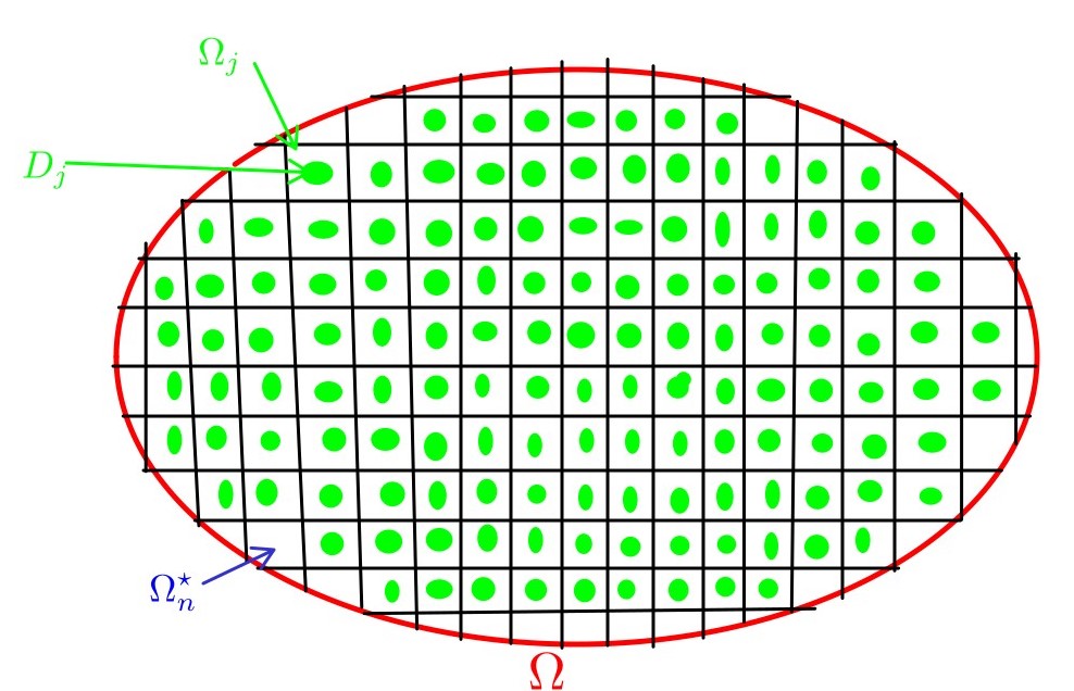
Figure 1. An illustration, in two-dimensional space, of $\Omega$ cutting using a schematic representation.

We rearrange the splitting of the domain $\Omega$ as $\Omega=\Omega_{cube}\cup\Omega_{r}$, with

$$\Omega_{cube}=\overset{M}{\underset{j=1}{\cup}}\Omega_{j}\;\;\text{and}\;\;\Omega_{r}=\underset{j-1}{\overset{\aleph}{\cup}}\Omega_{j}^{\star},\;\;\;\;M=M(a),\;\aleph=\aleph(a)\in\mathbb{N},$$

where $\Omega_{j}$’s are cubes located strictly within the interior of the domain $\Omega$. Each $\Omega_{j}$ contains one $D_{j}$ while the $\Omega_{j}^{\star}$’s do not contain any, see Figure 1. We observe that $\Omega_{cube}\subsetneq\Omega$.

Based on the introduced notations, in particular as $|\Omega_{j}|=a^{1-h}$, we can rewrite $(\ref{NewL.S.E})$ as

(4.22) $$Y(z_{m})-\sum_{j=1\atop j\neq m}^{M}G(z_{m};z_{j})\,\overline{\alpha}\,a^{1-h}\,Y(z_{j})=S(z_{m})+\overline{\alpha}\,\bm{\tilde{I}},$$

where

$$\bm{\tilde{I}}:=\int_{\Omega}G(z_{m};y)\,Y(y)\,dy-\,\sum_{j=1\atop j\neq m}^{M}G(z_{m};z_{j})\,Y(z_{j})\,\left|\Omega_{j}\right|.$$

To estimate $\bm{\tilde{I}}$, we first consider the term

$$\int_{\Omega}G(z_{m};y)\,Y(y)\,dy:=\int_{\Omega_{cube}}G(z_{m};y)\,Y(y)\,dy+\int_{\Omega_{r}}G(z_{m};y)\,Y(y)\,dy$$

and show that the second term is negligible. Indeed, regarding the domains $\Omega_{j}^{\star}$, which are not necessarily cubes, they have the no empty intersection property with $\partial\Omega$, i.e. $\partial\Omega_{n}^{\star}\cap\partial\Omega\neq\{\emptyset\}$, for $1\leq n\leq\aleph$. Since each $\Omega_{j}$ has volume equals to $a^{1-h}$, and then its maximum radius is of order $a^{\frac{1}{3}(1-h)}$ then intersecting surfaces with $\partial\Omega$ has volume of order $a^{\frac{2}{3}(1-h)}$. As the volume of $\partial\Omega$ is of order one, we conclude that the number of such cubes will not exceed the order $a^{-\frac{2}{3}(1-h)}$. Hence, the volume of $\Omega_{r}$ will not exceed the order $a^{\frac{1}{3}(1-h)}\underset{a\rightarrow 0}{\rightarrow}0$, i.e.

(4.23) $$\left|\Omega_{r}\right|=\mathcal{O}\left(a^{\frac{1}{3}(1-h)}\right).$$

Observe, due to Lemma 4.4, that we have

$$\left|\int_{\Omega_{r}}G(z_{m};y)\,Y(y)\,dy\right|\leq\|Y\|_{\mathbb{L}^{2}(\Omega_{r})}\left\|G(z_{m};\cdot)\right\|_{\mathbb{L}^{2}(\Omega_{r})}\leq\|Y\|_{\mathbb{L}^{2}(\Omega)}\;\left|\Omega_{r}\right|^{\frac{1-\delta}{3-\delta}}\;\left\|G(z_{m};\cdot)\right\|^{2}_{\mathbb{L}^{3-\delta}(\Omega_{r})},$$

and using the fact that $G(z_{m};\cdot)\in\mathbb{L}^{3-\delta}(\Omega_{r})$, hence $\left\|G(z_{m};\cdot)\right\|^{2}_{\mathbb{L}^{3-\delta}(\Omega_{r})}\sim 1$, we reduce the previous estimation to

(4.24) $$\left|\int_{\Omega_{r}}G(z_{m};y)\,Y(y)\,dy\right|\lesssim\|Y\|_{\mathbb{L}^{2}(\Omega)}\;\left|\Omega_{r}\right|^{\frac{1-\delta}{3-\delta}}\overset{(\ref{VolOmegar})}{\underset{(\ref{Yfctg})}{=}}\mathcal{O}\left(\left\|g\right\|_{\mathbb{H}^{-\frac{1}{2}}(\partial\Omega)}\;a^{\frac{(1-h)\,(1-\delta)}{3(3-\delta)}}\right),$$

which tends to zero with $a$. Therefore,

(4.25) $$\bm{\tilde{I}}=\bm{I}+\mathcal{O}\left(\left\|g\right\|_{\mathbb{H}^{-\frac{1}{2}}(\partial\Omega)}\;a^{\frac{(1-h)\,(1-\delta)}{3(3-\delta)}}\right),\quad\text{as}\quad a\ll 1,$$

where

(4.26) $$\bm{I}:=\sum_{\ell=1}^{M}\int_{\Omega_{\ell}}G(z_{m};y)\,Y(y)\,dy-\sum_{j=1\atop j\neq m}^{M}G(z_{m};z_{j})\,Y(z_{j})\,\left|\Omega_{j}\right|.$$

Let us now estimate $\bm{I}$. We write

$$\bm{I} = \sum_{\ell=1\atop\ell\neq m}^{M}\int_{\Omega_{\ell}}\left[G(z_{m};y)Y(y)-G(z_{m};z_{\ell})Y(z_{\ell})\right]\,dy+\int_{\Omega_{m}}G(z_{m};y)\,Y(y)\,dy,$$

and, by using Taylor expansion for the function $G(z_{m},\cdot)\,Y(\cdot)$ near the point $z_{\ell}$, we get:

$$\bm{I} = \sum_{\ell=1\atop\ell\neq m}^{M}\int_{\Omega_{\ell}}\int_{0}^{1}G(z_{m};z_{\ell}+t(y-z_{\ell}))\nabla Y\left(z_{\ell}+t(y-z_{\ell}\right)\cdot(y-z_{\ell})\,dt\,dy$$

$$+ \sum_{\ell=1\atop\ell\neq m}^{M}\int_{\Omega_{\ell}}\int_{0}^{1}Y\left(z_{\ell}+t(y-z_{\ell})\right)\nabla G(z_{m};z_{\ell}+t(y-z_{\ell}))\cdot(y-z_{\ell})dtdy+\int_{\Omega_{m}}G(z_{m};y)Y(y)dy.$$

From Lemma 4.2, we know that $G(x,y)=\phi(x,y)+\mathcal{R}(x,y)$, for $x\neq y$, where the dominant part $\phi(\cdot,\cdot)$ has a singularity at most of order 1, i.e. $\phi(x,y)\sim\frac{1}{\left|x-y\right|}$, for $x\neq y$, see Remark 6.1. In the sequel, we keep only the dominant part of $G(\cdot,\cdot)$. More precisely, we have

(4.27) $$\left|G(x,y)\right|\lesssim\frac{1}{\left|x-y\right|}\quad\text{and}\quad\left|\nabla G(x,y)\right|\lesssim\frac{1}{\left|x-y\right|^{2}},\quad\text{for}\quad x\neq y.$$

By taking the modulus in both sides and using $(\ref{SG})$, we deduce:

$$\left|\bm{I}\right| \lesssim a^{\frac{(1-h)}{3}}\sum_{\ell=1\atop\ell\neq m}^{M}\int_{\Omega_{\ell}}\int_{0}^{1}\frac{1}{\left|z_{m}-z_{\ell}-t(y-z_{\ell})\right|}\left|\nabla Y\left(z_{\ell}+t(y-z_{\ell}\right)\right|dt\,dy$$

$$+ a^{\frac{(1-h)}{3}}\sum_{\ell=1\atop\ell\neq m}^{M}\int_{\Omega_{\ell}}\int_{0}^{1}\frac{\left|Y\left(z_{\ell}+t(y-z_{\ell})\right)\right|}{\left|z_{m}-z_{\ell}-t(y-z_{\ell})\right|^{2}}\,dt\,dy+\int_{\Omega_{m}}\left|G(z_{m};y)\,\right|\left|Y(y)\,\right|dy.$$

Using the fact that $\left|\Omega_{\ell}\right|\sim a^{1-h}$, with $1\leq\ell\leq M$, we obtain:

$$\left|\bm{I}\right|\lesssim a^{\frac{5(1-h)}{6}}\sum_{\ell=1\atop\ell\neq m}^{M}\frac{\left\|\nabla Y\right\|_{\mathbb{L}^{2}(\Omega_{\ell})}}{\left|z_{m}-z_{\ell}\right|}+a^{\frac{5(1-h)}{6}}\sum_{\ell=1\atop\ell\neq m}^{M}\frac{\left\|Y\right\|_{\mathbb{L}^{2}(\Omega_{\ell})}}{\left|z_{m}-z_{\ell}\right|^{2}}+\left\|Y\,\right\|_{\mathbb{L}^{2}(\Omega_{m})}\;\left\|G(z_{m};\cdot)\right\|_{\mathbb{L}^{2}(\Omega_{m})}.$$

By making the use of Cauchy-Schwartz inequality we get

$$\left|\bm{I}\right| \lesssim a^{\frac{5(1-h)}{6}}\;\left\|\nabla Y\right\|_{\mathbb{L}^{2}(\Omega)}\;\left(\sum_{\ell=1\atop\ell\neq m}^{M}\frac{1}{\left|z_{m}-z_{\ell}\right|^{2}}\right)^{\frac{1}{2}}+a^{\frac{5(1-h)}{6}}\;\left\|Y\right\|_{\mathbb{L}^{2}(\Omega)}\;\left(\sum_{\ell=1\atop\ell\neq m}^{M}\frac{1}{\left|z_{m}-z_{\ell}\right|^{4}}\right)^{\frac{1}{2}}$$

$$+ \left\|Y\right\|_{\mathbb{L}^{2}(\Omega)}\;\left(\int_{\Omega_{m}}\frac{1}{\left|z_{m}-y\,\right|^{2}}\,dy\right)^{\frac{1}{2}}.$$

To comupte the sums appearing on the R.H.S, we use the fact that

(4.28) $$\sum_{j=1\atop j\neq m}^{M}\left|z_{i}-z_{j}\right|^{-k}=\begin{cases}\mathcal{O}\left(d^{-3}\right),&\text{for $k<3$}\\ \mathcal{O}\left(d^{-k}\right),&\text{for $k>3$}\end{cases},$$

see [3, Section 3.3] for more details. Hence,

(4.29) $$\left|\bm{I}\right|\lesssim a^{\frac{5(1-h)}{6}}\;\left\|\nabla Y\right\|_{\mathbb{L}^{2}(\Omega)}\;d^{-\frac{3}{2}}+a^{\frac{5(1-h)}{6}}\;\left\|Y\right\|_{\mathbb{L}^{2}(\Omega)}\;d^{-2}+\left\|Y\right\|_{\mathbb{L}^{2}(\Omega)}\;\left(\int_{\Omega_{m}}\frac{1}{\left|z_{m}-y\right|^{2}}dy\right)^{\frac{1}{2}}.$$

To achieve the estimation of $\bm{I}$, we set and we estimate the third term appearing on the R.H.S

$$\bm{I_{3}}=\int_{B(z_{m};r)}\frac{1}{\left|z_{m}-y\right|^{2}}\,dy+\int_{\Omega_{m}\setminus B(z_{m};r)}\frac{1}{\left|z_{m}-y\right|^{2}}\,dy,$$

where $B(z_{m};r)$ is the ball of center $z_{m}$ and radius $r$, where $r$ is such that $r\in\bm{I_{4}}:=\left[0;\frac{\sqrt{3}}{2}\,a^{\frac{(1-h)}{3}}\right]$. Then,

$$\bm{I_{3}} \lesssim \int_{0}^{r}\int_{\partial\,B(z_{m};s)}\frac{1}{\left|z_{m}-y\right|^{2}}\,d\sigma(y)\,ds+\frac{1}{r^{2}}\;\left|\Omega_{m}\setminus B(z_{m};r)\right|$$

$$= \int_{0}^{r}\,\frac{1}{s^{2}}\,\left|\partial\,B(z_{m};s)\right|\,ds+\frac{1}{r^{2}}\;\left|\Omega_{m}\setminus B(z_{m};r)\right|=\frac{8\,\pi\,r}{3}+\frac{1}{r^{2}}\;a^{1-h}\leq\;\underset{r\in\bm{I_{4}}}{\max}\,\rho(r,a),$$

where

$$\rho(r,a):=\frac{8\,\pi}{3}\,r+\frac{1}{r^{2}}\;a^{1-h}.$$

We have $\underset{r\in\bm{I_{4}}}{\max}\,\rho(r,a)=\rho(r_{sol},a)$, where $r_{sol}$ is such that $\partial_{r}\rho(r_{sol},a)=0$. Straightforward computations, gives us $r_{sol}=\left(\frac{3}{4\,\pi}\,a^{1-h}\right)^{\frac{1}{3}}$. Consequently,

$$\underset{r\in\bm{I_{4}}}{\max}\,\rho(r,a)=\left(48\,\pi^{2}\right)^{\frac{1}{3}}\,a^{\frac{(1-h)}{3}}.$$

Hence,

(4.30) $$\bm{I_{3}}=\mathcal{O}\left(a^{\frac{(1-h)}{3}}\right).$$

Finally, by gathering $(\ref{EstimationAI3})$ and $(\ref{AI3RHS})$ and using the fact that $d\sim a^{\frac{1-h}{3}}$, we end up with

$$\bm{I}\lesssim a^{\frac{(1-h)}{3}}\;\left\|\nabla Y\right\|_{\mathbb{L}^{2}(\Omega)}+a^{\frac{(1-h)}{6}}\;\left\|Y\right\|_{\mathbb{L}^{2}(\Omega)}\overset{(\ref{Yfctg})}{\lesssim}a^{\frac{(1-h)}{6}}\;\left\|g\right\|_{\mathbb{H}^{-\frac{1}{2}}(\partial\Omega)}.$$

Hence, using $(\ref{tildeI=I+err})$, we get

(4.31) $$\bm{\tilde{I}}=\mathcal{O}\left(a^{\frac{(1-\delta)\,(1-h)}{3(3-\delta)}}\;\left\|g\right\|_{\mathbb{H}^{-\frac{1}{2}}(\partial\Omega)}\right).$$

Finally, by going back to $(\ref{LSE=RHS+AI+AII})$ and making use of the estimation $(\ref{EstimationAI})$, we obtain

(4.32) $$Y(z_{m})-\alpha\,\sum_{j=1\atop j\neq m}^{M}G(z_{m};z_{j})\,Y(z_{j})=S(z_{m})+\mathcal{O}\left(\overline{\alpha}\,a^{\frac{(1-\delta)(1-h)}{3(3-\delta)}}\;\left\|g\right\|_{\mathbb{H}^{-\frac{1}{2}}(\partial\Omega)}\right).$$

Taking the difference between $(\ref{1924})$ and $(\ref{1918})$ gives us the following algebraic system:

$$\left(Y_{m}-Y(z_{m})\right)-\sum_{j=1\atop j\neq m}^{M}G(z_{m};z_{j})\;\overline{\alpha}\,a^{1-h}\,\left(Y_{j}-Y(z_{j})\right)=\mathcal{O}\left(\overline{\alpha}\,a^{\frac{(1-\delta)(1-h)}{3(3-\delta)}}\;\left\|g\right\|_{\mathbb{H}^{-\frac{1}{2}}(\partial\Omega)}\right).$$

Consequently,

$$\left|Y_{m}-Y(z_{m})\right|=\mathcal{O}\left(\overline{\alpha}\,a^{\frac{(1-\delta)(1-h)}{3(3-\delta)}}\;\left\|g\right\|_{\mathbb{H}^{-\frac{1}{2}}(\partial\Omega)}\right),\quad m=1,\cdots,M.$$

In particular

(4.33) $$\underset{1\leq m\leq M}{\max}\left|Y_{m}-Y(z_{m})\right|=\mathcal{O}\left(\overline{\alpha}\,a^{\frac{(1-h)(1-\delta)}{3(3-\delta)}}\;\left\|g\right\|_{\mathbb{H}^{-\frac{1}{2}}(\partial\Omega)}\right).$$

The previous estimation confirm the convergence of the discrete algebraic system to the continuous L.S.E.

4.4. Finishing the proof of Theorem 1.1

Now, we set $\bm{J}$ to be:

(4.34) $$\bm{J}:=\omega^{2}\,\frac{\rho_{1}}{k_{1}}\,\langle v^{g};p^{f}\rangle_{\mathbb{L}^{2}(D)}+P^{2}\,\langle u^{g};p^{f}\rangle_{\mathbb{L}^{2}(\Omega)}=\sum_{j=1}^{M}\left[\omega^{2}\,\frac{\rho_{1}}{k_{1}}\,\langle v^{g}_{j};p^{f}\rangle_{\mathbb{L}^{2}(D_{j})}+P^{2}\,\langle u^{g}_{j};p^{f}\rangle_{\mathbb{L}^{2}(\Omega_{j})}\right].$$

Then, by using the Taylor expansion for the function $p^{f}(\cdot)$ near the centres, we get:

(4.35) $$\bm{J}=\sum_{j=1}^{M}p^{f}(z_{j})\,\left[\omega^{2}\,\frac{\rho_{1}}{k_{1}}\,\int_{D_{j}}v^{g}_{j}(x)\,dx+P^{2}\,\int_{\Omega_{j}}u^{g}_{j}(x)\,dx\right]+\bm{Err_{J}},$$

where

$$\bm{Err_{J}} := \omega^{2}\,\frac{\rho_{1}}{k_{1}}\,\sum_{j=1}^{M}\int_{D_{j}}v^{g}_{j}(x)\,\int_{0}^{1}(x-z_{j})\cdot\nabla p^{f}(z_{j}+t(x-z_{j}))\,dt\,dx$$

$$+ P^{2}\,\sum_{j=1}^{M}\int_{\Omega_{j}}u^{g}_{j}(x)\,\int_{0}^{1}(x-z_{j})\cdot\nabla p^{f}(z_{j}+t(x-z_{j}))\,dt\,dx,$$

which can be estimated, by recalling that $\rho_{1}\sim 1;\,k_{1}\sim a^{2}$ and $\left|\Omega_{j}\right|\sim a^{1-h}$, as

$$\left|\bm{Err_{J}}\right| \lesssim a^{-1}\,\sum_{j=1}^{M}\left\|v^{g}_{j}\right\|_{\mathbb{L}^{2}(D_{j})}\,\left\|\nabla p^{f}\right\|_{\mathbb{L}^{2}(D_{j})}+a^{\frac{(1-h)}{3}}\,P^{2}\,\sum_{j=1}^{M}\left\|u^{g}_{j}\right\|_{\mathbb{L}^{2}(\Omega_{j})}\,\left\|\nabla p^{f}\right\|_{\mathbb{L}^{2}(\Omega_{j})}$$

$$\lesssim a^{-1}\,\left\|v^{g}\right\|_{\mathbb{L}^{2}(D)}\,\left\|\nabla p^{f}\right\|_{\mathbb{L}^{2}(D)}+a^{\frac{(1-h)}{3}}\,P^{2}\,\left\|u^{g}\right\|_{\mathbb{L}^{2}(\Omega)}\,\left\|\nabla p^{f}\right\|_{\mathbb{L}^{2}(\Omega)}$$

$$\overset{(\ref{Add-proof-1})}{\lesssim} a^{\frac{1}{2}}\,\left\|v^{g}\right\|_{\mathbb{L}^{2}(D)}\,\left\|f\right\|_{\mathbb{H}^{-\frac{1}{2}}(\partial\Omega)}+a^{\frac{(1-h)}{3}}\,P^{2}\,\left\|u^{g}\right\|_{\mathbb{L}^{2}(\Omega)}\,\left\|\nabla p^{f}\right\|_{\mathbb{L}^{2}(\Omega)}.$$

Next, we estimate $\left\|\nabla p^{f}\right\|_{\mathbb{L}^{2}(\Omega)}$. To do this, we recall from $(\ref{ETVKT})$ that

$$\nabla p^{f}(x)=\langle\nabla G(x,\cdot);f\rangle_{\mathbb{H}^{\frac{1}{2}}(\partial\Omega)\times\mathbb{H}^{-\frac{1}{2}}(\partial\Omega)}.$$

Then,

$$\left\|\nabla p^{f}\,\right\|_{\mathbb{L}^{2}(\Omega)}\leq\left\|f\right\|_{\mathbb{H}^{-\frac{1}{2}}(\partial\Omega)}\;\left[\int_{\Omega}\left\|\nabla G(x,\cdot)\right\|^{2}_{\mathbb{H}^{\frac{1}{2}}(\partial\Omega)}\,dx\right]^{\frac{1}{2}}=\mathcal{O}\left(\left\|f\right\|_{\mathbb{H}^{-\frac{1}{2}}(\partial\Omega)}\right).$$

Then, by using $(\ref{AprioriEstvf})$, we have

$$\left|\bm{Err_{J}}\right|\lesssim\left\|f\right\|_{\mathbb{H}^{-\frac{1}{2}}(\partial\Omega)}\,\left[\left\|g\right\|_{\mathbb{H}^{-\frac{1}{2}}(\partial\Omega)}\,a^{2-h}+a^{\frac{(1-h)}{3}}\,P^{2}\,\left\|u^{g}\right\|_{\mathbb{L}^{2}(\Omega)}\right].$$

The following lemma is needed to finish with the estimation of $\bm{Err_{J}}$.

Lemma 4.6.

The function $u^{g}(\cdot)$, solution of $(\ref{EquaWf})$, satisfies

$$\left\|u^{g}\right\|_{\mathbb{L}^{2}(\Omega)}\lesssim\frac{1}{P}\;\left\|g\right\|_{\mathbb{H}^{-\frac{1}{2}}\left(\partial\Omega\right)}.$$

Proof.

See Subsection 6.4. ∎

Then,

$$\left|\bm{Err_{J}}\right|\lesssim a^{\frac{(1-h)}{3}}\,P\,\left\|g\right\|_{\mathbb{H}^{-\frac{1}{2}}(\partial\Omega)}\,\left\|f\right\|_{\mathbb{H}^{-\frac{1}{2}}(\partial\Omega)}.$$

Going back to $(\ref{Equa0729})$, we obtain

$$\bm{J}=\sum_{j=1}^{M}p^{f}(z_{j})\,\left[\omega^{2}\,\frac{\rho_{1}}{k_{1}}\,\int_{D_{j}}v^{g}_{j}(x)\,dx+P^{2}\,\int_{\Omega_{j}}u^{g}_{j}(x)\,dx\right]+\mathcal{O}\left(a^{\frac{(1-h)}{3}}\,P\,\left\|f\right\|_{\mathbb{H}^{-\frac{1}{2}}(\partial\Omega)}\,\left\|g\right\|_{\mathbb{H}^{-\frac{1}{2}}(\partial\Omega)}\right).$$

Remark that $u^{g}(\cdot)$ is solution of the L.S.E given by $(\ref{NewL.S.E})$, i.e. $u^{g}(\cdot)=Y(\cdot)$, in $\Omega$. Using this, we obtain

$$\int_{\Omega_{j}}u^{g}_{j}(x)\,dx=\int_{\Omega_{j}}Y(x)\,dx=Y(z_{j})\,\left|\Omega_{j}\right|+\int_{\Omega_{j}}\int_{0}^{1}(x-z_{j})\cdot\nabla Y(z_{j}+t(x-z_{j}))\,dt\,dx.$$

Then,

(4.36) $$\bm{J} = \sum_{j=1}^{M}p^{f}(z_{j})\,\left[\omega^{2}\,\frac{\rho_{1}}{k_{1}}\,\int_{D_{j}}v^{f}_{j}(x)\,dx+P^{2}\,Y(z_{j})\,\left|\Omega_{j}\right|\right]$$

$$+ \sum_{j=1}^{M}p^{f}(z_{j})\,\left[P^{2}\,\int_{\Omega_{j}}\int_{0}^{1}(x-z_{j})\cdot\nabla Y(z_{j}+t(x-z_{j}))\,dt\,dx\right]$$

$$+ \mathcal{O}\left(a^{\frac{(1-h)}{3}}\,P\,\left\|f\right\|_{\mathbb{H}^{-\frac{1}{2}}(\partial\Omega)}\,\left\|g\right\|_{\mathbb{H}^{-\frac{1}{2}}(\partial\Omega)}\right).$$

We estimate the second term on the R.H.S, as

(4.37) $$\left|\cdots\right| \lesssim P^{2}\sum_{j=1}^{M}\left|p^{f}(z_{j})\right|\,\left|\int_{\Omega_{j}}\int_{0}^{1}(x-z_{j})\cdot\nabla Y(z_{j}+t(x-z_{j}))\,dt\,dx\right|$$

$$\leq P^{2}\,\left(\sum_{j=1}^{M}\left|p^{f}(z_{j})\right|^{2}\right)^{\frac{1}{2}}\,\left(\sum_{j=1}^{M}\left|\int_{\Omega_{j}}\int_{0}^{1}(x-z_{j})\cdot\nabla Y(z_{j}+t(x-z_{j}))\,dt\,dx\right|^{2}\right)^{\frac{1}{2}}$$

$$= \mathcal{O}\left(P^{2}\,\left(\sum_{j=1}^{M}\left|p^{f}(z_{j})\right|^{2}\right)^{\frac{1}{2}}\,a^{\frac{5}{6}(1-h)}\,\left\|\nabla Y\right\|_{\mathbb{L}^{2}(\Omega)}\right).$$

At this stage, we need first to estimate $\overset{M}{\underset{j=1}{\sum}}\left|p^{f}(z_{j})\right|^{2}$. To achieve this, we recall that $p^{f}(\cdot)$ is solution of $(\ref{EquaKg-introdution})$ and we set $\tilde{p}^{f}(\cdot)$ to be solution of

(4.38) $$\begin{cases}\Delta\,\tilde{p}^{f}=0\quad\text{in}\quad\Omega,\\ \partial_{\nu}\tilde{p}^{f}=f\;\;\;\text{on}\quad\partial\Omega.\end{cases}$$

Now, by subtracting $(\ref{EquaKg-introdution})$ from $(\ref{Equatildepf})$, we get

$$\begin{cases}\left(\Delta+\omega^{2}\,n^{2}\right)\,\left(p^{f}-\tilde{p}^{f}\right)=-\,\omega^{2}\,n^{2}\,\tilde{p}^{f}\quad\text{in}\quad\Omega,\\ \qquad\qquad\;\;\partial_{\nu}\left(p^{f}-\tilde{p}^{f}\right)=0\;\;\;\text{on}\quad\partial\Omega.\end{cases}$$

Its solution takes the following form

$$\left(p^{f}-\tilde{p}^{f}\right)(z)=\omega^{2}\;\int_{\Omega}G(z,y)\,n^{2}(y)\,\tilde{p}^{f}(y)\,dy,\quad z\in\Omega.$$

By taking the modulus we get

(4.39) $$\left|\left(p^{f}-\tilde{p}^{f}\right)(z)\right|\leq\omega^{2}\;\left\|n^{2}\right\|_{\mathbb{L}^{\infty}(\Omega)}\;\left\|G(z,\cdot)\right\|_{\mathbb{L}^{2}(\Omega)}\;\left\|\tilde{p}^{f}\right\|_{\mathbb{L}^{2}(\Omega)}\lesssim\left\|\tilde{p}^{f}\right\|_{\mathbb{L}^{2}(\Omega)},$$

where the last estimation is a consequence of the $\mathbb{L}^{2}(\Omega)$-integrability of the Green’s kernel $G(z,\cdot)$, uniformly on $z\in\Omega$, and the boundedness of $\omega^{2}\;\left\|n^{2}\right\|_{\mathbb{L}^{\infty}(\Omega)}$. In addition, we use the fact that $(\ref{Equatildepf})$ is a well posed problem to derive

(4.40) $$\left\|\tilde{p}^{f}\right\|_{\mathbb{L}^{2}(\Omega)}\lesssim\left\|f\right\|_{\mathbb{H}^{-\frac{1}{2}}(\partial\Omega)}.$$

Then, by gathering $(\ref{pf-tildepf})$ and $(\ref{WPP})$, we obtain:

(4.41) $$\left|\left(p^{f}-\tilde{p}^{f}\right)(z)\right|\lesssim\left\|f\right\|_{\mathbb{H}^{-\frac{1}{2}}(\partial\Omega)}.$$

For $\tilde{p}^{f}(\cdot)$ using its harmonicity in $\Omega$, we deduce that

$$\tilde{p}^{f}(z_{j})=\frac{1}{\left|\mathcal{B}_{j}\right|}\;\int_{\mathcal{B}_{j}}\tilde{p}^{f}(x)\;dx,$$

where $\mathcal{B}_{j}$ is the largest ball centred at $z_{j}$ and contained in the cube $\Omega_{j}$. We observe that, for $1\leq j\leq M$, we have $\left|\mathcal{B}_{j}\right|=\left|\mathcal{B}_{j_{0}}\right|\sim a^{1-h}\sim M^{-1}$. Then, using Hölder inequality, we deduce that:

(4.42) $$\left|\tilde{p}^{f}(z_{j})\right|\leq\left|\mathcal{B}_{j}\right|^{-\frac{1}{2}}\;\left\|\tilde{p}^{f}\right\|_{\mathbb{L}^{2}(\mathcal{B}_{j})}.$$

Therefore,

$$\sum_{j=1}^{M}\left|p^{f}(z_{j})\right|^{2}=\sum_{j=1}^{M}\left|\tilde{p}^{f}(z_{j})+\left(p^{f}(z_{j})-\tilde{p}^{f}(z_{j})\right)\right|^{2}\lesssim\sum_{j=1}^{M}\left|\tilde{p}^{f}(z_{j})\right|^{2}+\sum_{j=1}^{M}\left|p^{f}(z_{j})-\tilde{p}^{f}(z_{j})\right|^{2}.$$

By making the use of $(\ref{LAM})$ and $(\ref{MMTT})$, we obtain:

$$\sum_{j=1}^{M}\left|p^{f}(z_{j})\right|^{2} \lesssim \sum_{j=1}^{M}\left|\mathcal{B}_{j}\right|^{-1}\;\left\|\tilde{p}^{f}\right\|^{2}_{\mathbb{L}^{2}(\mathcal{B}_{j})}+M\;\left\|f\right\|^{2}_{\mathbb{H}^{-\frac{1}{2}}(\partial\Omega)}$$

$$\lesssim \left|\mathcal{B}_{j_{0}}\right|^{-1}\;\left\|\tilde{p}^{f}\right\|^{2}_{\mathbb{L}^{2}(\overset{M}{\underset{j=1}{\cup}}\mathcal{B}_{j})}+M\;\left\|f\right\|^{2}_{\mathbb{H}^{-\frac{1}{2}}(\partial\Omega)}.$$

As $\left|\mathcal{B}_{j_{0}}\right|_{-1}\sim M$ and $\overset{M}{\underset{j=1}{\cup}}\mathcal{B}_{j}\subset\Omega$, we obtain:

(4.43) $$\sum_{j=1}^{M}\left|p^{f}(z_{j})\right|^{2}\lesssim M\;\left(\left\|\tilde{p}^{f}\right\|^{2}_{\mathbb{L}^{2}(\Omega)}+\left\|f\right\|^{2}_{\mathbb{H}^{-\frac{1}{2}}(\partial\Omega)}\right)\overset{(\ref{WPP})}{\lesssim}M\;\left\|f\right\|^{2}_{\mathbb{H}^{-\frac{1}{2}}(\partial\Omega)}.$$

We continue with our estimation of $(\ref{0539})$ , using $(\ref{PfMf})$,

$$\left|\cdots\right|\lesssim P^{2}\,M^{\frac{1}{2}}\,\left\|f\right\|_{\mathbb{H}^{-\frac{1}{2}}(\partial\Omega)}\,a^{\frac{5}{6}(1-h)}\,\left\|\nabla Y\right\|_{\mathbb{L}^{2}(\Omega)}\overset{(\ref{Yfctg})}{=}\mathcal{O}\left(P^{2}\,a^{\frac{(1-h)}{3}}\,\left\|f\right\|_{\mathbb{H}^{-\frac{1}{2}}(\partial\Omega)}\,\left\|g\right\|_{\mathbb{H}^{-\frac{1}{2}}(\partial\Omega)}\right).$$

Then, $\bm{J}$ becomes

$$\bm{J}=\sum_{j=1}^{M}p^{f}(z_{j})\,\left[\omega^{2}\,\frac{\rho_{1}}{k_{1}}\,\int_{D_{j}}v^{g}_{j}(x)\,dx+P^{2}\,Y(z_{j})\,\left|\Omega_{j}\right|\right]+\mathcal{O}\left(a^{\frac{(1-h)}{3}}\,P^{2}\,\left\|f\right\|_{\mathbb{H}^{-\frac{1}{2}}(\partial\Omega)}\,\left\|g\right\|_{\mathbb{H}^{-\frac{1}{2}}(\partial\Omega)}\right).$$

To see how the parameter $P^{2}$ is related to the scattering coefficient $\alpha$, we set the following lemma.

Lemma 4.7.

The scattering coefficient $\alpha$, given by $(\ref{Defalpha})$, admits the following estimation:

(4.44) $$\alpha=-\;P^{2}\;a^{1-h}+\mathcal{O}\left(a\right),$$

where $0<h<1$, and

$$P^{2}:=\frac{-\,k_{0}\;\left(\langle 1;\overline{e}_{n_{0}}\rangle_{\mathbb{L}^{2}(B)}\right)^{2}}{\lambda_{n_{0}}^{B}\;c_{n_{0}}}\sim 1,$$

with respect to the parameter $a$.

Proof.

See Subsection 6.5. ∎

Knowing that $\left|\Omega_{j}\right|=a^{1-h}$ and using $(\ref{EstimationRealpha})$, we deduce that $P^{2}\,Y(z_{j})\,\left|\Omega_{j}\right|=-\,\alpha\,Y(z_{j})$. In addition, from $(\ref{DefYj})$, we have

$$\omega^{2}\,\frac{\rho_{1}}{k_{1}}\,\int_{D_{j}}v_{j}^{g}(x)\;dx=\alpha\,Y_{j}.$$

Hence, we end up with the coming formula

$$\bm{J}=\sum_{j=1}^{M}p^{f}(z_{j})\,\alpha\,\left[Y_{j}-Y(z_{j})\right]+\mathcal{O}\left(a^{\frac{(1-h)}{3}}\,P^{2}\,\left\|f\right\|_{\mathbb{H}^{-\frac{1}{2}}(\partial\Omega)}\,\left\|g\right\|_{\mathbb{H}^{-\frac{1}{2}}(\partial\Omega)}\right).$$

By taking the modulus in both sides of the previous inequality, we get:

$$\left|\bm{J}\right| \lesssim \left|\alpha\right|\,M^{\frac{1}{2}}\,\underset{1\leq j\leq M}{\max}\left|Y_{j}-Y(z_{j})\right|\;\left(\sum_{j=1}^{M}\left|p^{f}(z_{j})\right|^{2}\right)^{\frac{1}{2}}+a^{\frac{(1-h)}{3}}\,P^{2}\,\left\|f\right\|_{\mathbb{H}^{-\frac{1}{2}}(\partial\Omega)}\,\left\|g\right\|_{\mathbb{H}^{-\frac{1}{2}}(\partial\Omega)}$$

$$\overset{(\ref{PfMf})}{\lesssim} \left|\alpha\right|\,M\,\underset{1\leq j\leq M}{\max}\left|Y_{j}-Y(z_{j})\right|\;\left\|f\right\|_{\mathbb{H}^{-\frac{1}{2}}(\partial\Omega)}+a^{\frac{(1-h)}{3}}\,P^{2}\,\left\|f\right\|_{\mathbb{H}^{-\frac{1}{2}}(\partial\Omega)}\,\left\|g\right\|_{\mathbb{H}^{-\frac{1}{2}}(\partial\Omega)}.$$

Noticing that $M\sim a^{h-1}$, using the fact that $\alpha\sim P^{2}\,a^{1-h}$, see $(\ref{EstimationRealpha})$ and taking into account the estimation derived in $(\ref{maxY-Y})$, we obtain:

$$\left|\bm{J}\right| \lesssim a^{\frac{(1-h)(1-\delta)}{3(3-\delta)}}\,P^{2}\,\left\|f\right\|_{\mathbb{H}^{-\frac{1}{2}}(\partial\Omega)}\,\left\|g\right\|_{\mathbb{H}^{-\frac{1}{2}}(\partial\Omega)}+a^{\frac{(1-h)}{3}}\,P^{2}\,\left\|f\right\|_{\mathbb{H}^{-\frac{1}{2}}(\partial\Omega)}\,\left\|g\right\|_{\mathbb{H}^{-\frac{1}{2}}(\partial\Omega)}$$

$$= \mathcal{O}\left(a^{\frac{(1-h)(1-\delta)}{3(3-\delta)}}\,P^{2}\,\left\|f\right\|_{\mathbb{H}^{-\frac{1}{2}}(\partial\Omega)}\,\left\|g\right\|_{\mathbb{H}^{-\frac{1}{2}}(\partial\Omega)}\right).$$

Now, by gathering $(\ref{Lambda-d--Lambda-P})$ and $(\ref{DefJ})$, we obtain:

$$\left|\langle\left(\Lambda_{D}-\Lambda_{P}\right)(f);g\rangle_{\mathbb{H}^{\frac{1}{2}}(\partial\Omega)\times\mathbb{H}^{-\frac{1}{2}}(\partial\Omega)}\right|\lesssim a^{\frac{(1-h)(1-\delta)}{3(3-\delta)}}\,P^{2}\,\left\|f\right\|_{\mathbb{H}^{-\frac{1}{2}}(\partial\Omega)}\,\left\|g\right\|_{\mathbb{H}^{-\frac{1}{2}}(\partial\Omega)}.$$

This suggest,

$$\left\|\Lambda_{D}-\Lambda_{P}\right\|_{\mathcal{L}(\mathbb{H}^{-\frac{1}{2}}(\partial\Omega);\mathbb{H}^{\frac{1}{2}}(\partial\Omega))}\lesssim a^{\frac{(1-h)(1-\delta)}{3(3-\delta)}}\,P^{2}.$$

This proves $(\ref{energy-D})$ and ends the proof of Theorem 1.1.

5. Proof of Lemma 4.3

This section is divided into two subsections. In the first one we show that the continuous integral equation is invertible, by transforming the satisfied PDE into an integral equation involving positive operators. In the second subsection we relate the algebraic system that we desire to invert, see $(\ref{Equa1138})$, to the continuously invertible integral equation.

5.1. Invertibility of the continuous integral equations

We observe that $u^{g}(\cdot)$, solution of $(\ref{EquaWf})$, can be represented as a solution of the following integral equation

(5.1) $$u^{g}+N^{\phi}_{\Omega}\left(\bm{\alpha}\,u^{g}\right)=\tilde{g},$$

where $N^{\phi}_{\Omega}$ is the Newtonian operator defined by $(\ref{DefNPO})$ and $\bm{\alpha}(\cdot):=\left(P^{2}-\omega^{2}\,n^{2}(\cdot)\right)$. Observe that, as $P^{2}\gg 1$, we have $\bm{\alpha}(\cdot)>0$. After multiplying both sides of the previous equation with $\bm{\alpha}$, we obtain

(5.2) $$\bm{\alpha}\,u^{g}+\bm{\alpha}\,N^{\phi}_{\Omega}\left(\bm{\alpha}\,u^{g}\right)=\bm{\alpha}\,\tilde{g}.$$

Next, we set $\gimel_{1}(\cdot;\cdot)$ to be the bilinear form defined by

$$\gimel_{1}(u;v):=\langle\bm{\alpha}\,u;v\rangle_{\mathbb{L}^{2}(\Omega)}+\langle\bm{\alpha}\,N^{\phi}_{\Omega}\left(\bm{\alpha}\,u\right);v\rangle_{\mathbb{L}^{2}(\Omega)},$$

and, we set $\gimel_{2}(\cdot)$ to be the linear form defined by

$$\gimel_{2}(v):=\langle\bm{\alpha}\,\tilde{g};v\rangle_{\mathbb{L}^{2}(\Omega)}.$$

It is clear that $\gimel_{2}(\cdot)$ is a continuous linear form. For $\gimel_{1}(\cdot,\cdot)$, using the continuity of the Newtonian operator, we can prove that $\gimel_{1}(\cdot,\cdot)$ is a continuous bilinear form. In addition, from the positivity of the Newtonian operator, we have

$$\langle u;\bm{\alpha}\,N^{\phi}_{\Omega}\left(\bm{\alpha}\,u\right)\rangle_{\mathbb{L}^{2}(\Omega)}\geq c_{0}\;\left(\underset{\Omega}{\min}\left|\bm{\alpha}\right|\right)^{2}\;\left\|u\right\|^{2}_{\mathbb{L}^{2}(\Omega)},$$

where $c_{0}$ is the positivity constant of the Newtonian operator. This allows us to obtain:

$$\gimel_{1}(u,u)\geq\underset{\Omega}{\min}\left|\bm{\alpha}\right|\;\left(1+c_{0}\;\underset{\Omega}{\min}\left|\bm{\alpha}\right|\right)\;\left\|u\right\|^{2}_{\mathbb{L}^{2}(\Omega)},$$

which proves the coercivity of $\gimel_{1}(\cdot,\cdot)$. Thanks to Lax-Milgram theorem, see [5, Corollary 5.8], we deduce the existence and uniqueness of the solution to $(\ref{InjIE})$, in $\mathbb{L}^{2}(\Omega)$. In other words, the integral equation given by $(\ref{WIE})$ is invertible. Moreover the function $u^{g}(\cdot)$, solution of $(\ref{WIE})$, admits the following estimation:

(5.3) $$\left\|u^{g}\right\|_{\mathbb{L}^{2}(\Omega)}\leq\frac{\left\|\bm{\alpha}\right\|_{\mathbb{L}^{\infty}(\Omega)}}{\underset{\Omega}{\min}\left|\bm{\alpha}\right|\;\left(1+c_{0}\;\underset{\Omega}{\min}\left|\bm{\alpha}\right|\right)}\;\left\|\tilde{g}\right\|_{\mathbb{L}^{2}(\Omega)}\lesssim\frac{1}{P^{2}}\;\left\|\tilde{g}\right\|_{\mathbb{L}^{2}(\Omega)}.$$

5.2. Relating the algebraic system to the continuous integral equation

From $(\ref{0820})$, we have

(5.4) $$Y_{m}-\sum_{j\neq m}G(z_{m};z_{j})\;\overline{\alpha}\,a^{1-h}Y_{j}=S(z_{m})+\dfrac{\omega^{2}\,\rho_{1}}{k_{1}\,\alpha}\;Rest_{m}.$$

where $Y_{m}$ is defined by $(\ref{DefYj})$ and $Rest_{m}$ is given by $(\ref{DefRestm})$. We have seen that $\alpha=-\,P^{2}\,a^{1-h}+\mathcal{O}\left(a\right)$, see $(\ref{EstimationRealpha})$. Then, by keeping its dominant part and using the fact that $\left|\Omega_{j}\right|=a^{1-h}$, for $1\leq j\leq M$, we deduce that $\alpha$ can be approximated by $\alpha=-\,P^{2}\,\left|\Omega_{j}\right|$. Hence, we rewrite the previous equation as

$$Y_{m}\;+\;\sum_{j=1\atop j\neq m}^{M}G(z_{m};z_{j})\;P^{2}\,\left|\Omega_{j}\right|\;Y_{j}\; = S(z_{m})+\dfrac{\omega^{2}\,\rho_{1}}{k_{1}\,\alpha}\;Rest_{m}$$

$$Y_{m}\;+\;P^{2}\;\sum_{j=1\atop j\neq m}^{M}\int_{\Omega}G(z_{m};z_{j})\,{\mathchoice{\raisebox{0.0pt}{$\displaystyle\chi$}}{\raisebox{0.0pt}{$\textstyle\chi$}}{\raisebox{0.0pt}{$\scriptstyle\chi$}}{\raisebox{0.0pt}{$\scriptscriptstyle\chi$}}}_{\Omega_{j}}(x)\;Y_{j}\;dx = S(z_{m})+\dfrac{\omega^{2}\,\rho_{1}}{k_{1}\,\alpha}\;Rest_{m}.$$

Multiplying the two sides of the previous equation with ${\mathchoice{\raisebox{0.0pt}{$\displaystyle\chi$}}{\raisebox{0.0pt}{$\textstyle\chi$}}{\raisebox{0.0pt}{$\scriptstyle\chi$}}{\raisebox{0.0pt}{$\scriptscriptstyle\chi$}}}_{\Omega_{m}}(\cdot)$ and summing up with respect to the index $m$, we get:

$$\sum_{m=1}^{M}{\mathchoice{\raisebox{0.0pt}{$\displaystyle\chi$}}{\raisebox{0.0pt}{$\textstyle\chi$}}{\raisebox{0.0pt}{$\scriptstyle\chi$}}{\raisebox{0.0pt}{$\scriptscriptstyle\chi$}}}_{\Omega_{m}}(\cdot)Y_{m}\;+\;P^{2}\;\sum_{m=1}^{M}\,{\mathchoice{\raisebox{0.0pt}{$\displaystyle\chi$}}{\raisebox{0.0pt}{$\textstyle\chi$}}{\raisebox{0.0pt}{$\scriptstyle\chi$}}{\raisebox{0.0pt}{$\scriptscriptstyle\chi$}}}_{\Omega_{m}}(\cdot)\sum_{j=1\atop j\neq m}^{M}\int_{\Omega}G(z_{m};z_{j})\,{\mathchoice{\raisebox{0.0pt}{$\displaystyle\chi$}}{\raisebox{0.0pt}{$\textstyle\chi$}}{\raisebox{0.0pt}{$\scriptstyle\chi$}}{\raisebox{0.0pt}{$\scriptscriptstyle\chi$}}}_{\Omega_{j}}(x)\;Y_{j}\;dx = \sum_{m=1}^{M}\,{\mathchoice{\raisebox{0.0pt}{$\displaystyle\chi$}}{\raisebox{0.0pt}{$\textstyle\chi$}}{\raisebox{0.0pt}{$\scriptstyle\chi$}}{\raisebox{0.0pt}{$\scriptscriptstyle\chi$}}}_{\Omega_{m}}(\cdot)S(z_{m})$$

$$+ \dfrac{\omega^{2}\,\rho_{1}}{k_{1}\,\alpha}\;\sum_{m=1}^{M}{\mathchoice{\raisebox{0.0pt}{$\displaystyle\chi$}}{\raisebox{0.0pt}{$\textstyle\chi$}}{\raisebox{0.0pt}{$\scriptstyle\chi$}}{\raisebox{0.0pt}{$\scriptscriptstyle\chi$}}}_{\Omega_{m}}(\cdot)Rest_{m}.$$

which can be rewritten using the notations

(5.5) $$\bm{Y}(\cdot):=\sum_{m=1}^{M}{\mathchoice{\raisebox{0.0pt}{$\displaystyle\chi$}}{\raisebox{0.0pt}{$\textstyle\chi$}}{\raisebox{0.0pt}{$\scriptstyle\chi$}}{\raisebox{0.0pt}{$\scriptscriptstyle\chi$}}}_{\Omega_{m}}(\cdot)Y_{m}\;\;\text{and}\;\;\bm{S}(\cdot):=\sum_{m=1}^{M}{\mathchoice{\raisebox{0.0pt}{$\displaystyle\chi$}}{\raisebox{0.0pt}{$\textstyle\chi$}}{\raisebox{0.0pt}{$\scriptstyle\chi$}}{\raisebox{0.0pt}{$\scriptscriptstyle\chi$}}}_{\Omega_{m}}(\cdot)S(z_{m})\;\;\text{and}\;\;\bm{R}(\cdot):=\sum_{m=1}^{M}{\mathchoice{\raisebox{0.0pt}{$\displaystyle\chi$}}{\raisebox{0.0pt}{$\textstyle\chi$}}{\raisebox{0.0pt}{$\scriptstyle\chi$}}{\raisebox{0.0pt}{$\scriptscriptstyle\chi$}}}_{\Omega_{m}}(\cdot)Rest_{m},$$

as

(5.6) $$\bm{Y}(\cdot)\;+\;P^{2}\;\sum_{m=1}^{M}\,{\mathchoice{\raisebox{0.0pt}{$\displaystyle\chi$}}{\raisebox{0.0pt}{$\textstyle\chi$}}{\raisebox{0.0pt}{$\scriptstyle\chi$}}{\raisebox{0.0pt}{$\scriptscriptstyle\chi$}}}_{\Omega_{m}}(\cdot)\sum_{j=1\atop j\neq m}^{M}\int_{\Omega}G(z_{m};z_{j})\,{\mathchoice{\raisebox{0.0pt}{$\displaystyle\chi$}}{\raisebox{0.0pt}{$\textstyle\chi$}}{\raisebox{0.0pt}{$\scriptstyle\chi$}}{\raisebox{0.0pt}{$\scriptscriptstyle\chi$}}}_{\Omega_{j}}(x)\;Y_{j}\;dx=\bm{S}(\cdot)+\dfrac{\omega^{2}\,\rho_{1}}{k_{1}\,\alpha}\;\bm{R}(\cdot).$$

The goal of the next lemma is to prove that the second term on the L.H.S converges, in $\mathbb{L}^{1}(\Omega)$, to a function which belongs to the range of the Newtonian operator.

Lemma 5.1.

We have the following estimation

(5.7) $$\left\|N\left(\bm{Y}\right)(\cdot)-\sum_{m=1}^{M}\,{\mathchoice{\raisebox{0.0pt}{$\displaystyle\chi$}}{\raisebox{0.0pt}{$\textstyle\chi$}}{\raisebox{0.0pt}{$\scriptstyle\chi$}}{\raisebox{0.0pt}{$\scriptscriptstyle\chi$}}}_{\Omega_{m}}(\cdot)\sum_{j=1\atop j\neq m}^{M}\int_{\Omega}G(z_{m};z_{j})\,{\mathchoice{\raisebox{0.0pt}{$\displaystyle\chi$}}{\raisebox{0.0pt}{$\textstyle\chi$}}{\raisebox{0.0pt}{$\scriptstyle\chi$}}{\raisebox{0.0pt}{$\scriptscriptstyle\chi$}}}_{\Omega_{j}}(x)\;Y_{j}\;dx\right\|_{\mathbb{L}^{1}(\Omega)}\lesssim a^{\frac{1}{6}(1-h)}\,\left\|\bm{Y}\right\|_{\mathbb{L}^{2}(\Omega)},$$

where $N$ is the Newtonian operator defined by

$$N(f)(x):=\int_{\Omega}G(x,y)\,f(y)\,dy.$$

Proof.

See Subsection 6.6. ∎

Thanks to the previous lemma, we rewrite $(\ref{DHB})$ as

(5.8) $$\left(I\;+\;P^{2}\,N\right)\,\left(\bm{Y}\right)(\cdot)=\bm{S}(\cdot)+\bm{r}(\cdot),$$

where

$$\bm{r}(\cdot):=\dfrac{\omega^{2}\,\rho_{1}}{k_{1}\,\alpha}\;\bm{R}(\cdot)+P^{2}\,\left[N\left(\bm{Y}\right)(\cdot)-\sum_{m=1}^{M}\,{\mathchoice{\raisebox{0.0pt}{$\displaystyle\chi$}}{\raisebox{0.0pt}{$\textstyle\chi$}}{\raisebox{0.0pt}{$\scriptstyle\chi$}}{\raisebox{0.0pt}{$\scriptscriptstyle\chi$}}}_{\Omega_{m}}(\cdot)\sum_{j=1\atop j\neq m}^{M}\int_{\Omega}G(z_{m};z_{j})\,{\mathchoice{\raisebox{0.0pt}{$\displaystyle\chi$}}{\raisebox{0.0pt}{$\textstyle\chi$}}{\raisebox{0.0pt}{$\scriptstyle\chi$}}{\raisebox{0.0pt}{$\scriptscriptstyle\chi$}}}_{\Omega_{j}}(x)\;Y_{j}\;dx\right],$$

with

(5.9) $$\left\|\bm{r}\right\|_{\mathbb{L}^{2}(\Omega)}=\mathcal{O}\left(a^{\frac{(1-h)}{6}}\,P^{2}\,\left\|\bm{Y}\right\|_{\mathbb{L}^{2}(\Omega)}\right).$$

We can check that $\bm{Y}(\cdot)$ is solution of $(\ref{EquaWf})$, with source term given by $\bm{S}(\cdot)+\bm{r}(\cdot)$. We have proved in Subsection 5.1 the existence and uniqueness of solution of $(\ref{EquaWf})$, which is equivalent to the invertibility of $(\ref{IEI})$, i.e. $\bm{Y}(\cdot)$ exist. In addition, thanks to $(\ref{Ss51})$, the solution $\bm{Y}(\cdot)$ satisfies

$$\left\|\bm{Y}\right\|_{\mathbb{L}^{2}(\Omega)}\lesssim\frac{1}{P^{2}}\;\left\|\bm{S}+\bm{r}\right\|_{\mathbb{L}^{2}(\Omega)}\overset{(\ref{estimationr})}{\lesssim}\frac{1}{P^{2}}\;\left\|\bm{S}\right\|_{\mathbb{L}^{2}(\Omega)}+a^{\frac{1}{6}(1-h)}\;\left\|\bm{Y}\right\|_{\mathbb{L}^{2}(\Omega)}.$$

Hence, as $h<1$ and $a\ll 1$, we deduce that

$$\left\|\bm{Y}\right\|_{\mathbb{L}^{2}(\Omega)}\lesssim\frac{1}{P^{2}}\;\left\|\bm{S}\right\|_{\mathbb{L}^{2}(\Omega)}.$$

This implies the injectivity of $(\ref{IEI})$. In addition, it is known that any injective linear map between two finite dimensional vector spaces of the same dimension is surjective. This proves the surjectivity and, consequently, the bijectivity of $(\ref{IEI})$. Hence, we have also the invertibility of the algebraic system $(\ref{ASEqua1})$. In addition, as by construction,

$$\|\bm{Y}\|^{2}_{\mathbb{L}^{2}(\Omega)}=\sum_{m=1}^{M}|Y_{m}|^{2}|\Omega_{m}|=\left|\Omega_{m_{0}}\right|\;\sum_{m=1}^{M}\left|Y_{m}\right|^{2},$$

similarly for $\bm{S}$, with the $\Omega_{m}$’s having equivalent volumes, we deduce the estimate

$$\left(\sum_{m=1}^{M}\left|Y_{m}\right|^{2}\right)^{\frac{1}{2}}\lesssim\frac{1}{P^{2}}\;\left(\sum_{m=1}^{M}\left|S(z_{m})\right|^{2}\right)^{\frac{1}{2}}.$$

This concludes the proof of Lemma 4.3.

6. Appendix

This section is organised as follows. We start by proving Lemma 2.1 related to the smallness of the Newtonian operator $N^{p}$ with respect to the parameter $P$. Next, it is important to first examine the proof of Lemma 4.2, on the analysis of the Green’s kernel decomposition $G(\cdot;\cdot)=\phi(\cdot;\cdot)+\mathcal{R}(\cdot;\cdot)$, before moving on to the proof of Lemma 4.1, giving us an a priori estimation satisfied by the acoustic field $v^{g}(\cdot)$. Then, we continue with the proof of Lemma 4.6. Later, we examine the proof of Lemma 4.7, which gives us an estimation of the scattering coefficient $\alpha$. Finally, we conclude this section by proving Lemma 5.1.

6.1. Proof of Lemma 2.1

From the spectral theory, we have

$$\left\|N^{p}\right\|_{\mathcal{L}\left(\mathbb{L}^{2}(\Omega);\mathbb{L}^{2}(\Omega)\right)}=\left\|\mathcal{R}(P^{2};\Delta)\right\|_{\mathcal{L}\left(\mathbb{L}^{2}(\Omega);\mathbb{L}^{2}(\Omega)\right)}\leq\frac{1}{\mathrm{dist}\left(P^{2};\sigma(\Delta)\right)},$$

where $\sigma(\Delta)$ stands for the spectrum of the Laplacian operator in $\mathbb{L}^{2}(\Omega)$. It is known that $\sigma(\Delta):=\left\{\mu_{n}\right\}_{n\geq 1}$ such that $0>\mu_{1}>\mu_{2}>\mu_{3}>\cdots\rightarrow-\infty$. Hence, we get $\mathrm{dist}\left(P^{2};\sigma(\Delta)\right)>P^{2}$. Consequently,

$$\left\|N^{p}\right\|_{\mathcal{L}\left(\mathbb{L}^{2}(\Omega);\mathbb{L}^{2}(\Omega)\right)}\leq\frac{1}{P^{2}}.$$

This proves $(\ref{NormNewtonian})$. To prove $(\ref{TraceNormNewtonian})$, we start by remarking that for an arbitrary function $f\in\mathbb{L}^{2}(\Omega)$, the function $N^{p}(f)$ satisfies the problem

$$\begin{cases}\left(\Delta-P^{2}\,I\right)N^{p}(f)=-\,f\quad\text{in}\quad\Omega,\\ \qquad\quad\quad\partial_{\nu}N^{p}(f)=\quad 0\;\;\;\,\text{on}\quad\partial\Omega.\end{cases}$$

Multiplying both sides of the first equation by $N^{p}(f)$ and integrating in $\Omega$, we get

$$\left\|\nabla N^{p}(f)\right\|^{2}_{\mathbb{L}^{2}(\Omega)} \leq P^{2}\,\left\|N^{p}(f)\right\|^{2}_{\mathbb{L}^{2}(\Omega)}+\left\|f\right\|_{\mathbb{L}^{2}(\Omega)}\;\left\|N^{p}(f)\right\|_{\mathbb{L}^{2}(\Omega)}$$

$$\leq P^{2}\,\left\|N^{p}\right\|^{2}_{\mathcal{L}\left(\mathbb{L}^{2}(\Omega);\mathbb{L}^{2}(\Omega)\right)}\,\left\|f\right\|^{2}_{\mathbb{L}^{2}(\Omega)}+\left\|f\right\|^{2}_{\mathbb{L}^{2}(\Omega)}\;\left\|N^{p}\right\|_{\mathcal{L}\left(\mathbb{L}^{2}(\Omega);\mathbb{L}^{2}(\Omega)\right)}.$$

Hence,

(6.1) $$\left\|\nabla N^{p}\right\|^{2}_{\mathcal{L}\left(\mathbb{L}^{2}(\Omega);\mathbb{L}^{2}(\Omega)\right)}\leq P^{2}\,\left\|N^{p}\right\|^{2}_{\mathcal{L}\left(\mathbb{L}^{2}(\Omega);\mathbb{L}^{2}(\Omega)\right)}+\left\|N^{p}\right\|_{\mathcal{L}\left(\mathbb{L}^{2}(\Omega);\mathbb{L}^{2}(\Omega)\right)}\overset{(\ref{NormNewtonian})}{=}\mathcal{O}\left(\frac{1}{P^{2}}\right).$$

Then,

$$\left\|N^{p}\right\|_{\mathcal{L}\left(\mathbb{L}^{2}(\Omega);\mathbb{H}^{1}(\Omega)\right)}:=\left[\left\|N^{p}\right\|^{2}_{\mathcal{L}\left(\mathbb{L}^{2}(\Omega);\mathbb{L}^{2}(\Omega)\right)}+\left\|\nabla N^{p}\right\|^{2}_{\mathcal{L}\left(\mathbb{L}^{2}(\Omega);\mathbb{L}^{2}(\Omega)\right)}\right]^{\frac{1}{2}},$$

which, using $(\ref{NormNewtonian})$ and $(\ref{EstimationnablaN})$, becomes $\left\|N^{p}\right\|_{\mathcal{L}\left(\mathbb{L}^{2}(\Omega);\mathbb{H}^{1}(\Omega)\right)}=\mathcal{O}\left(\dfrac{1}{P}\right)$ and, by taking the trace operator we end up with the following estimation

$$\left\|\gamma N^{p}\right\|_{\mathcal{L}\left(\mathbb{L}^{2}(\Omega);\mathbb{H}^{\frac{1}{2}}(\partial\Omega)\right)}=\mathcal{O}\left(\frac{1}{P}\right).$$

This proves $(\ref{TraceNormNewtonian})$ and ends the proof of Lemma 2.1.

6.2. Proof of Lemma 4.2

We split our proof into two steps. The first one consists in estimating the singularity of the dominant part of $G(\cdot,\cdot)$, and in the second one we deal with the remainder term.

1. Estimation of the scale of $\phi$.
   We recall that $\phi$ is solution of

   $$\begin{cases}\Delta\phi=-\,\delta\quad\text{in}\quad\Omega_{a},\\ \partial_{\nu}\phi=\;\;0\quad\text{on}\quad\partial\Omega_{a},\end{cases}$$

   where $\Omega_{a}:=z+a\,\Omega_{1}$, and $\Omega_{1}$ is bounded connected domain such that $\left|\Omega_{1}\right|\sim 1$. Now, let $f$ be an arbitrary function, then

   (6.2) $$u(x):=\int_{\Omega_{a}}\phi(x,y)f(y)\,dy,$$

   is a solution of

   $$\begin{cases}-\Delta u=f\quad\text{in}\quad\Omega_{1},\\ \partial_{\nu}u=0\;\;\quad\text{on}\quad\partial\Omega_{1}.\end{cases}$$

   By scaling the previous PDE, we get:

   (6.3) $$\begin{cases}-\Delta\tilde{u}=a^{2}\,\tilde{f}\quad\text{in}\quad\Omega,\\ \partial_{\nu}\tilde{u}=0\quad\text{on}\quad\partial\Omega.\end{cases}$$

   Moreover, by scaling the integral solution representation, see $(\ref{IRS})$, we obtain:

   (6.4) $$\tilde{u}(x)=a^{3}\;\int_{\Omega_{1}}\tilde{\phi}(x,y)\tilde{f}(y)\,dy.$$

   In addition, the integral equation solution of the scaled PDE, see $(\ref{ScaledPDE})$, is

   (6.5) $$\tilde{u}(x)=a^{2}\;\int_{\Omega_{1}}\phi^{\star}(x,y)\tilde{f}(y)\,dy,$$

   where $\phi^{\star}$ is solution of

   $$\begin{cases}\Delta\phi^{\star}=-\,\delta\quad\text{in}\quad\Omega_{1},\\ \partial_{\nu}\phi^{\star}=\;\;0\quad\text{on}\quad\partial\Omega_{1}.\end{cases}$$

   By gathering $(\ref{IRSscaled})$ and $(\ref{IRSscaledPDE})$, we deduce

   $$a^{3}\;\int_{\Omega_{1}}\tilde{\phi}(x,y)\tilde{f}(y)\,dy=a^{2}\;\int_{\Omega_{1}}\phi^{\star}(x,y)\tilde{f}(y)\,dy,\qquad\forall\;\;f.$$

   This implies the following scale

   (6.6) $$\tilde{\phi}(\cdot,\cdot)=a^{-1}\;\phi^{\star}(\cdot,\cdot).$$

   Remark 6.1.

   In the singularity analysis point of view, we deduce, from $(\ref{SFS})$, that

   (6.7) $$\phi(x,y)\sim\frac{1}{\left|x-y\right|},\quad x\neq y.$$

2. Estimation of the remainder term.
   By multiplying both sides of $(\ref{RemainderPDE})$ by $\phi(\cdot,\cdot)$, solution of $(\ref{phi-harmonic})$, integrating by parts, using the fact that $\partial_{\nu}\mathcal{R}_{\big{|}_{\partial\Omega}}=\partial_{\nu}\phi_{\big{|}_{\partial\Omega}}=0$, $\Delta\phi=-\delta$, in $\Omega$, and multiplying by $n^{2}(\cdot)$, we obtain:

   (6.8) $$\left(I-\omega^{2}\;n^{2}(\cdot)\;N^{\phi}\right)\left(n^{2}\,\mathcal{R}(\cdot,y)\right)(x)=\omega^{2}\,n^{2}(x)\,\int_{\Omega}n^{2}(t)\,\phi(x,t)\,\phi(t,y)\,dt.$$

   Based on Remark 6.1, we have the following estimation on the R.H.S,

   $$\left|\omega^{2}\,n^{2}(x)\,\int_{\Omega}n^{2}(t)\,\phi(x,t)\,\phi(t,y)\,dt\right|\overset{(\ref{phisin})}{\lesssim}\int_{\Omega}\frac{1}{\left|t-x\right|}\,\frac{1}{\left|t-y\right|}\,dt\overset{(\star)}{\leq}c_{2}(\Omega)\,\left|x-y\right|+c_{2}(\Omega)=\mathcal{O}\left(1\right),$$

   where $(\star)$ is justified in [34, Lemma 4.1]. This implies that the term on the R.H.S of $(\ref{RIEII})$ is in $\mathbb{L}^{p}(\Omega),\;\forall\,p\in[1,+\infty]$. Knowing that, for any bounded domain $\Omega\subset\mathbb{R}^{3}$, the Newtonian operator $N^{\phi}$ is a bounded operator from $\mathbb{L}^{p}(\Omega)$ onto $\mathbb{W}^{2,p}(\Omega)$, see [14], we deduce that, for fixed $y\in\Omega$, the term $n^{2}(\cdot)\,\mathcal{R}(\cdot,y)$ is in $\mathbb{W}^{2,p}(\Omega),\;\forall\,p\in[1,+\infty]$. In particular, $\mathcal{R}(\cdot,y)\in\mathbb{L}^{\infty}(\Omega)$.

This concludes the proof of Lemma 4.2.

6.3. Proof of Lemma 4.1

We start by recalling, from $(\ref{L.S.E.vf})$, that $v^{g}(\cdot)$ is solution of:

(6.9) $$v^{g}(x)-\omega^{2}\,\frac{\rho_{1}}{k_{1}}\;\int_{D}G(x,y)\,v^{g}(y)\,dy=S(x),\quad x\in D.$$

In the sequel, we divide the proof into two steps.

2. The case of one droplet. Using the decomposition $(\ref{G=phi+Remainder})$, of the Green’s kernel $G(\cdot,\cdot)$, we rewrite $(\ref{L.S.E.vf.Lemma})$ as

   $$v^{g}(x)-\omega^{2}\,\frac{\rho_{1}}{k_{1}}\;\int_{D}\phi(x,y)\,v^{g}(y)\,dy=S(x)+\omega^{2}\,\frac{\rho_{1}}{k_{1}}\;\int_{D}\mathcal{R}(x,y)\,v^{g}(y)\,dy.$$

   Next, we denote by $\left(\lambda_{n};e_{n}\right)$ the eigensystem associated to the Newtonian operator $N_{D}^{\phi}$ in $\mathbb{L}^{2}(D)$. Then, after taking the inner product with respect to $e_{n}$ and the square modulus in both sides of the previous equation, we get

   $$\left|\langle v^{g};e_{n}\rangle\right|^{2} \leq \frac{2\,k_{1}^{2}}{\left|k_{1}-\omega^{2}\;\rho_{1}\,\lambda_{n}\right|^{2}}\,\left[\left|\langle S;e_{n}\rangle\right|^{2}+\left|\frac{\omega^{2}\,\rho_{1}}{k_{1}}\right|^{2}\,\left|\langle\int_{D}\mathcal{R}(\cdot,y)\,v^{g}(y)\,dy;e_{n}\rangle\right|^{2}\right].$$

   Then, by summing up with respect to the index $n$ and taking into account the relations $(\ref{DispersionEqua})$ and $(\ref{ScaleBulk})$ we obtain

   $$\left\|v^{g}\right\|^{2}_{\mathbb{L}^{2}(D)}\lesssim a^{-2h}\;\left[\left\|S\right\|^{2}_{\mathbb{L}^{2}(D)}+a^{-4}\,\left\|\int_{D}\mathcal{R}(\cdot,y)\,v^{g}(y)\,dy\right\|^{2}_{\mathbb{L}^{2}(D)}\right].$$

   We estimate the second term on the R.H.S, as

   $$\bm{R_{1}}:=\left\|\int_{D}\mathcal{R}(\cdot,y)\,v^{g}(y)\,dy\right\|^{2}_{\mathbb{L}^{2}(D)}\leq\int_{D}\int_{D}\left|\mathcal{R}(x,y)\right|^{2}\,dy\;dx\;\left\|v^{g}\right\|^{2}_{\mathbb{L}^{2}(D)}.$$

   From Lemma 4.2, we know that $\mathcal{R}(\cdot,y)\in\mathbb{L}^{\infty}(\Omega)$. Then, $\int_{D}\int_{D}\left|\mathcal{R}(x,y)\right|^{2}\,dy\;dx\lesssim a^{6},$ and,

   (6.10) $$\bm{R_{1}}:=\left\|\int_{D}\mathcal{R}(\cdot,y)\,v^{g}(y)\,dy\right\|^{2}_{\mathbb{L}^{2}(D)}\lesssim a^{6}\;\left\|v^{g}\right\|^{2}_{\mathbb{L}^{2}(D)}.$$

   Then,

   $$\left\|v^{g}\right\|^{2}_{\mathbb{L}^{2}(D)}\lesssim a^{-2h}\;\left\|S\right\|^{2}_{\mathbb{L}^{2}(D)}+a^{2-2\,h}\,\left\|v^{g}\right\|^{2}_{\mathbb{L}^{2}(D)},$$

   which becomes,

   $$\left\|v^{g}\right\|_{\mathbb{L}^{2}(D)}\lesssim a^{-h}\;\left\|S\right\|_{\mathbb{L}^{2}(D)}=\mathcal{O}\left(a^{\frac{3}{2}-h}\right).$$

4. The case of multiple droplets. From $(\ref{L.S.E.vf.Lemma})$, by taking $x\in D_{m}$, we get:

   $$v^{g}_{m}=\left(I-\frac{\omega^{2}\,\rho_{1}}{k_{1}}\;N_{D_{m}}^{\phi}\right)^{-1}\left[S_{m}+\frac{\omega^{2}\,\rho_{1}}{k_{1}}\;\sum_{j=1\atop j\neq m}^{M}\int_{D_{j}}G(\cdot,y)\,v^{g}_{j}(y)\,dy+\frac{\omega^{2}\,\rho_{1}}{k_{1}}\;\int_{D_{m}}\mathcal{R}(\cdot,y)\,v^{g}_{m}(y)\,dy\right].$$

   By taking the $\mathbb{L}^{2}(D_{m})$-norm, using $(\ref{Rvf})$ and

   $$\left\|\left(I-\dfrac{\omega^{2}\,\rho_{1}}{k_{1}}\;N_{D_{m}}^{\phi}\right)^{-1}\right\|_{\mathcal{L}(\mathbb{L}^{2}(D_{m});\mathbb{L}^{2}(D_{m}))}\lesssim a^{-h},$$

   proved for the case of one droplet, we get:

   $$\left\|v^{g}_{m}\right\|_{\mathbb{L}^{2}(D_{m})}\lesssim a^{-h}\;\left\|S_{m}\right\|_{\mathbb{L}^{2}(D_{m})}+a^{-2-h}\;\sum_{j=1\atop j\neq m}^{M}\left\|\int_{D_{j}}G(\cdot,y)\,v^{g}_{j}(y)\,dy\right\|_{\mathbb{L}^{2}(D_{m})}.$$

   We estimate the second term on the R.H.S.

   $$\bm{R_{2}} := \sum_{j=1\atop j\neq m}^{M}\left\|\int_{D_{j}}G(\cdot,y)\,v^{g}_{j}(y)\,dy\right\|_{\mathbb{L}^{2}(D_{m})}$$

   $$\overset{(\ref{SG})}{\lesssim} a^{3}\;\sum_{j=1\atop j\neq m}^{M}\frac{1}{\left|z_{m}-z_{j}\right|}\;\left\|v^{g}_{j}\right\|_{\mathbb{L}^{2}(D_{j})}\lesssim a^{3}\;\left[\sum_{j=1\atop j\neq m}^{M}\frac{1}{\left|z_{m}-z_{j}\right|^{2}}\right]^{\frac{1}{2}}\;\left\|v^{g}\right\|_{\mathbb{L}^{2}(D)}.$$

   Using $(\ref{SID})$ we reduce the previous estimation to:

   $$\bm{R_{2}}\lesssim a^{3}\;d^{-1}\;\left\|v^{g}\right\|_{\mathbb{L}^{2}(D)}=\mathcal{O}\left(a^{\frac{8+h}{3}}\;\left\|v^{g}\right\|_{\mathbb{L}^{2}(D)}\right).$$

   Then,

   $$\left\|v^{g}_{m}\right\|_{\mathbb{L}^{2}(D_{m})} \lesssim a^{-h}\;\left\|S_{m}\right\|_{\mathbb{L}^{2}(D_{m})}+a^{\frac{2-2h}{3}}\;\left\|v^{g}\right\|_{\mathbb{L}^{2}(D)}$$

   By taking the square, summing up with respect to the index $m$ and using the fact that $M\sim a^{h-1}$, we get, as $h<1$,

   $$\left\|v^{g}\right\|^{2}_{\mathbb{L}^{2}(D)} \lesssim a^{-2h}\;\left\|S\right\|^{2}_{\mathbb{L}^{2}(D)}+a^{\frac{(1-h)}{3}}\;\left\|v^{g}\right\|^{2}_{\mathbb{L}^{2}(D)}$$

   $$\left\|v^{g}\right\|^{2}_{\mathbb{L}^{2}(D)} \lesssim a^{-2h}\;\left\|S\right\|^{2}_{\mathbb{L}^{2}(D)}.$$

   Finally,

   (6.11) $$\left\|v^{g}\right\|_{\mathbb{L}^{2}(D)}\lesssim a^{-h}\;\left\|S\right\|_{\mathbb{L}^{2}(D)}=\mathcal{O}\left(a^{\frac{3}{2}-h}\right).$$

In addition, we can check, from $(\ref{EquaSg})$, that $S(\cdot)$ can be represented as a single layer with respect to the source data $g$, i.e. $S(\cdot)=SL(g)(\cdot)$. This implies, using the previous derived estimation,

$$\left\|v^{g}\right\|_{\mathbb{L}^{2}(D)}\lesssim a^{-h}\;\left\|SL(g)\right\|_{\mathbb{L}^{2}(D)}.$$

Next, we have

$$\left\|SL(g)\right\|_{\mathbb{L}^{2}(D)}:=\left[\int_{D}\left|\int_{\partial\Omega}G(x,y)\,g(y)\,dy\right|^{2}\;dx\right]^{\frac{1}{2}} = \left[\int_{D}\left|\langle G(x,\cdot);g\rangle_{\mathbb{H}^{\frac{1}{2}}(\partial\Omega)\times\mathbb{H}^{-\frac{1}{2}}(\partial\Omega)}\right|^{2}\;dx\right]^{\frac{1}{2}}$$

$$\leq \left\|g\right\|_{\mathbb{H}^{-\frac{1}{2}}(\partial\Omega)}\;\left[\int_{D}\left\|G(x,\cdot)\right\|^{2}_{\mathbb{H}^{\frac{1}{2}}(\partial\Omega)}\;dx\right]^{\frac{1}{2}}.$$

As the function inside the integral is smooth, we end up with the following estimation:

$$\left\|SL(g)\right\|_{\mathbb{L}^{2}(D)}\leq\left\|g\right\|_{\mathbb{H}^{-\frac{1}{2}}(\partial\Omega)}\;a^{\frac{3}{2}}.$$

The previous estimation combined with $(\ref{Equa1001})$ gives us

(6.12) $$\left\|v^{g}\right\|_{\mathbb{L}^{2}(D)}\lesssim a^{\frac{3}{2}-h}\;\left\|g\right\|_{\mathbb{H}^{-\frac{1}{2}}(\partial\Omega)}.$$

This ends the proof of Lemma 4.1.

6.4. Proof of Lemma 4.6

The function $u^{g}(\cdot)$, solution $(\ref{EquaWf})$, satisfies the following integral equation

$$u^{g}(x)=\omega^{2}\,N^{p}\left(n^{2}\,u^{g}\right)(x)+SL^{p}\left(g\right)(x),$$

where $SL^{p}$ is the Single-Layer operator. Then, by taking the $\mathbb{L}^{2}(\Omega)$-norm in both sides of the previous equation, we obtain:

$$\left\|u^{g}\right\|_{\mathbb{L}^{2}(\Omega)} \leq \omega^{2}\;\left\|N^{p}\right\|_{\mathcal{L}(\mathbb{L}^{2}(\Omega);\mathbb{L}^{2}(\Omega))}\;\left\|n^{2}\right\|_{\mathbb{L}^{\infty}(\Omega)}\;\left\|u^{g}\right\|_{\mathbb{L}^{2}(\Omega)}+\left\|SL^{p}\left(g\right)\right\|_{\mathbb{L}^{2}(\Omega)}$$

$$\left\|u^{g}\right\|_{\mathbb{L}^{2}(\Omega)} \overset{(\ref{CdtCvgS})}{\leq} \left\|SL^{p}\left(g\right)\right\|_{\mathbb{L}^{2}(\Omega)}.$$

Next, we estimate $\left\|SL^{p}\left(g\right)\right\|_{\mathbb{L}^{2}(\Omega)}$. To achieve this, straightforward computations give us,

$$\left\|SL^{p}\left(g\right)\right\|_{\mathbb{L}^{2}(\Omega)} \leq \left\|g\right\|_{\mathbb{H}^{-\frac{1}{2}}(\partial\Omega)}\;\left[\int_{\Omega}\left\|G_{p}(x,\cdot)\right\|^{2}_{\mathbb{H}^{\frac{1}{2}}(\partial\Omega)}dx\,\right]^{\frac{1}{2}}$$

$$\leq \left\|g\right\|_{\mathbb{H}^{-\frac{1}{2}}(\partial\Omega)}\;\left\|\gamma\,N^{p}\right\|_{\mathcal{L}\left(\mathbb{L}^{2}(\Omega);\mathbb{H}^{\frac{1}{2}}(\partial\Omega)\right)}\overset{(\ref{TraceNormNewtonian})}{=}\mathcal{O}\left(\frac{1}{P}\left\|g\right\|_{\mathbb{H}^{-\frac{1}{2}}(\partial\Omega)}\right).$$

Hence,

$$\left\|u^{g}\right\|_{\mathbb{L}^{2}(\Omega)}\lesssim\frac{1}{P}\;\left\|g\right\|_{\mathbb{H}^{-\frac{1}{2}}(\partial\Omega)}.$$

This concludes the proof of Lemma 4.6.

6.5. Proof of Lemma 4.7

We know that, for $m$ fixed,

$$\alpha:=\int_{D_{m}}W_{m}(x)\,dx=\int_{D_{m}}\left(\dfrac{k_{1}}{\omega^{2}\,\rho_{1}}\;I-N_{D_{m}}^{\phi}\right)^{-1}\left(1\right)(x)\;dx.$$

By expanding the constant function 1 over the basis of the Newtonian operator $N_{D_{m}}^{\phi}$ we obtain

(6.13) $$\alpha=\sum_{n}\;\langle 1;e_{n}\rangle_{\mathbb{L}^{2}(D_{m})}\;\int_{D_{m}}\left(\dfrac{k_{1}}{\omega^{2}\,\rho_{1}}\;I-N_{D_{m}}^{\phi}\right)^{-1}\left(e_{n}\right)(x)\;dx=\sum_{n}\;\left(\langle 1;e_{n}\rangle\right)^{2}\;\frac{\omega^{2}\,\rho_{1}}{\left(k_{1}-\omega^{2}\,\rho_{1}\,\lambda_{n}\right)}.$$

We chose $\omega^{2}$ such that

(6.14) $$\left|k_{1}-\omega^{2}\,\rho_{1}\,\lambda_{n}\right|=\begin{cases}a^{2+h},&\text{if $n=n_{0}$}\\ a^{2},&\text{otherwise}\end{cases}$$

Then,

$$\alpha=\left(\langle 1;e_{n_{0}}\rangle_{\mathbb{L}^{2}(D_{m})}\right)^{2}\;\;\frac{\omega^{2}\,\rho_{1}}{\left(k_{1}-\omega^{2}\,\rho_{1}\,\lambda_{n_{0}}\right)}+\sum_{n\neq n_{0}}\;\left(\langle 1;e_{n}\rangle_{\mathbb{L}^{2}(D_{m})}\right)^{2}\;\;\frac{\omega^{2}\,\rho_{1}}{\left(k_{1}-\omega^{2}\,\rho_{1}\,\lambda_{n}\right)}$$

We estimate the second term on the R.H.S as

$$\left|T_{R.H.S}\right|\lesssim\sum_{n\neq n_{0}}\frac{\left|\langle 1;e_{n}\rangle_{\mathbb{L}^{2}(D_{m})}\right|^{2}}{\left|k_{1}-\omega^{2}\,\rho_{1}\,\lambda_{n}\right|}\overset{(\ref{closeres})}{\lesssim}a^{-2}\;\left\|1\right\|^{2}_{\mathbb{L}^{2}(D_{m})}=\mathcal{O}\left(a\right).$$

Hence,

(6.15) $$\alpha=\left(\langle 1;e_{n_{0}}\rangle_{\mathbb{L}^{2}(D_{m})}\right)^{2}\;\frac{\omega^{2}\,\rho_{1}}{\left(k_{1}-\omega^{2}\;\rho_{1}\,\lambda_{n_{0}}\right)}+\mathcal{O}\left(a\right).$$

We chose $\omega$ solution of the coming dispersion equation

$$k_{1}-\omega^{2}\;\rho_{1}\,\lambda_{n_{0}}=c_{n_{0}}\,a^{2+h},\quad c_{n_{0}}\in\mathbb{R},\quad c_{n_{0}}\,\sim 1.$$

By solving the previous quadratic equation we obtain

$$\omega^{2}=\frac{k_{1}-c_{n_{0}}\;a^{2+h}}{\rho_{1}\,\lambda_{n_{0}}}.$$

And, by plugging the previous relation into $(\ref{alphabtreim})$, we obtain

$$\alpha=\frac{\left(k_{1}-c_{n_{0}}\;a^{2+h}\right)}{\lambda_{n_{0}}\;c_{n_{0}}\;a^{2+h}}\;\left(\langle 1;e_{n_{0}}\rangle_{\mathbb{L}^{2}(D_{m})}\right)^{2}+\mathcal{O}\left(a\right).$$

Knowing that $\langle 1;e_{n_{0}}\rangle_{\mathbb{L}^{2}(D_{m})}=a^{\frac{3}{2}}\,\langle 1;\overline{e}_{n_{0}}\rangle_{\mathbb{L}^{2}(B)}$ and using the fact that $k_{1}=a^{2}\,k_{0};\,\lambda_{n_{0}}=a^{2}\,\lambda_{n_{0}}^{B}$, we rewrite the previous equation like

$$\alpha=\frac{\left(k_{0}-c_{n_{0}}\;a^{h}\right)}{\lambda_{n_{0}}^{B}\;c_{n_{0}}}\;\left(\langle 1;\overline{e}_{n_{0}}\rangle_{\mathbb{L}^{2}(B)}\right)^{2}\;a^{1-h}+\mathcal{O}\left(a\right)=\frac{k_{0}}{\lambda_{n_{0}}^{B}\;c_{n_{0}}}\;\left(\langle 1;\overline{e}_{n_{0}}\rangle_{\mathbb{L}^{2}(B)}\right)^{2}\;a^{1-h}+\mathcal{O}\left(a\right).$$

We set $P^{2}$ to be the scaled dominant part of $\alpha$, i.e.

$$P^{2}:=\frac{-\,k_{0}\;\left(\langle 1;\overline{e}_{n_{0}}\rangle_{\mathbb{L}^{2}(B)}\right)^{2}}{\lambda_{n_{0}}^{B}\;c_{n_{0}}},$$

and we end up with the following formula

$$\alpha=-\,P^{2}\,a^{1-h}+\mathcal{O}\left(a\right).$$

This concludes the proof of Lemma 4.7.

6.6. Proof of Lemma 5.1

We compute the $\mathbb{L}^{1}(\Omega)$-norm of the difference between the R.H.S and the L.H.S appearing in $(\ref{LHSRHS})$,

$$\left\|\cdots\right\|_{\mathbb{L}^{1}(\Omega)}:=\int_{\Omega}\left|\int_{\Omega}G(y,x)\,\bm{Y}(x)\;dx-\sum_{m=1}^{M}\,{\mathchoice{\raisebox{0.0pt}{$\displaystyle\chi$}}{\raisebox{0.0pt}{$\textstyle\chi$}}{\raisebox{0.0pt}{$\scriptstyle\chi$}}{\raisebox{0.0pt}{$\scriptscriptstyle\chi$}}}_{\Omega_{m}}(y)\sum_{j=1\atop j\neq m}^{M}\int_{\Omega}G(z_{m};z_{j})\,{\mathchoice{\raisebox{0.0pt}{$\displaystyle\chi$}}{\raisebox{0.0pt}{$\textstyle\chi$}}{\raisebox{0.0pt}{$\scriptstyle\chi$}}{\raisebox{0.0pt}{$\scriptscriptstyle\chi$}}}_{\Omega_{j}}(x)\;Y_{j}\;dx\right|\,dy.$$

In contrary to Subsection 4.3, where the cutting of $\Omega$ onto $\underset{j=1}{\overset{M}{\cup}}\Omega_{j}$ and $\underset{j=1}{\overset{\aleph}{\cup}}\Omega_{j}^{\star}$ was of capital importance to derive the exact dominant term related to $\int_{\Omega_{j}}u^{g}(x)\,dx$, for $1\leq j\leq M$. Here, we need only to estimate functions (not to extract dominant term) defined in $\Omega$, thus involving both $\underset{j=1}{\overset{M}{\cup}}\Omega_{j}$ and $\underset{j=1}{\overset{\aleph}{\cup}}\Omega_{j}^{\star}$. Because, for every $1\leq j\leq M$ and $1\leq k\leq\aleph$, we have $\left|\Omega_{j}\right|\sim a^{1-h}\sim\left|\Omega_{k}^{\star}\right|$, we do not need to specify, in our comping computations, if we are dealing with $\left\{\Omega_{j}\right\}_{j=1}^{M}$ or $\left\{\Omega_{j}^{\star}\right\}_{j=1}^{\aleph}$. Moreover, to write short, we use the notation $\Omega_{j}$ for the domains $\Omega_{j}^{\star}$. Then,

$$\left\|\cdots\right\|_{\mathbb{L}^{1}(\Omega)} = \int_{\Omega}\left|\sum_{m=1}^{M}\,\left(\int_{\Omega}G(y,x)\,\bm{Y}(x)\;dx-\sum_{j=1\atop j\neq m}^{M}\int_{\Omega}G(z_{m};z_{j})\,{\mathchoice{\raisebox{0.0pt}{$\displaystyle\chi$}}{\raisebox{0.0pt}{$\textstyle\chi$}}{\raisebox{0.0pt}{$\scriptstyle\chi$}}{\raisebox{0.0pt}{$\scriptscriptstyle\chi$}}}_{\Omega_{j}}(x)\;Y_{j}\;dx\right){\mathchoice{\raisebox{0.0pt}{$\displaystyle\chi$}}{\raisebox{0.0pt}{$\textstyle\chi$}}{\raisebox{0.0pt}{$\scriptstyle\chi$}}{\raisebox{0.0pt}{$\scriptscriptstyle\chi$}}}_{\Omega_{m}}(y)\right|\,dy$$

$$= \sum_{m=1}^{M}\,\int_{\Omega_{m}}\left|\int_{\Omega}G(y,x)\,\bm{Y}(x)\;dx-\sum_{j=1\atop j\neq m}^{M}\int_{\Omega}G(z_{m};z_{j})\,{\mathchoice{\raisebox{0.0pt}{$\displaystyle\chi$}}{\raisebox{0.0pt}{$\textstyle\chi$}}{\raisebox{0.0pt}{$\scriptstyle\chi$}}{\raisebox{0.0pt}{$\scriptscriptstyle\chi$}}}_{\Omega_{j}}(x)\;Y_{j}\;dx\right|\,dy.$$

Using the definition of $\bm{Y}(\cdot)$, see $(\ref{DefYDefS})$, and the triangular inequality we rewrite the previous equation as

$$\left\|\cdots\right\|_{\mathbb{L}^{1}(\Omega)} \leq \sum_{m=1}^{M}\left|Y_{m}\right|\,\int_{\Omega_{m}}\int_{\Omega_{m}}\left|G(y,x)\right|\;dx\,dy$$

$$+ \sum_{m=1}^{M}\,\int_{\Omega_{m}}\left|\sum_{j=1\atop j\neq m}^{M}Y_{j}\;\int_{\Omega_{j}}\left(G(y,x)-G(z_{m};z_{j})\right)\;dx\right|\,dy.$$

Using Taylor expansion for the function $G(\cdot;\cdot)$, near the centres, we get

$$G(y,x)-G(z_{m};z_{j})=\int_{0}^{1}(x-z_{j})\cdot\nabla G(z_{m};z_{j}+t(x-z_{j}))\,dt+\int_{0}^{1}(y-z_{m})\cdot\nabla G(z_{m}+t(y-z_{m});x)\,dt.$$

We plug the previous expansion into the previous estimation, use $(\ref{SG})$ and the fact that $M\sim a^{h-1}$ to reduce the previous estimation to:

$$\left\|\cdots\right\|_{\mathbb{L}^{1}(\Omega)} \lesssim \underset{m}{\max}\int_{\Omega_{m}}\int_{\Omega_{m}}\frac{1}{\left|y-x\right|}\;dx\,dy\,\sum_{m=1}^{M}\left|Y_{m}\right|+\underset{j}{\max}\int_{\Omega_{j}}\left|x-z_{j}\right|\;dx\,\sum_{j=1\atop j\neq m}^{M}\left|Y_{j}\right|\;\frac{1}{\left|z_{j}-z_{m}\right|^{2}}$$

$$\lesssim \left|Y\right|\,M^{\frac{1}{2}}\,\underset{m}{\max}\int_{\Omega_{m}}\int_{\Omega_{m}}\frac{1}{\left|y-x\right|}\;dx\,dy+\underset{j}{\max}\int_{\Omega_{j}}\left|x-z_{j}\right|\;dx\,\left|Y\right|\,\left(\sum_{j=1\atop j\neq m}^{M}\frac{1}{\left|z_{j}-z_{m}\right|^{4}}\right)^{\frac{1}{2}}.$$

Moreover, we have the following estimations:

$$\underset{m}{\max}\int_{\Omega_{m}}\int_{\Omega_{m}}\frac{1}{\left|y-x\right|}\;dx\,dy=\mathcal{O}\left(a^{\frac{5}{3}(1-h)}\right)\;\,\text{and}\;\,\underset{j}{\max}\int_{\Omega_{j}}\left|x-z_{j}\right|\;dx=\mathcal{O}\left(a^{\frac{4}{3}(1-h)}\right).$$

Then,

$$\left\|\cdots\right\|_{\mathbb{L}^{1}(\Omega)}\lesssim\left|Y\right|\,\,a^{\frac{7}{6}(1-h)}+a^{\frac{4}{3}(1-h)}\,\left|Y\right|\,d^{-2}=\mathcal{O}\left(a^{\frac{2}{3}(1-h)}\,\left|Y\right|\right)\overset{(\ref{DefYDefS})}{=}\mathcal{O}\left(a^{\frac{1}{6}(1-h)}\,\left\|\bm{Y}\right\|_{\mathbb{L}^{2}(\Omega)}\right).$$

This concludes the proof of Lemma 5.1.

References

• [1] G. Alessandrini, Stable determination of conductivity by boundary measurements. Appl. Anal. 27 (1988), no. 1-3, 153-172.
• [2] G. Alessandrini, Singular solutions of elliptic equations and the determination of conductivity by boundary measurements. J. Differential Equations 84 (1990), no. 2, 252-272.
• [3] H. Ammari, D. P. Challa, A. P. Choudhury and M. Sini, The point-interaction approximation for the fields generated by contrasted bubbles at arbitrary fixed frequencies, Journal of Differential Equations, volume 267, number 4, pages 2104-2191, 2019.
• [4] R. Brown, Global uniqueness in the impedance-imaging problem for less regular conductivities SIAM J. Math. Anal., 27 (1996), pp. 1049-1056.
• [5] H. Brezis, Functional analysis, Sobolev spaces and partial differential equations, 2010, Springer Science & Business Media.
• [6] R. M. Brown, Global uniqueness in the impedance-imaging problem for less regular conductivities, SIAM Journal on Mathematical Analysis, volume 27, number 4, pages 1049-1056, 1996.
• [7] R. Brown, R. Torres Uniqueness in the inverse conductivity problem for conductivities with $3/2$ derivatives in $L^{p}$ , $p>2n$ J. Fourier Anal. Appl., 9 (2003), pp. 563-574.
• [8] R. M. Brown and G. Uhlmann, Uniqueness in the inverse conductivity problem for nonsmooth conductivities in two dimensions, Communications in Partial Differential Equations, volume 22, pages 1009-1027, 1997.
• [9] A. L. Bukhgeim, Recovering a potential from Cauchy data in the two-dimensional case, Walter de Gruyter, 2008.
• [10] D. P. Challa, A. Mantile and M. Sini, Characterization of the acoustic fields scattered by a cluster of small holes, Asymptotic Analysis, volume 118, number 4, pages 235–268, IOS Press, 2020.
• [11] S. Chanillo, A Problem in Electrical Prospection and a n-Dimensional Borg-Levinson Theorem, American Mathematical Society, number 3, pages 761–767, volume 108, 1990.
• [12] P. Caro and K. Rogers, Global uniqueness for the Calderón problem with Lipschitz conductivities. Forum Mathematics, Pi, volume 4, 2016.
• [13] P. Caro and A, Garcia, Scattering with critically-singular and $\delta$-shell potentials. Comm. Math. Phys. volume 379, no. 2, pages 543–587, 2020.
• [14] D. Colton and R. Kress, Inverse acoustic and electromagnetic scattering theory, 93, 2019, Springer Nature.
• [15] A. Dabrowski, A. Ghandriche and M. Sini, Mathematical analysis of the acoustic imaging modality using bubbles as contrast agents at nearly resonating frequencies, Inverse Problems and Imaging, vol. 15, num. 3, pages 555-597, 2021.
• [16] A. Ghandriche and M. Sini, Photo-acoustic inversion using plasmonic contrast agents: The full Maxwell model, Journal of Differential Equations, vol. 341, pages 1-78, 2022.
• [17] A. Ghandriche and M. Sini, Mathematical analysis of the photo-acoustic imaging modality using resonating dielectric nano-particles: The 2D TM-model, Journal of Mathematical Analysis and Applications, volume 506, number 2, pages 125658, Elsevier, 2022.
• [18] A. Ghandriche and M. Sini, Simultaneous Reconstruction of Optical and Acoustical Properties in Photo-Acoustic Imaging using plasmonics, arXiv, 2022.
• [19] B. Haberman and D. Tataru, Uniqueness in Calderón problem with Lipschitz conductivities Duke Math. J., 162 (2013), pp. 497-516.
• [20] B. Haberman, Uniqueness in Calderón’s problem for conductivities with unbounded gradient Comm. Math. Phys., 340 (2015), pp. 639-659.
• [21] V. Isakov, Completeness of products of solutions and some inverse problems for PDE, Journal of Differential Equations, Volume 92, Pages 305-316, 1991.
• [22] V. Isakov, Inverse Problems for Partial Differential Equations (second edition), Springer, New York (2006).
• [23] R. Kohn and M. Vogelius, Determining conductivity by boundary measurements, Communications on Pure and Applied Mathematics, VL 37, 1984.
• [24] A. Mantile, A. Posilicano and M. Sini, Uniqueness in inverse acoustic scattering with unbounded gradient across Lipschitz surfaces. J. Differential Equations 265 (2018), no. 9, 4101-4132.
• [25] A. I. Nachman, Global uniqueness for a two-dimensional inverse boundary value problem, Annals of Mathematics, pages 71–96, JSTOR, 1996.
• [26] A. I. Nachman, Reconstructions From Boundary Measurements, Annals of Mathematics, number 3, volume 128, pages 531–576, 1988.
• [27] L. Päivärinta, A. Panchenko and G. Uhlmann, Complex geometrical optics solutions for Lipschitz conductivities, Revista Matematica Iberoamericana, vol. 19, num. 1, pages 57–72, 2003.
• [28] A. G. Ramm, Inverse Problems. Mathematical and Analytical Techniques with Applications to Engineering Springer, New York (2005).
• [29] M. Salo, Calderón problem, Lecture Notes, Citeseer, 2008.
• [30] S. Senapati, M. Sini and H. Wang, Recovering both the wave speed and the source function in a time-domain wave equation by injecting high contrast bubbles, arXiv:2304.08869, 2023.
• [31] M. Sini and H. Wang, The inverse source problem for the wave equation revisited: a new approach. SIAM J. Math. Anal. 54 (2022), no. 5, 5160-5181.
• [32] J. Sylvester and G. Uhlmann, A Global Uniqueness Theorem for an Inverse Boundary Value Problem, Annals of Mathematics, number 1, pages 153–169, Annals of Mathematics, volume 125, JSTOR, 1987.
• [33] G. Uhlmann, Inverse problems: seeing the unseen Bull. Math. Sci., 4 (2014), pp. 209-279.
• [34] N. Valdivia, Uniqueness in inverse obstacle scattering with conductive boundary conditions, Applicable Analysis, volume 83, number 8, pages 825-851, 2004.