Kinetic description of swarming dynamics with topological interaction and emergent leaders

Abstract

In this paper, we present a model describing the collective motion of birds. We explore the dynamic relationship between followers and leaders, wherein a select few agents, known as leaders, can initiate spontaneous changes in direction without being influenced by external factors like predators. Starting at the microscopic level, we develop a kinetic model that characterizes the behaviour of large crowds with transient leadership. One significant challenge lies in managing topological interactions, as identifying nearest neighbors in extensive systems can be computationally expensive. To address this, we propose a novel stochastic particle method to simulate the mesoscopic dynamics and reduce the computational cost of identifying closer agents from quadratic to logarithmic complexity using a $k$-nearest neighbours search algorithm with a binary tree. Lastly, we conduct various numerical experiments for different scenarios to validate the algorithm’s effectiveness and investigate collective dynamics in both two and three dimensions.

Keywords: mean-field models, kinetic equations, Monte-Carlo methods, topological interactions, transient leadership
AMS classification: 65C05, 65Y20, 82C80, 92B05

1 Introduction

In the last decades, there has been a notable surge in interest regarding the study of mathematical models describing collective behaviour of animals such as bacterial swarm [34], self-organization in insects [25, 14], bird flocking [22, 42, 7, 37], and fish schooling [30, 26]. This captivating area of investigation has garnered substantial interest, with researchers increasingly delving into the complexities of emergent behaviours exhibited by natural systems, but also spanned to a wider range of applications such as swarm of robots [31, 18, 33], as well as social sciences and economics, [6, 44, 45, 24], vehicular and pedestrian traffic [21, 2, 15].

These large ensemble of models incorporate rules governing the behaviour of individual entities within the system. By integrating such mechanisms, these models effectively capture the impact of each entity on others, taking into account their relative positions and velocities. In this manuscript, our focus centers around the dynamics governing animal swarms, building upon the recent model proposed in [20]. This model introduces spontaneous changes of direction within the swarm, independent of external factors like predators, but rather influenced by a hierarchical interaction structure comprising two dynamic subpopulations labelled as leaders and followers. The key concept is that each bird possesses the potential to initiate turns and become a leader, consequently influencing its nearest neighbours who adopt follower status. This change of labels is characterized as a stochastic process, where each occurrence represents a random event. Our primary interest lies in exploring the phenomenon of transient leadership, wherein agents can alter their labels over time, as examined for example in [4, 36], and also at different scales in [35, 38, 10, 19]. Here, we examine a simplified version of the second-order stochastic differential equations presented in [20]. Specifically, we remove delay effects and consider that each agent (bird) can interact with a maximum of $M$ nearest neighbours, consistent with observations in [7]. Our objective is to study such dynamics at the mesoscopic scale, formally introducing a kinetic model of the swarms with topological-type interaction dynamics and deriving the associated mean-field limit. For alternative mean-field and kinetic models with topological interactions, we refer to [13, 12, 29], and for rigorous derivations, we refer specifically to [23, 8]. Another primary objective of this study is to efficiently perform numerical simulations of high-dimensional non-local dynamics. One of the main challenges arises from the presence of topological-type interactions, necessitating the implementation of ad-hoc methods to reduce the complexity of the nearest neighbour search process. To address this computational burden at the mesoscopic scale, we introduce a novel stochastic simulation algorithm for the simulation of kinetic models such as, [41, 5, 16], in particular introducing the label switching feature, and adopting $k-$nearest neighbours search strategy, following the approach proposed in [28]. By implementing this method, we successfully reduce the computational complexity of the nearest neighbour search from quadratic to logarithmic scale, significantly enhancing the efficiency of numerical simulations.

The paper is organized as follows. In Section 2 we introduce the microscopic model describing which are the forces that act on followers and on leaders. In Section 3, we extend the study to the kinetic level, describing the evolution of the densities and how the change of labels occurs. In Section 4, we introduce the algorithms that can be used to simulate the binary interaction rules and the change of labels. In Section 4.2 we perform two different validations experiments, testing both the accuracy and the efficiency of the numerical methods introduced. In particular, we show how it is possible to reduce the computational costs in dealing with non-locality. In Section 5 we simulate the dynamics at the microscopic and kinetic level for both the two and three dimensional cases.

2 Swarming models with leaders-followers dynamics

We consider a large system of $N$ interacting agents represented by points moving in a $d$-dimensional space with an evolving hierarchy of interactions ruled by follower-leaders dynamics. For every $i=1,\ldots,N$, let $(x_{i}(t),v_{i}(t))\in\mathbb{R}^{2d}$ denote position and velocity of the $i$-th agent at time $t$, with $d=1,2,3$, and $\lambda_{i}(t)\in\Lambda\equiv{\left\{0,1\right\}}$ the space of labels indicating at time $t$ the status of agent $i$ to be either follower ($F$) for $\lambda_{i}(t)=0$, or leader ($L$) for $\lambda_{i}(t)=1$. Moreover we account for $N_{{src}}$ fixed target positions located at $x_{k}^{{src}}\in\mathbb{R}^{d}$ for $k=1,\ldots,N_{{src}}$, indicating positions of interested for the swarm such as nest, or foraging areas [9, 11].

We assume the system of agents evolving according to ODEs system,

$$\dot{x}_{i} =v_{i},$$ (2.1)

$$\dot{v}_{i} =\frac{1}{M}\sum\limits_{\left\{j\leavevmode\nobreak\ :\leavevmode\nobreak\ x_{j}\in\mathcal{B}_{M}(x_{i};{\bf x})\right\}}\left[A^{rep}(x_{i},x_{j})+\left(A^{ali}(v_{i},v_{j})+A^{att}(x_{i},x_{j})\right)(1-\lambda_{i}(t))\right]$$

$$\qquad\qquad\qquad+\left[A^{src}(x_{i})+A^{ctr}(x_{i})+S(v_{i})\right]\lambda_{i}(t),\qquad i=1,\ldots,N,$$

where we denoted by $\mathcal{B}_{M}(x_{i};{\bf x})$ the ball centred at $x_{i}$, with ${\bf x}=(x_{1},\ldots,x_{N})$, containing the $M$ nearest neighbors to $i$-agent, assuming that in case of ambiguity, e.g. more than one agent is at the same distance from agent in position $x_{i}$, we select the first $M$ agents giving priority according to the indexing order. Hence, the dynamics encodes different behaviours according to the value of the label $\lambda_{i}(t)$.

• For $\lambda_{i}(t)=0$, we have follower-type interactions characterized by

  • repulsion force

    $$A^{rep}(x,x^{\prime})=-C_{rep}\frac{x^{\prime}-x}{\|x^{\prime}-x\|^{2}},$$ (2.2)

  • alignment force

    $$A^{ali}(v,v^{\prime})=C_{ali}\left(v^{\prime}-v\right),$$ (2.3)

  • and attraction force

    $$A_{i}^{att}(x,x^{\prime})=C_{att}\left(x^{\prime}-x\right),$$ (2.4)

  where $C_{rep}\geq 0$, $C_{ali}\geq 0$ and $C_{att}\geq 0$ are non-negative constants.

• For $\lambda_{i}(t)=1$, we have leaders-type dynamics characterized by a repulsion force defined as in equation (2.2) and by a self-propulsion friction term $S(\cdot)$ defined as

  $$S(v)=C_{v}(s-\|v\|^{2})v,$$ (2.5)

  where $s$ is a given characteristic speed and $C_{v}\geq 0$. In presence of sources terms, leaders are driven by

  $$A^{src}(x)=C_{src}\sum_{k=1}^{N_{src}}\varphi_{\epsilon}(\|x_{k}^{src}-x\|;\overline{r})\frac{x_{k}^{src}-x}{\|x_{k}^{src}-x\|},$$ (2.6)

  where $C_{src}\geq 0$, $x_{k}^{src}$ denotes the position of the attraction source (nest, or food) and $\varphi_{\epsilon}(\cdot)$ is a sigmoid function of the following type

  $$\varphi_{\epsilon}(r;\overline{r}):=\frac{1}{1+\exp\{(r-\overline{r})/\epsilon\}},$$ (2.7)

  with regularization parameter $\epsilon>0$, modelling a perception area around the source activating when the distance of the agent is below the threshold value $\overline{r}>0$. Furthermore, leaders can be forced to move toward the centre of mass $x_{c}$ according to the force

  $$A^{ctr}(x)=C_{ctr}\Big{(}1-{\varphi_{\epsilon}}(\|x_{c}-x\|;\underline{r})\Big{)}\frac{x_{c}-x}{\|x_{c}-x\|},$$ (2.8)

  where $C_{ctr}\geq 0$, and when the distance with respect to the centre of mass is larger than $\underline{r}$.

2.1 Stochastic process for leaders emergence

Agents have the ability to switch between being leaders and followers, and vice versa. Such a change in status is treated as a stochastic process, where each occurrence represents a random event governed by an assigned probability distribution. Each event is associated with a transition rate, which quantifies the probability of its occurrence per unit time. Therefore, for $\boldsymbol{\lambda}=(\lambda_{1},\ldots,\lambda_{N})$, each label $\lambda_{i}(t)$ will follow a jump process in this manner

• if $\lambda_{i}(t)=1$ then it switches to $0$ with rate $\pi_{L\to F}(t,x_{i},v_{i},\lambda_{i};{\bf x},\boldsymbol{v},\boldsymbol{\lambda})$,

• if $\lambda_{i}(t)=0$ then it switches to $1$ with rate $\pi_{F\to L}(t,x_{i},v_{i},\lambda_{i};{\bf x},\boldsymbol{v},\boldsymbol{\lambda})$,

where the transition rates $\pi_{F\to L}(\cdot),\pi_{L\to F}(\cdot)$ in general are non-linear functions of the state of the system. In what follows we will consider different choices for the labels’ switching rules, ranging from random, density dependent and aiming at organizing agents toward a common target. These choices will be detailed in Section 3.2.

3 Kinetic modelling of swarming dynamics

In this section, we will provide a kinetic description of the swarming model with leader emergence and topological interaction, we refer to [6, 3, 36] for related studies in the context of kinetic models.

Thus, we associate to each agent a position and velocity $(x,v)\in\mathbb{R}^{d}\times\mathbb{R}^{d}$ and a leadership-level $\lambda$, as a discrete binary variable in the label space $\Lambda=\{0,1\}$. We are interested in the evolution of the probability density function

$$f=f(x,v,\lambda,t),\qquad f:\mathbb{R}^{d}\times\mathbb{R}^{d}\times\left\{0,1\right\}\times\mathbb{R}_{+}\rightarrow\mathbb{R}_{+}$$ (3.1)

where $t\in\mathbb{R}^{+}$ denotes as usual the time variable. For each time $t\geq 0$, $\lambda\in\{0,1\}$, we have the following marginal density

$$\rho(\lambda,t)=\int_{\mathbb{R}^{d}\times\mathbb{R}^{d}}f(x,v,\lambda,t)d(x,v),$$ (3.2)

which defines the quantity of agents with label $\lambda$ at time $t$. In the sequel, we will assume that the total number of agents is conserved, namely

$$\rho(1,t)+\rho(0,t)=1.$$ (3.3)

Likewise, we define the marginal density for agents in space and velocity

$$g(x,v,t)=\sum_{\lambda}f(x,v,\lambda,t),\qquad\lambda\in\{0,1\}.$$ (3.4)

Next, we assume the density $f(x,v,\lambda,t)$ to be solution of a kinetic equation accounting for pairwise interactions among agents, and for labels transition.

Notational convention.

To ease the writing, we will use an equivalent notation for functions depending on $\lambda$, where we introduce the indexing given by the discrete label space $\Lambda$, as follows

$$F_{\lambda}(\cdot):=F(\cdot,\lambda).$$

Then, for example, the density $f(x,v,t,\lambda)$ will be denoted by $f_{\lambda}(x,v,t)$ or the mass $\rho(\lambda,t)$ by $\rho_{\lambda}(t)$.

3.1 Povzner-Boltzmann-type model

We assume that each agent modifies its velocity through a binary interaction occurring with an other agent within the topological ball $\mathit{B}_{r^{*}}(x,t)$, the ball centred in $x$ whose radius is defined, for a fixed $t\geq 0$, by the following variational problem

$$r^{*}(x,t)=\arg\min_{\alpha>0}\left\{\sum_{\lambda}\int_{\mathit{B}_{\alpha}(x,t)\times\mathbb{R}^{d}}f_{\lambda}(x,v,t)dxdv\geq\rho^{*}\ \right\},$$ (3.5)

where $\rho^{*}\in(0,1]$ is the target topological mass, namely the ratio $\rho^{*}=M/N$ associated to the microscopic model (2.1).

Hence, we consider pairwise interactions among an agent with state $(x,v,\lambda)\in\mathbb{R}^{2d}\times{\left\{0,1\right\}}$ and $(x_{*},v_{*},\lambda_{*})\in\mathit{B}_{r^{*}}(x,t)\times\mathbb{R}^{d}\times{\left\{0,1\right\}}$, where the post-interaction velocities are given by

$$\begin{cases}v^{\prime}&=v+\alpha\mathcal{F}_{\lambda}(x,x_{*},v,v_{*}),\\ v_{*}^{\prime}&=v_{*},\end{cases}$$ (3.6)

where $v,v_{*}\in\mathbb{R}^{d}$ denote the pre-interaction velocities and $v^{\prime},v_{*}^{\prime}$ the velocities after the exchange of information between the two agents. In (3.6) we assume

$$\begin{split}&\mathcal{F}_{\lambda}(x,x_{*},v,v_{*})=A^{rep}(x,x_{*})+\bigl{[}A^{ali}(v,v_{*})+A^{att}(x,x_{*})\bigl{]}(1-\lambda)\\ &\qquad\qquad\qquad\qquad\qquad\qquad+\bigl{[}A^{src}(x)+A^{ctr}(x)+S(v)\bigr{]}\lambda.\end{split}$$ (3.7)

For $\lambda\in\{0,1\}$, the evolution in time of the density function $f_{\lambda}(x,v,t)$ is described by a integro-differential equation of the Povzner-Boltzmann type [43, 27] as follows

$$\partial_{t}f_{\lambda}(x,v,t)+v\cdot\nabla_{x}f_{\lambda}(x,v,t)-\mathcal{T}_{\lambda}[f](x,v,t)=Q_{\lambda}(f,f)(x,v,t),$$ (3.8)

where $\mathcal{T}_{\lambda}[f](\cdot)$ accounts for the evolution of the agents in the discrete label space and $Q_{\lambda}(\cdot,\cdot)$ is the interaction operator defined as follows

$$Q_{\lambda}(f,f)(x,v,t)=\eta\sum_{\lambda_{*}}\int_{\mathit{B}_{r^{*}(x,t)}\times\mathbb{R}^{d}}\left(\dfrac{1}{J_{\lambda}}f_{\lambda}(x,^{\prime}v,t)f_{\lambda_{*}}(x_{*},^{\prime}v_{*},t)-f_{\lambda}(x,v,t)f_{\lambda_{*}}(x_{*},v_{*},t)\right)d(x_{*},v_{*}),$$ (3.9)

where $(^{\prime}v,^{\prime}v_{*})$ are the pre-interaction velocities, and the term $J_{\lambda}$ denotes the Jacobian of the transformation $(v,v_{*})\rightarrow(v^{\prime},v_{*}^{\prime})$ with $(v^{\prime},v_{*}^{\prime})$ the post-interaction velocities, and $\eta>0$ is a constant relaxation rate representing the interaction frequency.

3.2 Master equation for leaders transition

In the previous section, we have introduced the transition operator $\mathcal{T}_{\lambda}[f](x,v,t)=\mathcal{T}[f](x,v,\lambda,t)$ characterizing the evolution of the agents in the discrete space of labels $\Lambda=\{0,1\}$ (leaders/followers). Such operator is defined as follows

$$\begin{split}\mathcal{T}_{0}[f](x,v,t)=&\pi_{L\to F}f_{1}(x,v,t)-\pi_{F\to L}f_{0}(x,v,t),\\ \mathcal{T}_{1}[f](x,v,t)=&\pi_{F\to L}f_{0}(x,v,t)-\pi_{L\to F}f_{1}(x,v,t),\end{split}$$ (3.10)

where $\pi_{F\to L}:=\pi_{F\to L}(x,v,t;f)$ and $\pi_{L\to F}:=\pi_{L\to F}(x,v,t;f)$ are certain transition rates.

Thus the evolution of the transition process of labels can be described by the evolution equation for $\rho_{\lambda}(t)=\rho(\lambda,t)$,

$$\dfrac{d}{dt}\rho_{\lambda}(t)-\int_{\mathbb{R}^{2d}}\mathcal{T}_{\lambda}[f](x,v,t)\,d(x,v)=0.$$ (3.11)

From the definition of the transition operator $\mathcal{T}_{\lambda}[\cdot]$ and (3.3) it follows the conservation of the mass,

$$\dfrac{d}{dt}\sum_{\lambda}\rho_{\lambda}(t)=\sum_{\lambda}\int_{\mathbb{R}^{2d}}\mathcal{T}_{\lambda}[f](x,v,t)\,d(x,v)=0.$$ (3.12)

In the sequel we list possible choices of transition rates in (3.10).

Constant rates.

Leaders emerge with rate $q_{FL}>0$ and return to the followers status with rate $q_{LF}>0$. Hence, the transition rates write as follows

$$\pi_{L\to F}=q_{LF},\qquad\pi_{F\to L}=q_{FL}.$$ (3.13)

Thus, we can rewrite equation (3.11) as

$$\partial_{t}\rho_{1}(t) =q_{FL}\rho_{1}(t)-q_{LF}\rho_{0}(t),$$ (3.14)

$$\partial_{t}\rho_{0}(t) =q_{LF}\rho_{1}(t)-q_{FL}\rho_{0}(t),$$

and find the stationary solution of equation (3.14) that is

$$\rho_{1}^{\infty}=\frac{q_{FL}}{q_{LF}+q_{FL}},\qquad\rho_{0}^{\infty}=\frac{q_{LF}}{q_{LF}+q_{FL}}.$$ (3.15)

Density-dependent rates.

Leaders emerge with higher probability where the followers density is higher and the leaders one is lower and they return to the followers status with higher probability if the followers concentration around them is lower, similarly to [1]. The transition rates reads

$$\begin{split}\pi_{L\to F}=q_{F}\leavevmode\nobreak\ (1-\mathcal{D}_{F}[f](x,t)),\qquad\pi_{F\to L}=q_{L}\leavevmode\nobreak\ (1-\mathcal{D}_{L}[f](x,t)),\end{split}$$ (3.16)

where $q_{F}$, $q_{L}$ are constant parameters and the functions $\mathcal{D}_{F}[f](x,t)$ and $\mathcal{D}_{L}[f](x,t)$ represent the concentration of leaders and followers in position $x$ and are defined as

$$\begin{split}&\mathcal{D}_{F}[f](x,t)=S_{F}(t)\int_{\mathbb{R}^{2d}}e^{-\frac{|x-y|^{2}}{\delta^{2}}}f_{0}(y,w)d(y,w),\\ &\mathcal{D}_{L}[f](x,t)=S_{L}(t)\int_{\mathbb{R}^{2d}}e^{-\frac{|x-y|^{2}}{\delta^{2}}}f_{1}(y,w)d(y,w),\end{split}$$ (3.17)

with $S_{F}(t)$, $S_{L}(t)$ normalization constants to ensure that the above quantities are bounded by one and with $\delta>0$.

Target-oriented rates.

Leaders emerge when their direction is oriented in the correct direction toward a target position, $\bar{x}$, such as the nesting or foraging area. We consider the following rates

$$\pi_{F\to L} =\begin{cases}0,\qquad\text{if }\alpha(x,v,t;f)<\overline{\alpha},\\ 1,\qquad\text{if }\alpha(x,v,t;f)\geq\overline{\alpha},\end{cases}\qquad\pi_{L\to F} =\begin{cases}0,\qquad\text{if }\alpha(x,v,t;f)\geq\underline{\alpha},\\ 1,\qquad\text{if }\alpha(x,v,t;f)<\underline{\alpha},\end{cases}$$ (3.18)

with $\underline{\alpha},\overline{\alpha}\in[-1,1]$ and

$$\alpha(x,v,t;f)=\cos\left(\angle\left(\bar{x}-x,\mathcal{G}[f](x,v,t)\right)\right),$$ (3.19)

with $\angle(\cdot,\cdot)$ denoting the angle between two vectors. The functional $\mathcal{G}[f](\cdot)$ accounts for the directional information of agents according to

$$\mathcal{G}[f](x,v,t)=S(v)-\mathcal{X}_{c}[f](x,t)-\mathcal{V}_{c}[f](x,v,t),$$ (3.20)

where $S(v)$ is the self-propulsion term, and the terms $\mathcal{X}_{c}[f](\cdot),\mathcal{V}_{c}[f](\cdot)$ account for the average influence induced by neighbours as follows

$$\begin{split}\mathcal{X}_{c}[f](x,t)&=\int_{\mathit{B}_{r^{*}(x,t)}\times\mathbb{R}^{d}}A^{att}(x,x_{*})f_{\lambda}(x_{*},v_{*},t)dx_{*}dv_{*},\\ \mathcal{V}_{c}[f](x,v,t)&=\int_{\mathit{B}_{r^{*}(x,t)}\times\mathbb{R}^{d}}A^{ali}(v,v_{*})f_{\lambda}(x_{*},v_{*},t)dx_{*}dv_{*},\end{split}$$

with $A^{ali}(\cdot,\cdot)$, $A^{att}(\cdot,\cdot)$ defined as in equation (2.3)-(2.4). Note that in (3.20), when the term $\mathcal{G}[f]$ is partially aligned with the target direction $\bar{x}-x$, i.e., $\alpha(x,v,t;f)\geq\overline{\alpha}$, agents switch to, or remain in, leader status, naturally steering their dynamics towards the target $\bar{x}$. Conversely, if $\alpha(x,v,t;f)\leq\underline{\alpha}$, the agent with position and velocity $(x,v)$ remains in, or is switched to, follower status. Figure 1 illustrates two possible configurations.

Figure 1: On the left the case in which agent $x$ remains or switches to follower status ($\lambda=0$), and on the right the case in which it remains or switches to leader status ($\lambda=1$).

Remark 1 (Multiple-label case and continuous limit).

We observe that the previous formulation can be extended to include multiple levels of leadership, up to a continuous space of labels [19, 4]. Hence, we consider $\lambda\in\Lambda=\{\lambda_{1},\ldots,\lambda_{N_{\ell}}\}$ such that $\lambda_{k}=k\Delta\lambda$ with $\lambda_{1}=0$ and $\lambda_{{N}_{\ell}}=1$. The transition operator $\mathcal{T}_{k}[\cdot]$ in the multiple-label case for $k=2,\ldots,{N}_{\ell}-1$ reads

$$\mathcal{T}_{k}[f](t)=\Big{(}\mathcal{T}_{k+1}^{+}[f](t)-\mathcal{T}_{k}^{+}[f](t)\Big{)}-\Big{(}\mathcal{T}_{k}^{-}[f](t)-\mathcal{T}_{k-1}^{-}[f](t)\Big{)},$$ (3.21)

and for the boundary values $\lambda_{1}=0,\lambda_{{N}_{\ell}}=1$ we have

$$\begin{split}\mathcal{T}_{1}[f](t)&=\mathcal{T}_{2}^{+}[f](t)-\mathcal{T}_{1}^{+}[f](t),\\ \mathcal{T}_{{N}_{\ell}}[f](t)&=\mathcal{T}_{{N}_{\ell}}^{-}[f](t)-\mathcal{T}_{{N}_{\ell}-1}^{-}[f](t).\end{split}$$ (3.22)

In the above expressions

$$\begin{split}\mathcal{T}_{k}^{+}[f](t):={\pi_{\lambda_{k}\rightarrow\lambda_{k-1}}}f_{k}(t),\qquad\mathcal{T}_{k}^{-}[f](t)={\pi_{\lambda_{k}\rightarrow\lambda_{k+1}}}f_{k}(t),\end{split}$$

where we denoted by $\pi_{\lambda_{m}\rightarrow\lambda_{n}}:=\pi_{\lambda_{m}\rightarrow\lambda_{n}}(x,v,t;f)$ the transition rates from the state $\lambda_{m}$ to the state $\lambda_{n}$, and we used the shorten notation for the density $f_{k}(t):=f(x,v,\lambda_{k},t)$ and the transition operator $\mathcal{T}_{k}[f](t):=\mathcal{T}[f](x,v,\lambda_{k},t)$. Hence, the evolution of the density in the label space is ruled by

$$\frac{d}{dt}f_{k}(t)=\mathcal{T}_{k}[f](t),\quad k=1,\ldots,{N}_{\ell}.$$ (3.23)

Furthermore, from (3.21) we can retrieve a transition operator for a continuous label space, $\lambda\in[0,1]$ by scaling the time by $1/\Delta\lambda$ and by considering the limit for ${N}_{\ell}\to\infty$ and $\Delta\lambda\to 0$ in equation (3.23),

$$\partial_{t}f_{\lambda}(t)=\partial_{\lambda}\Big{[}\mathcal{T}_{\lambda}^{+}[f](t)-\mathcal{T}_{\lambda}^{-}[f](t)\Big{]},$$ (3.24)

for any $\lambda\in[0,1]$ where

$$\mathcal{T}_{\lambda}^{+}[f](t)=\lim_{\Delta\lambda\to 0}\frac{\mathcal{T}_{k+1}^{+}[f](t)-\mathcal{T}_{k}^{+}[f](t)}{\Delta\lambda},\qquad\mathcal{T}_{\lambda}^{-}[f](t)=\lim_{\Delta\lambda\to 0}\frac{\mathcal{T}_{k}^{-}[f](t)-\mathcal{T}_{k-1}^{-}[f](t)}{\Delta\lambda}.$$

Since at the boundary we have no inflow and outflow of mass, thanks to (3.22), we have

$$\partial_{\lambda}\Big{[}\mathcal{T}_{\lambda}^{+}[f](t)-\mathcal{T}_{\lambda}^{-}[f](t)\Big{]}=0,\qquad\lambda\in\{0,1\}.$$ (3.25)

Finally, we can write the master equation for the density integrating (3.24) as follows

$$\partial_{t}\rho(\lambda,t)=\partial_{\lambda}\int_{\mathbb{R}^{2d}}\Big{[}\mathcal{T}_{\lambda}^{+}[f](x,v,t)-\mathcal{T}_{\lambda}^{-}[f](x,v,t)\Big{]}d(x,v),$$ (3.26)

where, for transition operators of type $\mathcal{T}_{\lambda}^{\pm}[f](x,v,t)=\kappa^{\pm}(\lambda)f_{\lambda}(x,v,t)$, we retrieve the transport equation for the density $\rho_{\lambda}(t)$ in the label space in the following form

$$\partial_{t}\rho_{\lambda}(t)=\partial_{\lambda}\Big{[}\left(\kappa^{+}(\lambda)-\kappa^{-}(\lambda)\right)\rho_{\lambda}(t)\Big{]}.$$ (3.27)

3.3 Mean-field asymptotics

In order to retrieve asymptotic behaviour of the Boltzmann-type equation (3.8), we resort on a mean-field approximation of the interaction dynamics. Thus we introduce a grazing collision limit for the interaction operator (3.9), following the approach in [41, 17]. Thus, we rescale the interaction frequency $\eta$ and the interaction propensity $\alpha$ to maintain asymptotically the memory of the microscopic interactions, as follows

$$\alpha=\varepsilon,\qquad\eta=\frac{1}{\varepsilon},$$ (3.28)

for $\varepsilon>0$, which corresponds to the case where the interaction kernel concentrates on binary interactions producing very small changes in the agents velocity but at the same time the number of interactions becomes very large. For now on, for simplicity we remove the dependence on time $t$. We introduce the test function $\psi(x,v)\in C^{1}_{0}(\mathbb{R}^{d}\times\mathbb{R}^{d})$ and we write the weak form of the scaled kinetic equation (3.8)

$$\begin{split}&\int_{\mathbb{R}^{2d}}\left(\partial_{t}f_{\lambda}(x,v)+v\cdot\nabla_{x}f_{\lambda}(x,v)\right)\psi(x,v)d(x,v)-\int_{\mathbb{R}^{2d}}\mathcal{T}_{\lambda}[f](x,v)\psi(x,v)d(x,v)=\\ &\quad\frac{1}{\varepsilon}\sum_{\lambda_{*}}\int_{\mathbb{R}^{2d}}\int_{\mathit{B}_{r_{*}(x,t)}\times\mathbb{R}^{d}}\left(\psi(x,v^{\prime})-\psi(x,v)\right)f_{\lambda_{*}}(x_{*},v_{*})f_{\lambda}(x,v)d(x,v)d(x_{*},v_{*}),\end{split}$$ (3.29)

with scaled interactions (3.6) as follows

$$v^{\prime}-v=\varepsilon\mathcal{F}_{\lambda}(x,x_{*},v,v_{*}).$$ (3.30)

Since as $\varepsilon\to 0$, we have $v^{\prime}\to v$ we can expand $\psi(x,v^{\prime})$ in Taylor series centred in $(x,v)$ up to second order and rewrite the right hand side of equation (LABEL:eq:boltz_weak_0) as

$$\begin{split}\frac{1}{\varepsilon}&\sum_{\lambda_{*}}\int_{\mathbb{R}^{2d}}\int_{\mathit{B}_{r_{*}(x,t)}\times\mathbb{R}^{d}}\left(\psi(x,v^{\prime})-\psi(x,v)\right)df_{\lambda_{*}}df_{\lambda}=\\ &\frac{1}{\varepsilon}\sum_{\lambda_{*}}\int_{\mathbb{R}^{2d}}\int_{\mathit{B}_{r_{*}(x,t)}\times\mathbb{R}^{d}}\nabla_{v}\psi(x,v)\cdot(v^{\prime}-v)df_{*}df+R(\varepsilon),\end{split}$$ (3.31)

where we used the shorten notation $df_{\lambda_{*}}=f(x_{*},v_{*},\lambda_{*})d(x_{*},v_{*})$, $df_{\lambda}=f(x,v,\lambda)d(x,v)$, and where $R(\varepsilon)$ indicates the remainder which is given by

$$R(\varepsilon)=\frac{1}{2\varepsilon}\sum_{\lambda_{*}}\int_{\mathbb{R}^{2d}}\int_{\mathit{B}_{r_{*}(x,t)}\times\mathbb{R}^{d}}\left[\sum_{i,j=1}^{d}\partial_{v}^{(i,j)}\psi(x,\bar{v})(v^{\prime}-v)_{i}(v^{\prime}-v)_{j}\right]df_{\lambda_{*}}df_{\lambda},$$ (3.32)

with

$$\bar{v}=\gamma v+(1-\gamma)v^{\prime},$$

for some $\gamma\in[0,1]$. Therefore, the scaled binary interaction term (3.31) reads

$$\begin{split}\sum_{\lambda_{*}}\int_{\mathbb{R}^{2d}}\int_{\mathit{B}_{r_{*}(x,t)}\times\mathbb{R}^{d}}\nabla_{v}\psi(x,v)\cdot\mathcal{F}_{\lambda}(x,x_{*},v,v_{*})df_{\lambda_{*}}df_{\lambda}+R(\varepsilon).\end{split}$$ (3.33)

Integrating equation (3.33) by parts and taking the limit $\varepsilon\to 0$ we have

$$\begin{split}&\sum_{\lambda_{*}}\int_{\mathbb{R}^{2d}}\int_{\mathit{B}_{r_{*}(x,t)}\times\mathbb{R}^{d}}\nabla_{v}\psi(x,v)\cdot\mathcal{F}_{\lambda}(x,x_{*},v,v_{*})df_{\lambda_{*}}df_{\lambda}=\\ &-\sum_{\lambda_{*}}\left\langle\nabla_{v}\cdot\Bigl{[}f_{\lambda}(x,v)\int_{\mathit{B}_{r_{*}(t,x)}\times\mathbb{R}^{d}}\mathcal{F}_{\lambda}(x,x_{*},v,v_{*})df_{\lambda_{*}}\Bigr{]},\psi(x,v)\right\rangle,\end{split}$$ (3.34)

where we denoted the inner scalar product

$$\left\langle h,\phi\right\rangle:=\int_{\mathbb{R}^{2d}}h(x,v)\phi(x,v)d(x,v),$$ (3.35)

for any function $h(x,v)$, $\phi(x,v)$ for which the integral in (3.35) is well defined. By similar arguments of [3], it can be shown rigorously that $R(\varepsilon)\to 0$, as $\varepsilon\to 0$. Thus, we can rewrite equation (LABEL:eq:boltz_weak_0) as follows

$$\begin{split}&\left\langle\partial_{t}f_{\lambda}(x,v)+v\cdot\nabla_{x}f_{\lambda}(x,v)-\mathcal{T}_{\lambda}[f](x,v),\psi(x,v)\right\rangle=\\ &-\sum_{\lambda_{*}}\left\langle\nabla_{v}\cdot\Bigl{[}f_{\lambda}(x,v)\int_{\mathit{B}_{r_{*}(x,t)}\times\mathbb{R}^{d}}\mathcal{F}_{\lambda}(x,x_{*},v,v_{*})df_{*}\Bigr{]},\psi(x,v)\right\rangle.\end{split}$$ (3.36)

Finally, we retrieve the mean-field equation as the strong form of (LABEL:eq:boltz_weak)

$$\partial_{t}f_{\lambda}(x,v)+v\cdot\nabla_{x}f_{\lambda}(x,v)-\mathcal{T}_{\lambda}[f](x,v)=$$ (3.37)

$$\qquad\quad-\nabla_{v}\cdot\Bigl{[}f_{\lambda}(x,v)\int_{\mathit{B}_{r_{*}(x,t)}\times\mathbb{R}^{d}}\mathcal{F}_{\lambda}(x,x_{*},v,v_{*})\sum_{\lambda_{*}}f_{\lambda_{*}}(x_{*},v_{*})d(x_{*},v_{*})\Bigr{]}.$$

Summing over the values of $\lambda$ in equation (LABEL:eq:boltz_strong) the transition operator vanishes as in (3.12) and we obtain the mean-field model for the total density $g(x,v)$ as

$$\begin{split}&\partial_{t}g(x,v)+v\cdot\nabla_{x}g(x,v)=-\nabla_{v}\cdot\Bigl{[}\sum_{\lambda}f_{\lambda}(x,v)\int_{\mathit{B}_{r_{*}(x,t)}\times\mathbb{R}^{d}}\mathcal{F}_{\lambda}(x,x_{*},v,v_{*})g(x_{*},v_{*})d(x_{*},v_{*})\Bigr{]}.\end{split}$$ (3.38)

Remark 2.

Note that the continuous mean-field model (LABEL:eq:boltz_strong) and the microscopic one (2.1) are equivalent when we consider the empirical distribution of the $N$-particles

$$f^{N}(x,v,\lambda,t)=\frac{1}{N}\sum_{i=1}^{N}\delta(x-x_{i}(t))\delta(v-v_{i}(t))\delta(\lambda-\lambda_{i}(t)),$$ (3.39)

where $\delta(\cdot)$ indicates the Dirac-delta function.

4 Stochastic particle-based approximation

We aim at solving the large system of agent (2.1) for $N\gg 1$, solving the mean-field model (LABEL:eq:boltz_strong) by means of the scaled Boltzmann equation in the asymptotic regime (3.28). In particular, we aim at developing asymptotic stochastic algorithms for the simulation of the swarming dynamics, such as in [5, 41]. These approaches, based on Monte-Carlo algorithms are based of direct simulation Monte-Carlo methods (DSMCs) for kinetic equations [39, 40]. We mention also Random Batch Methods (RBMs) which, similarly, have been devised for simulating large systems of interacting agents [32].

4.1 Asymptotic Nanbu-type algorithm

In order to solve the mean-field dynamics we consider the Boltzmann-type equation (3.8) in the scaling limit (3.28), and we split the dynamics evaluating in three different steps the free transport, the label evolution and the interaction process, as follows (3.8)

$$\partial_{t}f_{\lambda}(x,v) =-v\cdot\nabla_{x}f_{\lambda}(x,v)$$ (4.1)

$$\partial_{t}f_{\lambda}(x,v) =\mathcal{T}_{\lambda}[f](x,v)$$ (4.2)

$$\partial_{t}f_{\lambda}(x,v) =Q^{\varepsilon}_{\lambda}(f_{\lambda},f_{\lambda})(x,v).$$ (4.3)

In order to approximate the time evolution of the density $f_{\lambda}(x,v,t)$ we assume to sample $N_{s}$ particles $(x_{i}^{0},v_{i}^{0},\lambda_{i}^{0})$ from the initial distribution. We consider a time interval $[0,T]$ discretized in $N_{t}$ intervals of size $\Delta t$.

Transport step.

First, we focus on the transport step in equation (4.1) and we approximate the solution at time $t^{n+1}$ by

$$x_{i}^{n+1}=x_{i}^{n}+\Delta tv_{i}^{n},\qquad i=1,\ldots,N_{s}$$ (4.4)

Labels switching.

Secondly, we simulate how the labels change denoting by $f_{\lambda}^{n}$ the approximation of $f_{\lambda}(x,v,n\Delta t)$, and writing the discrete version of the equation (4.2), for the transition operator (3.10) as follows

$$\begin{split}f_{0}^{n+1}=(1-\Delta t\leavevmode\nobreak\ \pi_{F\to L}^{n})\leavevmode\nobreak\ f_{0}^{n}+\Delta t\leavevmode\nobreak\ \pi_{L\to F}^{n}\leavevmode\nobreak\ f_{1}^{n},\\ f_{1}^{n+1}=(1-\Delta t\leavevmode\nobreak\ \pi_{L\to F}^{n})\leavevmode\nobreak\ f_{1}^{n}+\Delta t\leavevmode\nobreak\ \pi_{F\to L}^{n}\leavevmode\nobreak\ f_{0}^{n},\end{split}$$ (4.5)

The following Algorithm 4.1 describes how to simulate equation (4.5) in a time interval $[0,T]$ divided into $N_{t}$ time steps.

Algorithm 4.1.

[Labels switching]

1. Given $N_{s}$ samples $(x_{i}^{0},v_{i}^{0},\lambda_{i}^{0})$ from the initial distribution $f_{\lambda}^{0}$;

2. for $n=0$ to $N_{t}$

   1. for $i=1$ to $N_{s}$

      1. compute the following probabilities rates

         $$p_{L}=\Delta t\leavevmode\nobreak\ \pi_{F\to L},\qquad p_{F}=\Delta t\leavevmode\nobreak\ \pi_{L\to F},$$

      2. if $\lambda_{i}^{n}=0$,
         with probability $p_{L}$ agent $i$ becomes a leader: $\lambda_{i}^{n+1}=1$,

      3. if $\lambda_{i}^{n}=1$,
         with probability $p_{F}$ agent $i$ becomes a follower: $\lambda_{i}^{n+1}=0$,

      end for

   end for

Interaction step.

Finally, we consider the interaction step (4.3) decomposing the interaction operator (3.9) in its gain and loss part,

$$Q^{\varepsilon}_{\lambda}(f_{\lambda},f_{\lambda})=\frac{1}{\varepsilon}\left[Q^{\varepsilon,+}_{\lambda}(f_{\lambda},f_{\lambda})-\rho^{*}f_{\lambda}\right],$$

where $\rho^{*}=M/N$ is the topological mass. Considering a forward discretization we obtain

$$f_{\lambda}^{n+1}=\left(1-\frac{\rho^{*}\Delta t}{\varepsilon}\right)f_{\lambda}^{n}+\frac{\rho^{*}\Delta t}{\varepsilon}\frac{Q^{\varepsilon,+}(f_{\lambda}^{n},f_{\lambda}^{n})}{\rho^{*}}.$$ (4.6)

Equation (4.6) can be interpreted as follows. With probability $1-\rho^{*}\Delta t/\varepsilon$ an individual in position $x$, velocity $v$ and label $\lambda$ will not interact with other individuals and, with probability $\rho^{*}\Delta t/\varepsilon$, it will interact with another individual according to

$$v^{n+1}_{i}=v^{n}_{i}+\varepsilon\mathcal{F}_{\lambda_{i}^{n}}(x^{n}_{i},x^{n}_{j},v_{i}^{n},v_{j}^{n}),$$ (4.7)

for any $i=1,\ldots,N_{s}$, and where $(x^{n}_{j},v_{j}^{n})$ is selected randomly among the nearest neighbours belonging to the topological ball $\mathit{B}_{r^{*}}(x_{i},t)$. We will assume $\rho^{*}\Delta t=\varepsilon$ to maximize the total number of interactions and ensure that at each time step all agents interact with another individual with probability one.

Note that the sampling procedure of agents from the topological ball $\mathit{B}_{r^{*}}(x_{i},t)$ can have extremely high computational costs, especially when the sample size is large, since it requires the explicit computation of the distances between each agent $i$ and all the others agents. In order to improve the computational efficiency of this step we propose a procedure based on two steps: $a)$ an approximation of the topological ball, $b)$ $k$–Nearest Neighbours ($k$–NN) search.

$a)$ Topological ball approximation. To avoid the expensive procedure of computing the topological ball over the whole sample, we consider a subsample of size $N_{c}$ of the $N_{s}$ selected particles such that $N_{c}<N_{s}$, and we define the approximation to radius of the topological ball as follows

$$\tilde{r}_{*}(x_{i},t)=\arg\min_{r>0}\left\{\frac{1}{N_{c}}\sum_{k=1}^{N_{c}}\chi_{{B}_{r}(x_{i})}(x_{k})\geq\mathcal{\rho}^{*}\right\},$$ (4.8)

where $\rho^{*}$ is the target topological mass.

$b)$ $k$–NN search. We perform a $k$–NN search over a $k$-$d$ binary tree. First, we construct the binary tree on the subsample of size $N_{c}$ in such a way to partition the space and organize the points optimally dividing them according to their medians. We assume that every leaf-node contains at most $N_{l}$ points. Then, we use a $k$-NN algorithm to find the $\rho^{*}N_{c}$ nearest neighbours to a given agent $i$, using the tree structure. We will show in the numerical experiments that this algorithm reduces the computational costs from the original quadratic to logarithmic. We refer to [28] for further details about this procedure.

Algorithm 4.2 describes how to solve equation (4.6) in a time interval $[0,T]$ divided into $N_{t}$ time steps.

Algorithm 4.2.

[Asymptotic Nanbu algorithm]

1. Give $N_{s}$ samples $(x_{i}^{0},v_{i}^{0},\lambda_{i}^{0})$ from the initial distribution $f_{\lambda}^{0}$;

2. Set the value of the topological mass $\rho^{*}$ and of the subsample size $N_{c}$;

3. for $n=0$ to $N_{t}$

   1. select a subsample of size $N_{c}$,

   2. construct a binary tree over the subsample, with leaf-nodes of size at most $N_{l}$

   3. for $i=1$ to $N_{s}$

      1. find the $\rho^{*}N_{c}$ nearest agents using a $k$–NN search algorithm on the tree,

      2. select randomly an index $j$ among the nearest neighbors,

      3. compute the velocity change $v_{i}^{n+1}$ as in equation (4.7),

      4. Update the position $x_{i}$ according to (4.4), with $\rho^{*}\Delta t=\varepsilon$.

      end for

   end for

4.2 Numerical validation

In this section we perform different numerical experiments to test both the accuracy and the efficiency of the Asymptotic Nanbu Algorithm 4.2 with $k$–NN search.

Accuracy.

Consider a model in which $N_{s}$ agents with position $x_{i}$ and velocity $v_{i}$ interact with their nearest $M$ neighbours without changing their labels and their position. Assume agents are subjected just to alignment forces. Hence, their dynamics at the microscopic level is governed by the following ODE for $i=1,\ldots,N_{s}$,

$$\dot{v}_{i}=\frac{1}{\rho^{*}}\frac{1}{N_{s}}\sum_{j=1}^{N_{s}}(v_{j}-v_{i})\chi_{\mathcal{B}_{M}(x_{i};{\bf x})}(x_{j}),$$ (4.9)

where $\rho^{*}=M/N_{s}$ is the target topological mass. At the kinetic level, suppose that agents modify their velocity according to binary interactions. Assume that at any time step an agent with position and velocity $(x,v)$ meets another agent with position and velocity $(x_{*},v_{*})\in\mathit{B}_{r^{*}_{M}}(t,x)$ where $r^{*}_{M}$ is defined as in (4.8). Its post-interaction velocity is given by

$$v^{\prime}=v+\varepsilon(v_{*}-v),$$ (4.10)

where $\varepsilon>0$ is a small parameter. Recall that the ball $B_{r^{*}_{M}}(t,x)$ by definition contains a certain percentage of mass, that we suppose to be $\rho^{*}$. If we denote by $f(x,v,t)$ the density of agents at time $t$ with position $x$ and velocity $v$, then the kinetic equation describing its evolution reads

$$\partial_{t}f(x,v,t)=-\nabla_{v}\cdot\Big{[}f(x,v,t)\int_{\mathit{B}_{r^{*}(t,x)}\times\mathbb{R}^{d}}(v_{*}-v)f(x_{*},v_{*},t)dx_{*}dv_{*}\Big{]}.$$ (4.11)

The microscopic model in (4.9) can be solved exactly and the evolution of the velocity is given by

$$v_{i}(t)=v_{i}(0)e^{-t}+(1-e^{-t})\bar{v}_{i},\qquad\text{with }\qquad\bar{v}_{i}=\frac{1}{\rho^{*}}\frac{1}{N_{s}}\sum_{j=1}^{N_{s}}v_{j}\chi_{\mathcal{B}_{M}(x_{i};{\bf x})}(x_{j}).$$ (4.12)

We choose as initial distribution the sum of two 2d-Gaussian in the plane $(x,v)$ one with mean $(1,0.5)$ and standard deviation $(0.25,0.125)$ and the other with mean $(-1,-0.5)$ and standard deviation $(0.25,0.125)$. The dynamics at the kinetic level is simulated with Algorithm 4.2, where we compute the velocity change as in equation (4.10). We suppose $N_{s}=10^{5}$, and $\varepsilon=10^{-5},\ldots,10^{0}$. We perform the computations assuming the subsample is made with the $p=100N_{c}/N_{s}$ percent of the total mass, for a certain $p$. We run $S=100$ simulations and in Figure 2 in the first row, we plot the initial velocity distribution, in the second row, the mean and the standard deviation as a shaded area of the velocity distribution at time $T=3$ for $N_{s}=10^{4}$, $\rho^{*}=0.01,0.35,0.75$ and $\varepsilon=10^{-3}$ for different values of $p$.

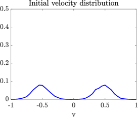
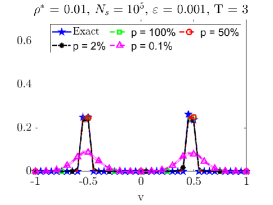
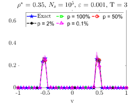
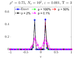
Figure 2: Validation test: comparison between the solution to the kinetic equation in (4.11) computed by means of Asymptotic Nanbu algorithm 4.2 and the exact solution in (4.12). First row, initial solution. Second row, mean (dashed line) and standard deviation (shaded area) of the velocity distribution computed over $S=100$ simulations for different values of $p$. From the left to the right $\rho^{*}=0.01,0.35,0.75$. Markers have been added just to indicate different lines.

In Figure 3 for different values of $\rho^{*}$, the $L_{2}$-norm of the error between the solution to the kinetic equation in (4.11), simulated by means of the Asymptotic Nanbu algorithm 4.2 (one simulation) for different values of $p$, and the exact solution in (4.12). Note that we observe a saturation effect for $\varepsilon\approx 10^{-2}$.

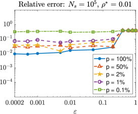
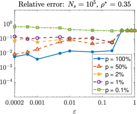
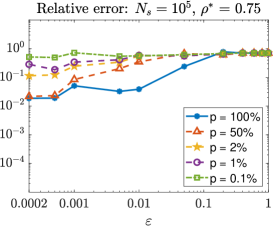
Figure 3: Validation test: $L_{2}$- norm of the error between the solution to the kinetic equation in (4.11) simulated by means of the Asymptotic Nanbu algorithm 4.2 (one simulation) and the exact solution in (4.12). From the left to the right $\rho^{*}=0.01,0.35,1$. Markers represent the error for the different values of $\varepsilon$.

Computational costs.

We now compare the computational costs of the exhaustive search and the $k$–NN search. The computational cost of an exhaustive search is $\mathcal{O}(dN_{s}^{2})$, where $d$ is the space dimension and $N_{s}$ the number of particles. Indeed, first one needs to compute the distances between each point and all the others, with a cost of $\mathcal{O}(dN_{s}^{2})$, and then to sort them, with a cost of $\mathcal{O}(N_{s}^{2}log(N_{s}))$. The cost of a $k$–NN search is logarithmic in time. First one needs to organize agents optimally with a $k$-$d$ tree. The cost of this operation is proportional to $N_{s}log(N_{s})$. Then the idea is to perform a search over the tree to select which are the nearest agents. It can be shown (see [28]) that the $k$–NN search algorithm examines the nodes in optimal order, that is in order of increasing dissimilarities, and that the number of nodes that should be examined is proportional to $((\rho^{*}N_{s})^{1/d}+1)^{d}$. Hence, the total cost to construct a $k$-$d$ tree and to perform the search over it is

$$\mathcal{O}(max(((\rho^{*}N_{s})^{1/d}+1)^{d}log(N_{s}),N_{s}log(N_{s})).$$ (4.13)

In Figure 4 we see the comparison between the computational cost to perform one exhaustive and one $k$–NN search as $N_{s}$ varies for different values of $\rho^{*}$. We set $N_{s}=5\times 10^{3},\ldots,1.5\times 10^{4}$. The $k$–NN computational cost increases as $\rho^{*}$ increases. In Figure 5 we see a comparison between the computational costs of a $k$–NN search as $N_{s}$ varies for different subsamples percentage size $p$. We see that the computational cost decreases proportionally to the subsample size.

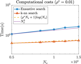
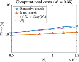
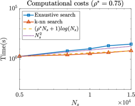
Figure 4: Comparison between the computational costs of the exhaustive search and the $k$–NN search for different values of $N_{s}$. From the left to the right $\rho^{*}=0.01,0.35,0.75$. Markers represent the computational costs relative to the different values of $N_{s}$.

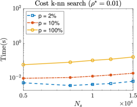
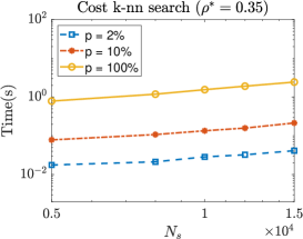
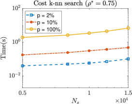
Figure 5: Comparison between the computational costs of the exhaustive search and the $k$–NN search for different values of $N_{s}$ and of the percentage $p$ of the subsample size. From the left to the right $\rho^{*}=0.01,0.35,0.75$. Markers represent the computational costs relative to the different values of $N_{s}$.

5 Numerical experiments

We present different numerical experiments simulating the two and three dimensional dynamics both at the microscopic and mesoscopic levels. The dynamics at microscopic level is discretized by a forward Euler scheme with a time step $\Delta t=0.01$, whereas the evolution of the kinetic dynamics is approximated by the Asymptotic Nanbu algorithm described in 4.2 with $\varepsilon=0.01$. The time evolution of the labels is computed with Algorithm 4.1 at both the microscopic and mesoscopic levels. In the microscopic case we set $N=400$. In the mesoscopic case we choose a sample of $O(N_{s})$ particles, with $N_{s}=5\times 10^{5}$, and a subsample of $O(N_{c})$ particles, with $N_{c}=10^{4}$ that corresponds to a percentage $p=2\%$ of the total mass, for the approximation of the density. We assume the topological target mass to be $\rho^{*}=0.01$. Table 1 reports the parameters of the model that remain unchanged in the various scenarios.

Table 1: Model parameters for the different scenarios.

	$C_{rep}$	$C_{ali}$	$C_{att}$	$C_{v}$	s	$\overline{r}$	$\underline{r}$	$\epsilon$
2D model	100	12	0.7	5	10	200	1	200
3D model	100	12	0.7	5	10	350	20	150

The other parameters will be specified later.

5.1 Numerical test in two spatial dimensions

We consider the swarming dynamics evolving on the spatial space $(x,y)\in\mathbb{R}^{2}$ and velocity space $(v_{x},v_{y})\in\mathbb{R}^{2}$.

5.1.1 Test 2D with no food sources

Suppose the model includes no food sources, i.e. $C_{src}=0$, and no attraction to the centre of mass, i.e. $C_{ctr}=0$. We simulate the dynamics up to time $T=500$, and we report in Figure 6 the initial configuration for both the microscopic and mesoscopic dynamics.

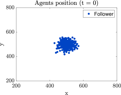
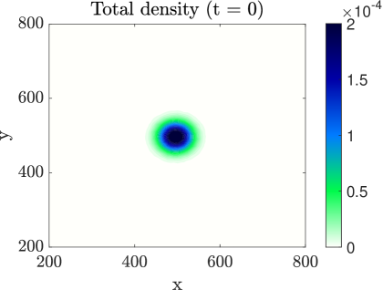
Figure 6: Initial configuration in the spatial 2D case with no food sources.

At time $t=0$, agents are normally distributed with mean $\mu=500$ and variance $\sigma^{2}=25^{2}$ and are in the followers status. Labels change according to the transition rates defined in (3.13) with $q_{FL}=2\times 10^{-4}$ and $q_{LF}=4\times 10^{-3}$.

Microscopic case.

In Figure 7 we report three snapshots of the dynamics at time $t=50$, $t=300$ and $t=500$, for the dynamics without leaders’ emergence (top row) and with leaders’ emergence (bottom row). We observe that, without leaders, agents align and form a compact swarm, whereas with leaders’ emergence we observe the formation of different groups. The splitting is not symmetric since leaders’ emergence occurs randomly and this is reflected in the cluster formation.

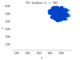
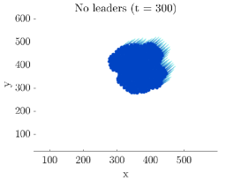
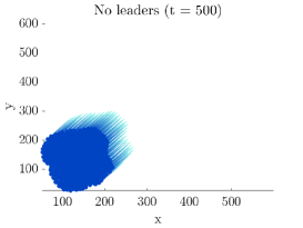
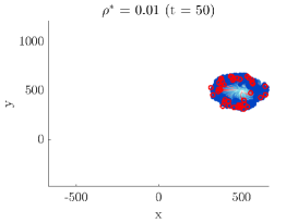
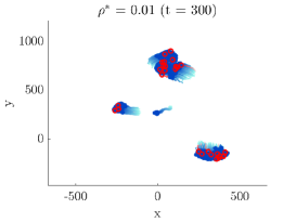
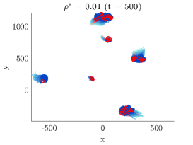
Figure 7: Three snapshots of the 2D dynamics at the microscopic level described in (2.1) with $\lambda$ evolving with rates (3.13) taken at time $t=50$, $t=300$ and $t=500$ and assuming $C_{ctr}=C_{src}=0$. In the first row, the dynamics without leaders. In the second row, the dynamics with leaders assuming $\rho^{*}=0.01$. We represent in blue the agents in the followers status and in red the ones in the leaders status.

Mesoscopic case.

In Figure 8 we report three snapshots of the dynamics at time $t=50$, $t=300$, $t=500$. In the first row, the time evolution of the total density and in red the velocity vector field of the leaders. In the second row, the evolution of the leaders’ density. The behavior is similar to the one of the microscopic case, where we observe the formation of various clusters, and the emergence of leaders uniformly over the swarm density.

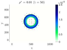
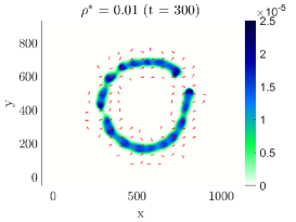
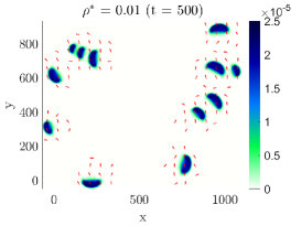
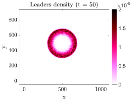
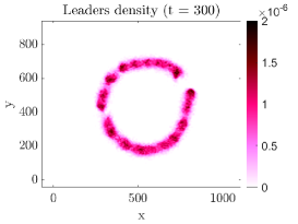
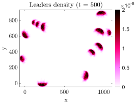
Figure 8: Three snapshots of the 2D dynamics at the mesoscopic level described in (LABEL:eq:boltz_strong) and simulated by means of the Asymptotic Nanbu algorithm 4.2 with $\lambda$ evolving with rates (3.13) as in Algorithm 4.1, taken at time $t=50$, $t=300$ and $t=500$ and assuming $C_{ctr}=C_{src}=0$. In the first row, the dynamics of the total mass and in red the velocity vector field of the leaders. In the second row, the leaders’ dynamics.

In Figure 9 the agents percentages for the dynamics with leaders.

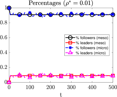
Figure 9: Agents percentages. Markers have been added just to distinguish the different lines.

The videos of the simulations of this subsection are available at [VIDEO].

5.1.2 Test 2D: two food sources

Assume the model includes two food sources located in $x_{1}^{src}=(300,500)$ and $x_{2}^{src}=(1000,500)$. Assume $C_{ctr}=C_{src}=0.75$. Run the dynamics until time $T=200$. In Figure 10 the initial configuration for the microscopic and mesoscopic case. We assume that initially the $87.5\%$ of agents is in the followers status. Among them the $75\%$ is normally distributed with mean $\mu=550$ and variance $\sigma^{2}=10^{2}$ while the $12.5\%$ is normally distributed with mean $\mu=650$ and variance $\sigma^{2}=50^{2}$. The remaining $12.5\%$ is in the leaders status and it is normally distributed with mean $\mu=800$ and variance $\sigma^{2}=10^{2}$. New leaders emerge with higher probability where the followers concentration is higher. Leaders return in the follower status with higher probability if the followers concentration around their position is lower. Hence we consider density dependent transition rates defined in equation (3.16) with $q_{L}=4\times 10^{-3}$ and $q_{F}=3\times 10^{-3}$.

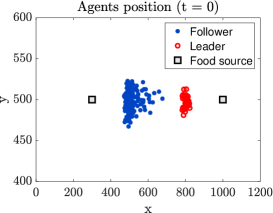
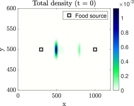
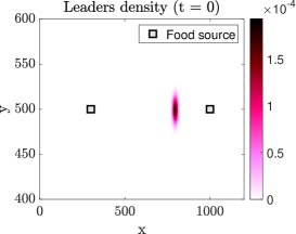
Figure 10: Initial configuration in the 2D case with two food sources.

Microscopic case.

In Figure 11 three snapshots of the dynamics at time $t=50$, $t=100$, $t=200$. Agents that at time $t=0$ were in the leaders status change immediately their labels since no followers are positioned around them. A large group is attracted by one of the two food sources while the remaining part moves subjected just to attraction, repulsion and alignment forces without being attracted by the other food source. Once this smaller group moves far away from the main group, leaders start to be attracted to the centre of mass. In late time, all agents join and move toward one of the two food sources.

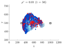
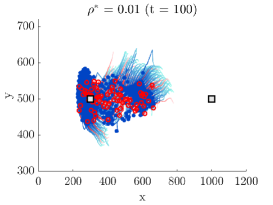
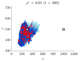
Figure 11: Three snapshots of the 2D dynamics at the microscopic level described in (2.1) with $\lambda$ evolving with rates (3.16) taken at time $t=50$, $t=100$ and $t=200$ and assuming $C_{ctr}=C_{src}=0.75$. We represent in blue the agents in the followers status and in red the ones in the leaders status.

Mesoscopic case.

In Figure 12 three snapshots of the dynamics at time $t=50$, $t=100$, $t=200$. In the first row the time evolution of the total density and in red the velocity vector field of the leaders. In the second row the time evolution of the leaders’ density. The behaviour is similar to the one observed in the microscopic case.

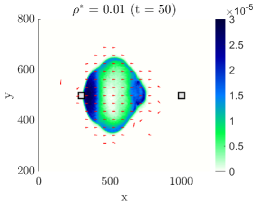
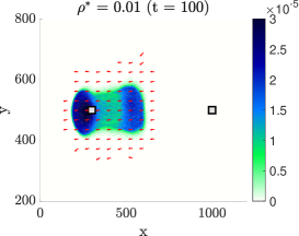
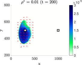
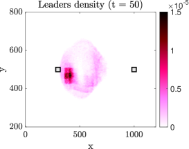
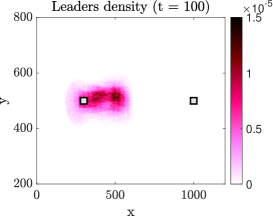
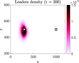
Figure 12: Three snapshots of the 2D dynamics at the mesoscopic level described in (LABEL:eq:boltz_strong) and simulated by means of the Asymptotic Nanbu algorithm 4.2 with $\lambda$ evolving with rates (3.16) as in Algorithm 4.1, taken at time $t=50$, $t=100$ and $t=200$ and assuming $C_{ctr}=C_{src}=0.75$. First row: evolution of the total density and in red the velocity vector field of the leaders’ density. Second row: evolution of the leaders’ density.

In Figure 13 the time evolution of the percentages of leaders and followers for the two dimensional spatial test with two food sources. The agents percentages have been computed both by counting the effective number of followers and leaders per time steps, and as stationary solution to the master equation (3.14). The densities reach the positive equilibrium defined in equation (3.15). Indeed, the transition rates defined in (3.16) can be approximated by constant values. In particular, for any fixed time $t>0$, for any $\lambda\in\{0,1\}$ and for any $x\in\mathbb{R}^{d}$ we have

$$\pi_{L\to F}(x,\lambda;f,t)=\bar{\alpha}(t),\qquad\pi_{F\to L}(x,\lambda;f,t)=\bar{\beta}(t)$$ (5.1)

where

$$\bar{\alpha}(t)=\mathbb{E}_{x}\left(\pi_{L\to F}(\cdot)\right),\qquad\bar{\beta}(t)=\mathbb{E}_{x}\left(\pi_{F\to L}(\cdot)\right),$$ (5.2)

with $\mathbb{E}_{x}(\cdot)$ denoting the mean value with respect to $x$.
Similar results can be obtained for the 2D model without food sources since the transition rates are constants values, by definition.

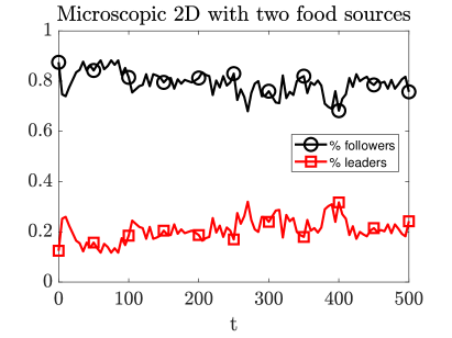
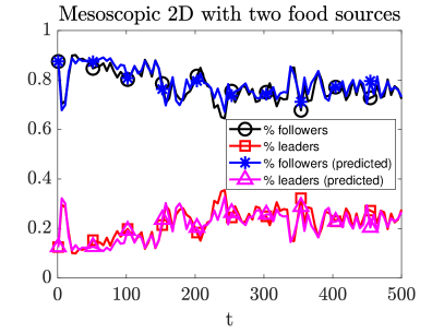
Figure 13: Agents percentages: microscopic (on the left) and mesoscopic (on the right) two dimensional model with two food sources. In black and in red the agents percentages computed by counting the effective number of followers and leaders per time steps. In blue and in magenta the stationary solution to the master equation (3.14).

The videos of the simulations of this subsection are available at [VIDEO].

5.1.3 Test 2D: one food source

Assume the model includes one food source located in $x_{1}^{src}=(300,500)$. Run the simulation until time $T=120$. Suppose labels change aiming at organizing agents toward a common target, that in this case is supposed to be the food source $x_{1}^{src}$. In particular, assume $\lambda$ varies with rates (3.18) with $\bar{\alpha}=0.7$ and $\underline{\alpha}=0.3$. In Figure 14 the initial configuration for both the microscopic and mesoscopic case.

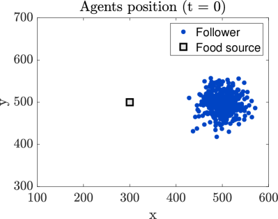
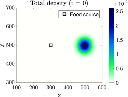
Figure 14: Initial configuration in the 2D case with one food source.

Microscopic case.

In Figure 15 three snapshots of the dynamics at time $t=5$, $t=20$ and $t=50$ with leaders and with $\mathcal{G}[f](\cdot)$ chosen as in (3.20). Followers are driven by leaders and reach the target position.

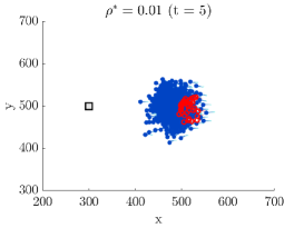
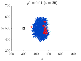
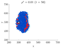
Figure 15: Three snapshots of the 2D dynamics at the microscopic level described in (2.1) with $\lambda$ evolving with rates (3.18) taken at time $t=5$, $t=20$ and $t=50$ and assuming $C_{ctr}=C_{src}=0$. We represent in blue the agents in the followers status and in red the ones in the leaders status.

Mesoscopic case.

In Figure 16 three snapshots of the dynamics at time $t=5$, $t=20$, $t=50$ with transition rates depending on the orientation according to (3.18). In the first row, the evolution of the whole mass, and in red the velocity vector field of the leaders. In the second row, the evolution of the leaders mass.

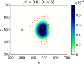
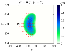
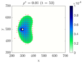
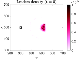
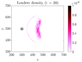
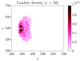
Figure 16: Three snapshots of the 2D dynamics at the mesoscopic level described in (LABEL:eq:boltz_strong) and simulated by means of the Asymptotic Nanbu algorithm 4.2 with $\lambda$ evolving with rates (3.18) as in Algorithm 4.1, taken at time $t=5$, $t=20$ and $t=50$ and assuming $C_{ctr}=C_{src}=0$. First row: evolution of the total density and in red the velocity vector field of the leaders. Second row: evolution of the leaders density.

In Figure 17 we report in the first row the angle velocity distribution at time $t=100$, $t=120$, $t=180$ and in the second row the correspondent velocity vector field, outlining the milling behaviour around the target positions $\overline{x}=x_{1}^{src}$.

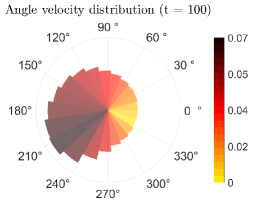
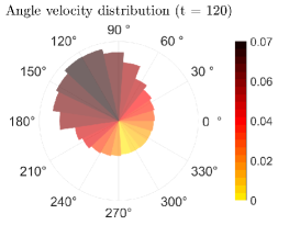
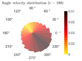
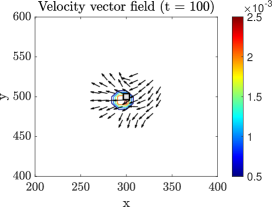
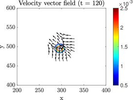
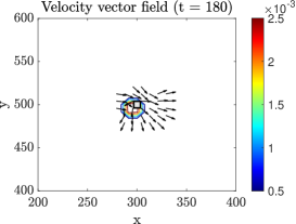
Figure 17: Angle velocity distribution (first row) and velocity vector field (second row) at time $t=100$, $t=120$, $t=180$ obtained by simulating the dynamics in (LABEL:eq:boltz_strong) by means of the algorithm 4.2 with $\lambda$ evolving with rates (3.18) as in algorithm 4.1.

The videos of the simulations of this subsection are available at [VIDEO].

5.2 Numerical test in 3D with two food sources

We consider the three dimensional model in space and velocity, simulating the swarming dynamics up time $T=200$. Initially agents are normally distributed with mean $\mu=500$ and variance $\sigma^{2}=25^{2}$ in both spatial and velocity dimension, and are all in the followers status. We report in Figure 18 the initial configuration for both the microscopic and mesoscopic case. For the mesoscopic case, we also depict on the $(x,y)$ plane the projection of the spatial density.

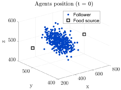
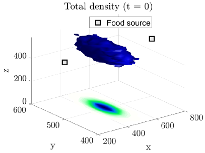
Figure 18: Initial configuration in the 3D case with food sources.

Assume the two food sources to be located in $x_{1}^{src}=(200,500,500)$ and $x_{2}^{src}=(800,500,500)$. Suppose that leaders emerge with density-dependent transition rates as defined in (3.16) and where we assume the constants to be $q_{L}=4\times 10^{-3}$ and $q_{F}=3\times 10^{-3}$.

Microscopic case.

In Figure 19 three snapshots of the dynamics at time $t=50$, $t=100$, $t=200$. First row: $C_{centre}=0$, $C_{food}=0.75$. Agents split in two groups moving toward the two food sources. Second row: $C_{ctr}=4$, $C_{src}=0.75$. At final time agents move toward one of the two food sources.

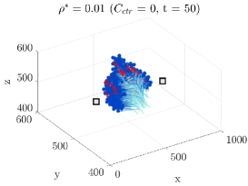
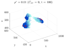
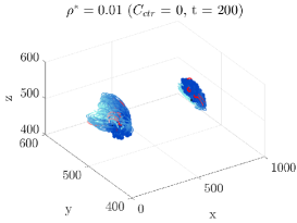
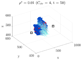
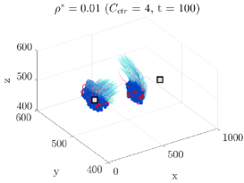
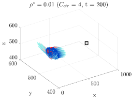
Figure 19: Three snapshots of the 3D dynamics at the microscopic level described in (2.1) with $\lambda$ evolving with rates (3.16) taken at time $t=50$, $t=100$ and $t=200$. First row, $C_{ctr}=0$, $C_{src}=0.75$. Second row, $C_{ctr}=4$, $C_{src}=0.75$. We represent in blue the agents in the followers status and in red the ones in the leaders status.

Mesoscopic case.

In Figure 20 we report three snapshots of the dynamics at time $t=50$, $t=100$, $t=200$ and in red the velocity vector field. We add also the density distribution of the whole flock projected over the plane $(x,y)$ and in red the leaders velocity vector field. First row: $C_{crt}=0$, $C_{src}=0.75$. Second row: $C_{ctr}=4$, $C_{src}=0.75$. The behaviour is similar to the one in the microscopic case.

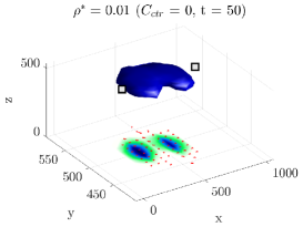
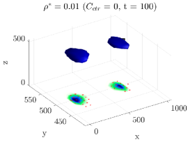
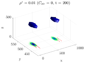
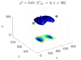
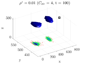
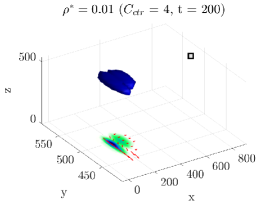
Figure 20: Three snapshots of the 3D dynamics at the mesoscopic level described in (LABEL:eq:boltz_strong) and simulated by means of the Asymptotic Nanbu algorithm 4.2 with $\lambda$ evolving with rates (3.16) as in Algorithm 4.1, taken at time $t=50$, $t=100$ and $t=200$. First row, $C_{ctr}=0$, $C_{src}=0.75$. Second row, $C_{ctr}=4$, $C_{src}=0.75$. In red the velocity vector field.

The videos of the simulations of this subsection are available at [VIDEO].

6 Conclusions

In this paper, we have studied collective behaviour of birds under a follower-leaders dynamics, starting from a simplified version of the model presented in [20].Through the emergence of leaders, we recover the ability to split the initial configuration and initiate directional changes without the need of external influences. We derived a kinetic model to effectively depict the motion of a large swarm with transient leadership and topological interactions, and subsequently we simulated the dynamics introducing a novel stochastic particle method. A significant emphasis was placed on studying topological interactions. We tackled the issue of the numerical evaluation of nearest Neighbors reducing the computational costs of the search from quadratic to logarithmic by optimally organizing agents in a binary tree and performing a $k$-NN search. Moreover, we directed our attention to transient leadership, showcasing how labels can change over time, particularly for driving agents towards a common target. Various strategies for leaders’ emergence were explored, including continuous leadership levels, as introduced in Remark 1. Additionally, it would be intriguing to describe the original model from a kinetic viewpoint, reintroducing delay, which, as demonstrated in [20], appears to play a crucial role in achieving desired configurations. Finally, several questions arise concerning the study of non-local terms in high dimensions. For instance, it could be beneficial to further enhance the numerical scheme implemented, focusing on other useful strategies for approximating topological interactions.

References

- [1] G. Albi, S. Almi, M. Morandotti, and F. Solombrino. Mean-field selective optimal control via transient leadership. Applied Mathematics & Optimization, 85(2):22, 2022.
- [2] G. Albi, N. Bellomo, L. Fermo, S.-Y. Ha, J. Kim, L. Pareschi, D. Poyato, and J. Soler. Vehicular traffic, crowds, and swarms: From kinetic theory and multiscale methods to applications and research perspectives. Mathematical Models and Methods in Applied Sciences, 29(10):1901–2005, 2019.
- [3] G. Albi, M. Bongini, E. Cristiani, and D. Kalise. Invisible control of self-organizing agents leaving unknown environments. SIAM Journal on Applied Mathematics, 76(4):1683–1710, 2016.
- [4] G. Albi, M. Bongini, F. Rossi, and F. Solombrino. Leader formation with mean-field birth and death models. Mathematical Models and Methods in Applied Sciences, 29(04):633–679, 2019.
- [5] G. Albi and L. Pareschi. Binary interaction algorithms for the simulation of flocking and swarming dynamics. Multiscale Modeling & Simulation, 11(1):1–29, 2013.
- [6] G. Albi, L. Pareschi, and M. Zanella. Opinion dynamics over complex networks: Kinetic modelling and numerical methods. Kinetic & Related Models, 10(1):1, 2017.
- [7] M. Ballerini, N. Cabibbo, R. Candelier, A. Cavagna, E. Cisbani, I. Giardina, A. Orlandi, G. Parisi, A. Procaccini, M. Viale, et al. Empirical investigation of starling flocks: a benchmark study in collective animal behaviour. Animal behaviour, 76(1):201–215, 2008.
- [8] D. Benedetto, E. Caglioti, and S. Rossi. Mean-field limit for particle systems with topological interactions. Mathematics and Mechanics of Complex Systems, 9(4):423–440, 2022.
- [9] S. Bernardi, A. Colombi, and M. Scianna. A particle model analysing the behavioural rules underlying the collective flight of a bee swarm towards the new nest. Journal of biological dynamics, 12(1):632–662, 2018.
- [10] S. Bernardi, R. Eftimie, and K. J. Painter. Leadership through influence: what mechanisms allow leaders to steer a swarm? Bulletin of Mathematical Biology, 83(6):69, 2021.
- [11] S. Bidari, O. Peleg, and Z. P. Kilpatrick. Social inhibition maintains adaptivity and consensus of honeybees foraging in dynamic environments. Royal Society open science, 6(12):191681, 2019.
- [12] A. Blanchet and P. Degond. Topological interactions in a Boltzmann-type framework. Journal of Statistical Physics, 163:41–60, 2016.
- [13] A. Blanchet and P. Degond. Kinetic models for topological nearest-neighbor interactions. Journal of Statistical Physics, 169(5):929–950, 2017.
- [14] E. Bonabeau, G. Theraulaz, J.-L. Deneubourg, S. Aron, and S. Camazine. Self-organization in social insects. Trends in ecology & evolution, 12(5):188–193, 1997.
- [15] A. Bressan, S. Čanić, M. Garavello, M. Herty, and B. Piccoli. Flows on networks: recent results and perspectives. EMS Surveys in Mathematical Sciences, 1(1):47–111, 2014.
- [16] J. Carrillo, L. Pareschi, and M. Zanella. Particle based gPC methods for mean-field models of swarming with uncertainty. Communications in Computational Physics, 25(2):508–531, 2019.
- [17] J. A. Carrillo, M. Fornasier, G. Toscani, and F. Vecil. Particle, kinetic, and hydrodynamic models of swarming. Mathematical modeling of collective behavior in socio-economic and life sciences, pages 297–336, 2010.
- [18] Y.-P. Choi, D. Kalise, J. Peszek, and A. A. Peters. A collisionless singular Cucker–Smale model with decentralized formation control. SIAM Journal on Applied Dynamical Systems, 18(4):1954–1981, 2019.
- [19] E. Cristiani, N. Loy, M. Menci, and A. Tosin. Kinetic and macroscopic description of flocking dynamics with continuous leader-follower transition. preprint, 2023.
- [20] E. Cristiani, M. Menci, M. Papi, and L. Brafman. An all-leader agent-based model for turning and flocking birds. Journal of Mathematical Biology, 83(4):1–22, 2021.
- [21] E. Cristiani, B. Piccoli, and A. Tosin. Multiscale modeling of pedestrian dynamics, volume 12. Springer, 2014.
- [22] F. Cucker and S. Smale. Emergent behavior in flocks. IEEE Transactions on automatic control, 52(5):852–862, 2007.
- [23] P. Degond and M. Pulvirenti. Propagation of chaos for topological interactions. The Annals of Applied Probability, 29(4):2594–2612, 2019.
- [24] G. Dimarco, L. Pareschi, G. Toscani, and M. Zanella. Wealth distribution under the spread of infectious diseases. Physical Review E, 102(2):022303, 2020.
- [25] A. Dussutour, S. C. Nicolis, J.-L. Deneubourg, and V. Fourcassié. Collective decisions in ants when foraging under crowded conditions. Behavioral Ecology and Sociobiology, 61:17–30, 2006.
- [26] M. R. D’ÄôOrsogna, Y.-L. Chuang, A. L. Bertozzi, and L. S. Chayes. Self-propelled particles with soft-core interactions: patterns, stability, and collapse. Physical review letters, 96(10):104302, 2006.
- [27] M. Fornasier, J. Haskovec, and G. Toscani. Fluid dynamic description of flocking via the Povzner–Boltzmann equation. Physica D: Nonlinear Phenomena, 240(1):21–31, 2011.
- [28] J. H. Friedman, J. L. Bentley, and R. A. Finkel. An algorithm for finding best matches in logarithmic expected time. ACM Transactions on Mathematical Software (TOMS), 3(3):209–226, 1977.
- [29] J. Haskovec. Flocking dynamics and mean-field limit in the Cucker–Smale-type model with topological interactions. Physica D: Nonlinear Phenomena, 261:42–51, 2013.
- [30] C. K. Hemelrijk and H. Hildenbrandt. Self-organized shape and frontal density of fish schools. Ethology, 114(3):245–254, 2008.
- [31] A. Jadbabaie, J. Lin, and A. S. Morse. Coordination of groups of mobile autonomous agents using nearest neighbor rules. IEEE Transactions on automatic control, 48(6):988–1001, 2003.
- [32] S. Jin, L. Li, and J.-G. Liu. Random batch methods (RBM) for interacting particle systems. Journal of Computational Physics, 400:108877, 2020.
- [33] A. J. King, S. J. Portugal, D. Strömbom, R. P. Mann, J. A. Carrillo, D. Kalise, G. de Croon, H. Barnett, P. Scerri, R. Groß, et al. Biologically inspired herding of animal groups by robots. Methods in Ecology and Evolution, 14(2):478–486, 2023.
- [34] A. L. Koch and D. White. The social lifestyle of myxobacteria. Bioessays, 20(12):1030–1038, 1998.
- [35] Z. Li and S.-Y. Ha. On the Cucker-Smale flocking with alternating leaders. Quarterly of Applied Mathematics, 73(4):693–709, 2015.
- [36] N. Loy and A. Tosin. Boltzmann-type equations for multi-agent systems with label switching. Kinetic & Related Models, 14, 2021.
- [37] R. Lukeman, Y.-X. Li, and L. Edelstein-Keshet. Inferring individual rules from collective behavior. Proceedings of the National Academy of Sciences, 107(28):12576–12580, 2010.
- [38] M. Morandotti and F. Solombrino. Mean-field analysis of multipopulation dynamics with label switching. SIAM Journal on Mathematical Analysis, 52(2):1427–1462, 2020.
- [39] K. Nanbu. Theoretical basis of the direct simulation Monte Carlo method. In 15th International Symposium on Rarefied Gas Dynamics, volume 1, pages 369–383, 1986.
- [40] L. Pareschi and G. Russo. Time relaxed Monte Carlo methods for the boltzmann equation. SIAM Journal on Scientific Computing, 23(4):1253–1273, 2001.
- [41] L. Pareschi and G. Toscani. Interacting multiagent systems: kinetic equations and Monte Carlo methods. OUP Oxford, 2013.
- [42] J. K. Parrish and L. Edelstein-Keshet. Complexity, pattern, and evolutionary trade-offs in animal aggregation. Science, 284(5411):99–101, 1999.
- [43] A. Y. Povzner. On the Boltzmann equation in the kinetic theory of gases. Matematicheskii Sbornik, 100(1):65–86, 1962.
- [44] H. Rainer and U. Krause. Opinion dynamics and bounded confidence: models, analysis and simulation. 2002.
- [45] G. Toscani. Kinetic models of opinion formation. Communications in mathematical sciences, 4(3):481–496, 2006.