Data-Induced Interactions of Sparse Sensors

Abstract

Large-dimensional empirical data in science and engineering frequently has low-rank structure and can be represented as a combination of just a few eigenmodes. Because of this structure, we can use just a few spatially localized sensor measurements to reconstruct the full state of a complex system. The quality of this reconstruction, especially in the presence of sensor noise, depends significantly on the spatial configuration of the sensors. Multiple algorithms based on gappy interpolation and QR factorization have been proposed to optimize sensor placement. Here, instead of an algorithm that outputs a singular “optimal” sensor configuration, we take a thermodynamic view to compute the full landscape of sensor interactions induced by the training data. The landscape takes the form of the Ising model in statistical physics, and accounts for both the data variance captured at each sensor location and the crosstalk between sensors. Mapping out these data-induced sensor interactions allows combining them with external selection criteria and anticipating sensor replacement impacts.

Many natural and engineered systems can take a variety of high-dimensional states, with the amount of data growing rapidly with the number of observed snapshots and increasing snapshot resolution. At the same time, the amount of information in this data usually grows much slower, often logarithmically [1, 2, 3]. In this situation, any system state can be closely approximated by a combination of just a few basis vectors, enabling algorithms from lossy image compression to Dynamic Mode Decomposition [4, 5]. While the optimal basis can be learned from historical data or high-fidelity simulations, states cannot be measured in that basis directly and often can only be accessed by spatially-localized sensors.

Reconstruction of full states from localized sensor measurements has a long history under the umbrella term of compressed sensing, where the sampling points (sensor locations) are chosen randomly and the state is reconstructed as a sparse combination of universal basis vectors [6, 7, 8]. More recently, driven by advances in gappy and reduced-order PDE methods [9, 10, 11], sparse sensing algorithms have been developed to take advantage of the available training data to reduce the number of sensors required for given reconstruction quality [12]. The general sparse sensing problem is usually set up as follows: given the training data matrix $X$ consisting of $N$ snapshots of an $n$-dimensional state, one needs to reconstruct an unknown state $\vec{x}\in\mathbb{R}^{n}$ sampled from the same distribution as the data by using only the noisy measurements of a few components of the state $\vec{y}\in\mathbb{R}^{p},p\ll n$.

While any combination of sensors of appropriate rank can be used to compute the maximal likelihood state reconstruction, the reconstruction robustness to sensor noise may vary by orders of magnitude, leading to the problem of sensor placement. Each sensor configuration can be assigned a cost function value that can be approximately maximized with efficient greedy heuristics based on optimal experiment design, information theory metrics, Gibbs sampling, or matrix QR pivoting [13, 14, 15, 16, 12]. While these methods return a sensor configuration provably close to the true optimum due to the submodularity property [17, 18, 19], they do not inform why a particular configuration should be chosen, how to best modify it if sensor budget changes, and what would be the impact of a sensor malfunction on the reconstruction quality.

In this paper, instead of searching for a singular “optimal” configuration of sensors, we take a thermodynamic perspective to study the entire landscape of sensor interactions, akin to saliency maps in machine vision [20]. We show that the sensor interactions can be interpreted in terms of 1-body, 2-body, and higher order Hamiltonian terms computed directly from the training data. Understanding the part of the landscape induced by data directly inspires a greedy sensor placement algorithm, allows incorporating landscapes driven by external cost factors, and anticipates the impacts of sensor replacement needs. The energy landscape analysis can be combined with other recent advances in sensor placement studies.

State reconstruction algorithm.

The training library can be represented via Proper Orthogonal Decomposition (POD) and closely approximated via POD truncation:

$$X=\Psi\Sigma V^{T}\approx\Psi_{r}\Sigma_{r}V_{r}^{T},$$ (1)

where we dropped all singular values beyond the first $r$ per the optimal truncation prescription [3]. In the reduced basis any state can be approximated as a linear combination of data-driven basis vectors $\vec{x}\approx\Psi_{r}\vec{a}$.

Our goal is to estimate the coefficients $\hat{\vec{a}}$ from the spatially-localized measurements $\vec{y}=C\vec{x}+\xi$, where $C$ is a $p\times n$ selection matrix consisting of $p$ rows of the identity matrix and $\xi$ is Gaussian uncorrelated sensor measurement noise with magnitude $\eta$. Given this measurement model and a Gaussian prior distribution of the coefficients $\vec{a}$ parameterized by the variances $S$, we derive the following maximal likelihood reconstruction:

$$\hat{\vec{a}}=\left(S^{-2}+\frac{\Theta^{T}\Theta}{\eta^{2}}\right)^{-1}\frac{\Theta^{T}\vec{y}}{\eta^{2}}=A^{-1}\frac{\Theta^{T}\vec{y}}{\eta^{2}};\;\hat{\vec{x}}=\Psi_{r}\hat{\vec{a}}$$ (2)

valid for any choice of sensors $C$ and sensor readings $\vec{y}$, with $\Theta=C\Psi_{r}$. However, the accuracy and noise sensitivity of this reconstruction depend dramatically on the properties of the sensor-dependent matrix $A$, and thus requires a strategy to place sensors systematically.

Sensor placement landscapes.

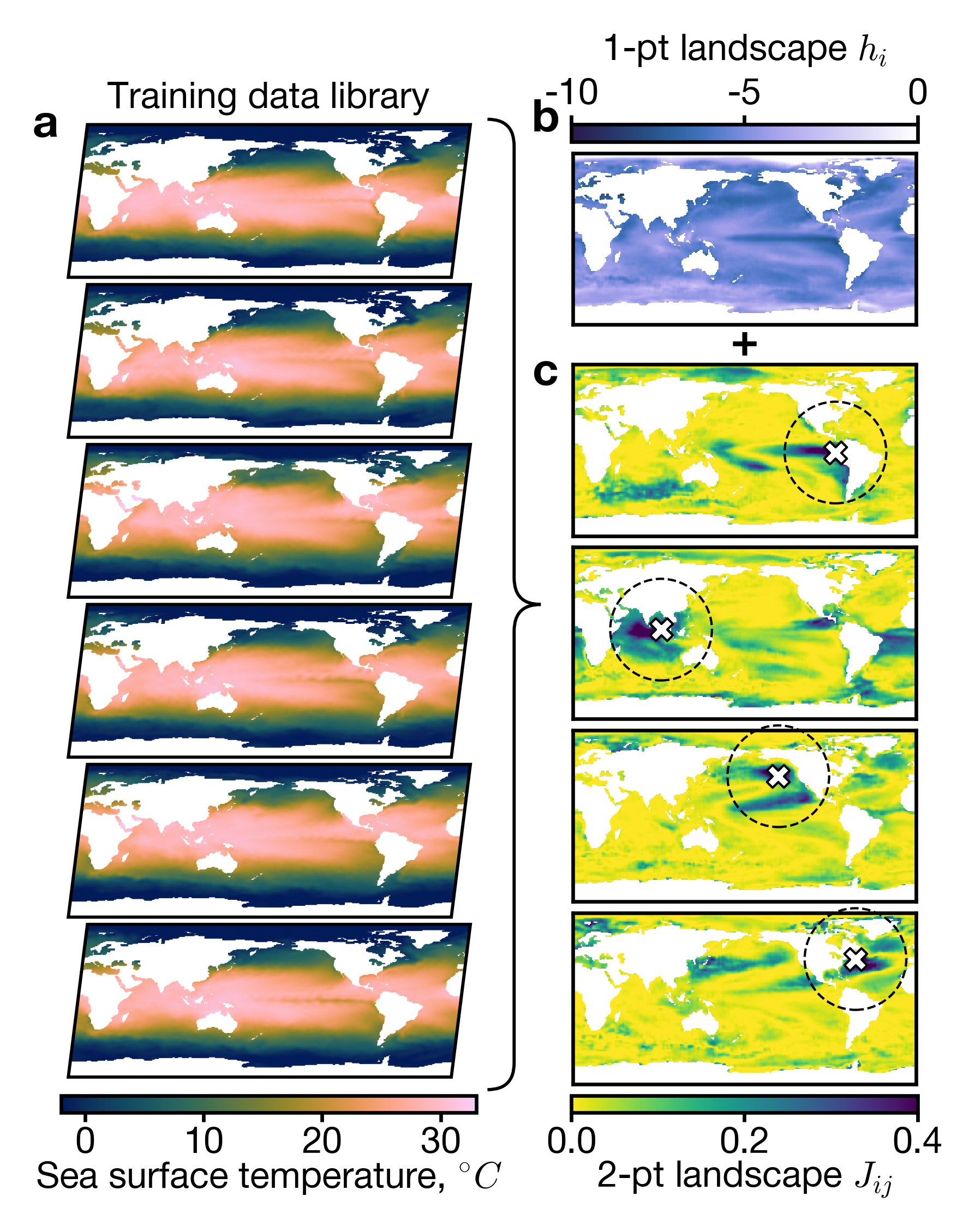
Figure 1: Computation of the sensor placement landscape from the training data library. (a) A collection of data snapshots of identical dimensions, here the Sea Surface Temperature data set. (b) The library is used to compute the sensor placement landscape to multiple orders, here showing the 1-point landscape at each location $h_{i}$ and the 2-point landscape $J_{ij}$ conditioned on the sensor locations marked with white crosses and highlighted with dashed circles.

The reconstruction error of Eqn. 2 can be measured by various scalar functions of the matrix $A$, most commonly its determinant, in an approach known as D-optimal design [13]. The determinant is an attractive optimization target because it characterizes the uncertainty hypervolume of the reconstruction, its maximum can be approximated with the QR decomposition [12], and the submodularity property guarantees the near-optimality of greedy optimization [17, 18, 19].

In this paper we identify the (negative) determinant of the inversion matrix with the energy or Hamiltonian of a particular set of sensors $\gamma$. The resulting Hamiltonian is remarkably similar to the Ising model found across statistical physics:

$$\mathcal{H}(\gamma)\equiv -\ln(\det A)\approx E_{b}+\sum\limits_{i\in\gamma}h_{i}+\sum\limits_{i\neq j\in\gamma}J_{ij}$$ (3)

$$h_{i}\equiv -\ln(1+\vec{g}_{i}\cdot\vec{g}_{i}/\eta^{2})\leq 0$$ (4)

$$J_{ij}\equiv \frac{1}{2}\frac{(\vec{g}_{i}\cdot\vec{g}_{j}/\eta^{2})^{2}}{(1+\vec{g}_{i}\cdot\vec{g}_{i}/\eta^{2})(1+\vec{g}_{j}\cdot\vec{g}_{j}/\eta^{2})}\geq 0,,$$ (5)

where $\vec{g}_{i}$ are the sensing vectors describing the sensitivity of each possible sensor location to each of the POD modes, computed as rows of the data-driven matrix $G=\Psi_{r}S$. The functional form of $h_{i}$ and $J_{ij}$ is computed via series expansion of the matrix $A$ in powers of $\eta$ (Eqn. 2) and resummation, similar to enumeration arguments in self-assembly studies [21, 22] (see Supplementary Materials for derivation).

In the Hamiltonian formulation of sensor placement 3, the objective depends on the locations of individual sensors and sensor pairs from the chosen set $\gamma$ (Fig. 1). Qualitatively, minimizing the Hamiltonian requires picking sensors $i\in\gamma$ that capture a lot of signal variance (large $\vec{g}_{i}\cdot\vec{g}_{i}$), but are not very correlated with each other (small $\vec{g}_{i}\cdot\vec{g}_{j}$). While a combinatorial search for the lowest energy configuration would require evaluating the $\order{n^{2}}$ elements of the full crosstalk $\mathbf{J}$ matrix, we propose a simple greedy “2-point” algorithm that minimizes the marginal energy of each next placed sensor:

$$q=\arg\min\limits_{q}\left(h_{q}+2\sum\limits_{i\in\gamma}J_{iq}\right);\;\gamma\leftarrow q,$$ (6)

requiring just $\order{p\cdot n}$ evaluations to place $p\ll n$ sensors.

Reconstruction progress.

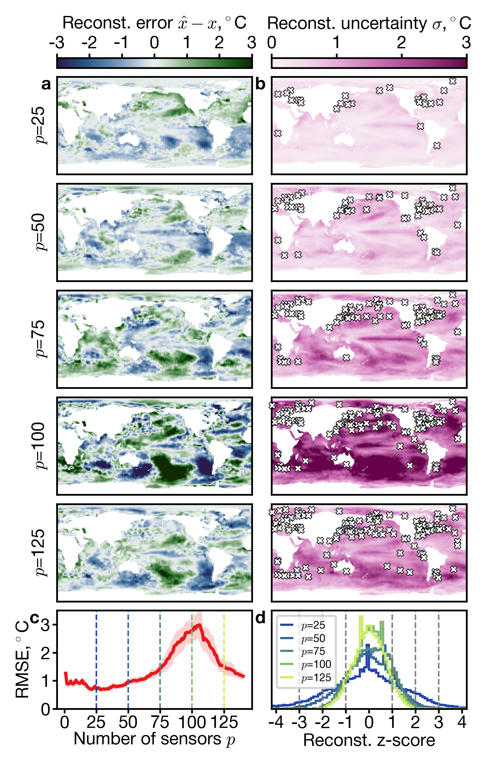
Figure 2: State reconstruction with progressively more sensors $p$ at noise level $\eta=1.0^{\circ}C$. (a) Reconstruction error between the maximal likelihood reconstructed state and the true state. (b) Uncertainty heatmaps of the reconstruction and the sensor locations chosen by the 2-point algorithm (white crosses). (c) RMSE of the reconstruction with the solid curve and the shaded region showing mean $\pm$ one standard deviation across 20 realizations of sensor noise. The RMSE peak corresponds to the model dimension, here $r=100$. (d) Distribution of reconstruction z-scores at every pixel $z_{i}=(\hat{x}_{i}-x_{i})/\sigma_{i}$

We demonstrate the sensor placement algorithm on an example dataset of weekly average sea surface temperature (SST) between 1990 and 2023 [23], truncated to POD rank $r=100$. Each frame covers the entirety of Earth surface in equirectangular projection at $1^{\circ}$ resolution, resulting in $360\times 180$ pixel images with $n=44219$ pixels corresponding to sea surface. We show that by employing as few as 25 sensors selected by the 2-point algorithm with noise level of $\eta=1^{\circ}C$, the entire temperature field can be reconstructed to within $1^{\circ}C$ (Fig. 2a). The reconstruction method also provides an Uncertainty Quantification (UQ) method in form of the uncertainty heat map at every pixel (Fig. 2b). Uncertainty is lowest close to the selected sensors, primarily around continents and within inland bodies of water, and highest in southern parts of the Indian, Pacific, and Atlantic Oceans. We emphasize that the sensor placement algorithm was trained exclusively on the snapshot library, with no additional information about the structure of Earth’s oceans or their physical processes.

The reconstruction Root Mean Square Error (RMSE) shows non-monotonic dependence on the number of sensors (Fig. 2c). While adding more sensors contributes more information to the reconstruction algorithm, it also trades off with the number of independent sources of noise, resulting in best performance at $p\sim 25$ for sensor noise of $\eta=1.0^{\circ}C$. Importantly, the RMSE peaks at $p\sim r=100$ since the model cannot reconstruct the features in the truncated POD modes. Since both the reconstruction error and reconstruction uncertainty increase with sensor number, we assess the model confidence by computing the z-score of each individual pixel $z_{i}=(\hat{x}_{i}-x_{i})/\sigma_{i}$ and plotting its distribution (Fig. 2d). Across all sensor numbers, the z-score distribution is symmetric and concentrated within $z\in[-3,3]$, indicating that the reconstruction does not systematically over- or under-estimate the temperature, and provides an accurate estimation of the uncertainty.

Reconstruction diagnostics

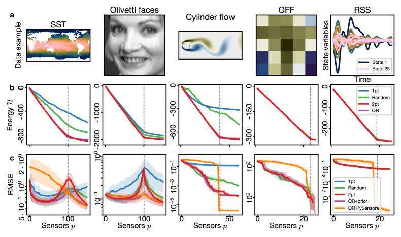
Figure 3: Comparison of reconstruction metrics for different datasets, with 4:1 train/test split. (a) Examples of dataset snapshots for different systems. The RSS dataset is non-spatial, so temporal trajectories are shown instead. (b) Exact energies of sensor configurations selected with different methods: random placement, 1-point algorithms, 2-point algorithm, and QR pivoting. (c) Root mean square error (RMSE) of state reconstruction, with solid line and shaded region indicating average $\pm$ 1 standard deviation across the test set. The vertical dashed line indicates the number of modes $r$ used in the reconstruction.

We compute sensor placement and reconstruction error across five datasets and four sensor placement methods. Apart from the SST dataset, we use the Olivetti faces dataset [24], snapshots of a numerical simulation of flow past a cylinder [25, 26], as well as synthetic Gaussian Free Field [27] and Random State System [28] datasets (Fig. 3a, see SM for dataset details). The four sensor placement algorithms are: random, 1-point (minimizing $h_{q}$ only), 2-point (Eqn. 6), and QR-based [29]. For the QR sensors, we compute reconstruction with and without the prior regularization. For each dataset, the sensor placement landscape is derived from the training set with 80% of the data, and the reconstruction error is computed across the test set with the remaining 20% of the data.

For the three empirical datasets (SST, Olivetti, and cylinder) the random and 1-point algorithms have higher energies than the other two (Fig. 3b). The 1-point algorithm has higher RMSE than other reconstructions with prior, highlighting the importance of crosstalk for sensor placement (Fig. 3c). The QR sensors without prior regularization also show consistently higher RMSE, justifying the need for a prior. The regularized random, 2-point, and QR algorithms show nearly equivalent RMSE error curves, all showing the peak at $p\sim r$ due to the POD mode truncation. For the two synthetic datasets all sensor placement methods have nearly equivalent performance, but can also be compared to brute force search (see SM). We conclude that while the 2-point and the QR algorithms are based on the same underlying POD modes and have nearly equivalent numerical performance, the 2-point algorithm provides much richer interpretation in terms of sensor landscapes and interactions.

Conclusions and outlook.

The key advance of this paper is casting the sensor selection problem in thermodynamic terms of interaction energies of progressively larger numbers of sensors. While we focus the discussion on the 1-body and 2-body interactions, the mathematical formalism extends to any higher number (see SM). The shape of the 2-body interactions can be further connected to the properties of the physical, mathematical, or even artistic processes that generate data [30, 31, 32]. We used a greedy 2-point method of sensor placement in order to limit the required memory and computing time, but if the whole landscape could fit in memory, better energy minima can be obtained through methods such as gradient descent or simulated annealing [33]. Due to the usage of a regularizing prior, state reconstruction can be consistently performed for any number of sensors without the requirement that $p\geq r$ [12].

While the sensor landscape approach provides interpretability and in some regimes selects better sensor sets than state-of-the-art approaches, it is ultimately followed by a linear algorithm for reconstructing the state from sensor readings, limiting the reconstruction accuracy. Recent work has shown that a linear algorithm of sensor selection based on QR factorization can be combined with a nonlinear shallow decoder network state estimation, which nevertheless requires neural network retraining for any new sensor set [34]. An alternative approach instead focuses on learning the data manifold geometry and identifying nonlinear coordinates [19], which would be equivalent to replacing the Gaussian prior in our approach with a more complex one. Other sensor placement extensions can involve estimation of time-dependent dynamics through Kalman filtering [35], or sensors advected by the flows they are trying to measure [36]. Finally, the approach here identifies only the part of sensor placement landscape induced by the training data, which can be combined with other design objectives such as placement cost or restrictions [37, 38, 39, 40].

The authors would like to thank S.E. Otto and J. Williams for helpful discussions and L.D. Lederer for administrative support. This work uses Scientific Color Maps for visualization [41]. The authors acknowledge support from the National Science Foundation AI Institute in Dynamic Systems (grant number 2112085).

References

- Quinn et al. [2022] K. N. Quinn, M. C. Abbott, M. K. Transtrum, B. B. Machta, and J. P. Sethna, Information geometry for multiparameter models: New perspectives on the origin of simplicity, Reports on Progress in Physics (2022).
- Udell and Townsend [2019] M. Udell and A. Townsend, Why are big data matrices approximately low rank?, SIAM Journal on Mathematics of Data Science 1, 144 (2019).
- Gavish and Donoho [2014] M. Gavish and D. L. Donoho, The optimal hard threshold for singular values is , IEEE Transactions on Information Theory 60, 5040 (2014).
- Kutz et al. [2016] J. N. Kutz, S. L. Brunton, B. W. Brunton, and J. L. Proctor, Dynamic mode decomposition: data-driven modeling of complex systems (SIAM, 2016).
- Lewis and Knowles [1992] A. S. Lewis and G. Knowles, Image compression using the 2-d wavelet transform, IEEE Transactions on image Processing 1, 244 (1992).
- Donoho [2006] D. L. Donoho, Compressed sensing, IEEE Transactions on information theory 52, 1289 (2006).
- Ganguli and Sompolinsky [2010] S. Ganguli and H. Sompolinsky, Statistical mechanics of compressed sensing, Physical review letters 104, 188701 (2010).
- Krzakala et al. [2012] F. Krzakala, M. Mézard, F. Sausset, Y. Sun, and L. Zdeborová, Statistical-physics-based reconstruction in compressed sensing, Physical Review X 2, 021005 (2012).
- Everson and Sirovich [1995] R. Everson and L. Sirovich, Karhunen–loeve procedure for gappy data, JOSA A 12, 1657 (1995).
- Barrault et al. [2004] M. Barrault, Y. Maday, N. C. Nguyen, and A. T. Patera, An ‘empirical interpolation’method: application to efficient reduced-basis discretization of partial differential equations, Comptes Rendus Mathematique 339, 667 (2004).
- Chaturantabut and Sorensen [2009] S. Chaturantabut and D. C. Sorensen, Discrete empirical interpolation for nonlinear model reduction, in Proceedings of the 48h IEEE Conference on Decision and Control (CDC) held jointly with 2009 28th Chinese Control Conference (IEEE, 2009) pp. 4316–4321.
- Manohar et al. [2018] K. Manohar, B. W. Brunton, J. N. Kutz, and S. L. Brunton, Data-driven sparse sensor placement for reconstruction: Demonstrating the benefits of exploiting known patterns, IEEE Control Systems Magazine 38, 63 (2018).
- de Aguiar et al. [1995] P. F. de Aguiar, B. Bourguignon, M. Khots, D. Massart, and R. Phan-Than-Luu, D-optimal designs, Chemometrics and intelligent laboratory systems 30, 199 (1995).
- Krause et al. [2008] A. Krause, A. Singh, and C. Guestrin, Near-optimal sensor placements in gaussian processes: Theory, efficient algorithms and empirical studies., Journal of Machine Learning Research 9 (2008).
- Sun et al. [2020] H. Sun, A. V. Dalca, and K. L. Bouman, Learning a probabilistic strategy for computational imaging sensor selection, in 2020 IEEE International Conference on Computational Photography (ICCP) (IEEE, 2020) pp. 1–12.
- Peherstorfer et al. [2020] B. Peherstorfer, Z. Drmac, and S. Gugercin, Stability of discrete empirical interpolation and gappy proper orthogonal decomposition with randomized and deterministic sampling points, SIAM Journal on Scientific Computing 42, A2837 (2020).
- Nemhauser et al. [1978] G. L. Nemhauser, L. A. Wolsey, and M. L. Fisher, An analysis of approximations for maximizing submodular set functions—i, Mathematical programming 14, 265 (1978).
- Krause and Guestrin [2011] A. Krause and C. Guestrin, Submodularity and its applications in optimized information gathering, ACM Transactions on Intelligent Systems and Technology (TIST) 2, 1 (2011).
- Otto and Rowley [2022] S. E. Otto and C. W. Rowley, Inadequacy of linear methods for minimal sensor placement and feature selection in nonlinear systems: a new approach using secants, Journal of Nonlinear Science 32, 69 (2022).
- Simonyan et al. [2013] K. Simonyan, A. Vedaldi, and A. Zisserman, Deep inside convolutional networks: Visualising image classification models and saliency maps, arXiv preprint arXiv:1312.6034 (2013).
- Murugan et al. [2015] A. Murugan, J. Zou, and M. P. Brenner, Undesired usage and the robust self-assembly of heterogeneous structures, Nature communications 6, 6203 (2015).
- Klishin and Brenner [2021] A. A. Klishin and M. P. Brenner, Topological design of heterogeneous self-assembly, arXiv preprint arXiv:2103.02010 (2021).
- Huang et al. [2021] B. Huang, C. Liu, V. Banzon, E. Freeman, G. Graham, B. Hankins, T. Smith, and H.-M. Zhang, Improvements of the daily optimum interpolation sea surface temperature (doisst) version 2.1, Journal of Climate 34, 2923 (2021).
- Samaria and Harter [1994] F. S. Samaria and A. C. Harter, Parameterisation of a stochastic model for human face identification, in Proceedings of 1994 IEEE workshop on applications of computer vision (IEEE, 1994) pp. 138–142.
- Taira and Colonius [2007] K. Taira and T. Colonius, The immersed boundary method: a projection approach, Journal of Computational Physics 225, 2118 (2007).
- Colonius and Taira [2008] T. Colonius and K. Taira, A fast immersed boundary method using a nullspace approach and multi-domain far-field boundary conditions, Computer Methods in Applied Mechanics and Engineering 197, 2131 (2008).
- Cadiou [2022] C. Cadiou, Fyeldgenerator (2022).
- Fuller et al. [2021] S. Fuller, B. Greiner, J. Moore, R. Murray, R. van Paassen, and R. Yorke, The python control systems library (python-control), in 2021 60th IEEE Conference on Decision and Control (CDC) (IEEE, 2021) pp. 4875–4881.
- de Silva et al. [2021] B. M. de Silva, K. Manohar, E. Clark, B. W. Brunton, S. L. Brunton, and J. N. Kutz, Pysensors: A python package for sparse sensor placement, arXiv preprint arXiv:2102.13476 (2021).
- Stephens et al. [2013] G. J. Stephens, T. Mora, G. Tkačik, and W. Bialek, Statistical thermodynamics of natural images, Physical review letters 110, 018701 (2013).
- Duplantier et al. [2017] B. Duplantier, R. Rhodes, S. Sheffield, and V. Vargas, Log-correlated gaussian fields: an overview, Geometry, Analysis and Probability: In Honor of Jean-Michel Bismut , 191 (2017).
- Kent-Dobias [2022] J. Kent-Dobias, Log-correlated color in monet’s paintings, arXiv preprint arXiv:2209.01989 (2022).
- Kirkpatrick et al. [1983] S. Kirkpatrick, C. D. Gelatt Jr, and M. P. Vecchi, Optimization by simulated annealing, science 220, 671 (1983).
- Williams et al. [2022] J. Williams, O. Zahn, and J. N. Kutz, Data-driven sensor placement with shallow decoder networks, arXiv preprint arXiv:2202.05330 (2022).
- Tzoumas et al. [2016] V. Tzoumas, A. Jadbabaie, and G. J. Pappas, Sensor placement for optimal kalman filtering: Fundamental limits, submodularity, and algorithms, in 2016 American Control Conference (ACC) (IEEE, 2016) pp. 191–196.
- Shriwastav et al. [2022] S. Shriwastav, G. Snyder, and Z. Song, Dynamic compressed sensing of unsteady flows with a mobile robot, in 2022 IEEE/RSJ International Conference on Intelligent Robots and Systems (IROS) (IEEE, 2022) pp. 11910–11915.
- Klishin et al. [2018] A. A. Klishin, C. P. Shields, D. J. Singer, and G. van Anders, Statistical physics of design, New Journal of Physics 20, 103038 (2018).
- Clark et al. [2018] E. Clark, T. Askham, S. L. Brunton, and J. N. Kutz, Greedy sensor placement with cost constraints, IEEE Sensors Journal 19, 2642 (2018).
- Nishida et al. [2022] T. Nishida, N. Ueno, S. Koyama, and H. Saruwatari, Region-restricted sensor placement based on gaussian process for sound field estimation, IEEE Transactions on Signal Processing 70, 1718 (2022).
- Karnik et al. [2023] N. Karnik, M. G. Abdo, C. E. E. Perez, J. S. Yoo, J. J. Cogliati, R. S. Skifton, P. Calderoni, S. L. Brunton, and K. Manohar, Optimal sensor placement with adaptive constraints for nuclear digital twins (2023), arXiv:2306.13637 [math.OC] .
- Crameri [2023] F. Crameri, Scientific colour maps (2023).