Clash of Titans: The Impact of Cluster Mergers in the Galaxy Cluster Red Sequence.

Abstract

Merging of galaxy clusters are some of the most energetic events in the Universe, and they provide a unique environment to study galaxy evolution. We use a sample of 84 merging and relaxed SPT galaxy clusters candidates, observed with the Dark Energy Camera in the $0.11<z<0.88$ redshift range, to build colour-magnitude diagrams to characterize the impact of cluster mergers on the galaxy population. We divided the sample between relaxed and disturbed, and in two redshifts bin at $z=0.55$. When comparing the high-z to low-z clusters we find the high-z sample is richer in blue galaxies, independently of the cluster dynamical state. In the high-z bin we find that disturbed clusters exhibit a larger scatter in the Red Sequence, with wider distribution and an excess of bluer galaxies compared to relaxed clusters, while in the low-z bin we find a complete agreement between the relaxed and disturbed clusters. Our results support the scenario in which massive cluster halos at $z<0.55$ galaxies are quenched as satellites of another structure, i.e. outside the cluster, while at $z\geq 0.55$ the quenching is dominated by in-situ processes.

1 Introduction

Galaxy clusters are the largest collapsed gravitationally bound structures of the Universe and typically contain hundreds or thousands of galaxies (Voit, 2005; Abell, 1954). These clusters have grown to their present-day mass through the merger and accretion of neighbouring substructures. Galaxy clusters can be found in different dynamical states. In a relaxed cluster, the Intra-Cluster Medium (ICM) is generally close to thermodynamic equilibrium. However, in clusters colliding with other massive structures, the released binding energy of the systems results in heating of their ICM (Sarazin, 2002). Cluster mergers are the most energetic events after the Big Bang and can emit energies up to $10^{64}$ erg (Sarazin, 2004; Kravtsov & Borgani, 2012). Indeed, observations in different wavelengths suggest that a significant fraction of clusters, between 30% and 70%, are not fully virialized (Dressler & Shectman, 1988; Hou et al., 2012; Zhang et al., 2009; Andrade-Santos et al., 2017). Such energetic cluster merging events can trigger and/or quench star formation in their galaxy members, thus affecting their observable properties such as colours.

The dynamical state of galaxy clusters is described using different observational proxies. Among them we find the central cooling time (Bauer et al., 2005), the concentration index which is the excess of the surface brightness in the central part of the cluster measured in X-rays (Santos et al., 2008; Yuan et al., 2022), the displacement between the the cluster X-ray surface brightness peak from its surface brightness centroid (Cassano et al., 2010; Yuan et al., 2022), and, combinations of different observations such as the offset between the position of the brightest cluster galaxy (BCG) and the Sunyaev-Zeldovich (SZ) centroid (Zenteno et al., 2020). Additionally, some quantities can be used to study the dynamical state using cosmological simulations, for example, the virial ratio $\eta$ based on the virial theorem that measures the degree of deviation that a cluster has from an equilibrium state, the fraction of mass of the cluster contained in subhalos with respect to its total mass, and the offset between the centre of mass of cluster with the cluster centre, or a weighted combination of those parameters (Zhang et al., 2022).

Today, a significant fraction of the members inhabiting these clusters consist of elliptical and lenticular galaxies (Hubble & Humason, 1931; Oemler, 1974; Dressler, 1980). These early-type galaxies feature a well defined linear relation between their colour and magnitude (Visvanathan & Sandage, 1977; Bower et al., 1992; Kodama & Arimoto, 1997), the so called red sequence (RS). Such galaxies in the cluster RS have null or little ongoing star formation (Gladders & Yee, 2005; Gladders et al., 2007; De Propris et al., 2016), and their colour evolution can be remarkably well described by simple evolutionary models (Stanford et al., 1998). In fact, such models are so successful that they have been used to identify clusters (Gladders & Yee, 2000; Murphy et al., 2012; Bleem et al., 2015; Rykoff et al., 2016; Vakili et al., 2020) and to provide robust photometric redshifts up to $\sim$ 1.5 (e.g. Song et al., 2012; Bleem et al., 2015, 2020), with a precision better than $\sim 0.01\times(1+z)$ up to z $\sim$ 1.0 (e.g. Rykoff et al., 2016; Klein et al., 2017, 2019). While the slope and zero-point evolution of the RS describes the aging of galaxies’ stars formed at $z\sim$2 - 3 (at least up to z $\sim$1.3, e.g., Mancone et al., 2010), the scatter provides information about its stellar population age diversity (Connor et al., 2019).

Previous studies have shown that the scatter remains relatively constant up to z $\sim$1 (e.g. Jaffé et al., 2011; Hennig et al., 2017). However, at $z\gtrsim 1.3$, the RS is found to be wider and bluer, indicating that at such $z$ clusters are approaching their star formation epoch (Hilton et al., 2009; Papovich et al., 2010; Snyder et al., 2012). Furthermore, Brodwin et al. (2013) suggest that $z\sim 1.4$ could be where clusters star formation activity ends and the era of passive evolution begins.

Previous works have studied the differences in the star formation rates of galaxies in disturbed clusters concerning their relaxed counterpart. Yet, there is no agreement about whether a galaxy’s star formation rate is stimulated or suppressed during large merger events. For example, Pranger et al. (2014) through an analysis of the galaxy population in Abell 3921, and Kleiner et al. (2014) in A1750, found that mergers quench star formation. Shim et al. (2011) also studied the interacting cluster A2255 finding that the merging process suppresses star formation and transforms galaxies into quiescent galaxies. However, other authors such as Ferrari et al. (2003), by an spectroscopic analysis of Abell 521, and Owers et al. (2012) by studying the cluster Abell 2744 (which is currently undergoing a major merger) found that the high-pressure merger environment triggers star formation. Supporting this,  Sobral et al. (2015) and  Yoon & Im (2020) found that the star formation rate in interacting clusters is around  20% higher than the observed in relaxed structures. Such findings are confirmed using H$\alpha$ observations of disturbed and relaxed clusters at $z<0.4$ finding a higher prevalence of H$\alpha$ emitter galaxies in disturbed clusters, within 2 Mpc from the cluster’s center, than in relaxed clusters (Stroe et al., 2017; Stroe & Sobral, 2021). In the same way, Hou et al. (2012) studying groups of galaxies at intermediate redshifts ($z\sim 0.4$) show that galaxies in groups with substructures present a significantly higher blue galaxies population compared to galaxy groups with no detected substructures.

The goal of this work is to study the impact that the merging of clusters has on their red galaxy population. We compare the cluster galaxies RS of a sample of 84 clusters, both relaxed and disturbed, all within a wide redshift range between 0.11$\leq z\leq$0.88. The cluster sample was first introduced in Zenteno et al. (2020). The paper is organized as follow: in § 2 we provide details of the observations and data reduction. In § 3 we show the data calibration between DES and Munich pipeline reductions, while in § 4 we report our findings. Finally in § 5 are our conclusion. Throughout the paper we assume a flat Universe, with a $\Lambda$CDM cosmology, $h$ = 0.7, $\Omega_{M}$= 0.27 (Komatsu et al., 2011).

2 Data

The observations used in this paper were carried out with the Dark Energy Camera (DECam; Flaugher et al., 2015), a 570 Mega-pixels CCD, installed at the prime focus of the V. M. Blanco 4-meter Telescope at Cerro Tololo Inter-American Observatory (CTIO). The DECam has a field-of-view of $2.2\degree$. We use two sets of data; 65 clusters ($0.11\lesssim z\lesssim 0.65$) comes from the Dark Energy Survey public second data release (DES; DES-Collaboration et al., 2021), while for 19 clusters at $z\gtrsim 0.65$ we use archival data as well as data obtained using Director Discretionary Time (DDT). DDT was pooled with the DECam eROSITA Survey (DeROSITAS; PI Zenteno) allocation, taking advantage of the flexibility a large pool of nights provide to programs with different needs.

DES is a 5000 square degree optical survey using the DECam and 5 filters g,r,i,z,Y, covering a wavelength range from $400$ nm to $1065$ nm. The Data Release 2 (DR2) of DES is the result of six years of observations (2013-2019) collecting information of around 700 million galactic and extragalactic sources (DES-Collaboration et al., 2021). The image reduction and processing for the DES sample set were done by the DESDM system. This process performs flat-fielding, bad-pixel masking, overscan removal, masking of cosmic rays and artificial satellites, and other image corrections (Morganson et al., 2018). Once the images are fully reduced, the pipeline performs a fitting with PSFEx and source detection using Source Extractor generating the co-added images and its associated source catalogues that are ready for science analysis (DES-Collaboration et al., 2021; Bertin, 2011; Bertin & Arnouts, 1996). We retrieved the source catalogues from the DES DR2 repository. The downloaded parameters are: MAG_AUTO, MAGERR_AUTO, FLAGS, IMAFLAGS_ISO, and SPREAD_MODEL for each $g$, $r$, $i$, $z$ bands. MAG_AUTO are the magnitude estimations using an elliptical model considering the Kron radius, with MAGERR_AUTO their uncertainties (Kron, 1980). FLAGS store additive flags indicating potential problems in the source extraction process, and IMAFLAGS_ISO are flags where the sources have missing/flagged pixels in their single epoch images. Finally, the SPREAD_MODEL is a parameter to identify extended sources comparing the fit quality between the local point-spread function (PSF) and an extended circular exponential disk (Desai et al., 2012; DES-Collaboration et al., 2021). The limiting magnitudes of the DES (DR2) for the selected clusters, at $10\sigma$ are $g\sim 23.7$, $r\sim 23.7$, $i\sim 23.0$, and $z\sim 22.27$ mag.

DeROSITAS is a survey designed to complement the German sky of the eROSITA survey (Merloni et al., 2012) in the optical wave range. DeROSITAS was performed using DECam in filters $g$, $r$, $i$, and $z$, reaching minimum depth of 22.7 (23.5), 23.2 (24.0), 23.3 (24.0), 22.5 (23.2) AB magnitudes at 10(5)$\sigma$. DeROSITAS observing strategy consisted in filling the sky avoiding archival data when at sufficient depth, and carry out observations in coordination with other current surveys, such as DELVE (Drlica-Wagner et al., 2021), to avoid duplication. During DeROSITAS nights, high-z clusters observations were triggered when the seeing and the effective time t_eff (H. Neilsen et al., 2016) were better than average (seeing better than $\sim$1.0” and t${}_{\rm eff}>0.4$). The t_eff is a scale factor to be applied to the open shutter time to reflect the quality of the observations compared to good canonical conditions. These good conditions are defined as observations with a FWHM of 0.9" and sky brightness obtained when pointing the telescope to the zenith under dark conditions.

The DeROSITAS observations used here reach magnitudes $i\sim 23.9$, and $z\sim 23.6$, which is between 0.9 and 1.3 magnitudes deeper than DES (we used just those bands because those observations are focused in high-redshift clusters). The data reduction was done using a pipeline similar to DESDM (Desai et al., 2012), where the steps are done by first building single epoch (SE) images and then using a co-adding pipeline. The single epoch pipeline groups the observations according to the observation night and then, for each DECam observation that contributes to the cluster area (within $1\times 1$ deg² from the SPT position), it constructs $\sim$62 (one for each CCD) photometrically flattened, astrometrically calibrated single SE images, together with position variable PSF models and PSF corrected model fitting catalogs. The processing includes overscan and bias correction, flat-fielding, initial astrometric calibration and PSF corrected model fitting photometry using PSFex. Final astrometric and photometric calibrations for each SE image are done using Gaia DR2 (Evans et al., 2018) photometry data (for details refer to George et al., 2020). Finally, the coadd pipeline works similar to the DES processing, generating PSF homogenised COADD images and catalogues by using a combination of SourceExtractor and PSFex softwares.

The final high-z clusters sample is presented in the Table 4, and the DES cluster sample is presented in the Table 5.

3 Catalogs

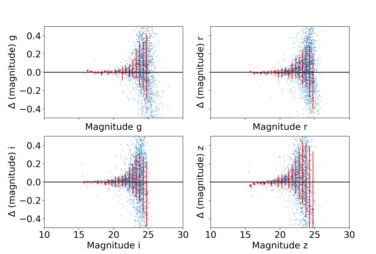
Figure 1: Example of the difference between magnitudes measured by DES and high-z clusters, in each used filter for stars detected in the field of the cluster SPT-CLJ0310-4647, located at $z=0.710$ after the SLR correction. The red dots is the average difference between those MAG$\_$AUTO and the error bars correspond to the standard deviation of the differences.

As we mentioned, we have two sets of data. The first comes from the DES DR2 database public repository, and the second, with deeper photometry, comes from our own reductions. Following the catalogues calibration described in the preceding section, hereafter we will create the final sample joining both catalogues in the following way: 65 clusters from DES described in Table 5 at $0.1<z<0.65$ (henceforth the DES clusters sample), and the 19 clusters from DeROSITAS at redshift higher than 0.65 (henceforth the high-z clusters sample) detailed in Table 4. As those two catalogues were obtained from two different pipelines, we expect slight differences. To reduce such photometric differences we correct the colour of both catalogs using the Stellar-Locus-Regression (SLR) technique High et al. (2009). Once the colour is corrected we adjust the zeropoint by adopting the DES zeropoint for the high-z clusters catalogs. The process is outlined below:

First, we calibrated the colours $g-r$, $g-i$, $r-i$, and $i-z$ for both sets of data using the SLR code. This technique uses a region in the colour-colour diagram populated by stars (Covey et al., 2007; Željko Ivezić et al., 2007). The SLR code accurately calibrates the colours for stars and galaxies using catalogued flat-fielded images without having to measure standard stars or determining the zero-points for each pass-band. The SLR technique also corrects for differences in instrumental response, atmospheric response, and for galactic extinction.

As input, the SLR code needs magnitudes, magnitudes errors, and extinction value for every source in each passband used ($g$, $r$, $i$, $z$). The dust extinction were obtained using the Schlafly & Finkbeiner Dust (Schlafly & Finkbeiner, 2011; Schlegel et al., 1998). Colour correction was made considering objects classified as stars. The photometric catalogues include the SPREAD_MODEL parameter, which is a star-galaxy separator. Following the same criteria used by  Hennig et al. (2017), we consider as stars the sources with SPREAD_MODEL < 0.002. We clean the final sample by excluding sources with IMAFLAGS_ISO > 0 in all bands to avoid saturated objects and objects with missing data  (Morganson et al., 2018) and FLAGS $\geq$ 4, to include deblended sources but excluding sources flagged with warnings during the extraction process  (DES-Collaboration et al., 2021).

As a result of the SLR calibration, we obtained corrected colours for stars and galaxies for the DES and high-z clusters catalogs. Next, we correct the absolute magnitude of the high-z clusters catalogs by comparing its star’s magnitudes to the DES star magnitudes for the $i-$band. We used a 0.25 arcseconds to match stars and a 0.5 magnitude difference to avoid variable stars. Once such correction is found (which has an average value of $\sim$ 0.02 magnitude), we applied the correction to all objects in the high-z clusters catalog.

As an example of the results of the calibration process, in Figure 1 we present four diagrams, one for each band ($g$, $r$, $i$, $z$) for the catalogues corresponding to the cluster SPTCLJ0310-4647. In those diagrams, each point corresponds to a Milky-Way star detected in the field of view of the cluster, present in both DES and DeROSITAS catalogues. Stars were selected by SPREAD_MODEL < 0.02). In the x-axis, we show the magnitude (MAG$\_$ AUTO) corresponding to the DES catalogue (taken as a base to calibrate the high-redshift data set),meanwhile in the y-axis we have the $\Delta(magnitude)$ defined as the difference between DES and high-z clusters MAG$\_$AUTO. Similar plots were obtained for the 19 clusters in common. We can see that the differences in magnitude for DES and high-z clusters observations are close to zero for the brightest end. The maximum mean difference for the brightest stars (mag < 20.5), between the two catalogues, computed as the average difference between the DES and DeROSITAS magnitudes, is around 0.04 mag in all four bands. This result suggests that the fluxes obtained using both pipelines are very close to each other and, thus, we can consider them as equivalents.

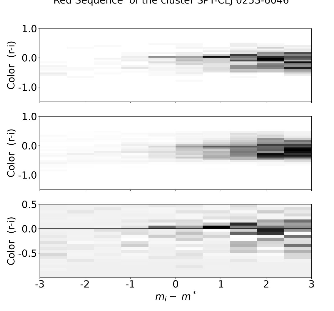
Figure 2: Background correction process for the cluster SPT-CLJ0253-6046. On the top panel, we have the detected objects inside the virial radius $R_{200}$. In the middle panel, the objects found in the background, located in the annulus between $1.5-3R_{200}$. Finally, in the bottom panel, the Red Sequence of the cluster computed as the overdensity corrected by the background. The three panels were plotted after performing the redshift slope correction for the RS time evolution. The used bins for the CMDs have a size of 0.6 in magnitude and 0.06 in colour.

4 RESULTS

The goal of this paper is to study the differences in the cluster RS galaxy population as a function of the cluster dynamical state. A galaxy spectrum is mostly flat and is mainly composed of a combination of blackbody emitters, but there is a noticeable break at 4,000 Å in the rest frame where there is an absorption of high energy radiation in the stellar atmospheres in metal poor populations (Mihalas, 1967a, b; Poggianti & Barbaro, 1997). This break allows to separate blue from red galaxies (Poggianti & Barbaro, 1997). For this reason, we used two photometric bands that contain the Balmer break in the rest frame. In those filters, the elliptical galaxies tend at a given redshift range, tend to be redder than normal galaxies at any lower redshift, thus becoming easily noticeable from the background (Gladders & Yee, 2000). Then, the selected bands depend on the redshift of each cluster, and are presented in the Table 1.

Table 1: Bands used for the colour- magnitude diagram depending on the cluster redshift to capture the 4000 Å Balmer break.

Redshift	color bands	magnitude band
$0<z\leq 0.33$	(g-r)	r
$0.33<z\leq 0.74$	(r-i)	i
$0.74<z\leq 0.9$	(i-z)	z

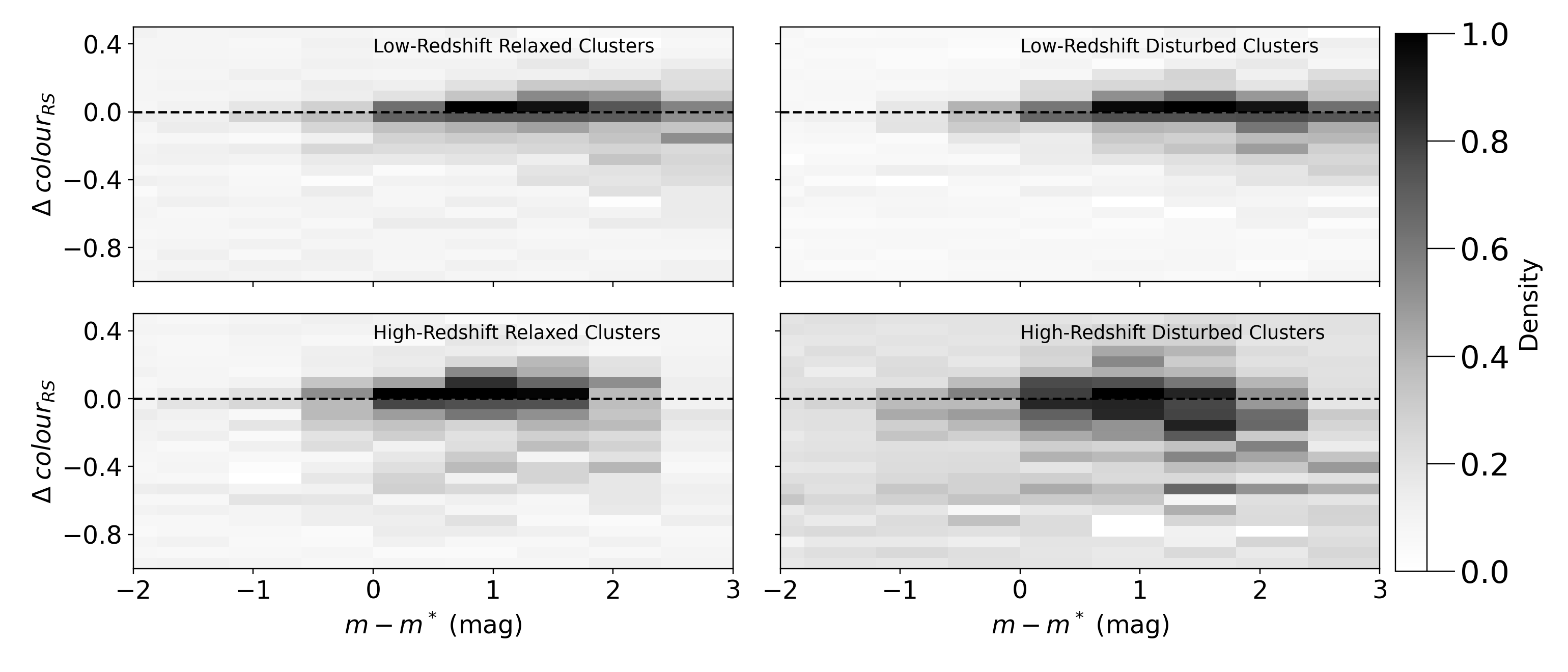
Figure 3: Colour magnitude diagram of galaxies for each studied clusters subsets. In the top row we have the low -redshift $(z<0.55)$ relaxed (left) and disturbed clusters (right) and in the bottom row we have the relaxed (left) and disturbed (right) clusters for the high redshift bins $(z>0.55)$.

Table 2: Number of clusters in the used sample in each analyzed group. We divided the sample between low and high redshift samples and relaxed and disturbed clusters.

Redshift range	Relaxed clusters	Disturbed clusters
$0.1<z<0.55$	16	27
$0.55\leq z<0.9$	25	16

To construct a cluster colour-magnitude diagram (CMD), we consider galaxies within $R_{200}$ as cluster galaxies and galaxies in the annulus between $1.5\times R_{200}<r<3\times R_{200}$ as background. Where $R_{200}$ is defined as the radius where the cluster density is 200 times the critical density of the Universe at a given redshift. The cluster centers corresponds to the SPT-SZ centers (Bleem et al., 2015), and the $R_{200}$ were estimated by Zenteno et al. (2020) using the estimated $M_{500}$, and the Duffy mass-concentration relation (Duffy et al., 2008). We bin both the cluster and background CMDs, using bins of 0.6 in magnitude and 0.06 in colour, and perform a statistical background subtraction to correct for contamination due to the projection effects.

Once the background-subtracted CMD is built for each cluster, we use a stellar population synthesis models to stack them. We do this by using models with an exponential starburst decay and a Chabrier IMF (Bruzual & Charlot, 2003) for six metallicities described in Song et al. (e.g., 2012), and Zenteno et al. (2016). Using the cluster’s redshift, and following the procedure as described by Hennig et al. (2017), we obtain the model (expected) cluster RS slope as a function of the magnitude and then subtract it from the observed slope, bringing the cluster’s colour slope to zero. The model also provides the characteristic magnitude defining the knee of the luminosity function, $m^{*}$, for each filter and redshift. The cluster redshift used in this paper corresponds to the same as Zenteno et al. (2020), which are photometric and spectroscopic redshifts collected from several literature sources.
In Figure 2, we show the process of the background correction for the SPT-CLJ0253-6046 galaxy cluster, located at $z=0.45$. For this cluster we used the $r$ and $i$ bands. In the horizontal axis we have the magnitude ($m_{i}-m^{*}$), with $m^{*}$ obtained from the model. The three vertical axes show the $r-i$ colour. In the top panel, we show the density of objects within the virial radius, plotted in gray scale. The middle panel focuses on objects located between $1.5$ to $3$ viral radius. Finally, in the bottom panel we show the resulting red sequence, obtained after subtracting the number object in the background from the number of objects within $R_{200}$, normalized by their areas.

We then combined the cluster CMDs by adding all background-corrected numbers of galaxies, normalised by the total number of clusters used in each bin. De Propris et al. (2016) studied the evolution of galaxies as they experience gravitational infall into cluster cores during merging processes, resulting in a transformation of the cluster RS (red sequence) morphology, as previously observed by De Lucia et al. (2007); Stott et al. (2007). The RS evolution below $z\sim 0.5-0.6$ shows that there are little or no morphological changes in the galaxy population, unlike earlier in time. For this reason, we separated the cluster sample in two redshift bins: the first one includes clusters between $0.1<z<0.55$ (low redshift bin), and the second one includes clusters with redshifts between $0.55\leq z<0.9$. Additionally, we subdivided our cluster sample according to their dynamic state. As a result, we have four subgroups of clusters: disturbed and relaxed clusters at low and high redshifts. The number of clusters in each subgroup is presented in Table 2. It should be noticed that we have at least 16 clusters in each subgroup.

The dynamical state of the clusters used in this paper was estimated by (Zenteno et al., 2020). They classified between relaxed and disturbed clusters using four different proxies: The offset between the position of the BCG and the SZ centroid ($D_{BCG-SZ}$), the core temperature, the morphological parameter($A_{Phot}$), which measures the asymmetry of the X-ray emission, and the offset between the BCG and the peak of X-ray emission. In this analysis, a cluster is defined as relaxed if it met any of the following three conditions: i) the cluster has $A_{phot}<0.1$, ii) the cluster has a cool core $(K_{0}<30~{}\text{keV cm}^{2})$ (McDonald et al., 2013), or iii) the offset between BCG and X-ray peak is less than 42 kpc (Mann & Ebeling, 2012). Meanwhile, the clusters were classified as disturbed if the offset between the position of the BCG and the position of the SZ centroid $D_{BCG-SZ}$ is greater than 0.4 $R_{200}$. The last criterion was chosen given that the distribution of $D_{BCG-SZ}$ looks flat after this value. Clusters that don’t meet any of the four previously mentioned criteria are considered in an intermediate evolutionary state and are excluded from this analysis. The BCG position is used as a proxy of the collisionless component since it is expected to quickly fall to the lowest region of the potential well (Tremaine, 1990). This position was derived from optical observations. Meanwhile, the centroid of the SZ was used as a proxy for the collisional component. When a cluster interacts with other clusters or groups, the gas, dark matter and galaxy components act differently depending on their nature. Then, the offset between the collisional and collisionless matter components can be used as a proxy to quantify the relaxation state of clusters (Zenteno et al., 2020).

In Figure 3, we present the stacked CMD for the four subgroups: low and high redshift relaxed clusters and low and high redshift disturbed clusters. The gray scale covers the same numeric range in the four panels. Darker (lighter) colours represents higher (lower) density regions in colour-magnitude space. In all panels we see a dominant RS with an associated bluer galaxy population. For the low redshift sample, we find that disturbed and relaxed clusters red sequence show similar colour distributions. This is, the relative contribution from early- and late-type galaxy populations to the CMD is comparable in both cases, indicating that the current dynamical state of a galaxy cluster has little impact on its CMD at the present-day. On the other hand, on the bottom panels of Figure 3 we show the RS for the high redshift sample. These RS distributions are generally wider with respect to the low-redshift counterpart. More interestingly, we observe a wider colour distribution in the disturbed cluster population when compared with both the high redshift relaxed distribution and the overall low redshift sample.

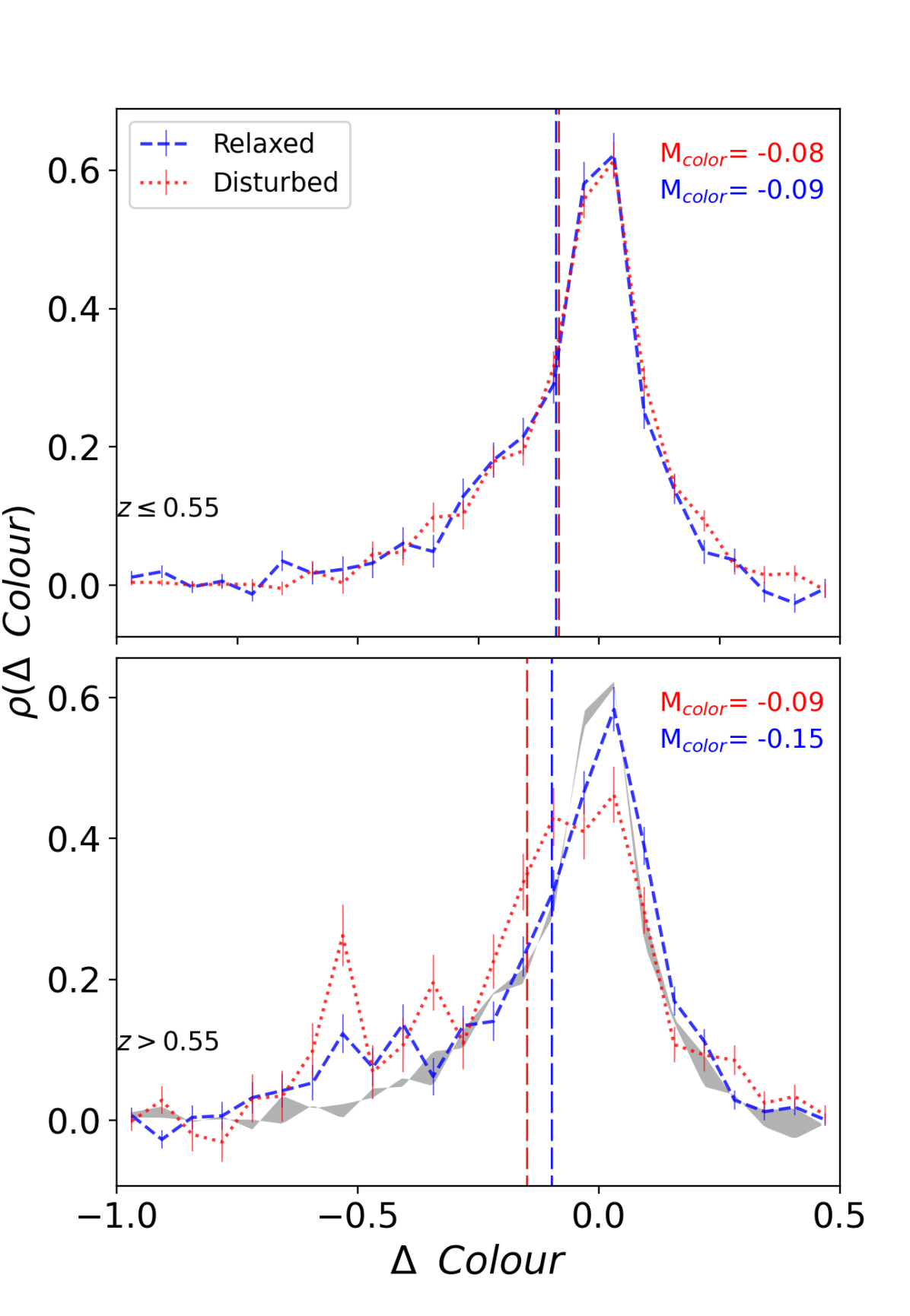
Figure 4: Colour density distributions for galaxies in each sample bin. The top panel presents the colour density distribution for the low-redshift bins relaxed in the blue line and disturbed in the red line and their error bars were computed as a Poisson noise. The vertical dashed lines indicate the median of the corresponding distribution. The bottom panel presents the same as described before, but for the high redshift $(z>0.55)$ clusters, also in gray scale we show the density distribution for the low-redshift clusters.

Figure 4 shows histograms from collapsing Figure 3 in the magnitude ($m-m^{*}$) axis for the four studied subgroups. Those histograms are normalized by their euclidean norm. In the upper panel we have the relaxed and disturbed clusters for low redshift clusters ($z<0.55$). Similarly, in the bottom panel we have the galaxy color distribution for high redshift clusters ($z>0.55$), relaxed in blue, and disturbed in red. Error bars were computed as Poisson noise. In this plot, we also present in vertical dashed lines the medians of the color distribution, we can see that for the low-redshift sample, the color density distribution is very similar for the relaxed and disturbed clusters, and the medians are also nearly identical. However, in the bottom panel, we can see an excess of blue galaxies in the disturbed sample compared to the relaxed clusters. The differences showed in the bottom panel are above the observational uncertainties, and the values of the medians are significantly different, -0.09 for relaxed, and -0.15 for disturbed clusters. This result shows that the galaxy population of disturbed clusters is bluer and possibly less quenched compared to the relaxed clusters.

5 Discussion and Conclusions

We used optical data for 84 galaxy clusters detected by SPT-SZ and optically confirmed by the DES survey. The data set is composed by 65 galaxy clusters from DES survey DR2 and 19 high-z clusters from our dedicated observations. Both data sets were observed using the Blanco telescope and the Dark Energy Camera. In order to have an homogeneous data set, we performed a calibration using the Stellar Locus Regression code. This allowed us to correct systematic differences between both data sets. We divided the final sample in two redshift bins at $z=0.55$. The results summarized in Fig. 4, show that, as expected, high redshift clusters have a more significant blue galaxy population with respect to the low redshift subsample (see e.g. Butcher & Oemler, 1984). At $z\lesssim 0.55$ the relaxed and disturbed show almost identical CMDs. However, at $z\gtrsim 0.55$ we see significant differences in their cluster galaxy colour distribution. Specifically, the disturbed sample shows an excess of blue galaxies with respect to the relaxed sample.

This result provides more evidence that the galaxy colour distribution not only depends strongly on the global environment (e.g. Peng et al., 2010; Iovino, A. et al., 2010; Muzzin et al., 2012), but also depends on the dynamical state of the clusters (e.g., Stroe et al., 2017; Zenteno et al., 2020; Stroe & Sobral, 2021), at least at $z\gtrsim 0.55$. Our results are consistent with the anti-correlation between the relaxed state of the cluster and their star formation activity found by Cohen et al. (2015) and Hou et al. (2012). The two possible explanations for the excess in the blue population are the same than the ones proposed by Cohen et al. (2015) for the enhancement of the SFR: i) the merging process triggers star formation in the galaxies inside the merging clusters generating a more mixed and bluer galaxy population or ii) disturbed clusters correspond to a less evolved state than relaxed clusters. Its worth noting that our results are consistent with Pallero et al. (2019). Using a suite of fully cosmological hydrodynamical simulations, they showed that most quenched galaxies in massive halos ($M_{200}>10^{14}M_{\odot}$) at $z<0.5$ were quenched in ex-situ groups or clusters. However for $z>0.5$ the in-situ quenched galaxies dominates their population, suggesting that the galaxies quenched inside the first cluster they fall in. In this scenario, at $z>0.5$ relaxed clusters would have a redder population than disturbed clusters, as they have had more time to evolve their population in-situ. At $z<0.5$ that difference disappears; the disturbed sample and relaxed clusters have the same galaxy population since they are being assembled from structures whose members have been already preprocessed within massive substructures. Indeed, this scenario could explain why the galaxy colour distribution at low redshift is the same in both, relaxed and disturbed sample. It is worth to mention that our results do not change if SLR correction is not applied to the data in §3.

Based on the results obtained in this paper, it is not possible to conclude what is the physical mechanism driving the excess of blue galaxies in disturbed high-z clusters. In a follow-up article, we will compare our results against cosmological simulations to characterise the mechanisms responsible for such differences.

Data Availability

The Dark Energy Survey data underlying this article are available at https://www.darkenergysurvey.org/the-des-project/data-access/

Appendix A Bands Mixture Analysis

In this section, we analyze the effect of mixing photometric bands during the construction of the cluster RS. As showed in Table 3, we join in the low redshift bin clusters observed with $g-r$ $(z\leq 0.33)$ filters and $r-i$ $(0.33<z\leq 0.55)$ filters and for the high redshift bin, we join $r-i$ $(0.55<z\leq 0.74)$ and $i-z$ $(0.74<z\leq 0.9)$ observations. Those bands capture the 4000 Å Balmer break that allows us to detect a prominent cluster Red Sequence. The RS position in the CMD was corrected using the Bruzual & Charlot (2003) stellar evolution model before stacking to avoid introducing a redshift bias in our sample. However, in this section we repeated the analysis using just the clusters observed between $0.33<z\leq 0.74$ using $r-i$ bands to confirm that the differences observed between relaxed and disturbed clusters for high redshift bin is not a consequence of mixing photometric bands. In Table 3, we have the number of stacked clusters for each considered subgroups, we can see that in each subgroup we have at least 12 clusters for low redshift bins and 22 clusters for high redshift bins.

Table 3: Number of cluster in low and redshift bins considering the clusters observed using just the $r$ and $i$ bands.

Redshift range	Relaxed clusters	Disturbed clusters
$0.33<z<0.55$	12	22
$0.55\leq z<0.74$	19	15

Similar to the previous analysis, we stacked the CMD in each subgroup after the redshift correction using the Bruzual & Charlot (2003) stellar evolution model. The morphology of the RS is the same that the showed in the Fig. 3 and the conclusions are the same: at low redshift bins, the galaxy population is mainly dominated by early-type galaxies, however at high redshift bins, there is a remnant blue (no yet-quenched) galaxy population.

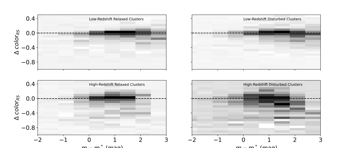
Figure 5: Similar to Fig. 3 but using only the r-i vs i colour magnitude diagram. In the top row we have the low$-z$ $(0.33<z<0.55)$ relaxed (left) and disturbed clusters (right), and in the bottom row we have the relaxed (left) and disturbed (right) clusters for the high$-z$ bin $(0.55<z<0.74)$. It can be seen that combining multiple colours do not affect our results.

We also repeated a colour density diagram presented in the Fig. 4 for cluster observed with $r-i$ bands presenting in the Fig. 6. We can see that those diagrams are very similar and the differences in colour are maintained between relaxed and disturbed clusters at high redshift bins. We also can conclude that the galaxy population at high redshift bins is more mixed in disturbed clusters compared to relaxed ones. With those two plots, we showed that the morphological differences in the RS come from the intrinsic properties of clusters and not from the bands mixing process.

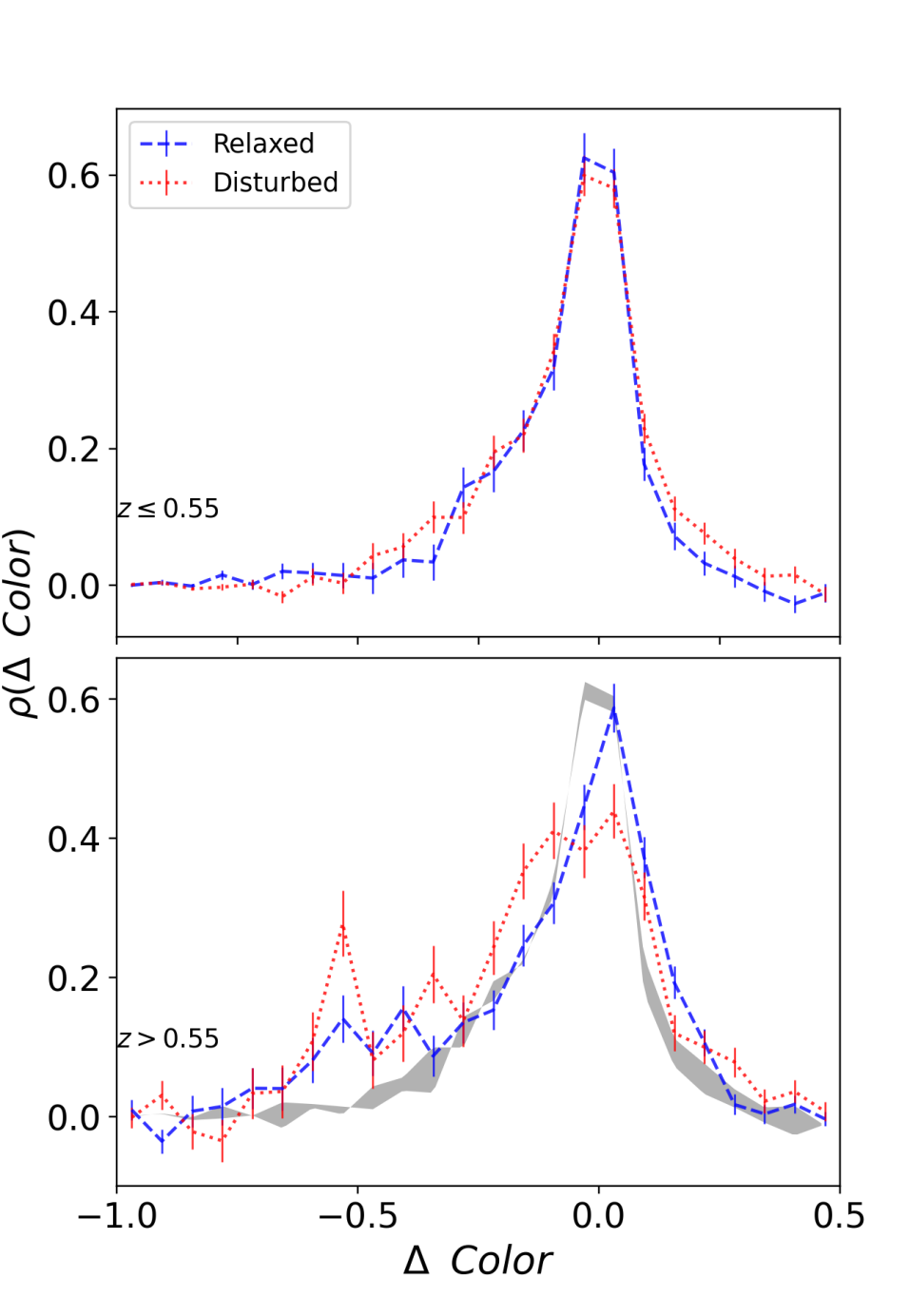
Figure 6: Similar to Fig. 4 but using only the r-i vs i colour magnitude diagram. The top panel presents the colour density distribution for the low -redshift bins relaxed in blue line and disturbed in red. Bottom panel the same for $(z>0.55)$. It can be seen that combining multiple colours do not affect our results.

Appendix B List of clusters

In Table 4, we present the list of the 19 high-redshift clusters observed in the frame of the DeROSITAS survey. Alongside their names, we also present the redshift, virial mass (SZ-based), and virial radius obtained using spectroscopic and photometric observations as specified in (Zenteno et al., 2020). In Table 5, we present the list of the clusters observed by DES including their redshifts, masses and radius. Finally, in Table 6, we present the exposure time, FWHM and the number of observations made for one of those 19 high-z galaxy clusters in bands ($r$, $i$, and, $z$). .

Name	SPT RA	SPT Dec.	$z$	$M_{200}$	$R_{200}$
SPT-CL	J2000	J2000		$10^{14}h^{-1}_{70}\;M_{\odot}$	$\arcmin$
J0014-4952	3.69	-49.87	0.752	3.27	8.10
J0058-6145	14.58	-61.76	0.83	2.87	6.65
J0131-5604	22.93	-56.08	0.69	3.17	6.17
J0230-6028	37.64	-60.46	0.68	3.06	5.41
J0310-4647	47.62	-46.78	0.709	3.17	6.53
J0313-5645	48.26	-56.75	0.66	2.82	3.96
J0324-6236	51.05	-62.60	0.75	3.21	7.57
J0406-4805	61.72	-48.08	0.737	3.16	7.01
J0406-5455	61.69	-54.92	0.74	2.86	5.23
J0422-4608	65.74	-46.14	0.7	2.79	4.36
J0441-4855	70.45	-48.91	0.79	3.05	7.23
J0528-5300	82.02	-53.00	0.768	2.84	5.53
J0533-5005	83.40	-50.09	0.881	2.64	5.78
J2043-5035	310.82	-50.59	0.723	3.18	6.88
J2222-4834	335.71	-48.57	0.652	3.62	8.22
J2228-5828	337.21	-58.46	0.71	2.85	4.77
J2242-4435	340.51	-44.58	0.73	2.66	4.10
J2259-6057	344.75	-60.95	0.75	3.34	8.57
J2352-4657	358.06	-46.95	0.73	3.14	6.71

Table 4: 19 high-z clusters used in this analysis. The redshift, virial mass and virial radius were obtained from Zenteno et al. (2020)

.

Name	SPT RA	SPT Dec.	$z$	$M_{200}$	$R_{200}$
SPT-CL	J2000	J2000		$10^{14}h^{-1}_{70}\;M_{\odot}$	$\arcmin$
J0000-5748	0.24	-57.80	0.702	3.25	6.91
J0033-6326	8.47	-63.44	0.597	3.67	7.12
J0038-5244	9.72	-52.74	0.42	4.16	4.79
J0107-4855	16.88	-48.91	0.6	3.08	4.24
J0111-5518	17.84	-55.31	0.56	3.23	4.23
J0123-4821	20.79	-48.35	0.655	3.38	6.73
J0135-5904	23.97	-59.08	0.49	3.57	4.28
J0144-4807	26.17	-48.12	0.31	5.27	4.8
J0145-5301	26.26	-53.02	0.117	14.25	7.73
J0147-5622	26.96	-56.37	0.64	3.01	4.54
J0151-5654	27.78	-56.91	0.29	5.54	4.75
J0152-5303	28.23	-53.05	0.55	3.79	6.59
J0200-4852	30.14	-48.87	0.498	4.18	7.13
J0212-4657	33.10	-46.95	0.655	3.71	8.93
J0217-4310	34.41	-43.18	0.52	3.89	6.3
J0231-5403	37.77	-54.05	0.59	3.26	4.87
J0232-5257	38.18	-52.95	0.556	4.03	8.08
J0243-5930	40.86	-59.51	0.635	3.48	6.92
J0253-6046	43.46	-60.77	0.45	3.9	4.6
J0256-5617	44.09	-56.29	0.58	3.7	6.83
J0257-4817	44.44	-48.29	0.46	3.93	4.95
J0257-5732	44.35	-57.54	0.434	4.04	4.73
J0257-5842	44.39	-58.71	0.44	4.09	5.05
J0304-4748	46.15	-47.81	0.51	3.93	6.2
J0307-5042	46.95	-50.70	0.55	4.03	7.92
J0307-6225	46.83	-62.43	0.579	3.84	7.63
J0317-5935	49.32	-59.58	0.469	4.12	5.96
J0334-4659	53.54	-46.99	0.485	4.48	8.29
J0337-4928	54.45	-49.47	0.53	3.59	5.14
J0337-6300	54.46	-63.01	0.48	3.77	4.81
J0342-5354	55.52	-53.91	0.53	3.58	5.11
J0343-5518	55.76	-55.30	0.55	3.59	5.61
J0352-5647	58.23	-56.76	0.649	3.34	6.41
J0354-5904	58.56	-59.07	0.41	4.61	6.19
J0403-5719	60.96	-57.32	0.466	4.05	5.58
J0429-5233	67.43	-52.56	0.53	3.32	4.08
J0439-4600	69.80	-46.01	0.34	5.77	7.86
J0439-5330	69.92	-53.50	0.43	4.23	5.32
J0451-4952	72.96	-49.87	0.39	4.34	4.6
J0509-5342	77.33	-53.70	0.461	4.52	7.57
J0522-5026	80.51	-50.43	0.52	3.51	4.62
J0526-5018	81.50	-50.31	0.58	3.15	4.25
J0542-4100	85.71	-41.00	0.642	3.6	7.82
J0550-5019	87.55	-50.32	0.65	2.9	4.17
J0551-5709	87.90	-57.15	0.423	4.79	7.42
J0559-5249	89.925	-52.82	0.609	3.88	8.76
J0600-4353	90.06	-43.88	0.36	5.4	7.35
J0611-4724	92.92	-47.41	0.49	3.9	5.56
J0612-4317	93.02	-43.29	0.54	3.73	6.02
J2011-5725	302.85	-57.42	0.279	5.88	5.16
J2022-6323	305.52	-63.39	0.383	4.85	6.17
J2040-5342	310.21	-53.71	0.55	3.66	5.94
J2055-5456	313.99	-54.93	0.139	11.8	6.99
J2130-6458	322.72	-64.97	0.316	5.96	7.25
J2134-4238	323.50	-42.64	0.196	9.45	8.85
J2140-5331	325.03	-53.51	0.56	3.31	4.56
J2146-5736	326.69	-57.61	0.602	3.36	5.57
J2148-6116	327.18	-61.27	0.571	3.71	6.7
J2232-5959	338.14	-59.99	0.594	3.89	8.39
J2233-5339	338.32	-53.65	0.44	4.81	8.23
J2254-5805	343.58	-58.08	0.153	9.75	5.08
J2331-5051	352.96	-50.86	0.576	3.99	8.46
J2332-5358	353.10	-53.96	0.402	5.08	7.89
J2344-4224	356.14	-42.41	0.29	5.44	4.49
J2358-6129	359.70	-61.48	0.37	4.92	5.92

Table 5: 65 DES clusters used in this analysis. The redshift, virial mass and virial radius were obtained from Zenteno et al. (2020)

.

Name	Exposure Timesa (s)			FWHM (”)			Nobs
	$r$	$i$	$z$	$r$	$i$	$z$	$r$	$i$	$z$
J0014-4952	–	1840	2090	–	0.95	0.78	–	10	11
J0058-6145	–	3150	4746	–	1.06	1.16	–	15	21
J0131-5604	–	1200	1800	–	0.97	0.82	–	8	10
J0230-6028	–	1200	2938	–	0.94	1.15	–	8	13
J0310-4647	–	3750	1800	–	1.03	0.90	–	27	10
J0313-5645	–	1080	3080	–	1.10	1.17	–	9	14
J0324-6236	–	2000	2640	–	1.00	0.87	–	10	15
J0406-4805	–	1575	2460	–	0.96	0.94	–	8	12
J0406-5455	–	1600	3750	–	1.01	0.88	–	8	15
J0422-4608	–	2638	2152	–	0.91	1.03	–	18	13
J0441-4855	–	1400	4200	–	0.84	0.99	–	7	14
J0528-5300	–	3000	3300	–	1.11	1.03	–	15	11
J0533-5005	–	5700	4815	–	0.98	0.86	–	19	15
J2043-5035	2045	1664	1400	1.30	1.10	0.84	14	8	7
J2222-4834	1050	1080	–	1.39	0.81	–	9	9	–
J2228-5828	600	–	–	1.51	–	–	4	–	–
J2242-4435	2085	1335	2000	1.22	1.52	0.81	15	10	10
J2259-6057	–	3579	3600	–	1.13	1.01	–	18	18
J2352-4657	–	1582	5350	–	0.97	0.89	–	9	22

Table 6: Observations of the high-z clusters sample. ^aThe exposure times shown are in addition to the observations carried out by DES (Abbott et al., 2021), which were included in the final $griz$ stacks.

References

- Abbott et al. (2021) Abbott T. M. C., et al., 2021, ApJS, 255, 20
- Abell (1954) Abell G. O., 1954, ApJS, 3, 211
- Andrade-Santos et al. (2017) Andrade-Santos F., et al., 2017, ApJ, 843, 76
- Bauer et al. (2005) Bauer F. E., Fabian A. C., Sanders J. S., Allen S. W., Johnstone R. M., 2005, MNRAS, 359, 1481
- Bertin (2011) Bertin E., 2011, Analysis, 442, 435
- Bertin & Arnouts (1996) Bertin E., Arnouts S., 1996, A&AS, 117, 393
- Bleem et al. (2015) Bleem L. E., Stalder B., Haan T. D., 2015, ApJS, 216
- Bleem et al. (2020) Bleem L. E., et al., 2020, ApJS, 247, 25
- Bower et al. (1992) Bower R. G., Lucey J. R., Ellis R. S., 1992, MNRAS, 254, 601
- Brodwin et al. (2013) Brodwin M., et al., 2013, ApJ, 779, 138
- Bruzual & Charlot (2003) Bruzual G., Charlot S., 2003, MNRAS, 344, 1000
- Butcher & Oemler (1984) Butcher H., Oemler A. J., 1984, ApJ, 285, 426
- Cassano et al. (2010) Cassano Brunetti, G. Röttgering, H. J. A. Brüggen, M. 2010, A&A, 509, A68
- Cohen et al. (2015) Cohen S. A., Hickox R. C., Wegner G. A., 2015, ApJ, 806, 85
- Connor et al. (2019) Connor T., Kelson D. D., Donahue M., Moustakas J., 2019, ApJ, 875, 16
- Covey et al. (2007) Covey K. R., et al., 2007, AJ, 134, 2398
- DES-Collaboration et al. (2021) DES-Collaboration et al., 2021, ApJS, 255, 20
- De Lucia et al. (2007) De Lucia G., et al., 2007, MNRAS, 374, 809
- De Propris et al. (2016) De Propris R., Bremer M. N., Phillipps S., 2016, MNRAS, 461, 4517
- Desai et al. (2012) Desai S., et al., 2012, ApJ, 757, 83
- Dressler (1980) Dressler A., 1980, ApJ, 236, 351
- Dressler & Shectman (1988) Dressler A., Shectman S. A., 1988, AJ, 95, 985
- Drlica-Wagner et al. (2021) Drlica-Wagner A., et al., 2021, ApJS, 256, 2
- Duffy et al. (2008) Duffy A. R., Schaye J., Kay S. T., Dalla Vecchia C., 2008, MNRAS, 390, L64
- Evans et al. (2018) Evans D. W., et al., 2018, A&A, 616, A4
- Ferrari et al. (2003) Ferrari C., Maurogordato, S. Cappi, A. Benoist, C. 2003, A&A, 399, 813
- Flaugher et al. (2015) Flaugher B., et al., 2015, AJ, 150
- George et al. (2020) George K., Vassallo T., Mohr J., Mirkazemi M., Israel H., de Jong J. T. A., Verdoes Kleijn G. A., 2020, in Pizzo R., Deul E. R., Mol J. D., de Plaa J., Verkouter H., eds, ASPCS Vol. 527, Astronomical Data Analysis Software and Systems XXIX. p. 701
- Gladders & Yee (2000) Gladders M. D., Yee H. K. C., 2000, AJ, 120, 2148
- Gladders & Yee (2005) Gladders M. D., Yee H. K. C., 2005, ApJS, 157, 1
- Gladders et al. (2007) Gladders M. D., Yee H. K. C., Majumdar S., Barrientos L. F., Hoekstra H., Hall P. B., Infante L., 2007, ApJ, 655, 128
- H. Neilsen et al. (2016) H. Neilsen J., Bernstein G., Gruendl R., Kent S., 2016, doi:10.2172/1250877
- Hennig et al. (2017) Hennig C., et al., 2017, MNRAS, 467, 4015
- High et al. (2009) High F. W., Stubbs C. W., Rest A., Stalder B., Challis P., 2009, AJ, 138, 110
- Hilton et al. (2009) Hilton M., et al., 2009, ApJ, 697, 436
- Hou et al. (2012) Hou A., et al., 2012, MNRAS, 421, 3594
- Hubble & Humason (1931) Hubble E., Humason M. L., 1931, ApJ, 74, 43
- Iovino, A. et al. (2010) Iovino, A. et al., 2010, A&A, 509, A40
- Jaffé et al. (2011) Jaffé Y. L., Aragón-Salamanca A., De Lucia G., Jablonka P., Rudnick G., Saglia R., Zaritsky D., 2011, MNRAS, 410, 280
- Klein et al. (2017) Klein M., et al., 2017, MNRAS, 474, 3324
- Klein et al. (2019) Klein M., et al., 2019, MNRAS, 488, 739
- Kleiner et al. (2014) Kleiner D., Pimbblet K. A., Owers M. S., Jones D. H., Stephenson A. P., 2014, MNRAS, 439, 2755
- Kodama & Arimoto (1997) Kodama T., Arimoto N., 1997, A&A, 320, 41
- Komatsu et al. (2011) Komatsu E., et al., 2011, ApJS, 192, 18
- Kravtsov & Borgani (2012) Kravtsov A. V., Borgani S., 2012, ARA&A, 50, 353
- Kron (1980) Kron R. G., 1980, ApJS, 43, 305
- Mancone et al. (2010) Mancone C. L., Gonzalez A. H., Brodwin M., Stanford S. A., Eisenhardt P. R. M., Stern D., Jones C., 2010, ApJ, 720, 284
- Mann & Ebeling (2012) Mann A. W., Ebeling H., 2012, MNRAS, 420, 2120
- McDonald et al. (2013) McDonald M., et al., 2013, ApJ, 774, 23
- Merloni et al. (2012) Merloni A., et al., 2012, arXiv e-prints, p. arXiv:1209.3114
- Mihalas (1967a) Mihalas D., 1967a, ApJ, 149, 169
- Mihalas (1967b) Mihalas D., 1967b, ApJ, 150, 1168
- Morganson et al. (2018) Morganson E., et al., 2018, PASP, 130, 1
- Murphy et al. (2012) Murphy D. N. A., Geach J. E., Bower R. G., 2012, MNRAS, 420, 1861
- Muzzin et al. (2012) Muzzin A., et al., 2012, ApJ, 746, 188
- Oemler (1974) Oemler Augustus J., 1974, ApJ, 194, 1
- Owers et al. (2012) Owers M. S., Couch W. J., Nulsen P. E. J., Randall S. W., 2012, ApJ, 750, L23
- Pallero et al. (2019) Pallero D., Gó mez F. A., Padilla N. D., Torres-Flores S., Demarco R., Cerulo P., Olave-Rojas D., 2019, MNRAS, 488, 847
- Papovich et al. (2010) Papovich C., et al., 2010, ApJ, 716, 1503
- Peng et al. (2010) Peng C. Y., Ho L. C., Impey C. D., Rix H. W., 2010, AJ, 139, 2097
- Poggianti & Barbaro (1997) Poggianti B. M., Barbaro G., 1997, å, 325, 1025
- Pranger et al. (2014) Pranger F., et al., 2014, A&A, 567, C1
- Rykoff et al. (2016) Rykoff E. S., et al., 2016, ApJS, 224, 1
- Santos et al. (2008) Santos J. S., Rosati P., Tozzi P., Böhringer H., Ettori S., Bignamini A., 2008, A&A, 483, 35
- Sarazin (2002) Sarazin C. L., 2002, The Physics of Cluster Mergers. Springer Netherlands, Dordrecht, pp 1–38, doi:10.1007/0-306-48096-4_1
- Sarazin (2004) Sarazin C. L., 2004, Journal of Korean Astronomical Society, 37, 433
- Schlafly & Finkbeiner (2011) Schlafly E. F., Finkbeiner D. P., 2011, ApJ, 737
- Schlegel et al. (1998) Schlegel D. J., Finkbeiner D. P., Davis M., 1998, ApJ, 500, 525
- Shim et al. (2011) Shim H., et al., 2011, ApJ, 727
- Snyder et al. (2012) Snyder G. F., et al., 2012, ApJ, 756, 114
- Sobral et al. (2015) Sobral D., Stroe A., Dawson W. A., Wittman D., Jee M. J., Röttgering H., van Weeren R. J., Brüggen M., 2015, MNRAS, 450, 630
- Song et al. (2012) Song J., et al., 2012, ApJ, 761
- Stanford et al. (1998) Stanford S. A., Eisenhardt P. R., Dickinson M., 1998, ApJ, 492, 461
- Stott et al. (2007) Stott J. P., Smail I., Edge A. C., Ebeling H., Smith G. P., Kneib J.-P., Pimbblet K. A., 2007, ApJ, 661, 95
- Stroe & Sobral (2021) Stroe A., Sobral D., 2021, ApJ, 912, 55
- Stroe et al. (2017) Stroe A., Sobral D., Paulino-Afonso A., Alegre L., Calhau J., Santos S., van Weeren R., 2017, MNRAS, 465, 2916
- Tremaine (1990) Tremaine S., 1990, in Wielen R., ed., Dynamics and Interactions of Galaxies. Springer Berlin Heidelberg, Berlin, Heidelberg, pp 394–405
- Vakili et al. (2020) Vakili M., et al., 2020, arXiv
- Visvanathan & Sandage (1977) Visvanathan N., Sandage A., 1977, ApJ, 216, 214
- Voit (2005) Voit G. M., 2005, Reviews of Modern Physics, 77, 207
- Yoon & Im (2020) Yoon Y., Im M., 2020, ApJ, 893, 117
- Yuan et al. (2022) Yuan Z. S., Han J. L., Wen Z. L., 2022, MNRAS, 513, 3013
- Zenteno et al. (2016) Zenteno A., et al., 2016, MNRAS, 462, 830
- Zenteno et al. (2020) Zenteno A., et al., 2020, MNRAS, 495, 705
- Zhang et al. (2009) Zhang Y.-Y., Reiprich T. H., Finoguenov A., Hudson D. S., Sarazin C. L., 2009, ApJ, 699, 1178
- Zhang et al. (2022) Zhang B., Cui W., Wang Y., Dave R., De Petris M., 2022, MNRAS, 516, 26
- Željko Ivezić et al. (2007) Željko Ivezić et al., 2007, AJ, 134, 973