Towards Quantifying the Impact of Triaxiality on Optical Signatures of Galaxy Clusters: Weak Lensing and Galaxy Distributions

Abstract

We present observational evidence of the impact of triaxiality on radial profiles that extend to 40 Mpc from galaxy cluster centres in optical measurements. We perform a stacked profile analysis from a sample of thousands of nearly relaxed galaxy clusters from public data releases of the Dark Energy Survey (DES) and the Dark Energy Camera Legacy Survey (DECaLS). Using the central galaxy elliptical orientation angle as a proxy for galaxy cluster orientation, we measure cluster weak lensing and excess galaxy density axis-aligned profiles, extracted along the central galaxy’s major or minor axes on the plane-of-the-sky. Our measurements show a $\gtrsim 2-3\sigma$ difference per radial bin between the normalized axis-aligned profiles. The profile difference between each axis-aligned profile and the azimuthally averaged profile ($\sim\pm 10-20\%$ along major/minor axis) appears inside the clusters ($\sim 0.4$ Mpc) and extends to the large-scale structure regime ($\sim 10-20$ Mpc). The magnitude of the difference appears to be relatively insensitive to cluster richness and redshift, and extends further out in the weak lensing surface mass density than in the galaxy overdensity. Looking forward, this measurement can easily be applied to other observational or simulation datasets and can inform the systematics in cluster mass modeling related to triaxiality. We expect imminent upcoming wide-area deep surveys, such as the Vera C. Rubin Observatory’s Legacy Survey of Space and Time (LSST), to improve our quantification of optical signatures of cluster triaxiality.

1 Introduction

Galaxy clusters are the most massive gravitationally collapsed structures in our universe, providing both a probe for cosmology and a unique environment for galaxy formation (Allen et al., 2011; Kravtsov & Borgani, 2012). Clusters form late in cosmic history; both relatively smooth mass accretion and mergers of galaxies and groups govern the mass growth. Each galaxy cluster’s mass accretion history, in turn, depends on the large scale structure and environment in which it resides. The abundance and evolution of galaxy clusters is sensitive to the nature of dark energy (Vikhlinin et al., 2009). But, one of the primary roadblocks to cluster-based cosmology lies in our ability to precisely and accurately meausure cluster masses. With the advent of stage-4 cosmology surveys (Dodelson et al., 2016), the community is well-poised to utilize multi-wavelength information and Bayesian approaches towards improved precision and accuracy (Mulroy et al., 2019). In fact, the weak gravitational lensing observable from optical surveys is now a standard for calibrating ‘observable-mass’ relations (Mantz et al., 2015a; Bocquet et al., 2019).

While most mass estimates that use galaxy cluster mass proxies assume azimuthally symmetric signatures and on-average spherical distribution, the underlying matter distribution of galaxy clusters more closely follow a triaxial shape (Kasun & Evrard, 2005; Knebe & Wießner, 2006; Despali et al., 2014). Cluster triaxiality is one of the known systematics to weak lensing mass estimates (Becker & Kravtsov, 2011; Herbonnet et al., 2019; Zhang et al., 2023). Galaxy clusters whose major axis aligns with our line of sight will have boosted lensing signatures and systematically higher inferred masses, while those whose minor axis aligns with our line of sight will have suppressed lensing signatures (Osato et al., 2018; Herbonnet et al., 2022). The relative alignment of a galaxy cluster with our line of sight also affects other projected quantities, such as the measured member galaxy distribution (i.e. the cluster ‘richness’; Wu et al., 2022). As a result, the imprints of cluster triaxiality on observations are correlated, leading to a covariance between cluster observables. For example, clusters selected by an observable such as richness may also display a biased lensing signature (Noh & Cohn, 2012; Zhang & Annis, 2022; Farahi et al., 2022); cosmological studies need to account for such resulting selection effects. On the other hand, the associated impact of triaxiality on both the underlying mass and the galaxy distributions also allows for methods that constrain the angle and the ellipticity of the host dark matter halo  (Shin et al., 2018; Gonzalez et al., 2021). The triaxial shape of galaxy clusters affects other signatures of galaxy clusters, including X-ray isophotes (Rasia et al., 2013; Mantz et al., 2015b), and can trace aspects of the galaxy cluster environment, such as filament alignment (Tempel et al., 2015; Sifón et al., 2015; Gouin et al., 2020; Lokken et al., 2022).

The shape and orientation of the central galaxy (CG) or the brightest cluster galaxy (BCG) can serve as proxies that describe its host cluster triaxiality. Compared with measurements of the member galaxy distribution and lensing mass distribution, measurements of the CG are relatively less affected by noise. Additionally, CG measurements are more readily available for larger optical samples of galaxy clusters. Other proxies, such as X-ray isophotes that trace the gas morphology, require many photon counts to constrain gas shapes and are more limited in availability (e.g. Rasia et al., 2013; Mantz et al., 2015b). Similarly, the resolution of Sunyaev–Zel’dovich (SZ) effect observations hinders morphology measurements at high redshifts, but have been achieved for a small sample of clusters at relatively low redshifts (e.g. Donahue et al., 2016). Such shape observations of higher redshift clusters exist for smaller samples (e.g. Rodríguez-Gonzálvez et al., 2017; Kitayama et al., 2023). Overall, existing optical searches provide an ample balance between coverage and depth to perform studies on cluster triaxiality in a large statistical sample (Clampitt & Jain, 2016; Shin et al., 2018). CG shapes have already been used to quantify potential biases in weak lensing cluster mass estimates due to viewing angle (Herbonnet et al., 2019), and CG orientations indicate the co-evolution with the intracluster medium (Yuan & Wen, 2022). Simulations have identified measurable correlation between the CG orientation and the underlying cluster halo mass distribution (Herbonnet et al., 2022). This, and other proxies of triaxiality are often used to identify physical mechanisms that tie galaxy clusters’ observables and their mass accretion histories (Chen et al., 2019; Machado Poletti Valle et al., 2021; De Luca et al., 2021; Sereno et al., 2021; Mendoza et al., 2023; Vallés-Pérez et al., 2023). Observations have also provided concrete evidence of correlation in the alignment of various morphology measures, including that of the CG, gas, and underlying mass distribution, thereby motivating such proxies and further studies to understand correlated alignments (Donahue et al., 2016).

The goal of this paper is to observationally investigate how cluster triaxiality impacts the distribution of the density of cluster member galaxies and galaxy cluster weak lensing signatures, and how these signatures co-vary with each other on different distance scales. In this work, we use the (observed 2D-projected) orientation of the CG as a proxy for the orientation of the underlying galaxy cluster triaxial shape and as a tracer of triaxial alignments between cluster components, which is a more commonly available measurement for optical cluster samples, such as those used in this work – the recent Dark Energy Survey (DES) Y3 catalogue (Gatti et al., 2021) and the Dark Energy Spectroscopic Instrument (DESI) Legacy Image Surveys (hereafter Legacy Surveys) catalogue (Dey et al., 2019). We use the orientation angles to align our stacked measurements of cluster member galaxy distributions and weak lensing signatures and to separate these measurements along the cluster major and minor axes. We note that, our approach is complementary to the analysis done by Shin et al. (2018), where they examined the relationship between the CG, cluster member galaxy distribution, and underlying mass distribution traced by weak gravitational lensing with quadrupole measurements. We additionally discuss how the optical signatures connect the triaxial alignment and the surrounding large scale environment, motivated by the theoretical analysis done by Osato et al. (2018).

We organize the paper as follows. In Section 2, we briefly describe the theoretical underpinnings of using the weak gravitational lensing signature of galaxy clusters to trace their underlying mass distribution, which is largely triaxial. In Section 3, we describe the galaxy cluster samples and associated weak lensing shape measurement catalogues, photometric redshifts (photo-zs) and photometry that we use in this study. Section 4 lays out the results, quantifying how radial profiles of both the galaxy number density (in and around galaxy clusters) and the weak lensing signature differ when measured along the directions of CG major and minor axes. We also discuss potential effects due to richness, redshift, or red-sequence selection in our sample. Finally, we provide our discussion of the results in Section 5, including considerations surrounding robustness of our measurements, methods of CG orientation measurements, correlation between lensing signature and number density. We summarize our work and talk about possible future directions in Section 6. In the Appendix, we show some extra tests and details, and a flow chart for our pipeline.

2 Theory

The mass of a foreground galaxy cluster deflects the light from distant background galaxies via gravitational lensing. The deflection of a light source on the image plane can be described by

$$\boldsymbol{\alpha}=\boldsymbol{\theta}-\boldsymbol{\beta}~{},$$ (1)

where $\boldsymbol{\theta}$ and $\boldsymbol{\beta}$ denote the observed position and the original position of the source respectively. The deflection and the cluster surface mass distribution $\Sigma(\boldsymbol{\theta})$ are connected through a potential, so that

$$\boldsymbol{\alpha}=\nabla\phi~{}.$$ (2)

Here,

$$\phi(\boldsymbol{\theta})=\frac{1}{\pi}\int\kappa(\boldsymbol{\theta^{\prime}})\ln{|\boldsymbol{\theta}-\boldsymbol{\theta^{\prime}}|}\,\mathrm{d}^{2}\theta^{\prime}~{}.$$ (3)

The convergence $\kappa$ satisfies

$$\nabla^{2}\phi=\nabla\cdot\boldsymbol{\alpha}=2\kappa,~{}\kappa(\boldsymbol{\theta})=\frac{\Sigma(\boldsymbol{\theta})}{\Sigma_{\textrm{crit}}}~{}.$$ (4)

$\Sigma_{\textrm{crit}}$ is the critical surface mass density satisfying

$$\Sigma_{\textrm{crit}}=\frac{v_{\textrm{c}}^{2}}{4\pi G}\frac{D_{\textrm{s}}}{D_{\textrm{l}}D_{\textrm{ls}}}~{},$$ (5)

where $D_{\textrm{s}}$, $D_{\textrm{l}}$, and $D_{\textrm{ls}}$ are the angular diameter distances between the source and the observer, the lens and the observer, the lens and the source respectively; $v_{\textrm{c}}$ is the speed of light.

The differential lensing effect (the Jacobian matrix) is

$$\frac{\partial\boldsymbol{\beta}}{\partial\boldsymbol{\theta}}=\delta_{ij}-\phi_{,ij}=(1-\kappa)I-\gamma_{1}\begin{pmatrix}1&\\ &-1\end{pmatrix}-\gamma_{2}\begin{pmatrix}&1\\ 1&\end{pmatrix}~{},$$ (6)

where $i,j=1,2$ and the shear components

$$\gamma_{1}=(\phi_{,11}-\phi_{,22})/2,~{}\gamma_{2}=\phi_{,12}=\phi_{,21}~{},$$ (7)

and thus the convergence gives an isotropic magnification, while the shear produces distortions along two axes separated by 45 degrees (Narayan & Bartelmann, 1996; Bartelmann & Schneider, 2001).

Using a loop around the cluster on the image plane and 2D divergence theorem, we have

$$\iint 2\kappa\,\mathrm{d}^{2}\theta=\oint(\nabla\phi\cdot\hat{n})\,\mathrm{d}l=\int\alpha_{n}\,\mathrm{d}l~{},$$ (8)

where $\alpha_{n}$ is the projection of $\boldsymbol{\alpha}$ along the outward normal direction of the loop. Traditionally, a circular loop with radius $\theta$ is considered, then

$$\langle\gamma_{\textrm{T}}\rangle|_{\theta}=\bar{\kappa}(<\theta)-\langle\kappa\rangle|_{\theta}\equiv\Delta\kappa(\theta)~{},$$ (9)

where $\langle\cdot\rangle|_{\theta}$ is the average at that radius, $\gamma_{\textrm{T}}$ is the shear component tangential to the loop, and $\bar{\kappa}(<\theta)$ is the mean convergence inside that loop; this is true for an arbitrary $\kappa$ distribution (Schneider, 2005). $\Delta\kappa$ is the excess convergence. If we consider a circular sector (pie-shaped) loop instead, i.e. two radii that cross at the mass centre and span an angle, with a circular arc, this equation still holds for an axis-symmetric lens. Going further, for an elliptical lens, if this angle is small, or the mass distribution is nearly axis-symmetric (which is likely true for the nearly relaxed cluster sample studied in this paper), then $\alpha_{n}$ is small on the two straight lines, and the above equation still holds approximately (Figure 1).

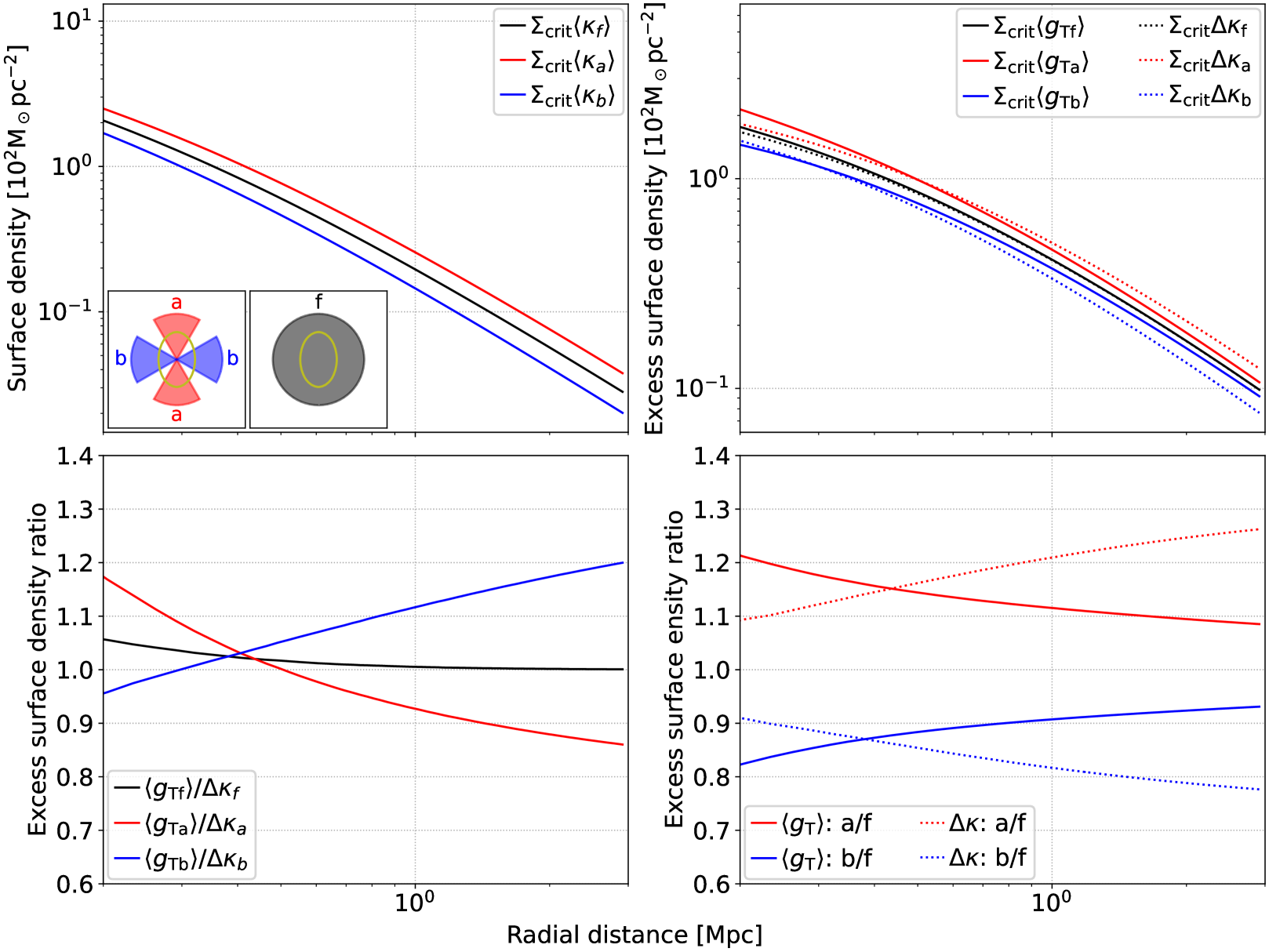
Figure 1: Example of lensing effects of an elliptical NFW cluster halo. We consider a cluster that is at redshift 0.47 and has redMaPPer richness 33 (median of the observational sample studied later in the paper; Section 3.5), and convert that to $M_{\textrm{200c}}=2\times 10^{14}M_{\odot}$, based on the DES Y1 mass-richness relation (McClintock et al., 2019) and typical $M_{\textrm{200m}}/M_{\textrm{200c}}$ ratio (Kovacs et al., 2022). The subscript 200 means the average density of the spherically enclosed overdensity mass is 200 times the critical (c) or mean matter (m) density of the universe at that redshift. We use the concentration-mass relation and cosmological parameters described by Child et al. (2018). We compute the lensing convergence and shear using the method described by Oguri (2010); Oguri et al. (2010), so that the surface density has an elliptical form $\kappa(\boldsymbol{\theta})=\kappa_{\textrm{NFW}}(\xi=\theta_{1}^{2}/q^{2}+\theta_{2}^{2})$, where NFW is the spherical profile described by Navarro et al. (1996), and $q$ is the axis ratio $b/a$ (here we select 2/3 to be consistent with our results in Section 4). We consider the radial distance range for weak lensing from 0.2 to 3 Mpc ($r_{\textrm{200c}}$ is 1 Mpc). The correlated large-scale structure (LSS; the two-halo term) is not modelled and can be aligned with the halo, and is beyond the scope of this demonstration. We select two samples ($a,b$) of areas near the major and minor axes of the ellipse ($\pm 30\deg$) and compute the respective averages along the arcs given the radial distance, and we use the azimuthal average over all position angles as a fiducial sample ($f$), similar to our strategy for processing the real data (Section 3.4). After averaging, the results are unrelated to the directions of the X-axis and Y-axis. Top left: Surface density comparison ($a>f>b$). The inset plots show the angle ranges of the three samples and the shape of the elliptical halo, which are the same in other subplots. Top right: Comparisons of excess surface density for different samples ($a>f>b$), and comparison between the reduced shear estimated excess density and the true value. Bottom left: Ratios between reduced shear and excess convergence, which shows how accurate the excess density estimate is (error $\lesssim 20\%$). Bottom right: Ratios between the major-axis sample $a$ (or the minor-axis sample $b$) and the fiducial sample ($f$) for the reduced shear and the excess density, which later we use lensing and photometry in the real observational data to study respectively (Section 4). The ratios along the two directions are nearly symmetric with respect to 1.

In the weak lensing regime, both $\kappa,~{}\boldsymbol{\gamma}\ll 1$. The lensing observable is the reduced shear

$$\boldsymbol{g}=\frac{\boldsymbol{\gamma}}{1-\kappa}~{},$$ (10)

and in weak lensing $\boldsymbol{g}\sim\boldsymbol{\gamma}$. The mean shape of background galaxies satistifies

$$\langle\boldsymbol{g}\rangle\sim\langle\boldsymbol{\gamma}\rangle\sim\langle\mathbf{\mathsf{R}}\rangle^{-1}\langle\boldsymbol{e}\rangle~{},$$ (11)

where the matrix $\mathbf{\mathsf{R}}$ is a per-object shear response (Section 3.2). The excess surface mass density $\Delta\Sigma(R)$ satisfies

$$\langle g_{\textrm{T}}\Sigma_{\textrm{crit}}\rangle|_{R}\sim\langle\gamma_{\textrm{T}}\Sigma_{\textrm{crit}}\rangle|_{R}=\overline{\Sigma}(<R)-\langle\Sigma\rangle|_{R}\equiv\Delta\Sigma(R)~{},$$ (12)

and links the lensing observable to the mass distribution within a (2D) radial distance $R$ for a circular loop. For a circular sector area (Section 3.4 and Section 4), we can similarly define an ‘effective excess surface density’ ($\widetilde{\Delta\Sigma}$) using $\langle g_{\textrm{T}}\Sigma_{\textrm{crit}}\rangle$ from a sample of background galaxies inside. Also, since the distribution of cluster galaxies approximately traces the dark matter (DM) halo, we can similarly define an excess number density, $\Delta n=\overline{n}(<R)-n(R)$, for comparison.

The lensing effect of cluster triaxiality has been studied in simulations using elliptical NFW-like models (Oguri et al., 2003). Their projected isodensity contours are concentric, aligned, and elliptical with fixed ellipticity (homoeoidal). This motivates us to consider two profiles along two perpendicular directions on the projection plane (plane of the sky) – the major and minor axes of the ellipse – where the two profiles should have the largest difference. We use their difference to detect the halo ellipticity, though the halo does not necessarily need to have an NFW shape. In addition, the profile can describe either the mass distribution, which can be observed via lensing, or the number distribution of cluster galaxies, which traces the mass distribution (Figure 2). However, the goal of this paper is not to fit the data with an elliptical model to exactly measure the ellipticity, but rather to present a simple method that can analyse the the lensing signature of cluster triaxiality without model assumption, and to study how it is related to other physical quantities. We demonstrate our method using public datasets.

Throughout the paper, we use the cosmological parameters described by Child et al. (2018) to be consistent with Figure 1 – flat $\Lambda$CDM $H_{0}=71$ km s^-1 Mpc^-1, $\Omega_{\textrm{m}}=0.2648$. We note that the physical radial distance in each cluster is the only place where the cosmological parameters get involved in this work (through the angular diameter distance); switching between commonly accepted values of the cosmological parameters only changes the distance by $\lesssim 1\%$. We use physical units rather than comoving for radial distances. The magnitudes are in the AB system (Oke & Gunn, 1983).

3 Datasets and Methods

3.1 Cluster samples

The cluster sample used in this paper is identified by the redMaPPer algorithm (Rykoff et al., 2014), which is based on searching of cluster galaxy red-sequence features in photometric datasets. The redMaPPer algorithm has been applied to a handful of galaxy catalogues including the Sloan Digital Sky Survey (SDSS) and DES, tested with multi-wavelength data from cosmic microwave background (CMB) and X-ray observations (Rozo & Rykoff, 2014; Rozo et al., 2015a) as well as spectroscopic follow-ups (Rozo et al., 2015b), and used in multiple galaxy cluster abundance cosmology studies (Costanzi et al., 2019, 2021; Abbott et al., 2020; Park et al., 2023).

We use the redMaPPer cluster catalogue derived from the DES Year 1 photometric datasets, a publicly-accessible catalogue described by McClintock et al. (2019). For each galaxy cluster in the sample, redMaPPer also identifies five CG candidates with centring probability assigned to each one (P_CEN). We use the most probable CG from this list. Because the CG orientation angle is a crucial component in this analysis, we require the clusters to have a centring probability of at least 80% associated with the most probable CG ($\max\{\texttt{P\_CEN}\}\geq 0.8$). We also use the cluster redshift information available in the catalogue (Z_LAMBDA), a photometric redshift calculation estimated from the cluster red sequence features calibrated with archival spectroscopic redshifts (spec-zs). This cluster galaxy red sequence redshift has been shown to be nearly unbiased, with a percentage level redshift scatter ($\sigma_{z}$): the median of $\sigma_{z}/(1+z)\simeq 0.006$ (McClintock et al., 2019), sufficient for this analysis. After the selection on P_CEN, the remaining 4300 clusters span richness $20<\lambda<235$ and redshift $0.2<z<0.86$. We note that the clusters that are above redshift 0.65 might have a completeness issue (McClintock et al., 2019). However, those clusters only cover a small fraction ($3\%$) and our results are not strongly sensitive to the redshift. Therefore, we still include those clusters to reduce the statistical noise.

Multi-wavelength studies of the redMaPPer clusters have provided further insight into the catalogue’s performance. X-ray (Zhang et al., 2019) and CMB (Bleem et al., 2020) studies confirmed that the most probable CGs of the redMaPPer clusters (regardless of their redMaPPer assigned centring probabilities) are correct around 75% of the time, assuring us the quality of the CG selection; the cut on P_CEN further improves the selection. In this paper, we also rely on using the richness quantity in the catalogue as a mass proxy. X-ray and weak lensing (McClintock et al., 2019) studies show that the galaxy clusters with richness above 20 correspond to a mass range of roughly $10^{14}\mathrm{M}_{\odot}h^{-1}$ and above.

Finally, to qualitatively validate the results of this paper, we also test the analysis with a cluster catalogue derived from the Legacy Surveys (LS) imaging data and an independently developed cluster finding algorithm (Zou et al., 2021). Zou et al. (2021) searched for clusters based on galaxy overdensity and photometric redshifts. The final catalogue also includes a BCG selection, the brightest galaxy in the $r$-band within 0.5 Mpc of the galaxy overdensity peak, which we use for comparison analyses. We use the distance between the density peak and BCG as a metric for the cluster dynamical state, and we choose clusters that have the distance shorter than 0.3 Mpc. We then select clusters that are at redshifts between 0.2 and 0.65 and roughly within the DES footprint, and have luminosity richness larger than 30 and member galaxy count larger than 20, to ensure the quality. We show the results derived from the LS clusters in Appendix A.

3.2 Shape catalogues

We use the publicly available DES Y3 shape catalogue (Gatti et al., 2021) for the cluster weak lensing measurements, which was derived using the metacalibration  (Huff & Mandelbaum, 2017; Sheldon & Huff, 2017) algorithm and the ngmix package from the first three years of the DES imaging observation. The shear measurement (Zuntz et al., 2018) was derived from reduced and calibrated multi-epoch and multi-band images for each object and self-calibrated on those images. Note that this shape catalogue is based on the Year-1 to Year-3 observations of DES, rather than the Year-1-only observation, which was the basis of the cluster catalogue. A DES Year-1-only shape catalogue also exists (Zuntz et al., 2018), but this Y3 version features a few improvements, including PSF modeling using the PIFF package (Jarvis et al., 2021) and a more uniform sky coverage. Information about this shape catalogue is listed in Table 1.

To determine the redshifts of the lensing source galaxies, we use the Directional Neighbourhood Fitting (DNF) photometric redshifts (De Vicente et al., 2016) available in the DES Y3 data release. DNF finds the nearest neighbours of a galaxy in the multi-magnitude space to determine the photo-z based on a spec-z training set and galaxy fluxes and colours. We use the ZMEAN_SOF in the catalogue, the best DNF redshift estimate, for individual source galaxies. Those redshifts are validated against the photometric redshifts of galaxies in the COSMOS field using the method outlined by Hoyle et al. (2018) for the DES Y1 data.

To test the robustness of our results, we also analyse the Legacy Surveys (LS) DR9 shape catalogue (Dey et al., 2019) and photometric redshift catalogue (Zhou et al., 2021). This information is also listed in Table 1. The Legacy Surveys shape catalogue is derived using the Tractor algorithm (Lang et al., 2016) by parametric light profile model fitting. Those shape measurements have been used to derive accurate cluster mass estimates when calibrated against the CFHT Stripe 82 (CS82) catalogue (Phriksee et al., 2020). In this analysis, we do not apply those additional calibrations as we are analysing the relative amplitudes of the cluster lensing signals along different directions. The photometric redshift catalogue is derived using a random forest method (Breiman, 2001). We discuss the details in Section 5.

In the metacalibration algorithm, the mean shear of an ensemble of sources can be estimated by the product of the inverse of their mean shear response and mean shape (Eq. 11). The shear response matrix $\mathbf{\mathsf{R}}$ for each source is estimated by applying a small artificial shear to the image and computing the derivative of the measured ellipticity as a function of the applied shear. For a sample that includes a selection, the selection can change the mean shape and bias the mean shear response. Therefore, a selection response, which is based on the selection on the catalogues of the artificially sheared images, needs to be considered as well, and it is usually at the percent level of the shear response. The metacalibration selection information has been included in the DES Y3 catalogue.

For each cluster, we search for galaxies that are within an angle corresponding to 40 Mpc at the cluster’s redshift (Z_LAMBDA). The DES Y3 shape catalogue contains coordinates and is given over the whole DES footprint. To save computational resources and time, instead of searching the whole catalogue for source galaxies associated with each cluster, we first divide the DES Y3 catalogue into HEALPix pixels (Górski et al., 2005; Zonca et al., 2019). We use $\texttt{NSIDE}=32$ and RING ordering ($\sim 3\deg^{2}$ per pixel) for the HEALPix division. In those pixel catalogues, we record the metacalibration quantities (per-galaxy ID, shape, response, and weight) and the selection information for both sheared and unsheared versions, and also the DNF redshifts. Then we search for pixels around one cluster, and combine the pixel catalogues associated with that cluster.

Next, we select galaxies which have redshift values of at least 0.1 beyond the cluster’s redshift ($\texttt{ZMEAN\_SOF}>0.1+\texttt{Z\_LAMBDA}$). This could potentially cause an extra selection response. However, the DNF redshifts measured on the sheared images are not available; the computation of that selection response is beyond the scope of this paper. We expect its effect on our results to be negligible, especially on the relative amplitude of the cluster lensing signal, as the artificial shear will not affect the photometry strongly. We also make a selection of $\texttt{ZMEAN\_SOF}<1.5$ to remove high-redshift sources because they are possibly not well detected or measured, although their fraction over the whole footprint is only $\sim 7\times 10^{-5}$ after using the metacalibration selection.

We then compute the mean response of this cluster field by combining the mean shear response and the mean selection response: $\langle\mathbf{\mathsf{R}}\rangle=\langle\mathbf{\mathsf{R}}_{\gamma}\rangle+\langle\mathbf{\mathsf{R}}_{\textrm{s}}\rangle$. Here, the shear response of each source is given in the Y3 catalogue, and we compute the mean of the sources selected for the metacalibration weak lensing analysis. The mean selection response is the ratio between the difference of the mean (unsheared) ellipticity under the metacalibration selections on the sheared images and the difference of the applied shear. Finally, we use the average of the diagonal terms (which are usually close) of $\langle\mathbf{\mathsf{R}}\rangle$ as a single response value ($\mathcal{R}$) to reduce the noise; the off-diagonal terms are relatively small and usually at the percent level or lower (e.g. McClintock et al., 2019). We use this $\mathcal{R}$ value for the whole cluster field as we treat each cluster independently. This allows us to account for the variation over the DES footprint, and each cluster field is large enough (a few degrees in diameter) for statistics.

After the above steps, we compute the per-object reduced shear estimates by $\hat{g}_{i}=e_{i}/\mathcal{R}$, where $i=1,2$, for each source selected for the metacalibration weak lensing analysis. We record them and the coordinate, redshift, and weight in a shape catalogue for the cluster.

Now we build an excess surface density profile using the shape catalogue. We divide the cluster radial distance into 8 logarithmic bins from 0.2 Mpc to 40 Mpc. We skip the central region to reduce the effects of blending, strong lensing, and limited background sources. We then compute the tangential and cross components of the reduce shear by Eq. 13, where $\varphi$ is the position angle towards the cluster centre (top North and left East), as the flat sky approximation is still valid, and we compute per-object excess surface density estimates $\Delta\hat{\Sigma}_{i}=\hat{g}_{i}\Sigma_{\textrm{crit}}$, where $i=\textrm{T,~{}X}$.

$$\hat{g}_{\textrm{T}}=-\hat{g}_{1}\cos(2\varphi)-\hat{g}_{2}\sin(2\varphi);~{}\hat{g}_{\textrm{X}}=\hat{g}_{1}\sin(2\varphi)-\hat{g}_{2}\cos(2\varphi)~{}.$$ (13)

In each radial bin, if the number of sources is larger than 1, we compute their $\langle\hat{g}_{i}\Sigma_{\textrm{crit}}\rangle\sim\langle{g}_{i}\Sigma_{\textrm{crit}}\rangle$ and its error bar by bootstrap resampling; otherwise we set the result to be NaN (not a number). In the resampling, we randomly pick half of the source sample in the bin with probabilities (weights) and replacement, and record the mean of $\Delta\hat{\Sigma}_{i}$. We repeat this 1000 times, and use their average to be $\langle\hat{g}_{i}\Sigma_{\textrm{crit}}\rangle$ and their standard deviation divided by $\sqrt{2}$ to be the error bar. We test and find that the direct weighted mean of all sources is close to the resampling mean. Here the probability/weight is proportional to the product of the metacalibration weight ($\sigma_{\gamma}^{-2}\sim\sigma_{g}^{-2}$) and $\Sigma_{\textrm{crit}}^{-2}$ (Sheldon et al., 2004). Using this weighting scheme decreases the error bars but does not strongly affect the results.

We note that there could be some extra multiplicative systematics e.g. a blending-related bias $\sim-2\%$ (MacCrann et al., 2022), and a boost factor (Varga et al., 2019) which addresses the contamination of cluster galaxies; they both dilute the lensing signal. We expect those factors will generally be reduced in the relative amplitude of lensing signal, and thus we do not correct for them. In fact, we find that even without the correction for those multiplicative systematics, along the CG major axis the stacked lensing signal is stronger than the one along the minor axis, but the blending effect and the boost factor would also be stronger along the major axis, since more cluster galaxies tend to reside there (Section 4).

When testing the results with the LS9 data products, we access the LS DR9 shape and photo-z catalogues through the NOIRLab Astro Data Lab. For each cluster field, we make cone searches in the ls_dr9.tractor_s and ls_dr9.photo_z catalogues (matched by ls_id) and select sources using these criteria: their signal-to-noise ratios (SNRs) are larger than 5 in $g,r,z$-bands; the mean and median of their photo-z PDF are higher than the cluster’s redshift value by 0.1 but lower than the redshift value of 1.5; their (pre-PSF) morphological model types are not REX (round exponential galaxy, which is not ideal for lensing analysis); the half-light radii of their models are large than $0^{\prime\prime}$ (the PSF/stellar model type is a delta function/point source, and has a half-light radius of $0^{\prime\prime}$). We note that the model’s ellipticity sign needs to be inverted so that the first component is along the X-axis (East to West) and the second component is 45 degrees above that anticlockwise. We then similarly build an excess surface density profile of the cluster using $\langle e_{i}\Sigma_{\textrm{crit}}\rangle\sim\langle{g}_{i}\Sigma_{\textrm{crit}}\rangle$ and estimate the profile error bars using bootstrap resampling. We note that adding weights based on the variance of the ellipticity given in the catalogue does not improve the measurements greatly, and we thus skip the weights here.

Datasets	Cluster catalogues	Shape catalogues	Photometry catalogues	Photometric redshift catalogues
Principal	DES Y1 redMaPPer	DES Y3	DES DR2	DNF for DES Y3
	(McClintock et al., 2019)	(Gatti et al., 2021)	(Abbott et al., 2021)	(De Vicente et al., 2016)
Cross-checking	LS DR8 clusters	LS DR9	LS DR9	LS DR9 photo-z (random forest)
	(Zou et al., 2021)	(Dey et al., 2019)	–	(Zhou et al., 2021)

Table 1: Summary of the catalogues used in this work. The shape and photo-z catalogues are used for lensing analysis, while the photometry catalogues are used for number density analysis. Our main results come from the principal dataset (top; Section 4), and we test the robustness of our results by replacing some catalogue with the one in the cross-checking dataset (bottom). For example, we test the lensing results using the LS shapes and photo-zs but keeping the cluster catalogue unchanged, and similarly we test the number density results using the LS photometry (Section 5.1); we also test our method using the clusters detected in LS DR8 but still using the DES shapes, photometry, and photo-zs (Appendix A).

3.3 Photometry catalogues

In this work, we also measure the galaxy density distribution inside the galaxy clusters. The galaxy catalogue used in this analysis is from the DES Data release 2 (DR2; Abbott et al., 2021), which is a public release of the photometry information of the galaxies, stars, and other astronomical objects derived from the full six years of DES observations. This is the deepest and widest DES data release, and contains significantly more data than the Year-1-only observation (which is used to construct the galaxy cluster catalogue). We use the DR2 (instead of DR1) catalogues because of their deeper depth and more uniform sky coverage, which both improve the precision of the galaxy density calculation.

The DR2 photometry catalogues are derived by the DES data management (DESDM) team (Sevilla et al., 2011; Morganson et al., 2018) based on the coadded Year 1 to Year 6 imaging data. The object detection is performed using the Source Extractor software (Bertin & Arnouts, 1996), while the photometric measurements are performed with both the Source Extractor software and the ngmix algorithm – a Gaussian mixture fitting algorithm applied to multi-epoch, multi-band imaging data. To compute the galaxy overdensities in the clusters, we select all photometric objects with SNR above 5, flags below 4 (well-behaved objects), imaflags_iso being 0 (no missing/flagged pixels in the source in all single epoch images) in all bands ($g,r,i,z,Y$), and extended_class_coadd above 1 (mostly and high-confidence galaxies) in the DR2 main catalogue; the two quality flags cuts are recommended by DR2 and then the morphological object classification selection produces a benchmark galaxy sample (Abbott et al., 2021). Because the DES DR2 photometry catalogue has 95% completeness magnitude limits of 24.3, 24.0, 23.7 in $r,i,z$-bands respectively for objects matched and measured with SNR above 10 in the HSC-PDR2 Deep+UltraDeep fields (Aihara et al., 2019), we also add cuts at those magnitudes to ensure a uniform galaxy selection around each cluster. The $r,i,z$ are the bands where DESDM detects objects, and where we use colours to obtain a red-sequence sample (Section 4.5); we note that $g-r$ has a larger scatter than $r-i$ and $i-z$, and the $Y$-band depth is shallower.

Similarly, to check the robustness of the results, we also make use of the Legacy Surveys DR9 photometry catalogues (Dey et al., 2019). Those catalogues are derived using the Tractor software (Lang et al., 2016) from the images collected by the Dark Energy Camera Legacy Survey (DECaLS) as well as archival images, and we use the 9th data release. Those catalogues generally reach 5-sigma point source depths of 24.8, 24.2, 23.3 magnitude in $g,r,z$-bands (and $\sim 0.6$ mag deeper in the DES footprint), and have been designed to archive great uniformity through their covered footprint. We select objects that have SNRs above 5 in $g,r,z$ and model half-light radius above 0" (i.e. all model types except PSF/stellar). Though LS DR9 did not report 95% completeness magnitude limits, we find that adding a cut at $\sim 23$th magnitude does not greatly affect the relative amplitude of excess number density. Information about those photometry catalogs are also listed in Table 1.

For each cluster, we make queries through the Astro Data Lab and use 40 Mpc as the radial distance limit. We apply the above cuts, and then derive a galaxy number density profile for the cluster using the above 8 bins and an extra bin: $[0,0.2)$ Mpc. We also compute an excess number density profile [$\Delta n(R)\equiv\bar{n}(<R)-n(R)$], so that the value in each bin is the difference between the density of all previous bins (smaller radii) and the density of the current bin; the excess number density in the first bin is set to be NaN. After averaging a large ensemble of clusters, the foreground/background galaxy density will be removed in the excess number density automatically. Near the cluster centre, the lensing deflection can potentially affect the background galaxy distribution, but we expect this effect to be small in most radial distance bins, especially in the relative amplitude. Additionally, we find that averaging the excess number density profiles gives almost the same results as averaging the number density profiles and then computing excess number density from the mean number density profile. We present the details of the stacking process in Section 3.5.

3.4 CG angle measurement and galaxy sample selection

In order to quantify galaxy cluster triaxiality in the observational datasets, we consider the mass and galaxy distributions along the major and minor axes of the elliptical 2D projection. The orientations of the cluster halo and member galaxy distribution can be inferred from lensing signal and photometry respectively, which can be noisy in individual clusters. On the other hand, the orientation of the CG approximately traces that of the cluster and is relatively well-defined and easier to measure. Since the CG is generally much brighter and larger than other member galaxies, the effect of blending is also small.

To locate the CG in each redMaPPer cluster selected by P_CEN (Section 3.1), we make a small cone search ($0.01\deg$ in radius) near the cluster centre in the DES Y3 catalogue without selecting the redshifts and computing the responses. We then associate this catalogue with the cluster coordinates to find the nearest match with a tolerance of $0.00015\deg\sim 2$ pixels of DECam. After that, the CG angle can be calculated using the ellipticity components (the arctan2 function for $\arctan$): $\varphi=\arctan(e_{2}/e_{1})/2$; this angle is measured from the positive X-axis direction anticlockwise (top North, left East).

Likewise, to test the robustness of the CG angle, we also measure it using the LS DR9 catalogues. We consider all galaxy model types and skip the photo-z cuts. The signs of the ellipticity components need to be inverted to be consistent with the coordinate system above. The two methods give compatible results (Section 5.1.2).

Next, we select galaxies in the shape and photometry catalogues that are $\pm 30$ degrees around the directions (both side) of the major and minor axes of the CG using the position angle $\varphi$ to build two samples. We use this angle range to balance the number of selected galaxies for statistics and the signal variation as the angle changes. We test and find that using a smaller angle range, e.g. $15\deg$, produces a larger difference between the stacked signals along the two directions but larger error bars as well.

Figure 2 shows an example of how we make cuts based on position angles. Finally, we build profiles for the remaining galaxies as well using the same methods described above.

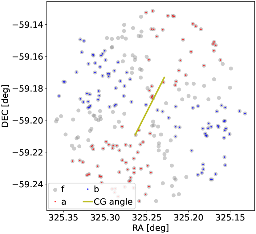
Figure 2: Example of making cuts for galaxies that are located around ($\pm 30\deg$) the directions of the major axis and the minor axis of the CG (DES Y1 redMaPPer cluster ID 503; $z=0.34$) in the selected Y3 shape catalogue for lensing analysis. For demonstration, we use a radial distance cut at $0.06\deg$ (1 Mpc). The red ($a$) and blue dots ($b$) show the major- and minor-axis samples respectively. The grey circles ($f$) show the source galaxies at all position angles. The yellow line is centred at the CG and shows the major axis direction of the CG. Different from Figure 1, here we use the CG’s 2D orientation to select the samples since the halo orientation is unknown. We apply the same position angle cut to the photometry catalogue.

3.5 Cluster stacking and division

We combine the signals from individual clusters to improve the statistics. Instead of combining the catalogues, we stack the cluster profiles to simplify the cluster selection (e.g. the binning of redshift and richness) and to reduce the computing resources; the two methods produces similar results.

When we stack the lensing profiles, we use the jackknife resampling method (Norberg et al., 2009; McClintock et al., 2019, and references therein) to estimate the error bar of the stacked (mean) result. Each profile is weighted by the reciprocal of the scatter.

We use kmeans_radec to divide the cluster sample into 100 similar regions, and each region roughly contains the same number of clusters. The kmeans_radec method runs the K-means algorithm on the unit sphere and addresses the cosmic variation and LSS.

In jackknife resampling, each time we skip one region and compute a stacked profile. We compute the covariance of those stacked profiles (the values in radial bins) and multiply the covariance by the number of regions minus 1 as the following:

$$\bar{s}(R_{i})=\frac{1}{K}\sum_{k=1}^{K}s_{\cancel{k}}(R_{i})~{};$$ (14)

$$C_{ij}=\frac{K-1}{K}\sum_{k=1}^{K}[s_{\cancel{k}}(R_{i})-\bar{s}(R_{i})][s_{\cancel{k}}(R_{j})-\bar{s}(R_{j})]~{}.$$ (15)

Here, $s$ is a stacked profile, $K$ is the number of regions while $\cancel{k}$ means removing the $k$th region. $i,j$ are the indices of radial bins, and $C_{ij}$ is the covariance term between the $i$th and $j$th radial bins.

We take the square root of each covariance matrix diagonal term as the stacked profile error bar at the corresponding radial bin, and we use the resampling mean ($\bar{s}$) as the stacked profile value, which is very close to the direct mean of all profiles. We use the same method to stack the number density and excess number density profiles without weight. The stacked profiles of all clusters are presented in Section 4.1.

We note that a few studies scale the radial distance by a cluster radius, e.g. the virial radius, before stacking. The advantage is that the clusters will be stacked at a ‘similar’ size and thus the result can have better statistics, but the disadvantage is that this hinders comparisons with studies that use physical lengths and different cluster detection techniques, and also introduces a measurement uncertainty. We will test this method in future work.

In addition, we divide the clusters along the richness (a mass proxy) or redshift direction with two bins to investigate the richness and redshift dependence of the results; the stacking is performed at each bin (Section 4.4).

For the richness division, we split the clusters into two bins so that the sum (of the richness) in the two richness bins are comparable. This results in more low clusters in the low richness bin, but produces more comparable SNRs in the measurements of both bins.

For redshift, however, we use the median value of cluster redshifts to split them into redshift bins. In theory, there will be more massive clusters (high richness) at low redshift because of merging, but massive clusters at high redshift are easier to be detected. Thus we expect similar richness distribution in the low and high redshift subsamples.

In Appendix B, we show an example of dividing the cluster sample into $2\times 2$ subsamples by both redshift and richness. The results have larger statistical noise, and thus in the main text we consider 2 bins on redshift or richness only.

Finally, we use a flow chart to outline our pipeline and summarize our method in Appendix C.

4 Results

In this section, we present our results as follows. First, we examine optical measurements of our galaxy cluster sample through stacked weak lensing and galaxy (excess) number density profiles. To extract signatures of triaxiality, we examine and compare axis-aligned profiles, defined as the stacked radial profiles in aximuthal slices along the CG major and minor axes, and we normalize them by a fiducial profile, which is a (randomly oriented) stacked profile that includes galaxies located at all position angles, to make the comparison more clear. We also relate these measurements to an ‘effective splashback’ radius, extracted from the fiducial profile. Then, we quantify any dependencies of triaxial signatures on the redshift or richness of galaxy clusters from our sample. Finally, we assess any differences in signature on the galaxy number density profiles that might depend on galaxy colour selection.

4.1 Weak lensing and galaxy density radial profiles

We first illustrate the stacked radial profiles of our main/canonical dataset, and differences in profile measurements due to triaxial shape. For most of our analysis, we use publicly available DES Y1 redMaPPer clusters (McClintock et al., 2019). Figure 3 shows the radial profiles of clusters subselected with $\max\{\texttt{P\_CEN}\}\geq 0.8$. This parameter indicates the confidence of the identified central galaxy (CG), which are more easily identified for more relaxed galaxy clusters. We therefore use P_CEN as a rough proxy for dynamical state; larger values of P_CEN also make it more likely that the orientation of the CG better aligns with that of the underlying dark matter halo. As described in Section 3.1, the entire sample has richness range across $20<\lambda<235$ and redshift range across $0.2<z<0.86$. For all panels in Figure 3, the black circles correspond to profile measurements using galaxies from the entire azimuthal range. The red squares and blue triangles respectively correspond to profile measurements in azimuthal slices (circular sectors) along the identified major and minor axes, which we refer to as ‘axis-aligned’ profiles. We use an angle cut of $\pm 30\deg$ on both sides for measurements in azimuthal slices. Note, we shift data points by 10% along the X-axis in each radial bin for visualization purposes.

The left column shows the (effective) excess surface density measurements, given by the lensing distortion in the tangential (top) and cross (bottom) directions with respect to the identified CGs as the galaxy cluster centres. We use the publicly released DES Y3 metacal shape catalogues for these measurements (Gatti et al., 2021). The tangential measurement shows a relatively clean monotonic decrease with cluster-centric radius. At $\sim 2$ Mpc, we see a subtle change in the profile slope of the tangential signal. This feature is analogous to the splashback feature observed in simulations (Diemer & Kravtsov, 2014; Xhakaj et al., 2020) and real data (Baxter et al., 2017; Chang et al., 2018). For measurements in the latter, authors fit models to the full density profile instead of simply extracting a position of steepening from the excess surface density as is done here.

These profiles also exhibit a systematic relative strength of signals at each radial bin, aside from the innermost bin, which has the largest noise for the azimuthal slices. The major axis ($a$) has the largest value, then the entire profile ($f$), then the minor axis ($b$). The cross signal is $\sim 10$ times smaller than the tangential and significantly noisier, showing no clear systematics, though exhibits a similar monotonically decreasing trend with radius; the relative strengths of the cross signal in each radial bin is much more difficult to disentangle due to the error bar size.

The right column shows number density profiles, measured from the DES DR2 photometry catalogue (Abbott et al., 2021). We use all galaxies that pass an initial selection based on SNR, flags for quality, and magnitude cuts to ensure completeness. In Section 4.5, we examine these profile trends by subselecting red-sequence galaxies. The top right profiles correspond to the projected number density of galaxies $n(R)$. Here, the error bars are small enough at all radial bins to see the systematic relative strength of signals even in the left-most radial bin. Again, the measurement limited to the azimuthal slice along the major axis is the largest, then the measurement for the entire azimuthal range is in the middle, while the measurement for the slice along the minor axis is the smallest. We see a precipitous drop in number density until $\sim 1$ Mpc, which encompasses cluster member galaxies. The bottom right profiles correspond to the excess number density of galaxies, which we define as $\Delta n(R)=\overline{n}(<R)-n(R)$. The excess number density is a closer analog to the lensing signal, as it reduces the contribution from foreground and background galaxies. Here, we see a more continuous decline until $\sim 10$ Mpc, and a subtle change in slope around $\sim 2$ Mpc that plausibly corresponds to the same splashback feature in the tangential excess surface mass density profile. The systematic relationship between the different azimuthal slices is consistent within radial bins inside the $\sim 10$ Mpc range. Outside of this, we expect stacked large scale structure traced by galaxies to have more azimuthal symmetry.

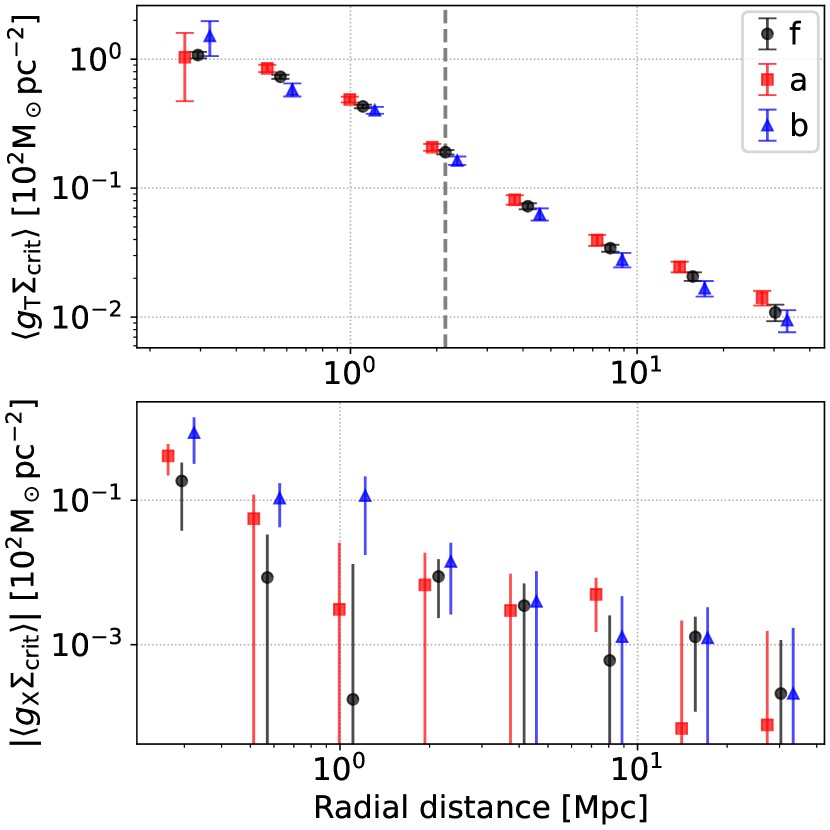
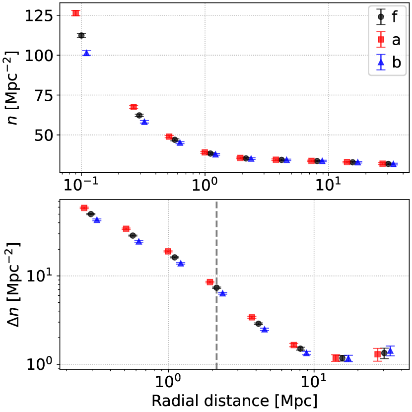
Figure 3: Stacked profiles from our main/canonical dataset of DES Y1 redMaPPer clusters ($\max\{\texttt{P\_CEN}\}\geq 0.8$ for each) across all available redshifts ($0.2<z<0.86$) and richness ($20<\lambda<235$): tangential excess surface mass density (top left), cross excess surface mass density (bottom left), galaxy number density (top right), differential/excess galaxy number density (bottom right). Here $f$ is the fiducial profile measurement using galaxies from the entire azimuthal range (4289 clusters; 11 out of 4300 are not in this footprint), while $a$ and $b$ show the samples around the directions of the major and minor axes of the central galaxy of individual clusters (4217 clusters; 72 out of 4289 failed to match the shape catalogue to obtain the central galaxy angle due to ambiguity e.g. blending). In all cases with sufficient signal-to-noise ratios for small enough error bars, measurements along the major axes exceed that of those made for the entire azimuthal range, and measurements along the minor axes are less than that made for the entire azimuthal range. The vertical dashed line in each figure gives the local minimum of the logarithmic derivative of the fiducial profile of the cluster sample. For visualization, we add caps to the error bars in some graphs, and we shift the $a$ and $b$ points horizontally by 10% but fix the $f$ points; the X-coordinates are bin centres (same below).

4.2 Axis-aligned profile trends

We now discuss relative features in axis-aligned profiles, measured in azimuthal slices aligned with the major and minor axes. The slices span $\pm 30$ degrees, centred on the CG major ($a$) or minor axis ($b$). Figure 4 illustrates the profiles measured along the major axis (red squares) and along the minor axis (blue triangles), each normalized with respect to the fiducial profile ($f$) measured for the entire azimuthal range (the measurement made with galaxies that are at all position angles), with error bars estimated by uncertainty propagation.

The left panel of Figure 4 shows the normalized excess surface density profiles. These profiles probe the projected mass distribution. Aside from the innermost radial bin, which has very large error bars due to the low lensing SNR produced by limited source galaxies, the major axis measurements, $a$, are larger than all measurements made for the entire azimuthal range, $f$. Data points of $a/f$, including errors, all sit above a ratio of 1. The reverse is true for the measurements along the minor axis. All $b/f$ ratios including the error bars (except for the measurement in the innermost radial bin), mostly sit below a ratio of 1. The offsets from 1 in $a/f$ and $b/f$ are both $\sim 10-20\%$.

Interestingly, we see hints of a ‘necking’ feature; the profiles exhibit a radial trend where $a/f$ and $b/f$ data points converge towards 1 at a radial distance of about $\sim 1-2$ Mpc, before separating again. We see hints of this effect with other datasets and also in subsamples of galaxy clusters in narrower richness and redshift bins (see Section 4.4). The location of this ‘neck’ is consistent with simulation measurements of surface mass density/lensing signal of triaxial haloes made by Osato et al. (2018) and Zhang et al. (2023), who also found a ‘neck’ feature around the transition between the one-halo and two-halo dominated regimes. However, their methods to extract triaxial signatures are different from ours – they considered source galaxies at all position angles when fixing the angle between the halo major axis and the line of sight, while we consider signals along the CG (projected) major- and minor-axis directions only. Our measurements may be the first observational evidence of this ‘necking’ feature existing in the triaxial mass distribution around clusters. In the left panel of Figure 4, the similarity in both axes-aligned measurements at $\sim 1$ Mpc is likely due to this location corresponding to an effective edge of the clusters associated with the approximate average splashback locations. Outside of $\sim 1$ Mpc, cluster-feeding filaments govern the mass distribution. Filaments likely align with the orientation of the triaxial cluster (and the CG), leading to another boost in the separation between the two axes-aligned profiles (Tempel et al., 2015; Gouin et al., 2020).

The right panel of Figure 4 shows the normalized excess galaxy number density profiles. While luminous galaxies trace underlying mass distributions, they are biased tracers and we do not expect a perfect correspondence (Kauffmann et al., 1997; Coil, 2013). The error bars of these normalized profiles are much smaller than those in the normalized tangential excess surface density profiles. Here, we see an almost flat offset until about $\sim 8$ Mpc. Inside this radius, the profile measured along the major axis is $\sim 20\%$ larger than that of the profile measured using all galaxies and the profile measured along the minor-axis is $\sim 15\%$ smaller than that of the profile measured using all galaxies.

Compared with the normalized axis-aligned profiles of the tangential excess surface density, the values normalized in the excess galaxy density measurements are similar. But, the ‘necking’ feature in the normalized axis-aligned excess galaxy density profiles occurs at a much larger radius of $\sim 10-20$ Mpc, well outside the environments of each galaxy cluster. Ratios at larger radii converge to unity quickly. Overall, the ‘necking’ feature corresponds to the average radial location where axis-aligned profile measurements appear to become more similar to one another. The ‘neck’ location occurs near the effective splashback location for the tangential excess surface density measurements (between $\sim 1-5$ Mpc when we vary the richness), while the feature for the excess number density measurements does not appear to have the same association. We see hints that the ratio offset slightly decreases near the effective splashback radius derived from the fiducial excess number density profile. We further discuss these in Section 4.4, where we examine how redshift and richness impact these features.

We note that these observational trends reasonably correspond to those described in the toy model of an elliptical NFW profile with axis ratio 2/3, laid out in Section 2, although an elliptical two-halo term may be necessary for explaining the ‘necking’ feature. The result illustrated in Figure 1 also shows a relatively flat offset in ratio values by $\sim 15\%$ around 1 in tangential reduced shear and excess convergence.

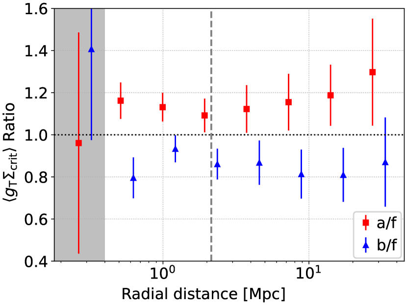
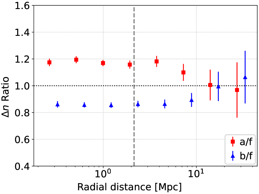
Figure 4: Normalized axis-aligned tangential excess surface density (left) and the excess galaxy number density (right) profiles for the canonical dataset (same data as shown in Figure 3). We measure these along the major (red squares) and minor (blue triangles) axes of the central galaxy of each galaxy cluster and normalize to the measurement made across the entire azimuthal range (fiducial). These correspond to ratios between the (stacked) profiles presented in Figure 3. In each panel the grey vertical dashed line shows the location of the local minimum of the logarithmic derivative of the respective fiducial profile (effective splashback radius).

4.3 ‘Effective splashback’: Transition locations in projected profiles

Here, we illustrate features in the stacked profiles that correspond to a transition in the logarithmic derivative of each profile of the optical signature. We call this an ‘effective splashback’ (in 2D), as this is a similar method used by More et al. (2016); Chang et al. (2018); Sunayama & More (2019). However, previous works have identified the splashback radius from deprojected profiles to model the 3-dimensional mass or galaxy density distribution. We illustrated the transition location in the projected surface mass density profiles and the excess/differential galaxy number density profile, respectively as vertical dashed lines. Note, the location of the ‘effective splashback’ location occurs in the same radial bin for both measured profiles. Given the coarseness in radial binning, this is consistent with the results from Chang et al. (2018), who found agreement between the 3D splashback locations derived from galaxy density and lensing data respectively; note they used comoving coordinates to improve the detection of the 3D splashback feature, but we use physical distances since the goal of this paper is to study cluster triaxiality.

In Figure 4, we can compare the effective splashback locations with trends in the normalized axis-aligned profiles – $a/f$ and $b/f$ ratios. In the left panel, the ratio values for the excess surface density exhibit a ‘necking’ feature near the effective splashback radius, at a radius of $\sim 1-2$ Mpc. In the right panel, a similar feature for the profile ratios of $\Delta n$ occurs at around $\sim 10-20$ Mpc. We can attribute the difference in ‘neck’ location in the ratios for each of the two profiles to the fact that galaxies associated with the cluster will trace the structure on larger scales. The distribution of the associated galaxies likely sit in filaments feeding into the cluster, tracing the direction of the major axis to even larger radial distances. On the other hand, both the lensing ‘necking’ feature and the effective splashback locations more closely indicate the edges of the cluster mass distribution.

To identify the ‘effective splashback’ in each profile, we calculate the derivative over 12 radial bins illustrated in Figure 5. Note, we calculate the effective splashback with 12 instead of the 8 radial bins shown in the figures from Section 4.1. While the increase in the number of radial bins (by 50%) worsens the noise, particularly for the excess surface mass density profiles, this allows us to identify a more accurate location of a ‘dip’ in the profile derivative ($\sim 2$ Mpc). There are signs that the local minimum of the minor-axis sample ($\sim 2$ Mpc) is smaller than the one of the major-axis sample ($\sim 4$ Mpc) both in the lensing and excess number density ratios (as indicated by the arrows in Figure 5), which physically makes sense since a cluster is expected to be ‘longer’ along its major axis; but these phenomena could be caused by noise as well.

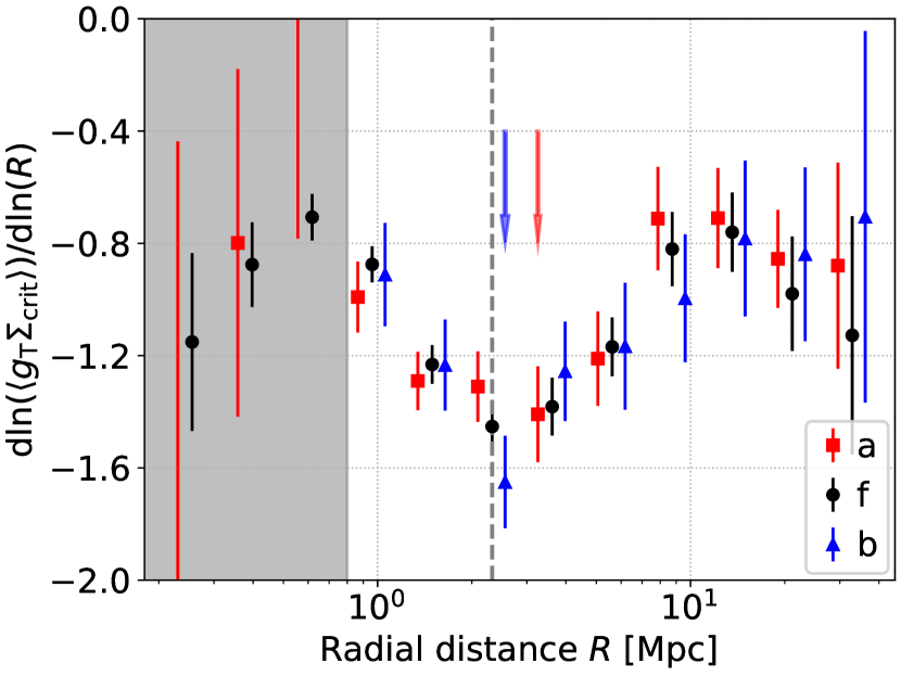
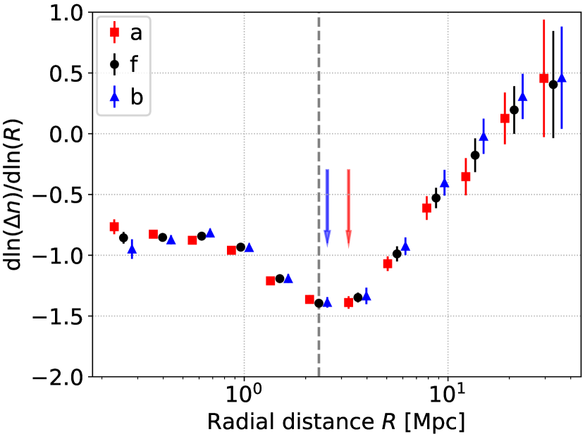
Figure 5: Left: Logarithmic derivative profile of the effective excess surface density. Because $\langle g_{\textrm{T}}\Sigma_{\textrm{crit}}\rangle$ of the minor-axis sample ($b$) is negative at the second radial bin, we omit the values at that bin and neighbouring bins. Right: Logarithmic derivative profile of the excess number density. The vertical dashed line in each panel indicates the local minimum for the fiducial sample between 1 and 10 Mpc, corresponding to an ‘effective splashback’ location. The red and blue arrows indicate the local minimums for the major-axis sample and the minor-axis sample respectively.

4.4 Triaxial signature dependency on redshift and richness

In this subsection, we examine how the normalized axis-aligned profiles discussed in Section 4.2 behave in different richness and redshift ranges. Figure 6 shows normalized profiles of the lensing distortion, defined by the tangential excess surface density. We subdivide our cluster sample from Figure 3 into only two subsamples in order to preserve sufficient SNR for a measurable difference between the major- and minor-axis measurements, respectively red squares, indicated as $a/f$ and blue triangles, indicated as $b/f$.

The top row illustrates the difference between a lower redshift subsample (top left: $0.2<z<0.47$) and a higher redshift subsample (top right: $0.47<z<0.86$). The radial location of the ‘neck’ in the low redshift subsample is consistent with that of the entire sample, shown in Figure 4 at $R_{\mathrm{neck}}\sim 1-2$ Mpc. This is not surprising, given that the low redshift subsample likely drives most of the signal in the total stack. The high redshift subsample unfortunately has too large error bars to clearly show the location of the ‘neck’, but may be anywhere between the third and fifth radial bin (excluding the shaded bin; $R_{\mathrm{neck}}\sim 2-8$ Mpc).

In contrast, there is a clearer difference in the location of the ‘neck’ between low and high richness objects. The bottom row illustrates the difference between the lower richness subsample (bottom left: $20<\lambda<33$) and the higher richness subsample (bottom right: $33<\lambda<235$). The neck in the low richness subsample is consistent with that of the entire sample at $R_{\mathrm{neck}}\sim 1-2$ Mpc. However, the feature in the high richness subsample occurs closer to $R_{\mathrm{neck}}\sim 4-5$ Mpc. We have also included the corresponding ‘effective splashback’ locations derived by respective fiducial profiles for each subsample shown in the panels. We note that the effective splashback location for the high richness subsample is also at a larger radius ($\sim 4$ Mpc), similar to the ‘neck’. The larger radial locations of both the neck and the effective splashback feature are consistent with the fact that the larger richness subsample has more massive clusters with larger characteristic radii.

One additional reason for the location of the ‘necking’ feature in the excess surface mass density ratios and the correspondence to the effective splashback location may be that the excess surface mass density is sensitive to projection effects from nearby correlated LSS along the line-of-sight. These structures would be influenced by the galaxy cluster environment and therefore correlated with the galaxy cluster location. But, these structures may not correspond to the primary filaments aligned with the cluster axes, and their orientations are more randomly distributed. The random orientations introduce a rounding effect on the weak lensing profile ratios that produces the ‘necking’ feature washing out the triaxial signature, but not the galaxy distribution. Beyond the radial location of the ‘neck’, this LSS contribution to the mass along the line of sight becomes less significant, leading to an overall projected mass that aligns with the central halo; thus, the triaxial signature in the lensing signal recovers at larger radii. This ‘necking’/rounding feature in the normalized lensing profiles cannot be produced by the cluster halo and primary filaments only, because otherwise the normalized galaxy density should show a clear ‘neck’ at the same location. It is not generated by uncorrelated LSS either, which is randomly distributed and would wash out the lensing triaxial signature quickly.

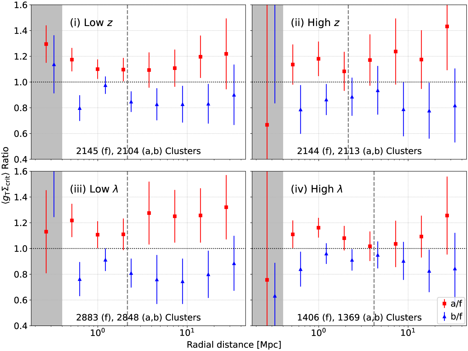
Figure 6: Normalized axis-aligned profiles showing the ratios of the excess surface mass density for subsamples of our canonical dataset. Major axis profiles are in red squares, and minor axes profiles are in blue triangles. We plot both results for the tangential lensing distortion and the excess number density (next figure) for comparison. The top left (i)/right (ii) panels show the difference between low/high redshifts, while the bottom left (iii)/right (iv) panels give the difference between low/high richness. The ‘necking’ feature of both left-hand panels (low redshift and low richness) occur at smaller radii compared with the locations of that feature in the right-hand panels. Annotations indicate the number of clusters used in the redshift or richness bin for the ‘effective splashback (dashed line)’ measurement ($f$; fiducial), or for the ratio profile measurement ($a,b$; major, minor axes). Not all clusters have a clear CG to use for axis identification due to blending and/or the presence of multiple CGs.

Figure 7 shows normalized profiles of the excess number density, measured in azimuthal slices along the major (red squares, indicated as $a/f$) and minor (blue triangles, indicated as $b/f$) axes. Again, we normalize profiles with respect to the measurement made with all galaxies ($f$) in that radial bin. The excess number density profiles have much smaller error bars compared with the excess surface density profiles. The top and bottom rows correspond to the same respective redshift and richness subsamples as in Figure 6. In Appendix B we consider a further division that splits clusters by both redshift and richness but the results are noisier. Here we also present the ‘effecitve splashback’ location of the fiducial excess number density profile in each cluster subsample, which is still consistent with the lensing results.

While the ‘neck’ locations in the tangential excess surface density measurements occur near the effective splashback location in each subsample, the similar ‘necking’ feature occurs at much larger radii for the analogous measurement in excess number density. The ‘necking’ feature of the low redshift subsample occurs between the antepenultimate and the penultimate radial bins, $R_{\mathrm{neck}}\sim 10$ Mpc. The low richness subsample has hints of $R_{\mathrm{neck}}\sim 10$ Mpc as well. The locations of the ‘neck’ in other subsamples are more closer to the corresponding location for the entire sample: they sit closer to the penultimate bin, with $R_{\mathrm{neck}}\sim 10-20$ Mpc.

These trends indicate that the excess number density measurements along each axis do not converge to one another until well outside the cluster region, at a radial distance of $\gtrsim 10~{}$Mpc, regardless of effective splashback location. In other words, our selection of cluster galaxies more strongly traces signatures of triaxiality to larger radii. This is likely due to the fact that our galaxy selection for the excess number density profiles is comprised of galaxies associated with the galaxy cluster, both cluster members and accreting galaxies at the same redshift. These galaxies would trace the cluster-feeding filaments that drive the underlying shape of the cluster.

Note, the potential rounding effect from LSS that could contribute to the ‘necking’ feature in the excess surface mass density ratio profiles would not affect the galaxy density. Correlated structures not associated with the primary filaments feeding the galaxy cluster would be less likely to contain galaxies (at least bright ones) because of their low masses. Thus, the ‘necking’ feature in the galaxy distribution is solely determined by the primary filamentary structures (which are more massive) at even larger radii.

Also, signatures of triaxiality seem to completely disappear after the ‘necking’ feature in the galaxy distribution, whereas there is still a systematic offset in ratios at large radii for the excess surface mass density profiles. For the radial distances $\gtrsim 10$ Mpc, galaxies that trace the DM filaments are likely lower mass objects below our detection threshold. Thus, the triaxial signature of structure surrounding galaxy clusters disappears at the largest radii in the excess galaxy distribution but not in the excess surface mass distribution. In the future, we will re-examine these in cosmological simulations.

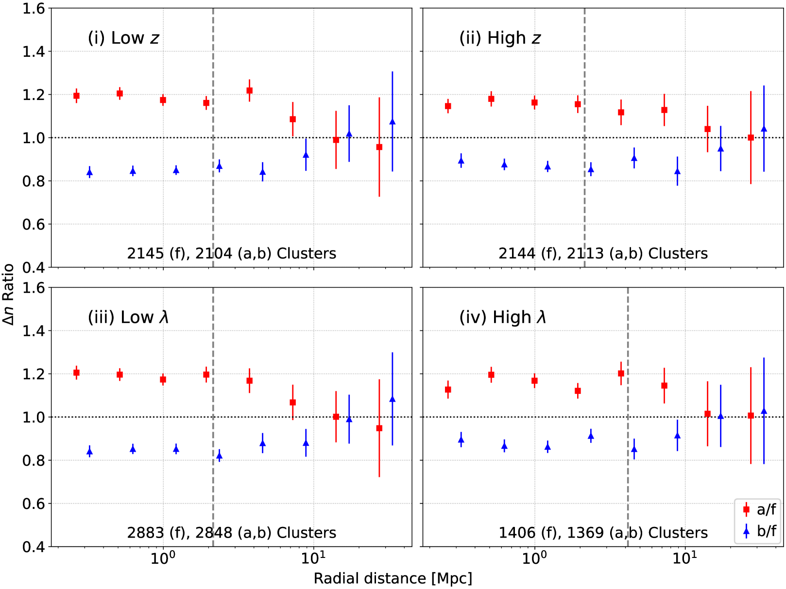
Figure 7: Normalized axis-aligned profiles showing the ratios of the excess number density for subsamples of our canonical dataset. Each panel shows the measurement for the same subsamples as in Figure 6: the top left (i)/right (ii) panels show the difference between low/high redshifts, while the bottom left (iii)/right (iv) panels give the difference between low/high richness. Again, low redshift or small richness subsamples exhibit smaller radii of convergence/‘neck’.

Despite the wide subselection in redshift and richness, we can summarize some (non)-trends for the lensing and excess number density results. First, the ‘effective splashback’ location does not have a clear dependence on redshift. Both subsamples divided by redshift have similar distributions in richness, and therefore similar distributions in mass (Melchior et al., 2017; McClintock et al., 2019). Any trends would therefore be due to redshift dependence in non-mass dependent features of the subsamples, such as dynamical state. While we expect higher redshift objects to be more dynamically unrelaxed, we do not see any measurable difference of ‘effective splashback’ locations within the radial bins and redshift subsamples measured. We do find that the ‘neck’ location seems to show up in a larger radius in the higher redshift subsample. Second, both the ‘effective splashback’ location and the ‘neck’ location occur at noticeably larger radii for the high richness subsample, consistent with the fact that high richness clusters are more massive with larger sizes and splashback radii. The corresponding increase in the ‘neck’ radii of the lensing signal is consistent with the assertion that the ‘neck’ occurs near the average edge of the cluster mass distribution, where the tangential excess surface density along the major axis is more similar to that along the minor axis. For galaxy number density, this means a larger cluster tends to have longer filamentary structure connected to it. Third, we do not see the same association of the physical scale between the ‘effective splashback’ and ‘neck’ location for the excess surface number density of galaxies as the excess surface mass density, likely due to the fact that our galaxy selection more closely traces the primary filaments and associated triaxial alignment near the cluster edge, while the lensing signal is more affected by the projection effect. Finally, the ratio values (as a proxy of the mean halo triaxiality) do not strongly depend on redshift and richness. The high richness clusters seem to have ratios closer to 1 in the lensing results (i.e. rounder shapes) but the ‘necking’ feature also affects the ratio, and the excess number density ratio does not show a similar change. Still the ratios along the two axes are nearly symmetric with respect to unity; this asymmetry is mainly due to the fact that the azimuthally averaged signal ($f$) includes regions in addition to the ones along the major ($a$) and minor ($b$) axes (Figure 2).

4.5 Red-sequence galaxies distribution

In this subsection, we examine how galaxy populations impact the signature of triaxiality on the axis-aligned excess number density profile measurements. We split galaxies associated with each cluster into a red-sequence and non-red-sequence population, identified by the redMaPPer colours and magnitude limits: for each cluster, we compute the median and the scatter of colour $r-i$ and $i-z$, and the magnitude limit in $r,i,z$ of the cluster member galaxies reported by redMaPPer ($g-r$ has a larger scatter), and then select the galaxies in the DES DR2 catalogue (pre-selected by the method in Section 3.3) using those magnitude limits and 1.5 times the standard deviation around the median of each colour. The reason for selecting galaxies in the DES DR2 catalogue rather than directly using the redMaPPer cluster member catalogue is that the member galaxies in the redMaPPer catalogue have a radial distance limit $R_{\lambda}\sim 1$ Mpc, which is close to the virial radius (McClintock et al., 2019, and references therein). Note, galaxies beyond the virial radius of each galaxy cluster are no longer cluster member galaxies, but are otherwise associated with the nearby filaments, and are likely to accrete.

Figure 8 shows the excess number density ratios of the signal along the major (red squares) and minor (blue triangles) axes to the fiducial signal (generated by galaxies in all directions) as functions of distance from cluster centres. The left panel shows this ratio for excess number density profiles measured with red-sequence galaxies associated with the galaxy clusters, and the right panel for profiles measured with all other associated galaxies. The primary difference between the two is in the ‘neck’ location. For red-sequence galaxies, the necking feature occurs in the largest radial bin, $\sim 30$ Mpc. The necking feature in profile ratios from all other associated galaxies occurs closer to $\sim 10$ Mpc. These results are consistent with measurements from Zhang et al. (2013), who found that red galaxies better trace large scale structure and intercluster filaments. Specifically, luminous red galaxies (LRGs; or red-sequence galaxies in clusters) are commonly used tracers for LSS and the matter distribution in our universe. In cluster environments, the distribution of these objects trace triaxial signatures to larger radii than other galaxies. Figure 8 illustrates that red-sequence galaxies in our sample do in fact trace the extended mass distribution of triaxial galaxy clusters to larger radii.

We note that the effective splashback location appears in the same radial bin for both profiles (and the same bin for the whole sample, Figure 4), shown with the vertical dashed line. Interestingly, the shift in ‘neck’ location does not track any shifts in the effective splashback location, contrary to the relationship between the two features in Figures 6 and 7 for high richness clusters. The stability of the effective splashback radius is consistent with conclusion from Baxter et al. (2017), who showed that the location in profile steepening is consistent between the red and blue galaxies in their galaxy cluster sample considered. The effective splashback location of galaxies off the red sequence could come from a population of ‘green’ galaxies that are quenching star formation as they enter the cluster and start to rotate around the cluster centre (Shin et al., 2019).

Additionally, we find the ratio values do not have a strong dependence on galaxy colours and are generally flat at small radii. The galaxies off the red sequence show a smaller offset from unity but with larger error bars. Again, the ratios along the two axes are nearly symmetric with respect to 1.

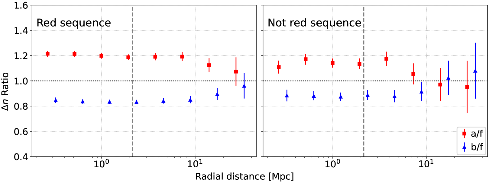
Figure 8: Normalized axis-aligned profiles showing ratios of excess number density for red-sequence (left) and non-red-sequence (right) galaxies. Note, the location of the ‘effective splashback’ radial bin (the grey vertical dashed line) does not measurably change with the galaxy sample selection, but red-sequence galaxies retain triaxial signatures in these profiles to larger radii.

5 Discussion

5.1 Robustness of results

Here we test the robustness of our results by adjusting the sources of catalogues (generated by different measurement methods) one by one. The same physical quantity should have similar results no matter what measurement methods are used.

5.1.1 Robustness to lensing signature and number density measurements: Legacy Surveys shapes and photometry

We use the Legacy Surveys DR9 shape and photo-z measurements for building lensing profiles and Legacy Surveys DR9 photometry for building excess number density profiles, but still use the DES Y1 redMaPPer cluster catalogue. The CG angles still come from the DES Y3 shapes. In Figure 9, we show the normalized axis-aligned profiles, with the dashed vertical line showing the local minimum of the logarithmic derivative of each LS fiducial profile (both effective splashback locations are at $\sim 2$ Mpc). The results are consistent with the ones derived from the DES Y3 shapes and DR2 photometry: a clear (and nearly symmetric) difference between the major- and minor-axis samples, with ratio values spanning $\sim 10-20\%$ around 1; a probable ‘necking’ feature at $\sim 1-2$ Mpc in the excess surface mass density ratio (though the error bar of the minor-axis sample is large at the second radial bin); an excess number density ratio ‘neck’ at $\sim 10-20$ Mpc.

We also test and find that using DES Y1 shape catalogue (Zuntz et al., 2018), photo-z catalogue (Hoyle et al., 2018), and DES DR1 photometry (Abbott et al., 2018) produces consistent but noisier results, and the reason is that DES Y3 shape catalog has improved measurement methods and DES DR2 photometry catalog has improved depth.

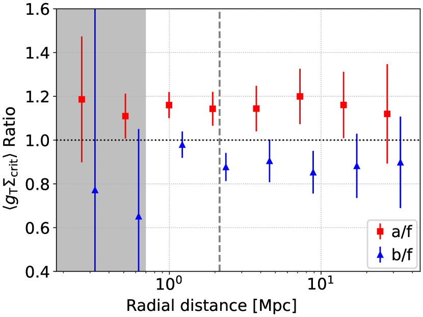
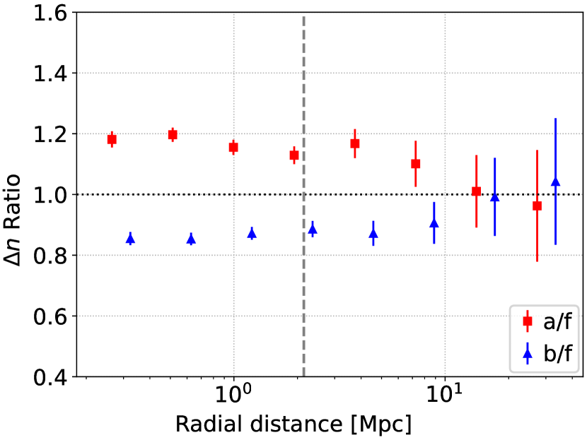
Figure 9: Normalized axis-aligned profiles showing excess surface mass density ratios (left) and excess galaxy number density ratios (right) using the Legacy Surveys DR9 catalogues but DES Y1 redMaPPer cluster catalogue. The fiducial ($f$) profile measurement uses galaxies at all position angles (4300 clusters); the major- ($a$) or minor-axis ($b$) profile measurement uses 4217 clusters. The cluster sample is selected by $\max\{\texttt{P\_CEN}\}\geq 0.8$ and spans richness $20<\lambda<235$ and redshift $0.2<z<0.86$.

5.1.2 Robustness across CG angle measurements methods

We compare the measurements of the CG angle using the DES Y3 and LS DR9 catalogues. We find the two methods produce consistent results (Figure 10).

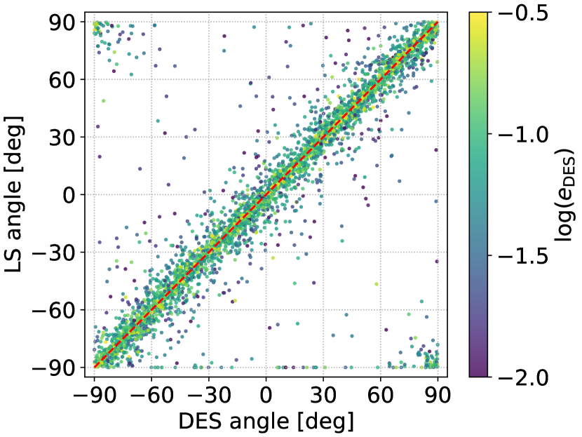
Figure 10: Comparison between the CG angles derived from the DES Y3 metacalibration shapes (X-axis) and the Legacy Surveys (LS) DR9 Tractor model fit shapes (Y-axis), colour-coded by the logarithm to the base 10 of the DES ellipticity, to illustrate the robustness of the CG angle measurements for the selected DES Y1 redMaPPer clusters. Large scatters happen at small ellipticity (caused by float errors) or near angle $\pm 90\deg$ (which are equivalent). Some CGs have the model type REX and thus 0 ellipticity and -90 $\deg$ angle in LS; they are partially caused by blending. Only 0.7% of the DES CGs do not have the counterpart in LS. The red dashed diagonal line is for reference.

We also check the CG angle distributions in redshift and richness subsamples (Figure 11). The distributions are generally uniform as expected – we find no preferential 2D orientation of the CGs, and thus no selection bias when we make cuts on the catalogues based on the CG angle. Since the CG angles derived from DES and LS are consistent, we only use the DES angles in this work.

Additionally, we test and find that the difference between the CG angles of any two clusters and their angular separation does not correlate in our cluster sample; the distribution of the CG angle difference is also uniform.

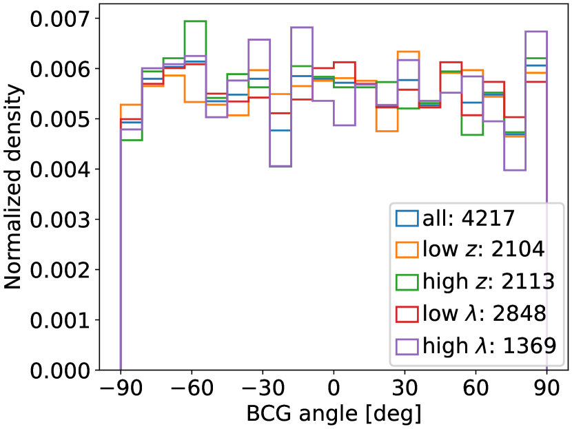
Figure 11: Histogram of the CG angles in different redshift/richness subsamples (with the number of clusters in each set). The histograms are normalized to show the uniformity.

5.2 Projection of CGs and clusters

The CG angle we measure is a projection of its 3D orientation. Though the offset between the orientation and the projection plane is likely averaged out after stacking, the detected halo ellipticity can be lowered due to the projection. Moreover, an offset between the CG angle and the halo orientation exists (Shin et al., 2018).

So far we have assumed the projected isodensity contours are concentric and aligned. Commonly, the contour ellipticity is assumed to be constant as well (homoeoidal), and any projection of a homoeoidal model is still homoeoidal; the projection of a varying ellipticity model produces ‘twisted’ contours (e.g. Schramm, 1990, and references therein). Since we stack the clusters, the twisting is likely averaged out, but the ellipticity can still vary with the radial distance (and gradually decreases to zero at sufficiently large radii).

In this paper we test two directions – the major- and minor-axis directions of CG. Other angles, e.g. $45\deg$, from the major and minor axes can also be studied to check the symmetry, but this is beyond the scope of this paper – we leave it to future work.

5.3 Correlation between lensing signature and number density: Mass-number ratio

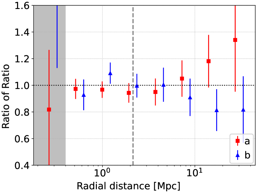
Figure 12: Ratio between the normalized axis-aligned profiles of effective excess surface mass density and the excess number density. The legend shows the two samples along the major axis ($a$) and minor axis ($b$) respectively. The two ratios are nearly unity at small radii. At large radii, they diverge because the lensing signal continues to exhibit difference between the major and minor axes, and the number densities appear to be more circularized.

One interesting perspective from our results is the confirmation of the simultaneous influence of cluster triaxiality on both the cluster galaxy distribution and cluster weak lensing signal, even at a very large radius ($\sim 10-20$ Mpc); on average when a cluster’s weak lensing signal is measured to be higher in one direction, its galaxy density is also higher in that direction. Similarly, a few previous studies have studied the correlation between the lensing signals and galaxy overdensities using simulations, and they find this type of correlation creates a selection effect – clusters identified in an optical catalogue using a galaxy density criterion is likely to have a biased lensing signal. But we need to point out that, in previous studies, the lensing signals and galaxy overdensities are usually measured by the average over all position angles on the plane of sky (PoS), while we study them along the cluster’s projected major and minor axes (traced by CG) on PoS only. For example, Zhang et al. (2023) studied the correlation between the clusters’ richness (a probabilistic red-sequence galaxy count) and their projected radial mass densities of triaxial dark matter haloes in simulations. They concluded that triaxial haloes, when their major axis is aligned with line of sight, have both a higher richness estimation – which is a galaxy overdensity measurement – and a boosted lensing signal than expected from their masses. Our analysis provides additional observational evidence to their finding; we find that along the major (or minor) axis of a galaxy cluster, both the cluster’s galaxy overdensities and mass overdensities – as measured by weak lensing – will appear to be higher (or lower), and this simultaneous increase (or decrease) extends to at least $\sim 10-20$ Mpc on average.

More interestingly, we show how the cluster’s weak lensing signals are correlated with the galaxy overdensity measurements, depending on the radius range. In previous sections, while the cluster’s lensing signals are higher along the major axis throughout the whole 0.4 to 40 Mpc radial range by $\sim 20\%$, the elevation in the galaxy overdensity along the same axis does not stay elevated as far. Furthermore, along the major axis, the red-sequence galaxy overdensity is elevated by $\sim 20\%$ only to $\sim 20$ Mpc, while the overdensity of non-red-sequence galaxies stays elevated at the same level only to $\lesssim 10$ Mpc. This radial-dependent change in the lensing signals and galaxy overdensities indicates that variations in the two observables are more correlated at small scales, but they may become uncorrelated at large scales.

This can be further illustrated in Figure 12, which compares the lensing/effective excess surface density ($\widetilde{\Delta\Sigma}$) versus photometry/excess number density ($\Delta n$), and shows the ratio of the previous two ratios, i.e., $[a/f]_{\widetilde{\Delta\Sigma}}/[a/f]_{\Delta n}$ or $[b/f]_{\widetilde{\Delta\Sigma}}/[b/f]_{\Delta n}$ (derived from the two plots in Figure 4). This new ratio is nearly unity at small radii, indicating an almost perfectly-correlated increase/decrease in both lensing signals and galaxy overdensities along each axis, but the ratio gradually diverges after the effective splashback radius (especially after $\sim 10$ Mpc), indicating a weakening in the correlation. There are also hints that this ratio is even smaller (for the $a$ sample) or larger (for the $b$ sample) than 1 near the cluster centre, indicating a different degree of correlation towards the cluster core.

In galaxy cluster observations, the correlations between lensing signals and galaxy overdensities can be worsened by projections along the line of sight (LoS). When a triaxial halo is observed, if we consider the azimuthal average over all position angles on PoS, its lensing signals may appear to be stronger or weaker depending on whether its major or minor axis is aligned along LoS, and so is its observed galaxy overdensity. In our analysis, we study the signals along the clusters’ major and minor axes on PoS, which is perpendicular to LoS, using the CG angle. If the same clusters are rotated to have their major axes nearly aligned with LoS, we would still expect their lensing signals to remain higher than the average of the results of all rotation angles (or the result of a spherically-symmetrical galaxy cluster with the same mass), although now this is caused by the column/surface density being higher (under the thin lens approximation) and thus not necessarily still by $\sim 20\%$. Also, we expect that this boost is caused by the projection of not only the cluster triaxial halo but also the nearby aligned LSS. This boost can extend to large radii on PoS when the major axis is slightly tilted from LoS, since we find the connection between the triaxial halo and nearby filaments can extend to $\sim 40$ Mpc. The case will be similar for galaxy overdensities, but we expect the boost will extend to smaller radii, because the alignment between the triaxial cluster galaxy distribution and nearby LSS extend to only $\sim 10-20$ Mpc in our results. Similar arguments can be made if the same clusters in our analysis are rotated to have their minor axes aligned with LoS. In other words, when considering projection along LoS, the clusters’ observed lensing signals and galaxy overdensities may not be 1:1 correlated, and the lensing signals are likely to be more biased than the galaxy overdensities at very large radii.

Moving forward, in recent years, the correlation between lensing signals and galaxy overdensities and its induced selection effect has become a crucial element of cluster cosmology analysis, and the selection effect has been extensively studied in simulations. However, our analysis is the first to provide insights into this correlation effect using observational data towards $\gtrsim 20$ Mpc. As simulation studies of the correlations are often limited by their accuracy to match observational data, our method can provide crucial checks in the simulation-based conclusions. Further, such a correlation may exist between a variety of cluster observations, including X-ray/SZ versus lensing/richness, etc. Our analysis provides a new perspective to put observation-based constraints on this correlation effect. Moreover, our method may also help to provide insights into LSS galaxy bias.

6 Summary and Prospects

In this work, we have studied galaxy cluster triaxiality by using a sub-sample of DES Y1 redMaPPer clusters that have well-defined CGs. We use the CG major and minor axes as proxies for the underlying galaxy cluster triaxial mass distribution. We use these axes to build axis-aligned (stacked) profiles of (effective) excess surface mass density ($\widetilde{\Delta\Sigma}$) via lensing, and excess galaxy number density ($\Delta n$) via photometry. We found the following in our measurements:

• There is a clear difference between each axis-aligned profile in both lensing signatures and galaxy distributions, especially after normalizing the profiles by the azimuthally-averaged stacked profile (as the fiducial) that considers the galaxies at all position angles.

• The normalized profiles along the two directions are nearly symmetric with respect to unity – an increase along the major-axis direction for both lensing signatures and galaxy distributions, and an decrease along the minor-axis direction.

• The mean difference between each axis-aligned profile and the fiducial profile is $\sim\pm 10-20\%$ for both lensing signals and galaxy overdensities, starting from the inner region of the clusters ($\sim 0.4$ Mpc) to nearby groups/clusters and filaments/LSS ($\sim 10-20$ Mpc).

• The difference between the axis-aligned profiles and the fiducial profiles extends further out in dark matter than galaxies (the ratio of their physical lengths is $\sim 2$).

• Since the CG orientation approximately traces the cluster’s halo orientation, our results shows that nearly relaxed clusters still have clear signs of triaxiality in the axis-aligned profiles, which is consistent with previous studies.

• We did not see a strong dependence of the axis-aligned profile behavior on the cluster mass or on the cluster redshift in the two richness/redshifts bins we examined. However, the effective splashback radius ($\sim 2-4$ Mpc) – the location of a local minimum of the fiducial profile’s derivative in the logarithmic space, does increase as the richness increases (i.e. a more massive cluster), as expected.

• The normalized mean lensing profile shows a decrease in the triaxiality signature near the effective splashback location but it increases again afterwards (a ‘necking’ feature); while the triaxiality signature shown in the normalized mean excess galaxy number density is nearly constant and disappears soon after $\sim 10$ Mpc.

• We also noted that the red-sequence galaxy distribution showed the same triaxiality feature but extended further out than the others, and therefore the volume they span is between that of DM and regular galaxies; the reason is likely that these red galaxies trace the matter distribution better.

The primary datasets for our analysis are the DES Y3 and DR2 catalogues. To test the robustness of our results, we also used another dataset for studying the lensing signal and the galaxy number density – the LS DR9 catalogues, and found consistency between the results of DES and LS, though they use different shape measurement and photometry methods. This indicates that our discovery does not depend on the catalogue or the measurement but is physical.

Our method is straightforward and can easily be used on other data samples to test the cluster triaxiality. Future directions of this study might include using this method on other datasets from observations/simulations, and/or exploring this signature of triaxiality in cluster subsamples selected by other features. Other observational cluster samples include the redMaPPer clusters of SDSS and DES Y6, samples in future large-area deep surveys (e.g. LSST), and X-ray/SZ cluster samples, which are less affected by projection.

On the other hand, X-ray/SZ signatures can also help determine halo orientations (Mantz et al., 2015b; Donahue et al., 2016), motivating studies that connect the shape of the gas distribution with that of the halo and galaxy distribution. High resolution X-ray/SZ maps provided by e.g. eROSITA and MUSTANG will improve the measurements of gas isocontours and alternatives of the cluster centre (Zhang et al., 2019; Bleem et al., 2020). X-ray/SZ signatures therefore enable tests of our method on more perturbed or merging clusters (e.g. those with redMaPPer $\max\{\texttt{P\_CEN}\}<0.8$), where determining the CG is difficult.

For alternative cluster subsample studies, one can divide the cluster sample by the stellar masses of CGs (Zu et al., 2021), or by the gas masses to study how these features relate to triaxial signatures in axis-aligned profiles. Finally, we can apply our method to the spectroscopic survey data (e.g. DESI) to analyse anisotropy in the dynamical mass distribution of a cluster sample. Such an analysis would enable more detailed comparisons between the dynamical and gravitational mass distributions of clusters.

Data Availability

The DES and DESI Legacy Image Survey catalogues described in this paper can be obtained from the DES Data Management website and the NOIRLab Astro Data Lab website. The data generated in our results are available from the corresponding author upon reasonable request.

Appendix A Consistency of results using the Legacy Surveys cluster catalogue

We test using the Legacy Surveys cluster catalogue (Zou et al., 2021), which is derived from the Legacy Surveys DR8 catalogue, and using DES Y3 shapes (Gatti et al., 2021) for lensing analysis and DES DR2 photometry (Abbott et al., 2021) for number density analysis. The Legacy Surveys cluster catalogue uses galaxy concentration and photo-z to detect clusters without identifying the red sequence. The catalogue covers the whole $\sim 14000\deg^{2}$ of the Legacy Surveys sky footprint in $g,r,z$-bands ($\sim 20000\deg^{2}$ for at least one pass in one band), which includes the full $\sim 5000\deg^{2}$ of the DES footprint. Therefore, only the clusters detected in/near the DES footprint will be analysed here, but this is still larger than the footprint of the DES Y1 redMaPPer cluster catalogue which covers $\sim 1500\deg^{2}$.

We use the method described in Section 3.1 to select a sample of Legacy Surveys clusters which are nearly relaxed and well detected. We use the same method mentioned in Section 3.2 and 3.3 to build cluster profiles and stack them, except when we make individual number density profiles, we set the empty bins to NaN, to reduce the effect of footprint boundaries. We present the results in Figure 13.

We find that the general trend of the ratios are consistent with the previous ones derived from the DES Y1 redMaPPer clusters (Figure 4), but the signatures of triaxiality are slightly smaller here. We still can see the ‘necking’ features, but the lensing signal ratio seems to converge at large radii. The reason could be that the ratios are sensitive to how the cluster central galaxies are selected, and to the dynamical states of the clusters; we lack a metric to well determine them here. When we cross match our Legacy Surveys cluster sample and our DES Y1 redMaPPer cluster sample, and compare the distance between the galaxy number density peak and BCG versus $\max\{\texttt{P\_CEN}\}$ in the respective catalogues, we find concentrations of clusters that have the distance $\sim 0$ Mpc or $\max\{\texttt{P\_CEN}\}\sim 1$, but there are also clusters where the two quantities do not appear to be correlated.

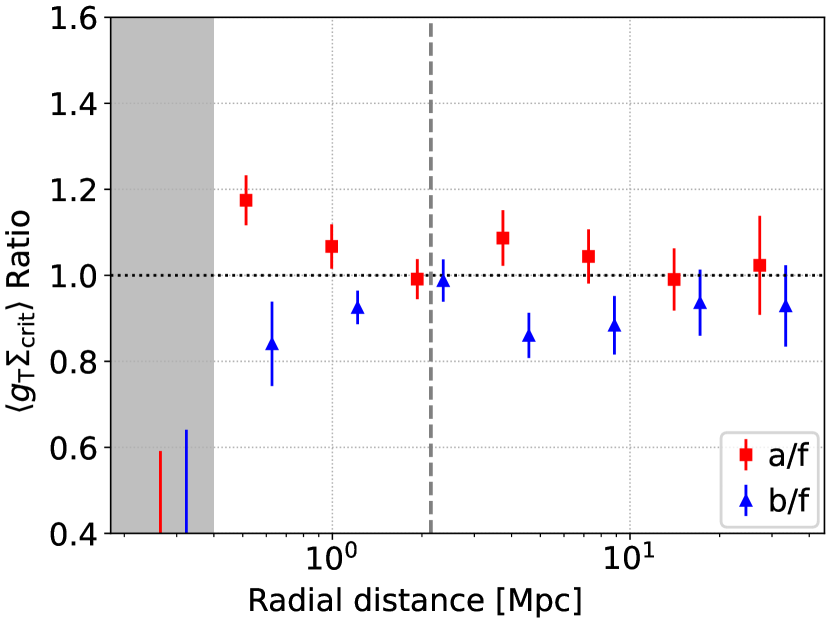
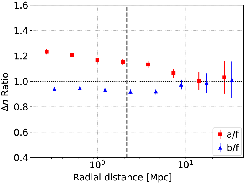
Figure 13: Normalized axis-aligned lensing profiles (left) and excess number density profiles (right) using a sample of LS clusters that are nearly relaxed. The shapes and photometry are still from DES Y3 and DES DR2. The lensing analysis includes 13147 clusters for the fiducial and 11813 clusters for the $a,b$ subsamples, while the number density analysis includes 13310 and 11817 clusters respectively.

Appendix B Individual richness/redshift bins for excess number density ratio

We divide the cluster sample into four subsamples by both redshift and richness, which both have two bins, and stack the excess galaxy number density in each bin to compute respective normalized profiles (Figure 14). The result is much noisier than the one in the main text, which uses two bins for redshift or richness only (Figure 7; Section 4.4). We test the same $2\times 2$ binning for the lensing data and find the result is even noiser. Therefore, in the main text we only use two bins rather than four bins to divide the cluster sample by redshift or richness.

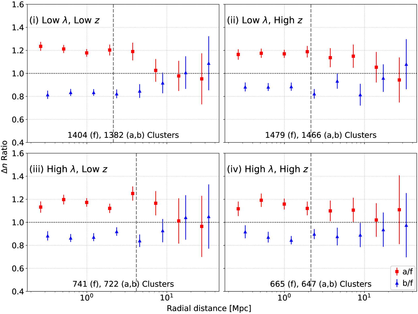
Figure 14: Normalized axis-aligned excess number density profiles in individual richness ($\lambda$) and redshift ($z$) bins. Note we decrease the jackknife region numbers to 72 and 64 for the high-$\lambda$ low-z and high-$\lambda$ high-z datasets respectively because of the limited number of clusters (others are using the default 100 regions). The low-richness low-redshift bin shows the smallest converging radius.

Appendix C Flow chart for the Pipeline

The flow chart (Figure 15) illustrates our pipeline – it starts from selecting a cluster sample and making queries for catalogues, then to computing the CG angle and selecting sources based on the angle, and to stacking the catalogues, and finally to producing the stacked profiles and their ratios.

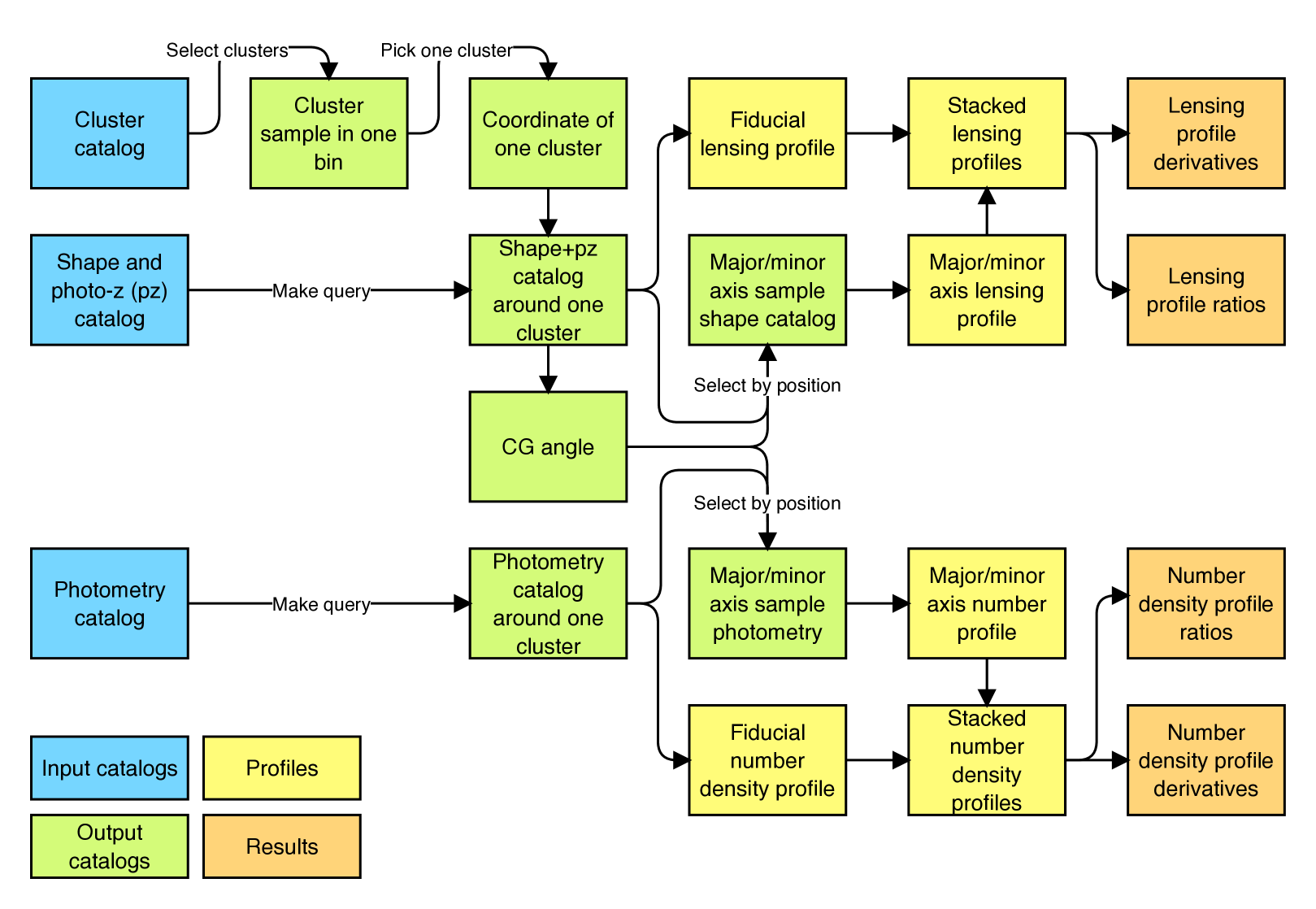
Figure 15: Flower chart of our pipeline. We note that obtaining a CG angle do not require photo-z information, and thus CGs can be queried independently using small cone searches. Further cuts can be made on the photometry catalogues, e.g. a red-sequence cut (Section 4.5).

References

- Abbott et al. (2018) Abbott T. M. C., et al., 2018, ApJS, 239, 18
- Abbott et al. (2020) Abbott T. M. C., et al., 2020, Phys. Rev. D, 102, 023509
- Abbott et al. (2021) Abbott T. M. C., et al., 2021, ApJS, 255, 20
- Aihara et al. (2019) Aihara H., et al., 2019, PASJ, 71, 114
- Allen et al. (2011) Allen S. W., Evrard A. E., Mantz A. B., 2011, ARA&A, 49, 409
- Astropy Collaboration et al. (2013) Astropy Collaboration et al., 2013, A&A, 558, A33
- Astropy Collaboration et al. (2018) Astropy Collaboration et al., 2018, AJ, 156, 123
- Bartelmann & Schneider (2001) Bartelmann M., Schneider P., 2001, Phys. Rep., 340, 291
- Baxter et al. (2017) Baxter E., et al., 2017, ApJ, 841, 18
- Becker & Kravtsov (2011) Becker M. R., Kravtsov A. V., 2011, ApJ, 740, 25
- Bertin & Arnouts (1996) Bertin E., Arnouts S., 1996, A&AS, 117, 393
- Bleem et al. (2020) Bleem L. E., et al., 2020, ApJS, 247, 25
- Bocquet et al. (2019) Bocquet S., et al., 2019, ApJ, 878, 55
- Breiman (2001) Breiman L., 2001, Machine learning, 45, 5
- Chang et al. (2018) Chang C., et al., 2018, ApJ, 864, 83
- Chen et al. (2019) Chen H., Avestruz C., Kravtsov A. V., Lau E. T., Nagai D., 2019, MNRAS, 490, 2380
- Child et al. (2018) Child H. L., Habib S., Heitmann K., Frontiere N., Finkel H., Pope A., Morozov V., 2018, ApJ, 859, 55
- Clampitt & Jain (2016) Clampitt J., Jain B., 2016, MNRAS, 457, 4135
- Coil (2013) Coil A. L., 2013, in Oswalt T. D., Keel W. C., eds, , Vol. 6, Planets, Stars and Stellar Systems. Volume 6: Extragalactic Astronomy and Cosmology. p. 387, doi:10.1007/978-94-007-5609-0_8
- Costanzi et al. (2019) Costanzi M., et al., 2019, MNRAS, 488, 4779
- Costanzi et al. (2021) Costanzi M., et al., 2021, Phys. Rev. D, 103, 043522
- De Luca et al. (2021) De Luca F., De Petris M., Yepes G., Cui W., Knebe A., Rasia E., 2021, MNRAS, 504, 5383
- De Vicente et al. (2016) De Vicente J., Sánchez E., Sevilla-Noarbe I., 2016, MNRAS, 459, 3078
- Despali et al. (2014) Despali G., Giocoli C., Tormen G., 2014, MNRAS, 443, 3208
- Dey et al. (2019) Dey A., et al., 2019, AJ, 157, 168
- Diemer & Kravtsov (2014) Diemer B., Kravtsov A. V., 2014, ApJ, 789, 1
- Dodelson et al. (2016) Dodelson S., Heitmann K., Hirata C., Honscheid K., Roodman A., Seljak U., Slosar A., Trodden M., 2016, arXiv e-prints, p. arXiv:1604.07626
- Donahue et al. (2016) Donahue M., et al., 2016, ApJ, 819, 36
- Farahi et al. (2022) Farahi A., Nagai D., Anbajagane D., 2022, ApJ, 933, 48
- Gatti et al. (2021) Gatti M., et al., 2021, MNRAS, 504, 4312
- Gonzalez et al. (2021) Gonzalez E. J., Ragone-Figueroa C., Donzelli C. J., Makler M., García Lambas D., Granato G. L., 2021, MNRAS, 508, 1280
- Górski et al. (2005) Górski K. M., Hivon E., Banday A. J., Wandelt B. D., Hansen F. K., Reinecke M., Bartelmann M., 2005, ApJ, 622, 759
- Gouin et al. (2020) Gouin C., Aghanim N., Bonjean V., Douspis M., 2020, A&A, 635, A195
- Harris et al. (2020) Harris C. R., et al., 2020, Nature, 585, 357
- Herbonnet et al. (2019) Herbonnet R., von der Linden A., Allen S. W., Mantz A. B., Modumudi P., Morris R. G., Kelly P. L., 2019, MNRAS, 490, 4889
- Herbonnet et al. (2022) Herbonnet R., et al., 2022, MNRAS, 513, 2178
- Hoyle et al. (2018) Hoyle B., et al., 2018, MNRAS, 478, 592
- Huff & Mandelbaum (2017) Huff E., Mandelbaum R., 2017, arXiv e-prints, p. arXiv:1702.02600
- Hunter (2007) Hunter J. D., 2007, Computing in Science and Engineering, 9, 90
- Jarvis et al. (2021) Jarvis M., et al., 2021, MNRAS, 501, 1282
- Kasun & Evrard (2005) Kasun S. F., Evrard A. E., 2005, ApJ, 629, 781
- Kauffmann et al. (1997) Kauffmann G., Nusser A., Steinmetz M., 1997, MNRAS, 286, 795
- Kitayama et al. (2023) Kitayama T., et al., 2023, PASJ, 75, 311
- Knebe & Wießner (2006) Knebe A., Wießner V., 2006, Publ. Astron. Soc. Australia, 23, 125
- Kovacs et al. (2022) Kovacs E., et al., 2022, The Open Journal of Astrophysics, 5, 1
- Kravtsov & Borgani (2012) Kravtsov A. V., Borgani S., 2012, ARA&A, 50, 353
- Lang et al. (2016) Lang D., Hogg D. W., Mykytyn D., 2016, The Tractor: Probabilistic astronomical source detection and measurement, Astrophysics Source Code Library, record ascl:1604.008 (ascl:1604.008)
- Lokken et al. (2022) Lokken M., et al., 2022, ApJ, 933, 134
- MacCrann et al. (2022) MacCrann N., et al., 2022, MNRAS, 509, 3371
- Machado Poletti Valle et al. (2021) Machado Poletti Valle L. F., Avestruz C., Barnes D. J., Farahi A., Lau E. T., Nagai D., 2021, MNRAS, 507, 1468
- Mantz et al. (2015a) Mantz A. B., et al., 2015a, MNRAS, 446, 2205
- Mantz et al. (2015b) Mantz A. B., Allen S. W., Morris R. G., Schmidt R. W., von der Linden A., Urban O., 2015b, MNRAS, 449, 199
- McClintock et al. (2019) McClintock T., et al., 2019, MNRAS, 482, 1352
- Melchior et al. (2017) Melchior P., et al., 2017, MNRAS, 469, 4899
- Mendoza et al. (2023) Mendoza I., Mansfield P., Wang K., Avestruz C., 2023, MNRAS,
- More et al. (2016) More S., et al., 2016, ApJ, 825, 39
- Morganson et al. (2018) Morganson E., et al., 2018, PASP, 130, 074501
- Mulroy et al. (2019) Mulroy S. L., et al., 2019, MNRAS, 484, 60
- Narayan & Bartelmann (1996) Narayan R., Bartelmann M., 1996, arXiv e-prints, pp astro–ph/9606001
- Navarro et al. (1996) Navarro J. F., Frenk C. S., White S. D. M., 1996, ApJ, 462, 563
- Noh & Cohn (2012) Noh Y., Cohn J. D., 2012, MNRAS, 426, 1829
- Norberg et al. (2009) Norberg P., Baugh C. M., Gaztañaga E., Croton D. J., 2009, MNRAS, 396, 19
- Oguri (2010) Oguri M., 2010, PASJ, 62, 1017
- Oguri et al. (2003) Oguri M., Lee J., Suto Y., 2003, ApJ, 599, 7
- Oguri et al. (2010) Oguri M., Takada M., Okabe N., Smith G. P., 2010, MNRAS, 405, 2215
- Oke & Gunn (1983) Oke J. B., Gunn J. E., 1983, ApJ, 266, 713
- Osato et al. (2018) Osato K., Nishimichi T., Oguri M., Takada M., Okumura T., 2018, MNRAS, 477, 2141
- Park et al. (2023) Park Y., Sunayama T., Takada M., Kobayashi Y., Miyatake H., More S., Nishimichi T., Sugiyama S., 2023, MNRAS, 518, 5171
- Perez & Granger (2007) Perez F., Granger B. E., 2007, Computing in Science and Engineering, 9, 21
- Phriksee et al. (2020) Phriksee A., Jullo E., Limousin M., Shan H., Finoguenov A., Komonjinda S., Wannawichian S., Sawangwit U., 2020, MNRAS, 491, 1643
- Rasia et al. (2013) Rasia E., Meneghetti M., Ettori S., 2013, The Astronomical Review, 8, 40
- Rodríguez-Gonzálvez et al. (2017) Rodríguez-Gonzálvez C., Chary R. R., Muchovej S., Melin J. B., Feroz F., Olamaie M., Shimwell T., 2017, MNRAS, 464, 2378
- Rozo & Rykoff (2014) Rozo E., Rykoff E. S., 2014, ApJ, 783, 80
- Rozo et al. (2015a) Rozo E., Rykoff E. S., Bartlett J. G., Melin J.-B., 2015a, MNRAS, 450, 592
- Rozo et al. (2015b) Rozo E., Rykoff E. S., Becker M., Reddick R. M., Wechsler R. H., 2015b, MNRAS, 453, 38
- Rykoff et al. (2014) Rykoff E. S., et al., 2014, ApJ, 785, 104
- Rykoff et al. (2016) Rykoff E. S., et al., 2016, ApJS, 224, 1
- Schneider (2005) Schneider P., 2005, arXiv e-prints, pp astro–ph/0509252
- Schramm (1990) Schramm T., 1990, A&A, 231, 19
- Sereno et al. (2021) Sereno M., Lovisari L., Cui W., Schellenberger G., 2021, MNRAS, 507, 5214
- Sevilla et al. (2011) Sevilla I., et al., 2011, arXiv e-prints, p. arXiv:1109.6741
- Sheldon & Huff (2017) Sheldon E. S., Huff E. M., 2017, ApJ, 841, 24
- Sheldon et al. (2004) Sheldon E. S., et al., 2004, AJ, 127, 2544
- Shin et al. (2018) Shin T.-h., Clampitt J., Jain B., Bernstein G., Neil A., Rozo E., Rykoff E., 2018, MNRAS, 475, 2421
- Shin et al. (2019) Shin T., et al., 2019, MNRAS, 487, 2900
- Sifón et al. (2015) Sifón C., Hoekstra H., Cacciato M., Viola M., Köhlinger F., van der Burg R. F. J., Sand D. J., Graham M. L., 2015, A&A, 575, A48
- Sunayama & More (2019) Sunayama T., More S., 2019, MNRAS, 490, 4945
- Tempel et al. (2015) Tempel E., Guo Q., Kipper R., Libeskind N. I., 2015, MNRAS, 450, 2727
- Vallés-Pérez et al. (2023) Vallés-Pérez D., Planelles S., Monllor-Berbegal Ó., Quilis V., 2023, MNRAS, 519, 6111
- Varga et al. (2019) Varga T. N., et al., 2019, MNRAS, 489, 2511
- Vikhlinin et al. (2009) Vikhlinin A., et al., 2009, ApJ, 692, 1060
- Virtanen et al. (2020) Virtanen P., et al., 2020, Nature Methods, 17, 261
- Wu et al. (2022) Wu H.-Y., et al., 2022, MNRAS, 515, 4471
- Xhakaj et al. (2020) Xhakaj E., Diemer B., Leauthaud A., Wasserman A., Huang S., Luo Y., Adhikari S., Singh S., 2020, MNRAS, 499, 3534
- Yuan & Wen (2022) Yuan Z. S., Wen Z. L., 2022, MNRAS, 516, 3159
- Zhang & Annis (2022) Zhang Y., Annis J., 2022, MNRAS, 511, L30
- Zhang et al. (2013) Zhang Y., Dietrich J. P., McKay T. A., Sheldon E. S., Nguyen A. T. Q., 2013, ApJ, 773, 115
- Zhang et al. (2019) Zhang Y., et al., 2019, MNRAS, 487, 2578
- Zhang et al. (2023) Zhang Z., et al., 2023, MNRAS, 523, 1994
- Zhou et al. (2021) Zhou R., et al., 2021, MNRAS, 501, 3309
- Zonca et al. (2019) Zonca A., Singer L., Lenz D., Reinecke M., Rosset C., Hivon E., Gorski K., 2019, Journal of Open Source Software, 4, 1298
- Zou et al. (2021) Zou H., et al., 2021, ApJS, 253, 56
- Zu et al. (2021) Zu Y., et al., 2021, MNRAS, 505, 5117
- Zuntz et al. (2018) Zuntz J., et al., 2018, MNRAS, 481, 1149