Thermomechanics of ferri-antiferromagnetic phase transition in finitely-strained rocks
towards paleomagnetism

Abstract

The thermodynamic model of visco-elastic deformable magnetic materials at finite strains is formulated in a fully Eulerian way in rates with the aim to describe thermoremanent paleomagnetism in crustal rocks. The Landau theory applied to a ferro-to-para-magnetic phase transition, the gradient theory for magnetization (leading to exchange energy) with general mechanically dependent coefficient, hysteresis in magnetization evolution by Gilbert equation involving objective corotational time derivative of magnetization, and demagnetizing field are considered in the model. The Jeffreys viscoelastic rheology is used with temperature-dependent creep to model solidification or melting transition. The model complies with energy conservation and the Clausius-Duhem entropy inequality.

Keywords: deforming magnetic rock modelling, Landau magnetic phase transition, hysteretic Gilbert equation, large strains in Eulerian formulation, Jeffreys viscoelastic rheology, solidification/melting, rock-magma phase transition, thermoremanent paleomagnetism.

1 Introduction

Deformable magnetic media are an interesting multi-physical area of continuum mechanics. Applications to paleomagnetism in crustal rocks is particularly interesting because it combines sophisticated viscoelastic rheology with thermomechanics and with mechanical and magnetical phase transitions, i.e. liquid magma to essentially solid rocks and para- (or rather antiferro-) magnetism to ferro- (or rather ferri-) magnetism in rocks. Magnetism in (some) rocks forms a vital part of rock physics and mechanics, cf. [5, 6, 10, 21, 36]. Paleomagnetism refers to “frozen” magnetism in oceanic or continental rocks, which may give information about history of geomagnetic field generated in the Earth’s outer core or history of deformation of continental crust, respectively. Interestingly, paleomagnetism exists also in other planets that nowadays do not have substantial magnetic fields, specifically Mars and Mercury. Cf. [5] and [7] for a survey.

Some chemical components in rocks as iron oxides (as magnetite and hematite) and some other oxides (e.g. iron-titanium oxide in basalts) are ferrimagnetic in low temperatures. They form a single- or poly-crystalic grains in mostly nonmagnetic silicate rocks and can be magnetized by various mechanisms: Most important (which we are focused on) is thermoremanent magnetization in so-called igneous rocks which are formed through the cooling and solidification of magma or lava. and subsequent bending/folding of rocks in a constant geomagnetic field. The processes within gradual cooling and magnetization and subsequent deformation of rocks within long geological timescales are schematically depicted in Fig. 1; in fact, grains of magnetic minerals have randomly oriented easy-magnetization axes, some of them being magnetized more while others less. The other mechanisms are detrital remanent magnetization (in sediments), isothermal remanent magnetization (in strong magnetic fields typically during lightning at a fixed temperature), etc.

The deformation of rocks within long-time scales can surely be very large, both in the oceanic crust and in the continental crust, too. Thus large-strain setting is to be used. Here we will exploit the fully nonlinear continuum mechanics of magnetic materials as devised for isothermal situations by [8, 9]. Together with the anisothermal Landau phase-transition theory, applied for rigid magnets as by [29], it gives a full thermomechanical model of deformable magnetic continua in the solid-type Kelvin-Voigt rheology, as analyzed in a multipolar variant by [32]. This is here presented in Section 2. To model the fluidic character of hot rocks (magma) and long-time-scale deforming cold rocks and the solidification phase transition, we must use a suitable rheology of the Maxwell type. This combination is formulated in Section 3, together with specifying the energetics behind the system and notes about analytical justification in a multipolar variant involving higher-order dissipative terms. Eventually, in Section 4, the application to paleomagnetism is briefly specified.

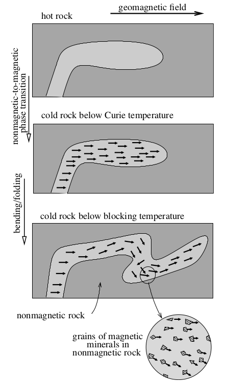
Figure 1: A schematic illustration of thermoremanent magnetization within cooling and deformation of magnetic rocks.

The main notation used below is summarized in Table 1.

Table 1: Nomenclature

${\boldsymbol{v}}$ velocity (in m/s),	${\boldsymbol{g}}$ gravity acceleration (in m/s2),
$\varrho$ mass density (in kg/m3),	${\boldsymbol{e}}({\boldsymbol{v}})$ small strain rate (in s-1),
${\boldsymbol{F}}$ deformation gradient,	${\mathbb{D}}$ viscosity-coefficient tensor,
${\boldsymbol{F}}_{\text{\!\rm e\,}}$ elastic distortion,	$\psi$ free energy (in Pa=J/m3),
${\boldsymbol{F}}_{\text{\!\rm i\,}}$ inelastic (creep) distortion,​​​	$\zeta$ dissipation potential (in Pa/s),​​
${\boldsymbol{L}}$ inelastic distortion rate,	$c$ heat capacity (in Pa/K),
${\boldsymbol{m}}$ magnetization (in A/m),	$k$ heat conductivity,
$\theta$ temperature (in K),	$\kappa$ exchange coefficient,
$u$ demagnetizing potential,	$\eta$ entropy (in Pa/K),
$\mu_{0}$ vaccum permeability,	${\boldsymbol{h}}$ total magnetic field (in A/m),
${\boldsymbol{T}}$ elastic Cauchy stress,	$\>{\boldsymbol{h}}_{\rm ext}$ external magnetic field,
${\boldsymbol{K}}$ Korteweg-like stress,	$\>\gamma$ gyromagnetic ratio,
$\SS$ magnetic-dipole stress,	$(^{{}_{{}_{\bullet}}})\!\mathchoice{{\buildrel\hskip 1.00006pt\text{\LARGE.}\over{}}}{{\buildrel\hskip 1.00006pt\text{\LARGE.}\over{}}}{{\buildrel\hskip 1.00006pt\text{\Large.}\over{}}}{{\buildrel\hskip 1.00006pt\text{\large.}\over{}}}$ convective time derivative,
$\mathscr{S}$ couple stress (in Pa m),	$\!(^{{}_{{}_{\bullet}}})\!\mathchoice{{\buildrel\hskip 1.00006pt{{}_{{}_{\Large\boldsymbol{\circ}}}}\over{}}}{{\buildrel\hskip 1.00006pt{{}_{{}_{\Large\boldsymbol{\circ}}}}\over{}}}{{\buildrel\hskip 1.00006pt{{}_{{}_{\Large\boldsymbol{\circ}}}}\over{}}}{{\buildrel\hskip 1.00006pt{\boldsymbol{\circ}}\over{}}}$corotational time derivative.​​

2 Viscoelastic finitely
strained magnets

The basic bricks for building our magneto-thermo-viscoelastic model are continuum mechanics, Landau’s theory of phase transition applied to magnetism in deforming media, and thermomechanics.

2.1 Eulerian continuum mechanics

The basic kinematic concept is the time-evolving deformation ${\boldsymbol{y}}:\varOmega\to\mathbb{R}^{3}$ as a mapping from a reference configuration of the body $\varOmega\subset\mathbb{R}^{3}$ into a physical space $\mathbb{R}^{3}$. The “Lagrangian” space variable in the reference configuration will be denoted as ${\boldsymbol{X}}\in\varOmega$ while in the “Eulerian” physical-space variable by ${\boldsymbol{x}}\in\mathbb{R}^{3}$. The basic kinematic and geometrical objects are the Lagrangian velocity ${\boldsymbol{v}}=\frac{\partial{}}{\partial t}{\boldsymbol{y}}$ and the Lagrangian deformation gradient ${\nabla}_{\!{\boldsymbol{X}}}{\boldsymbol{y}}$.

Time evolving deformations ${\boldsymbol{x}}={\boldsymbol{y}}(t,{\boldsymbol{X}})$ are sometimes called “motions”. Further, assuming for a moment that ${\boldsymbol{y}}(t,\cdot)$ is invertible, we define the so-called return (sometimes called also a reference) mapping $\boldsymbol{\xi}:{\boldsymbol{x}}\mapsto{\boldsymbol{y}}^{-1}(t,{\boldsymbol{x}})$. The important quantities are the Eulerian velocity ${\boldsymbol{v}}(t,{\boldsymbol{x}})={\boldsymbol{v}}(t,\boldsymbol{\xi}(t,{\boldsymbol{x}}))$ and the Eulerian deformation gradient ${\boldsymbol{F}}(t,{\boldsymbol{x}})=[{\nabla}_{\!{\boldsymbol{X}}}{\boldsymbol{y}}](t,\boldsymbol{\xi}(t,{\boldsymbol{x}}))$. We use the dot-notation $(\cdot)\!\mathchoice{{\buildrel\hskip 1.00006pt\text{\LARGE.}\over{}}}{{\buildrel\hskip 1.00006pt\text{\LARGE.}\over{}}}{{\buildrel\hskip 1.00006pt\text{\Large.}\over{}}}{{\buildrel\hskip 1.00006pt\text{\large.}\over{}}}=\frac{\partial{}}{\partial t}+{\boldsymbol{v}}{\cdot}\nabla_{\boldsymbol{x}}$ for the convective time derivative applied to scalars or, component-wise, to vectors or tensors. Then the velocity gradient ${\nabla}{\boldsymbol{v}}=\nabla_{\!{\boldsymbol{X}}}{\boldsymbol{v}}\nabla_{\!{\boldsymbol{x}}}{\boldsymbol{X}}=\mathchoice{{\buildrel\hskip 1.00006pt\text{\LARGE.}\over{{\boldsymbol{F}}}}}{{\buildrel\hskip 1.00006pt\text{\LARGE.}\over{{\boldsymbol{F}}}}}{{\buildrel\hskip 1.00006pt\text{\Large.}\over{{\boldsymbol{F}}}}}{{\buildrel\hskip 1.00006pt\text{\large.}\over{{\boldsymbol{F}}}}}{\boldsymbol{F}}^{-1}$, where we used the chain-rule calculus and ${\boldsymbol{F}}^{-1}=(\nabla_{\!{\boldsymbol{X}}}{\boldsymbol{x}})^{-1}=\nabla_{\!{\boldsymbol{x}}}{\boldsymbol{X}}$. This gives the transport equation-and-evolution for the deformation gradient as

$$\mathchoice{{\buildrel\hskip 1.00006pt\text{\LARGE.}\over{{\boldsymbol{F}}}}}{{\buildrel\hskip 1.00006pt\text{\LARGE.}\over{{\boldsymbol{F}}}}}{{\buildrel\hskip 1.00006pt\text{\Large.}\over{{\boldsymbol{F}}}}}{{\buildrel\hskip 1.00006pt\text{\large.}\over{{\boldsymbol{F}}}}}=(\nabla{\boldsymbol{v}}){\boldsymbol{F}}\,.$$ (2.1)

The return mapping $\boldsymbol{\xi}$ satisfies the transport equation

$$\mathchoice{{\buildrel\hskip 1.00006pt\text{\LARGE.}\over{\boldsymbol{\xi}}}}{{\buildrel\hskip 1.00006pt\text{\LARGE.}\over{\boldsymbol{\xi}}}}{{\buildrel\hskip 1.00006pt\text{\Large.}\over{\boldsymbol{\xi}}}}{{\buildrel\hskip 1.00006pt\text{\large.}\over{\boldsymbol{\xi}}}}=\boldsymbol{0}\,;$$ (2.2)

note that, since we confined ourselves to a spatially homogeneous material (except Remark 4.1 below), actually $\boldsymbol{\xi}$ does not explicitly occur in the formulation of the problem, although we could use it while substituting ${\boldsymbol{F}}=(\nabla\boldsymbol{\xi})^{-1}$.

2.2 Free energy and dissipation potential

Beside the mechanical variables in Section 2.1, we consider the magnetization vector field ${\boldsymbol{m}}$ and temperature $\theta$. The main ingredients of the model are the (volumetric) free energy $\psi=\psi({\boldsymbol{F}},{\boldsymbol{m}},\theta)$ considered per the referential volume (so at this point ${\boldsymbol{F}}$ and ${\boldsymbol{m}}$ and $\theta$ are meant only as placeholders where later the actually fields are placed) and mechanical and magnetic dissipative-forces. It should be noted that such free energy (considered in J/m³=Pa) correspond to “standard” physical data while the actual free energy (considered also in J/m³=Pa) is $\psi({\boldsymbol{F}},{\boldsymbol{m}},\theta)/\!\det{\boldsymbol{F}}$. Let us remark that an alternative referential energy $\psi$ could be (and sometimes is) considered in J/kg so that than the actual energy wold be $\varrho\psi$. In any case, the actual free energy acts on the actual (i.e. Eulerian) deformation gradient ${\boldsymbol{F}}$, actual magnetization ${\boldsymbol{m}}$, and actual temperature $\theta$ as functions of the Eulerian ${\boldsymbol{x}}$ and of time $t$.

In addition, it is conventional in micromagnetism (cf. e.g. [4]) to augment the free energy also by an exchange energy $\upkappa({\boldsymbol{F}})|\nabla{\boldsymbol{m}}|^{2}$. The free energy considered per actual (not referential) volume extended by the Zeeman energy arising by an applied external actual (not referential) magnetic field ${\boldsymbol{h}}_{\rm ext}$, i.e. the Gibbs-type actual free energy, is thus

$$\psi_{\text{\sc g}}(t;{\boldsymbol{F}},{\boldsymbol{m}},\nabla{\boldsymbol{m}},\theta) =\!\!\!\!\!\begin{array}[t]{c}\begin{array}[t]{c}\underbrace{\frac{\psi({\boldsymbol{F}},{\boldsymbol{m}},\theta)}{\det{\boldsymbol{F}}}}\vspace*{.5em}\end{array}\vspace*{-1em}\\ _{\mbox{\footnotesize\rm actual free energy}}\end{array}\!\!\!\!\!\!$$ (2.6)

$$\hskip 6.99997pt-\!\!\!\!\!\!\begin{array}[t]{c}\begin{array}[t]{c}\underbrace{\mu_{0}{\boldsymbol{h}}_{\rm ext}(t){\cdot}{\boldsymbol{m}}}\vspace*{.5em}\end{array}\vspace*{-1em}\\ _{\mbox{\footnotesize\rm Zeeman}}\vspace*{-.5em}\\ _{\mbox{\footnotesize\rm energy}}\end{array}\!\!\!\!\!\!\!+\!\!\!\!\!\!\begin{array}[t]{c}\begin{array}[t]{c}\underbrace{\frac{\upkappa({\boldsymbol{F}})|\nabla{\boldsymbol{m}}|^{2}}{2\det{\boldsymbol{F}}}}\vspace*{.5em}\end{array}\vspace*{-1em}\\ _{\mbox{\footnotesize\rm exchange}}\vspace*{-.5em}\\ _{\mbox{\footnotesize\rm energy}}\end{array}\!\!\!\!\!$$ (2.15)

with the coefficient $\upkappa$ depending generally on ${\boldsymbol{F}}$.

From the free energy (2.15), we can read as partial (functional) derivatives of $\psi$ with respect to ${\boldsymbol{F}}$, $\nabla{\boldsymbol{m}}$, ${\boldsymbol{m}}$, and $\theta$ respectively the conservative part of the Cauchy stress ${\boldsymbol{T}}$, a capillarity-like stress ${\boldsymbol{K}}$, the actual conservative magnetic driving force ${\boldsymbol{t}}$, and the entropy $\eta$ as:

$${\boldsymbol{T}}=\frac{[\psi_{\rm G}]_{\boldsymbol{F}}^{\prime}({\boldsymbol{F}},{\boldsymbol{m}},\nabla{\boldsymbol{m}},\theta){\boldsymbol{F}}^{\top}\!\!\!}{\det{\boldsymbol{F}}}$$

$$=\bigg{(}\!\psi_{\boldsymbol{F}}^{\prime}({\boldsymbol{F}},{\boldsymbol{m}},\theta)+\frac{\upkappa^{\prime}({\boldsymbol{F}})|\nabla{\boldsymbol{m}}|^{2}\!}{2}\;\bigg{)}\frac{{\boldsymbol{F}}^{\top}}{\det{\boldsymbol{F}}}\,,$$ (2.16a)

$${\boldsymbol{K}}=\frac{(\nabla{\boldsymbol{m}})^{\top}\psi_{\nabla{\boldsymbol{m}}}^{\prime}({\boldsymbol{F}},\nabla{\boldsymbol{m}})}{\det{\boldsymbol{F}}}=\mu_{0}\upkappa({\boldsymbol{F}})\frac{\nabla{\boldsymbol{m}}{\otimes}\nabla{\boldsymbol{m}}}{\det{\boldsymbol{F}}}\,,$$ (2.16b)

$${\boldsymbol{t}}=\frac{[\psi_{\rm G}]_{\boldsymbol{m}}^{\prime}({\boldsymbol{F}},{\boldsymbol{m}},\theta)}{\det{\boldsymbol{F}}}-{\rm div}\frac{[\psi_{\rm G}]_{\nabla{\boldsymbol{m}}}^{\prime}({\boldsymbol{F}},\nabla{\boldsymbol{m}})}{\det{\boldsymbol{F}}}-\mu_{0}{\boldsymbol{h}}_{\rm ext}$$

$$\ \ =\frac{\psi_{\boldsymbol{m}}^{\prime}({\boldsymbol{F}},{\boldsymbol{m}},\theta)\!\!}{\det{\boldsymbol{F}}}-{\rm div}\Big{(}\frac{\upkappa({\boldsymbol{F}})\nabla{\boldsymbol{m}}}{\det{\boldsymbol{F}}}\Big{)}-\mu_{0}{\boldsymbol{h}}_{\rm ext}\,,\ \text{ and}$$ (2.16c)

$$\eta=-\frac{\psi_{\theta}^{\prime}({\boldsymbol{F}},{\boldsymbol{m}},\theta)}{\det{\boldsymbol{F}}}\,.$$ (2.16d)

The product $\nabla{\boldsymbol{m}}{\otimes}\nabla{\boldsymbol{m}}$ in (2.16b) is to be understood componentwise, specifically $[\nabla{\boldsymbol{m}}{\otimes}\nabla{\boldsymbol{m}}]_{ij}$ $=\sum_{k=1}^{3}\frac{\partial}{\partial x_{i}}m_{k}\frac{\partial}{\partial x_{j}}m_{k}$ with ${\boldsymbol{m}}=(m_{1},m_{2},m_{3})$ and ${\boldsymbol{x}}=(x_{1},x_{2},x_{3})$.

The other mentioned ingredient of our model is dissipative forces. It is conventional (although not necessary) to read them from the mentioned dissipative-force potential $\zeta=\zeta(\theta;{\boldsymbol{e}},{\boldsymbol{r}})$ with ${\boldsymbol{e}}={\boldsymbol{e}}({\boldsymbol{v}})=\frac{1}{2}{\nabla}{\boldsymbol{v}}^{\top}\!+\frac{1}{2}{\nabla}{\boldsymbol{v}}$ and with ${\boldsymbol{r}}$ the magnetization rate to be specified later in (2.22). This determines the mechanical dissipative stress ${\boldsymbol{D}}=\zeta_{{\boldsymbol{e}}}^{\prime}(\theta;{\boldsymbol{e}},{\boldsymbol{r}})$ and the magnetic dissipative force ${\boldsymbol{d}}=\zeta_{{\boldsymbol{r}}}^{\prime}(\theta;{\boldsymbol{e}},{\boldsymbol{r}})$.

The momentum equilibrium equation then balances the divergence of the total Cauchy stress with the inertial and gravity force:

$$\varrho\mathchoice{{\buildrel\hskip 1.00006pt\text{\LARGE.}\over{{\boldsymbol{v}}}}}{{\buildrel\hskip 1.00006pt\text{\LARGE.}\over{{\boldsymbol{v}}}}}{{\buildrel\hskip 1.00006pt\text{\Large.}\over{{\boldsymbol{v}}}}}{{\buildrel\hskip 1.00006pt\text{\large.}\over{{\boldsymbol{v}}}}}-{\rm div}\big{(}{\boldsymbol{T}}{+}{\boldsymbol{D}}{+}{\boldsymbol{T}}_{\!\rm mag}{-}\,{\rm div}\,\mathscr{S}\big{)}=\varrho{\boldsymbol{g}}+{\boldsymbol{f}}_{\!\rm mag}$$ (2.17)

with ${\boldsymbol{T}}$ from (2.16d). Moreover, ${\boldsymbol{T}}_{\!\rm mag}$ and ${\boldsymbol{f}}_{\!\rm mag}$ are the magnetic stress and the magnetic force which balance the energetics, specifically

$${\boldsymbol{T}}_{\!\rm mag}\!\!:={\boldsymbol{K}}+\SS\ \ \text{ and }\ \ {\boldsymbol{f}}_{\!\rm mag}\!\!:=\mu_{0}(\nabla{\boldsymbol{h}})^{\top}{\boldsymbol{m}}-\mu_{0}\nabla({\boldsymbol{h}}{\cdot}{\boldsymbol{m}})$$

where $\SS$ is the skew-symmetric magnetic-dipole stress while $\mathscr{S}$ will be a “magnetic exchange hyperstress”, specifically

$$\SS={\rm skw}\big{(}(\mu_{0}{\boldsymbol{h}}{-}\psi_{\boldsymbol{m}}^{\prime}({\boldsymbol{F}},{\boldsymbol{m}},\theta)/\!\det{\boldsymbol{F}}){\otimes}{\boldsymbol{m}}\big{)}\ \ \ \text{ and}$$

$$\mathscr{S}={\rm Skw}\big{(}{\boldsymbol{m}}{\otimes}[\psi_{\rm G}]_{\nabla{\boldsymbol{m}}}^{\prime}({\boldsymbol{F}},\nabla{\boldsymbol{m}})\big{)}=\frac{\!\upkappa({\boldsymbol{F}}){\rm Skw}({\boldsymbol{m}}{\otimes}\nabla{\boldsymbol{m}})\!}{\det{\boldsymbol{F}}}\,,$$

where the skew-symmetric part “Skw” of the 3rd-order tensor is defined as

$$\big{[}{\rm Skw}({\boldsymbol{m}}{\otimes}\nabla{\boldsymbol{m}})\big{]}_{ijk}:=\frac{1}{2}\Big{(}m_{i}\frac{\partial m_{j}}{\partial x_{k}}-m_{j}\frac{\partial m_{i}}{\partial x_{k}}\Big{)}\,.$$ (2.18)

The driving magnetic force ${\boldsymbol{t}}$ in (2.16c) enters the Gilbert equation (2.23) in the next section while the entropy $\eta$ in (2.16d) will be the departure point for the formulation of the heat equation in Sect. 2.4.

2.3 Landau theory of magnetic phase transition

L.D. [19] devised a pioneering theory of phase transitions. The essence is in a simple polynomial free energy that changes its convex-vs-nonconvex character smoothly within varying temperature. Here, the free energy being 4th-order polynomial in terms of the magnetization ${\boldsymbol{m}}$ reads as

$$\psi=\psi({\boldsymbol{m}},\theta)=a|{\boldsymbol{m}}|^{4}\!+b(\theta{-}\theta_{\text{\sc c}})|{\boldsymbol{m}}|^{2}\!+c\theta(1{-}{\rm ln}\theta)$$ (2.19)

with $\theta_{\text{\sc c}}>0$ the Curie (or Neél) transition temperature, $a,b>0$, and $c>0$ the heat capacity. Note that the function $\psi=\psi(\cdot,\theta)$ is convex for $\theta\geq\theta_{\text{\sc c}}$, while for $\theta<\theta_{\text{\sc c}}$ it is nonconvex. In static magnetically soft magnets, the magnetization minimizes the energy. Here the minimum of $\psi(\text{\footnotesize$\,\bullet\,$},\theta)$ is attained on the orbit $|{\boldsymbol{m}}|=m_{\text{\sc s}}(\theta)$ with the radius (called saturation or spontaneous magnetization)

$$m_{\text{\sc s}}(\theta)=\begin{cases}\sqrt{a(\theta_{\text{\sc c}}{-}\theta)/(2b)}&\text{if }\ 0\leq\theta\leq\theta_{\text{\sc c}},\\ 0&\text{if }\ \theta\geq\theta_{\text{\sc c}}\,,\end{cases}$$ (2.20)

cf. the middle line in Figure 3 below. Noteworthy, in the external magnetic field ${\boldsymbol{h}}_{\rm ext}$, the contribution in (2.15) leads to the (slight) violation of the so-called Heisenberg constraint $|{\boldsymbol{m}}|=m_{\text{\sc s}}(\theta)$, cf. Fig. 5.4 in [3]. This constraint is often considered non-realistically in mathematical literature dealing with isothermal ferromagnetic modelling and, among other drawbacks, would not allow for anisothermal extension.

In time-dependent situations, employing a magnetization rate ${\boldsymbol{r}}$, the evolution of ${\boldsymbol{m}}$ is conventionally governed by the Gilbert equation ${\boldsymbol{r}}/\gamma={\boldsymbol{m}}{\times}(\mu_{0}{\boldsymbol{h}}{-}{\boldsymbol{t}}{-}\alpha{\boldsymbol{r}})$ with $\alpha>0$ a viscous-like damping constant, $\gamma=\gamma({\boldsymbol{m}},\theta)$ a gyromagnetic ratio, ${\boldsymbol{h}}$ an effective magnetic field, and ${\boldsymbol{t}}$ a magnetic driving force from (2.16c). This can also be written in the Landau-Lifschitz form as ${\boldsymbol{r}}+\gamma{\boldsymbol{m}}{\times}(\mu_{0}{\boldsymbol{h}}{-}{\boldsymbol{t}})=-\lambda{\boldsymbol{m}}{\times}({\boldsymbol{m}}{\times}(\mu_{0}{\boldsymbol{h}}{-}{\boldsymbol{t}}))$ with a suitable $\lambda$. Assuming for a moment $|{\boldsymbol{m}}|$ constant, the Gilbert equation can be rewritten into a more convenient form $\alpha{\boldsymbol{r}}-({\boldsymbol{m}}{\times}{\boldsymbol{r}})/\gamma=\mu_{0}{\boldsymbol{h}}-{\boldsymbol{t}}$, cf. [35].

This simple linear damping corresponds to a quadratic dissipation potential $\zeta({\boldsymbol{r}})=\frac{1}{2}\alpha|{\boldsymbol{r}}|^{2}$ with $|\cdot|$ denoting the Euclidean norm on $\mathbb{R}^{3}$, reflecting that we have in mind an isotropic situation in polycrystalline magnetic rocks. In many applications and in particular in paleomagnetism, the magnetic evolution is an activated process due to pinning effects which need certain activation energy for movement micro-magnetic walls. This can be described by adding a dry-friction-type 1-homogeneous nonsmooth term into the dissipation potential $\zeta({\boldsymbol{r}})=\frac{1}{2}\alpha|{\boldsymbol{r}}|^{2}+h_{\text{\rm c}}|{\boldsymbol{r}}|$ with $h_{\text{\rm c}}=h_{\text{\rm c}}(\theta)$ a so-called coercive force. The magnetic dissipative force is then ${\boldsymbol{d}}=\zeta^{\prime}({\boldsymbol{r}})=\alpha{\boldsymbol{r}}+h_{\text{\rm c}}{\rm Dir}({\boldsymbol{r}})$ with “Dir” denoting the set-valued monotone “direction” mapping

$${\rm Dir}({\boldsymbol{r}})=\begin{cases}\{{\boldsymbol{r}}\in\mathbb{R}^{3};\ |{\boldsymbol{r}}|\leq 1\}&\text{if }{\boldsymbol{r}}={\boldsymbol{0}}\,,\\ \quad{\boldsymbol{r}}/|{\boldsymbol{r}}|&\text{if }{\boldsymbol{r}}\neq{\boldsymbol{0}}\,,\end{cases}$$ (2.21)

cf. [35]; let us note the corresponding dissipation rate is ${\boldsymbol{d}}{\cdot}{\boldsymbol{r}}=\alpha|{\boldsymbol{r}}|^{2}+h_{\text{\rm c}}|{\boldsymbol{r}}|$. This nonsmooth extension was proposed by [1] and [41] as a device to model properly a hysteretic response in magnetization of ferromagnets, modifying the Gilbert equation by augmenting suitably the effective magnetic field. Although the original [13] and the [20] equations are equivalent to each other, the resulting augmented equations are no longer mutually equivalent. This has been pointed out in [28], where the conceptual differences between the Gilbert and the Landau-Lifschitz formats have been elucidated.

In rigid magnets, simply ${\boldsymbol{r}}=\frac{\partial{}}{\partial t}{\boldsymbol{m}}$. Yet, in deforming media in Eulerian description, the partial time derivative $\frac{\partial{}}{\partial t}{\boldsymbol{m}}$ should be replaced by an objective time derivative. Here we use the Zaremba-Jaumann (corotational) time derivative $\mathchoice{{\buildrel\hskip 1.00006pt{{}_{{}_{\Large\boldsymbol{\circ}}}}\over{{\boldsymbol{m}}}}}{{\buildrel\hskip 1.00006pt{{}_{{}_{\Large\boldsymbol{\circ}}}}\over{{\boldsymbol{m}}}}}{{\buildrel\hskip 1.00006pt{{}_{{}_{\Large\boldsymbol{\circ}}}}\over{{\boldsymbol{m}}}}}{{\buildrel\hskip 1.00006pt{\boldsymbol{\circ}}\over{{\boldsymbol{m}}}}}$, defined as

$$\mathchoice{{\buildrel\hskip 1.00006pt{{}_{{}_{\Large\boldsymbol{\circ}}}}\over{{\boldsymbol{m}}}}}{{\buildrel\hskip 1.00006pt{{}_{{}_{\Large\boldsymbol{\circ}}}}\over{{\boldsymbol{m}}}}}{{\buildrel\hskip 1.00006pt{{}_{{}_{\Large\boldsymbol{\circ}}}}\over{{\boldsymbol{m}}}}}{{\buildrel\hskip 1.00006pt{\boldsymbol{\circ}}\over{{\boldsymbol{m}}}}}=\mathchoice{{\buildrel\hskip 1.00006pt\text{\LARGE.}\over{{\boldsymbol{m}}}}}{{\buildrel\hskip 1.00006pt\text{\LARGE.}\over{{\boldsymbol{m}}}}}{{\buildrel\hskip 1.00006pt\text{\Large.}\over{{\boldsymbol{m}}}}}{{\buildrel\hskip 1.00006pt\text{\large.}\over{{\boldsymbol{m}}}}}-{\rm skw}(\nabla{\boldsymbol{v}}){\boldsymbol{m}}\ \ \ \text{ with }\ \ \ \mathchoice{{\buildrel\hskip 1.00006pt\text{\LARGE.}\over{{\boldsymbol{m}}}}}{{\buildrel\hskip 1.00006pt\text{\LARGE.}\over{{\boldsymbol{m}}}}}{{\buildrel\hskip 1.00006pt\text{\Large.}\over{{\boldsymbol{m}}}}}{{\buildrel\hskip 1.00006pt\text{\large.}\over{{\boldsymbol{m}}}}}=\frac{\partial{{\boldsymbol{m}}}}{\partial t}+({\boldsymbol{v}}{\cdot}\nabla){\boldsymbol{m}}\,.$$ (2.22)

Thus, for ${\boldsymbol{r}}=\mathchoice{{\buildrel\hskip 1.00006pt{{}_{{}_{\Large\boldsymbol{\circ}}}}\over{{\boldsymbol{m}}}}}{{\buildrel\hskip 1.00006pt{{}_{{}_{\Large\boldsymbol{\circ}}}}\over{{\boldsymbol{m}}}}}{{\buildrel\hskip 1.00006pt{{}_{{}_{\Large\boldsymbol{\circ}}}}\over{{\boldsymbol{m}}}}}{{\buildrel\hskip 1.00006pt{\boldsymbol{\circ}}\over{{\boldsymbol{m}}}}}$, the Gilbert equation with dry friction turns into

$$\alpha\mathchoice{{\buildrel\hskip 1.00006pt{{}_{{}_{\Large\boldsymbol{\circ}}}}\over{{\boldsymbol{m}}}}}{{\buildrel\hskip 1.00006pt{{}_{{}_{\Large\boldsymbol{\circ}}}}\over{{\boldsymbol{m}}}}}{{\buildrel\hskip 1.00006pt{{}_{{}_{\Large\boldsymbol{\circ}}}}\over{{\boldsymbol{m}}}}}{{\buildrel\hskip 1.00006pt{\boldsymbol{\circ}}\over{{\boldsymbol{m}}}}}+h_{\text{\rm c}}(\theta){\rm Dir}(\mathchoice{{\buildrel\hskip 1.00006pt{{}_{{}_{\Large\boldsymbol{\circ}}}}\over{{\boldsymbol{m}}}}}{{\buildrel\hskip 1.00006pt{{}_{{}_{\Large\boldsymbol{\circ}}}}\over{{\boldsymbol{m}}}}}{{\buildrel\hskip 1.00006pt{{}_{{}_{\Large\boldsymbol{\circ}}}}\over{{\boldsymbol{m}}}}}{{\buildrel\hskip 1.00006pt{\boldsymbol{\circ}}\over{{\boldsymbol{m}}}}})-\frac{{\boldsymbol{m}}{\times}\mathchoice{{\buildrel\hskip 1.00006pt{{}_{{}_{\Large\boldsymbol{\circ}}}}\over{{\boldsymbol{m}}}}}{{\buildrel\hskip 1.00006pt{{}_{{}_{\Large\boldsymbol{\circ}}}}\over{{\boldsymbol{m}}}}}{{\buildrel\hskip 1.00006pt{{}_{{}_{\Large\boldsymbol{\circ}}}}\over{{\boldsymbol{m}}}}}{{\buildrel\hskip 1.00006pt{\boldsymbol{\circ}}\over{{\boldsymbol{m}}}}}}{\gamma({\boldsymbol{m}},\theta)}\ni\mu_{0}{\boldsymbol{h}}-{\boldsymbol{t}}\,,$$ (2.23)

the inclusion “$\ni$” being related to that the left-hand side is set-valued at the zero rate. Moreover, in a deforming continuum, we can consider a more general ${\boldsymbol{F}}$-dependent $\gamma=\gamma({\boldsymbol{F}},{\boldsymbol{m}},\theta)$ and $h_{\text{\rm c}}=h_{\text{\rm c}}({\boldsymbol{F}},\theta)$ but, rather due to notational simplicity, we will not explicitly consider it.

Let us emphasize that the convective derivative $\mathchoice{{\buildrel\hskip 1.00006pt\text{\LARGE.}\over{{\boldsymbol{m}}}}}{{\buildrel\hskip 1.00006pt\text{\LARGE.}\over{{\boldsymbol{m}}}}}{{\buildrel\hskip 1.00006pt\text{\Large.}\over{{\boldsymbol{m}}}}}{{\buildrel\hskip 1.00006pt\text{\large.}\over{{\boldsymbol{m}}}}}$ itself is not objective and would not be suitable in our context, except perhaps some laminar-like deformation as implicitly used in an incompressible isothermal variant by [2] or [42] or in a nanoparticle transport in fluids by [14].

In deformable (and deforming) magnetic media, the Zaremba-Jaumann corotational derivative for magnetization was suggested already by [23] to model situations when the magnetization can be “frozen” in hard-magnetic materials in their ferro- or ferri-magnetic state. For this effect, it is important the left-hand side in (2.23) contains the function “Dir” which is set-valued at $\mathchoice{{\buildrel\hskip 1.00006pt{{}_{{}_{\Large\boldsymbol{\circ}}}}\over{{\boldsymbol{m}}}}}{{\buildrel\hskip 1.00006pt{{}_{{}_{\Large\boldsymbol{\circ}}}}\over{{\boldsymbol{m}}}}}{{\buildrel\hskip 1.00006pt{{}_{{}_{\Large\boldsymbol{\circ}}}}\over{{\boldsymbol{m}}}}}{{\buildrel\hskip 1.00006pt{\boldsymbol{\circ}}\over{{\boldsymbol{m}}}}}=0$ so that for $h_{\rm c}$ large (which will occur below the so-called blocking temperature as depicted in Fig. 3 below), necessarily $\mathchoice{{\buildrel\hskip 1.00006pt{{}_{{}_{\Large\boldsymbol{\circ}}}}\over{{\boldsymbol{m}}}}}{{\buildrel\hskip 1.00006pt{{}_{{}_{\Large\boldsymbol{\circ}}}}\over{{\boldsymbol{m}}}}}{{\buildrel\hskip 1.00006pt{{}_{{}_{\Large\boldsymbol{\circ}}}}\over{{\boldsymbol{m}}}}}{{\buildrel\hskip 1.00006pt{\boldsymbol{\circ}}\over{{\boldsymbol{m}}}}}=0$ so that ${\boldsymbol{m}}$ exhibits the mentioned “frozen” effect. Later, the Zaremba-Jaumann derivative was used in [8, 9] in the linear viscosity (magnetic attenuation) $\alpha$-term.

The total magnetic field ${\boldsymbol{h}}$ in (2.23) is a difference of an external (given) magnetic field ${\boldsymbol{h}}_{\rm ext}$ and the demagnetizing field ${\boldsymbol{h}}_{\rm dem}$ self-induced by the magnetization itself. For geophysical applications in Sect. 4, the full Maxwell electromagnetic system is considered simplified to magnetostatics, considering slow evolution and neglecting in particular eddy currents and even confining ourselves on electrically non-conductive media. Then ${\boldsymbol{h}}_{\rm dem}=-\nabla u$ with $u$ denoting a scalar-valued potential solving the Poisson-type equation

$${\rm div}(\nabla u-\chi_{\varOmega}{\boldsymbol{m}})=0$$ (2.24)

considered (in the sense of distribution) on the whole Universe with $\chi_{\varOmega}=\chi_{\varOmega}({\boldsymbol{x}})=1$ on $\varOmega$ while $=0$ outside $\varOmega$. Fixing $u(\infty)=0$, in our 3-dimensional case, there is the explicit integral formula for $u$, see (2.48e) below.

2.4 Thermodynamics

The further ingredient of the model is the entropy equation for the entropy $\eta$ from (2.16d):

$$\frac{\partial{\eta}}{\partial t}+{\rm div}\big{(}{\boldsymbol{v}}\,\eta\big{)}=\frac{\xi-{\rm div}\,{\boldsymbol{j}}}{\theta}\ \ \ \ \text{ with }\ {\boldsymbol{j}}=-k\nabla\theta\,$$ (2.25)

and with $\xi=\xi({\boldsymbol{F}},\theta;{\boldsymbol{e}}({\boldsymbol{v}}),\mathchoice{{\buildrel\hskip 1.00006pt{{}_{{}_{\Large\boldsymbol{\circ}}}}\over{{\boldsymbol{m}}}}}{{\buildrel\hskip 1.00006pt{{}_{{}_{\Large\boldsymbol{\circ}}}}\over{{\boldsymbol{m}}}}}{{\buildrel\hskip 1.00006pt{{}_{{}_{\Large\boldsymbol{\circ}}}}\over{{\boldsymbol{m}}}}}{{\buildrel\hskip 1.00006pt{\boldsymbol{\circ}}\over{{\boldsymbol{m}}}}})$ denoting the heat production rate specified later in (2.48f) and ${\boldsymbol{j}}$ the heat flux governed by the Fourier law with the thermal conductivity $k=k({\boldsymbol{F}},\theta)$. In the thermo-mechanically isolated system with ${\boldsymbol{v}}{\cdot}{\boldsymbol{n}}=0$ and $\nabla\theta{\cdot}{\boldsymbol{n}}=0$ on the boundary $\varGamma$ of $\varOmega$, integrating (2.25) over $\varOmega$ and using Green formula gives the Clausius-Duhem inequality, i.e.

$$\frac{\mathrm{d}}{\mathrm{d}t}\int_{\varOmega}\eta\,\mathrm{d}{\boldsymbol{x}}=\int_{\varOmega}\!\!\!\!\!\!\!\!\!\begin{array}[t]{c}\begin{array}[t]{c}\underbrace{\frac{\xi}{\theta}+k\frac{|\nabla\theta|^{2}}{\theta^{2}}}\vspace*{.5em}\end{array}\vspace*{-1em}\\ _{\mbox{\footnotesize\rm entropy production rate}}\end{array}\!\!\!\!\!\!\!\!\!\!\!\mathrm{d}{\boldsymbol{x}}\geq 0\,.$$ (2.29)

i.e. (2.25) ensures the 2nd law of thermodynamics, saying that the total entropy in isolated systems is nondecreasing in time. Substituting $\eta$ from (2.16d) into (2.25) written in the form $\theta\mathchoice{{\buildrel\hskip 1.00006pt\text{\LARGE.}\over{\eta}}}{{\buildrel\hskip 1.00006pt\text{\LARGE.}\over{\eta}}}{{\buildrel\hskip 1.00006pt\text{\Large.}\over{\eta}}}{{\buildrel\hskip 1.00006pt\text{\large.}\over{\eta}}}=\xi-{\rm div}\,{\boldsymbol{j}}-\theta\eta{\rm div}\,{\boldsymbol{v}}$, we obtain

$$c\mathchoice{{\buildrel\hskip 1.00006pt\text{\LARGE.}\over{\theta}}}{{\buildrel\hskip 1.00006pt\text{\LARGE.}\over{\theta}}}{{\buildrel\hskip 1.00006pt\text{\Large.}\over{\theta}}}{{\buildrel\hskip 1.00006pt\text{\large.}\over{\theta}}}=\xi+\theta\frac{\psi_{{\boldsymbol{F}}\theta}^{\prime\prime}({\boldsymbol{F}},{\boldsymbol{m}},\theta)\!}{\det{\boldsymbol{F}}}{:}\mathchoice{{\buildrel\hskip 1.00006pt\text{\LARGE.}\over{{\boldsymbol{F}}}}}{{\buildrel\hskip 1.00006pt\text{\LARGE.}\over{{\boldsymbol{F}}}}}{{\buildrel\hskip 1.00006pt\text{\Large.}\over{{\boldsymbol{F}}}}}{{\buildrel\hskip 1.00006pt\text{\large.}\over{{\boldsymbol{F}}}}}+\theta\frac{\psi_{{\boldsymbol{m}}\theta}^{\prime\prime}({\boldsymbol{F}},{\boldsymbol{m}},\theta)\!}{\det{\boldsymbol{F}}}{\cdot}\mathchoice{{\buildrel\hskip 1.00006pt\text{\LARGE.}\over{{\boldsymbol{m}}}}}{{\buildrel\hskip 1.00006pt\text{\LARGE.}\over{{\boldsymbol{m}}}}}{{\buildrel\hskip 1.00006pt\text{\Large.}\over{{\boldsymbol{m}}}}}{{\buildrel\hskip 1.00006pt\text{\large.}\over{{\boldsymbol{m}}}}}-{\rm div}\,{\boldsymbol{j}}$$

$$\text{ with the heat capacity }\ c=-\theta\,\frac{\!\psi_{\theta\theta}^{\prime\prime}({\boldsymbol{F}},{\boldsymbol{m}},\theta)\!}{\det{\boldsymbol{F}}}\,,$$ (2.30)

which can be understood as the heat equation for the temperature $\theta$ as an intensive variable.

The referential internal energy is given by the Gibbs relation $\psi+\theta\eta$. In our Eulerian formulation, we will need rather the actual internal energy, which, because of (2.16d), equals here to

$$\begin{array}[t]{c}\begin{array}[t]{c}\underbrace{\frac{\psi-\theta\psi_{\theta}^{\prime}}{\det{\boldsymbol{F}}}}\vspace*{.5em}\end{array}\vspace*{-1em}\\ _{\mbox{\footnotesize\rm actual}}\vspace*{-.5em}\\ _{\mbox{\footnotesize\rm internal}}\vspace*{-.5em}\\ _{\mbox{\footnotesize\rm energy}}\end{array}\!\!\!\!\!=\!\!\!\!\!\begin{array}[t]{c}\begin{array}[t]{c}\underbrace{\frac{\psi({\boldsymbol{F}},{\boldsymbol{m}},0)}{\det{\boldsymbol{F}}}}\vspace*{.5em}\end{array}\vspace*{-1em}\\ _{\mbox{\footnotesize\rm actual stored}}\vspace*{-.5em}\\ _{\mbox{\footnotesize\rm energy}}\end{array}\!\!\!\!\!+\!\!\!\!\!\!\begin{array}[t]{c}\begin{array}[t]{c}\underbrace{\frac{\phi({\boldsymbol{F}},{\boldsymbol{m}},\theta){-}\theta\phi_{\theta}^{\prime}({\boldsymbol{F}},{\boldsymbol{m}},\theta)}{\det{\boldsymbol{F}}}}\vspace*{.5em}\end{array}\vspace*{-1em}\\ _{\mbox{\footnotesize\rm$=:\omega({\boldsymbol{F}},{\boldsymbol{m}},\theta)\>$ thermal part of}}\vspace*{-.5em}\\ _{\mbox{\footnotesize\rm the internal energy}}\end{array}$$ (2.44)

$$\text{with }\ \phi({\boldsymbol{F}},{\boldsymbol{m}},\theta)=\psi({\boldsymbol{F}},{\boldsymbol{m}},{\boldsymbol{F}})-\psi({\boldsymbol{F}},{\boldsymbol{m}},0)\,.$$ (2.45)

In terms of the thermal part of the internal energy $w=\omega({\boldsymbol{F}},{\boldsymbol{m}},\theta)$ as an extensive variable, the heat equation (2.30) can be written in the so-called enthalpy formulation:

$$\frac{\partial{w}}{\partial t}+{\rm div}({\boldsymbol{v}}w)=\xi-{\rm div}\,{\boldsymbol{j}}+\frac{\phi^{\prime}_{{\boldsymbol{F}}}({\boldsymbol{F}},{\boldsymbol{m}},\theta)\!}{\det{\boldsymbol{F}}}{:}\mathchoice{{\buildrel\hskip 1.00006pt\text{\LARGE.}\over{{\boldsymbol{F}}}}}{{\buildrel\hskip 1.00006pt\text{\LARGE.}\over{{\boldsymbol{F}}}}}{{\buildrel\hskip 1.00006pt\text{\Large.}\over{{\boldsymbol{F}}}}}{{\buildrel\hskip 1.00006pt\text{\large.}\over{{\boldsymbol{F}}}}}$$

$$+\frac{\phi^{\prime}_{{\boldsymbol{m}}}({\boldsymbol{F}},{\boldsymbol{m}},\theta)\!}{\det{\boldsymbol{F}}}{\cdot}\mathchoice{{\buildrel\hskip 1.00006pt\text{\LARGE.}\over{{\boldsymbol{m}}}}}{{\buildrel\hskip 1.00006pt\text{\LARGE.}\over{{\boldsymbol{m}}}}}{{\buildrel\hskip 1.00006pt\text{\Large.}\over{{\boldsymbol{m}}}}}{{\buildrel\hskip 1.00006pt\text{\large.}\over{{\boldsymbol{m}}}}}\hskip 10.00002pt\text{ with }\ \ w=\omega({\boldsymbol{F}},{\boldsymbol{m}},\theta)\,.$$ (2.46)

2.5 Thermodynamically coupled system

The overall system then merges the momentum equation (2.17), the hysteretic Gilbert equation (2.23) with the Poisson equation (2.24) for the demagnetizing field, the heat equation (2.46) together with the kinematic equation (2.1) and the usual continuity equation for mass density $\varrho$ transported as an extensive variable, cf. (2.48a) below. We consider a specific dissipation potential

$$\zeta(\theta;{\boldsymbol{e}},{\boldsymbol{r}})=\frac{1}{2}{\mathbb{D}}{\boldsymbol{e}}{:}{\boldsymbol{e}}+\frac{1}{2}\alpha|{\boldsymbol{r}}|^{2}+h_{\text{\rm c}}|{\boldsymbol{r}}|$$ (2.47)

with ${\mathbb{D}}$ a 4th-order symmetric tensor of elastic moduli. Altogether, we arrive to a system of six equations for $(\varrho,{\boldsymbol{v}},{\boldsymbol{F}},{\boldsymbol{m}},u,\theta)$:

$$\frac{\partial{\varrho}}{\partial t}=-\,{\rm div}(\varrho{\boldsymbol{v}})\,,$$ (2.48a)

$$\frac{\partial{}}{\partial t}(\varrho{\boldsymbol{v}})={\rm div}\Big{(}{\boldsymbol{T}}+{\boldsymbol{K}}+\SS-{\rm div}\mathscr{S}+{\mathbb{D}}{\boldsymbol{e}}({\boldsymbol{v}})-\varrho{\boldsymbol{v}}{\otimes}{\boldsymbol{v}}\Big{)}$$

$$\hskip 40.00006pt+\mu_{0}(\nabla{\boldsymbol{h}})^{\top}{\boldsymbol{m}}-\mu_{0}\nabla({\boldsymbol{h}}{\cdot}{\boldsymbol{m}})+\varrho{\boldsymbol{g}}$$

$$\text{with }\ \SS={\rm skw}\Big{(}\Big{(}\mu_{0}{\boldsymbol{h}}{-}\frac{\psi_{\boldsymbol{m}}^{\prime}({\boldsymbol{F}},{\boldsymbol{m}},\theta)\!}{\det{\boldsymbol{F}}}\Big{)}{\otimes}{\boldsymbol{m}}\Big{)}\,,$$

$$\hskip 10.00002pt\mathscr{S}=\frac{\kappa({\boldsymbol{F}})}{\det{\boldsymbol{F}}}{\rm Skw}\big{(}{\boldsymbol{m}}{\otimes}\nabla{\boldsymbol{m}}),\ \text{ and }\ \ \$$

$$\hskip 10.00002pt{\boldsymbol{h}}={\boldsymbol{h}}_{\rm ext}+\nabla u\ \ \text{ and \ ${\boldsymbol{T}},\,{\boldsymbol{K}}$\ from (\ref{driving-fields}a,b)}\,,\!\!\!\!$$ (2.48b)

$$\frac{\partial{{\boldsymbol{F}}}}{\partial t}=({\nabla}{\boldsymbol{v}}){\boldsymbol{F}}-({\boldsymbol{v}}{\cdot}\nabla){\boldsymbol{F}}\,,$$ (2.48c)

$$\alpha\mathchoice{{\buildrel\hskip 1.00006pt{{}_{{}_{\Large\boldsymbol{\circ}}}}\over{{\boldsymbol{m}}}}}{{\buildrel\hskip 1.00006pt{{}_{{}_{\Large\boldsymbol{\circ}}}}\over{{\boldsymbol{m}}}}}{{\buildrel\hskip 1.00006pt{{}_{{}_{\Large\boldsymbol{\circ}}}}\over{{\boldsymbol{m}}}}}{{\buildrel\hskip 1.00006pt{\boldsymbol{\circ}}\over{{\boldsymbol{m}}}}}+h_{\text{\rm c}}(\theta){\rm Dir}(\mathchoice{{\buildrel\hskip 1.00006pt{{}_{{}_{\Large\boldsymbol{\circ}}}}\over{{\boldsymbol{m}}}}}{{\buildrel\hskip 1.00006pt{{}_{{}_{\Large\boldsymbol{\circ}}}}\over{{\boldsymbol{m}}}}}{{\buildrel\hskip 1.00006pt{{}_{{}_{\Large\boldsymbol{\circ}}}}\over{{\boldsymbol{m}}}}}{{\buildrel\hskip 1.00006pt{\boldsymbol{\circ}}\over{{\boldsymbol{m}}}}})$$

$$-\frac{{\boldsymbol{m}}{\times}\mathchoice{{\buildrel\hskip 1.00006pt{{}_{{}_{\Large\boldsymbol{\circ}}}}\over{{\boldsymbol{m}}}}}{{\buildrel\hskip 1.00006pt{{}_{{}_{\Large\boldsymbol{\circ}}}}\over{{\boldsymbol{m}}}}}{{\buildrel\hskip 1.00006pt{{}_{{}_{\Large\boldsymbol{\circ}}}}\over{{\boldsymbol{m}}}}}{{\buildrel\hskip 1.00006pt{\boldsymbol{\circ}}\over{{\boldsymbol{m}}}}}}{\gamma({\boldsymbol{m}},\theta)}\ni\mu_{0}{\boldsymbol{h}}-{\boldsymbol{t}}\ \text{ with ${\boldsymbol{t}}$ from (\ref{driving-field})}\,,$$ (2.48d)

$$u({\boldsymbol{x}})=\frac{1}{4\uppi}\int_{\varOmega}\frac{(\widetilde{\boldsymbol{x}}{-}{\boldsymbol{x}}){\cdot}{\boldsymbol{m}}(\widetilde{\boldsymbol{x}})}{|\widetilde{\boldsymbol{x}}{-}{\boldsymbol{x}}|^{3}}\,\mathrm{d}\widetilde{\boldsymbol{x}}\ \ \ \text{ for }\ {\boldsymbol{x}}\in\varOmega\,,$$ (2.48e)

$$\frac{\partial{w}}{\partial t}=\xi({\boldsymbol{F}},\theta;{\boldsymbol{e}}({\boldsymbol{v}}),\mathchoice{{\buildrel\hskip 1.00006pt{{}_{{}_{\Large\boldsymbol{\circ}}}}\over{{\boldsymbol{m}}}}}{{\buildrel\hskip 1.00006pt{{}_{{}_{\Large\boldsymbol{\circ}}}}\over{{\boldsymbol{m}}}}}{{\buildrel\hskip 1.00006pt{{}_{{}_{\Large\boldsymbol{\circ}}}}\over{{\boldsymbol{m}}}}}{{\buildrel\hskip 1.00006pt{\boldsymbol{\circ}}\over{{\boldsymbol{m}}}}})+\frac{\phi^{\prime}_{{\boldsymbol{F}}}({\boldsymbol{F}},{\boldsymbol{m}},\theta){\boldsymbol{F}}^{\top}\!\!}{\det{\boldsymbol{F}}}{:}{\boldsymbol{e}}({\boldsymbol{v}})$$

$$\hskip 70.0001pt+\frac{\phi_{\boldsymbol{m}}^{\prime}({\boldsymbol{F}},{\boldsymbol{m}},\theta)}{\det{\boldsymbol{F}}}{\cdot}\mathchoice{{\buildrel\hskip 1.00006pt\text{\LARGE.}\over{{\boldsymbol{m}}}}}{{\buildrel\hskip 1.00006pt\text{\LARGE.}\over{{\boldsymbol{m}}}}}{{\buildrel\hskip 1.00006pt\text{\Large.}\over{{\boldsymbol{m}}}}}{{\buildrel\hskip 1.00006pt\text{\large.}\over{{\boldsymbol{m}}}}}-{\rm div}\big{(}{\boldsymbol{j}}{+}w{\boldsymbol{v}}\big{)}$$

$$\text{ with }\ \xi({\boldsymbol{F}},\theta;{\boldsymbol{e}},{\boldsymbol{r}})={\mathbb{D}}{\boldsymbol{e}}{:}{\boldsymbol{e}}+\mu_{0}\alpha|{\boldsymbol{r}}|^{2}+\mu_{0}h_{\text{\rm c}}(\theta)|{\boldsymbol{r}}|$$

$$\text{ and }\ {\boldsymbol{j}}=-k({\boldsymbol{F}},\theta)\nabla\theta\,,$$

$$\text{ and }\ w=\omega({\boldsymbol{F}},{\boldsymbol{m}},\theta)=\frac{\phi({\boldsymbol{F}},{\boldsymbol{m}},\theta)-\theta\phi_{\theta}^{\prime}({\boldsymbol{F}},{\boldsymbol{m}},\theta)}{\det{\boldsymbol{F}}}$$

$$\text{ with }\ \phi({\boldsymbol{F}},{\boldsymbol{m}},\theta)=\psi({\boldsymbol{F}},{\boldsymbol{m}},\theta)-\psi({\boldsymbol{F}},{\boldsymbol{m}},0).$$ (2.48f)

The skew-symmetric stress $\SS$ and couple-like hyperstress $\mathscr{S}$ come from the magnetic dipoles and from the exchange energy and balances the energetics, cf. Sect. 3.3 below and the calculations in [32]; for a similar skew-symmetric stress $\SS$ see [8, 9] while the skew-symmetric hyperstress $\mathscr{S}$ is like in the Cosserat theory by [39]. The skew-symmetric couple-like hyperstress $\mathscr{S}$ balances the energetic as (3.45)–(3.76) below, being related with the corotation derivative $\mathchoice{{\buildrel\hskip 1.00006pt{{}_{{}_{\Large\boldsymbol{\circ}}}}\over{{\boldsymbol{m}}}}}{{\buildrel\hskip 1.00006pt{{}_{{}_{\Large\boldsymbol{\circ}}}}\over{{\boldsymbol{m}}}}}{{\buildrel\hskip 1.00006pt{{}_{{}_{\Large\boldsymbol{\circ}}}}\over{{\boldsymbol{m}}}}}{{\buildrel\hskip 1.00006pt{\boldsymbol{\circ}}\over{{\boldsymbol{m}}}}}$ used in (2.48d) and would not be visible if only the convective derivative $\mathchoice{{\buildrel\hskip 1.00006pt\text{\LARGE.}\over{{\boldsymbol{m}}}}}{{\buildrel\hskip 1.00006pt\text{\LARGE.}\over{{\boldsymbol{m}}}}}{{\buildrel\hskip 1.00006pt\text{\Large.}\over{{\boldsymbol{m}}}}}{{\buildrel\hskip 1.00006pt\text{\large.}\over{{\boldsymbol{m}}}}}$ were used there.

3 Creep and melting-solidification transition

The solid-type viscoelastic rheology in Section 2 has applications rather in metallic magnets but some other materials need rather more advanced rheologies, specifically some a fluidic-type rheology in the shear part of the model. This concerns, in particular, the geophysical application in Sect. 4 where very large displacements occur within long geological periods.

3.1 Creep in multiplicative decomposition

Our treatment of finite-strain inelasticity (here creep) will be based on the [18] and [22] multiplicative decomposition, as routinely used in plasticity, i.e.

$${\boldsymbol{F}}={\boldsymbol{F}}_{\text{\!\rm e\,}}{\boldsymbol{F}}_{\text{\!\rm i\,}}\,,$$ (3.1)

where ${\boldsymbol{F}}_{\text{\!\rm i\,}}$ is a inelastic distortion tensor. This tensor ${\boldsymbol{F}}_{\text{\!\rm i\,}}$ is interpreted as a transformation of the reference configuration into an intermediate stress-free configuration, which is then mapped into the current configuration by the elastic strain ${\boldsymbol{F}}_{\text{\!\rm e\,}}$. It is customary to introduce an inelastic distortion rate, denoted by ${\boldsymbol{L}}$, and by differentiating (3.1) in time and by using ${\boldsymbol{F}}=\nabla{\boldsymbol{v}}$ to write

$$\mathchoice{{\buildrel\hskip 1.00006pt\text{\LARGE.}\over{{\boldsymbol{F}}_{\text{\!\rm e\,}}}}}{{\buildrel\hskip 1.00006pt\text{\LARGE.}\over{{\boldsymbol{F}}_{\text{\!\rm e\,}}}}}{{\buildrel\hskip 1.00006pt\text{\Large.}\over{{\boldsymbol{F}}_{\text{\!\rm e\,}}}}}{{\buildrel\hskip 1.00006pt\text{\large.}\over{{\boldsymbol{F}}_{\text{\!\rm e\,}}}}}=(\nabla{\boldsymbol{v}}){\boldsymbol{F}}_{\text{\!\rm e\,}}-{\boldsymbol{F}}_{\text{\!\rm e\,}}{\boldsymbol{L}}\ \ \ \text{ with }\ {\boldsymbol{L}}=\mathchoice{{\buildrel\hskip 1.00006pt\text{\LARGE.}\over{{\boldsymbol{F}}_{\text{\!\rm i\,}}}}}{{\buildrel\hskip 1.00006pt\text{\LARGE.}\over{{\boldsymbol{F}}_{\text{\!\rm i\,}}}}}{{\buildrel\hskip 1.00006pt\text{\Large.}\over{{\boldsymbol{F}}_{\text{\!\rm i\,}}}}}{{\buildrel\hskip 1.00006pt\text{\large.}\over{{\boldsymbol{F}}_{\text{\!\rm i\,}}}}}{\boldsymbol{F}}_{\text{\!\rm i\,}}^{-1}\,.$$ (3.2)

It is also customary to consider the inelastic distortion isochoric, i.e. $\det{\boldsymbol{F}}_{\text{\!\rm i\,}}=1$, which reflects the natural attribute that, volumetrically, there cannot be any creep while, deviatorically, there can be even very large creep due to shearing — e.g. rocks in long geological time scales may easily creep by thousands of kilometers. This nonlinear holonomic constraint on ${\boldsymbol{F}}_{\text{\!\rm i\,}}$ is equivalent to the linear constraint ${\rm tr}\,{\boldsymbol{L}}=0$ if the initial condition on ${\boldsymbol{F}}_{\text{\!\rm i\,}}$ is isochoric; here “tr” denotes the trace of a square matrix.

The kinematic equation (3.2) is to be accompanied by a rule governing the evolution of ${\boldsymbol{F}}_{\text{\!\rm i\,}}$. As generally expected in the position of internal variables, this is a parabolic-type equation (i.e. inertia-free), specifically

$$G_{\text{\sc m}}\mathchoice{{\buildrel\hskip 1.00006pt\text{\LARGE.}\over{{\boldsymbol{F}}_{\text{\!\rm i\,}}}}}{{\buildrel\hskip 1.00006pt\text{\LARGE.}\over{{\boldsymbol{F}}_{\text{\!\rm i\,}}}}}{{\buildrel\hskip 1.00006pt\text{\Large.}\over{{\boldsymbol{F}}_{\text{\!\rm i\,}}}}}{{\buildrel\hskip 1.00006pt\text{\large.}\over{{\boldsymbol{F}}_{\text{\!\rm i\,}}}}}={\rm dev}\big{(}{\boldsymbol{F}}_{\text{\!\rm e\,}}^{\top}\psi_{{\boldsymbol{F}}_{\text{\!\rm e\,}}}^{\prime}({\boldsymbol{F}}_{\text{\!\rm e\,}},{\boldsymbol{m}},\theta)\big{)}{\boldsymbol{F}}_{\text{\!\rm i\,}}$$ (3.3)

with $G_{\text{\sc m}}=G_{\text{\sc m}}(\theta)$ a (temperature-dependent) Maxwellian creep modulus while “dev” denotes the deviatoric part of a tensor. In terms of the inelastic creep distortion rate ${\boldsymbol{L}}$ from (3.2), it read as an algebraic relation $G_{\text{\sc m}}{\boldsymbol{L}}={\rm dev}\big{(}{\boldsymbol{F}}_{\text{\!\rm e\,}}^{\top}\psi_{{\boldsymbol{F}}_{\text{\!\rm e\,}}}^{\prime}({\boldsymbol{F}}_{\text{\!\rm e\,}},{\boldsymbol{m}},\theta)\big{)}$ with the so-called Mandel stress as the right-hand side.

3.2 The coupled system

This is to be incorporated into the system (2.48) which then reads as an integro-differential-algebraic system of seven equations for $(\varrho,{\boldsymbol{v}},{\boldsymbol{F}}_{\text{\!\rm e\,}},{\boldsymbol{L}},{\boldsymbol{m}},u,\theta)$:

$$\frac{\partial{\varrho}}{\partial t}=-\,{\rm div}(\varrho{\boldsymbol{v}})\,,$$ (3.4a)

$$\frac{\partial{}}{\partial t}(\varrho{\boldsymbol{v}})={\rm div}\Big{(}{\boldsymbol{T}}+{\boldsymbol{K}}+\SS{-}{\rm div}\mathscr{S}+{\mathbb{D}}{\boldsymbol{e}}({\boldsymbol{v}})-\varrho{\boldsymbol{v}}{\otimes}{\boldsymbol{v}}\Big{)}$$

$$\hskip 40.00006pt+\mu_{0}(\nabla{\boldsymbol{h}})^{\top}{\boldsymbol{m}}-\mu_{0}\nabla({\boldsymbol{h}}{\cdot}{\boldsymbol{m}})+\varrho{\boldsymbol{g}}$$

$$\text{with }\ {\boldsymbol{T}}=\Big{(}\frac{\ \psi_{{\boldsymbol{F}}_{\text{\!\rm e\,}}}^{\prime}({\boldsymbol{F}}_{\text{\!\rm e\,}},{\boldsymbol{m}},\theta)\!}{\det{\boldsymbol{F}}_{\text{\!\rm e\,}}}+\frac{|\nabla{\boldsymbol{m}}|^{2}\kappa^{\prime}({\boldsymbol{F}}_{\text{\!\rm e\,}})\!}{2\det{\boldsymbol{F}}_{\text{\!\rm e\,}}}\>\Big{)}{\boldsymbol{F}}_{\text{\!\rm e\,}}^{\top}\!,$$

$$\hskip 10.00002pt{\boldsymbol{K}}=\frac{\kappa({\boldsymbol{F}}_{\text{\!\rm e\,}})}{\det{\boldsymbol{F}}_{\text{\!\rm e\,}}}\nabla{\boldsymbol{m}}{\otimes}\nabla{\boldsymbol{m}}\,,$$

$$\hskip 10.00002pt\SS={\rm skw}\Big{(}\Big{(}\mu_{0}{\boldsymbol{h}}{-}\frac{\psi_{\boldsymbol{m}}^{\prime}({\boldsymbol{F}}_{\text{\!\rm e\,}},{\boldsymbol{m}},\theta)\!}{\det{\boldsymbol{F}}_{\text{\!\rm e\,}}}\Big{)}{\otimes}{\boldsymbol{m}}\Big{)}\,,$$

$$\hskip 10.00002pt\mathscr{S}=\frac{\kappa({\boldsymbol{F}}_{\text{\!\rm e\,}})}{\det{\boldsymbol{F}}_{\text{\!\rm e\,}}}{\rm Skw}\big{(}{\boldsymbol{m}}{\otimes}\nabla{\boldsymbol{m}}),\ \text{ and }\ \ \$$

$$\hskip 10.00002pt{\boldsymbol{h}}={\boldsymbol{h}}_{\rm ext}+\nabla u\,,\!\!\!\!$$ (3.4b)

$$\frac{\partial{{\boldsymbol{F}}_{\text{\!\rm e\,}}}}{\partial t}=({\nabla}{\boldsymbol{v}}){\boldsymbol{F}}_{\text{\!\rm e\,}}-({\boldsymbol{v}}{\cdot}\nabla){\boldsymbol{F}}_{\text{\!\rm e\,}}-{\boldsymbol{F}}_{\text{\!\rm e\,}}{\boldsymbol{L}}\,,$$ (3.4c)

$$\alpha\mathchoice{{\buildrel\hskip 1.00006pt{{}_{{}_{\Large\boldsymbol{\circ}}}}\over{{\boldsymbol{m}}}}}{{\buildrel\hskip 1.00006pt{{}_{{}_{\Large\boldsymbol{\circ}}}}\over{{\boldsymbol{m}}}}}{{\buildrel\hskip 1.00006pt{{}_{{}_{\Large\boldsymbol{\circ}}}}\over{{\boldsymbol{m}}}}}{{\buildrel\hskip 1.00006pt{\boldsymbol{\circ}}\over{{\boldsymbol{m}}}}}+h_{\text{\rm c}}(\theta){\rm Dir}(\mathchoice{{\buildrel\hskip 1.00006pt{{}_{{}_{\Large\boldsymbol{\circ}}}}\over{{\boldsymbol{m}}}}}{{\buildrel\hskip 1.00006pt{{}_{{}_{\Large\boldsymbol{\circ}}}}\over{{\boldsymbol{m}}}}}{{\buildrel\hskip 1.00006pt{{}_{{}_{\Large\boldsymbol{\circ}}}}\over{{\boldsymbol{m}}}}}{{\buildrel\hskip 1.00006pt{\boldsymbol{\circ}}\over{{\boldsymbol{m}}}}})-\frac{{\boldsymbol{m}}{\times}\mathchoice{{\buildrel\hskip 1.00006pt{{}_{{}_{\Large\boldsymbol{\circ}}}}\over{{\boldsymbol{m}}}}}{{\buildrel\hskip 1.00006pt{{}_{{}_{\Large\boldsymbol{\circ}}}}\over{{\boldsymbol{m}}}}}{{\buildrel\hskip 1.00006pt{{}_{{}_{\Large\boldsymbol{\circ}}}}\over{{\boldsymbol{m}}}}}{{\buildrel\hskip 1.00006pt{\boldsymbol{\circ}}\over{{\boldsymbol{m}}}}}}{\gamma({\boldsymbol{m}},\theta)}\ni\mu_{0}{\boldsymbol{h}}$$

$$\hskip 35.00005pt-\frac{\psi_{\boldsymbol{m}}^{\prime}({\boldsymbol{F}}_{\text{\!\rm e\,}},{\boldsymbol{m}},\theta)\!}{\det{\boldsymbol{F}}_{\text{\!\rm e\,}}}+{\rm div}\Big{(}\frac{\upkappa({\boldsymbol{F}}_{\text{\!\rm e\,}})}{\det{\boldsymbol{F}}_{\text{\!\rm e\,}}}\nabla{\boldsymbol{m}}\Big{)}\,,$$ (3.4d)

$$G_{\text{\sc m}}(\theta){\boldsymbol{L}}={\rm dev}\big{(}{\boldsymbol{F}}_{\text{\!\rm e\,}}^{\top}\psi_{{\boldsymbol{F}}_{\text{\!\rm e\,}}}^{\prime}({\boldsymbol{F}}_{\text{\!\rm e\,}},{\boldsymbol{m}},\theta)\big{)}\,,$$ (3.4e)

$$u({\boldsymbol{x}})=\frac{1}{4\uppi}\int_{\varOmega}\frac{(\widetilde{\boldsymbol{x}}{-}{\boldsymbol{x}}){\cdot}{\boldsymbol{m}}(\widetilde{\boldsymbol{x}})}{|\widetilde{\boldsymbol{x}}{-}{\boldsymbol{x}}|^{3}}\,\mathrm{d}\widetilde{\boldsymbol{x}}\ \ \ \text{ for }\ {\boldsymbol{x}}\in\varOmega\,,$$ (3.4f)

$$\frac{\partial{w}}{\partial t}=\xi({\boldsymbol{F}}_{\text{\!\rm e\,}},\theta;{\boldsymbol{e}}({\boldsymbol{v}}),\mathchoice{{\buildrel\hskip 1.00006pt{{}_{{}_{\Large\boldsymbol{\circ}}}}\over{{\boldsymbol{m}}}}}{{\buildrel\hskip 1.00006pt{{}_{{}_{\Large\boldsymbol{\circ}}}}\over{{\boldsymbol{m}}}}}{{\buildrel\hskip 1.00006pt{{}_{{}_{\Large\boldsymbol{\circ}}}}\over{{\boldsymbol{m}}}}}{{\buildrel\hskip 1.00006pt{\boldsymbol{\circ}}\over{{\boldsymbol{m}}}}},{\boldsymbol{L}})+\frac{\phi^{\prime}_{{\boldsymbol{F}}_{\text{\!\rm e\,}}}({\boldsymbol{F}}_{\text{\!\rm e\,}},{\boldsymbol{m}},\theta){\boldsymbol{F}}_{\text{\!\rm e\,}}^{\top}\!\!}{\det{\boldsymbol{F}}_{\text{\!\rm e\,}}}{:}{\boldsymbol{e}}({\boldsymbol{v}})$$

$$-\frac{\!{\boldsymbol{F}}_{\text{\!\rm e\,}}^{\top}\phi^{\prime}_{{\boldsymbol{F}}_{\text{\!\rm e\,}}}({\boldsymbol{F}}_{\text{\!\rm e\,}},{\boldsymbol{m}},\theta)\!}{\det{\boldsymbol{F}}_{\text{\!\rm e\,}}}{:}{\boldsymbol{L}}+\frac{\phi_{\boldsymbol{m}}^{\prime}({\boldsymbol{F}}_{\text{\!\rm e\,}},{\boldsymbol{m}},\theta)}{\det{\boldsymbol{F}}_{\text{\!\rm e\,}}}{\cdot}\mathchoice{{\buildrel\hskip 1.00006pt\text{\LARGE.}\over{{\boldsymbol{m}}}}}{{\buildrel\hskip 1.00006pt\text{\LARGE.}\over{{\boldsymbol{m}}}}}{{\buildrel\hskip 1.00006pt\text{\Large.}\over{{\boldsymbol{m}}}}}{{\buildrel\hskip 1.00006pt\text{\large.}\over{{\boldsymbol{m}}}}}-{\rm div}\big{(}{\boldsymbol{j}}{+}w{\boldsymbol{v}}\big{)}$$

$$\text{ with }\ \xi({\boldsymbol{F}}_{\text{\!\rm e\,}},\theta;{\boldsymbol{e}},{\boldsymbol{r}},{\boldsymbol{L}})={\mathbb{D}}{\boldsymbol{e}}{:}{\boldsymbol{e}}+\mu_{0}\alpha|{\boldsymbol{r}}|^{2}$$

$$\hskip 83.00015pt+\mu_{0}h_{\text{\rm c}}(\theta)|{\boldsymbol{r}}|+G_{\text{\sc m}}(\theta)|{\boldsymbol{L}}|^{2}$$

$$\text{ and }\ {\boldsymbol{j}}=-k({\boldsymbol{F}}_{\text{\!\rm e\,}},\theta)\nabla\theta\,,\text{ and }\ w=\omega({\boldsymbol{F}}_{\text{\!\rm e\,}},{\boldsymbol{m}},\theta)\,,$$ (3.4g)

where $\phi$ and $\omega$ are from (2.48f).

Example 3.1 (Neo-Hookean material).

For illustration of the structure of the model, let us consider the data

$$\psi({\boldsymbol{F}}_{\text{\!\rm e\,}},{\boldsymbol{m}},\theta)=\frac{1}{2}K_{\text{\sc e}}\big{(}J{-}1\big{)}^{2}\!+G_{\text{\sc e}}\big{(}J^{-2/3}{\rm tr}({\boldsymbol{F}}_{\text{\!\rm e\,}}{\boldsymbol{F}}_{\text{\!\rm e\,}}^{\top}){-}3\big{)}$$

$$\hskip 30.00005pt+a|{\boldsymbol{m}}|^{4}\!+b(\theta{-}\theta_{\text{\sc c}})|{\boldsymbol{m}}|^{2}\!+c\theta(1{-}{\rm ln}\theta)\,,$$ (3.5a)

$$\zeta(\theta;{\boldsymbol{e}}({\boldsymbol{v}}),\mathchoice{{\buildrel\hskip 1.00006pt{{}_{{}_{\Large\boldsymbol{\circ}}}}\over{{\boldsymbol{m}}}}}{{\buildrel\hskip 1.00006pt{{}_{{}_{\Large\boldsymbol{\circ}}}}\over{{\boldsymbol{m}}}}}{{\buildrel\hskip 1.00006pt{{}_{{}_{\Large\boldsymbol{\circ}}}}\over{{\boldsymbol{m}}}}}{{\buildrel\hskip 1.00006pt{\boldsymbol{\circ}}\over{{\boldsymbol{m}}}}},{\boldsymbol{L}})=\frac{1}{2}K_{\text{\sc v}}|{\rm div}\,{\boldsymbol{v}}|^{2}+G_{\text{\sc v}}|{\rm dev}\,{\boldsymbol{e}}({\boldsymbol{v}})|^{2}+\alpha|\mathchoice{{\buildrel\hskip 1.00006pt{{}_{{}_{\Large\boldsymbol{\circ}}}}\over{{\boldsymbol{m}}}}}{{\buildrel\hskip 1.00006pt{{}_{{}_{\Large\boldsymbol{\circ}}}}\over{{\boldsymbol{m}}}}}{{\buildrel\hskip 1.00006pt{{}_{{}_{\Large\boldsymbol{\circ}}}}\over{{\boldsymbol{m}}}}}{{\buildrel\hskip 1.00006pt{\boldsymbol{\circ}}\over{{\boldsymbol{m}}}}}|^{2}$$

$$\hskip 70.0001pt+\frac{1}{2}G_{\text{\sc m}}(\theta)|{\boldsymbol{L}}|^{2}+h_{\text{\rm c}}(\theta)|\mathchoice{{\buildrel\hskip 1.00006pt{{}_{{}_{\Large\boldsymbol{\circ}}}}\over{{\boldsymbol{m}}}}}{{\buildrel\hskip 1.00006pt{{}_{{}_{\Large\boldsymbol{\circ}}}}\over{{\boldsymbol{m}}}}}{{\buildrel\hskip 1.00006pt{{}_{{}_{\Large\boldsymbol{\circ}}}}\over{{\boldsymbol{m}}}}}{{\buildrel\hskip 1.00006pt{\boldsymbol{\circ}}\over{{\boldsymbol{m}}}}}|\,$$ (3.5b)

with $J=\det{\boldsymbol{F}}_{\text{\!\rm e\,}}$, the elastic bulk and shear moduli $K_{\text{\sc e}}$ and $G_{\text{\sc e}}$ and the Stokes viscosity bulk and shear moduli $K_{\text{\sc v}}$ and $G_{\text{\sc v}}$, respectively. the heat capacity $c$, and $\theta_{\text{\sc c}}$ the Curie temperature. Eventually, $G_{\text{\sc m}}$ stands for the temperature-dependent Maxwellian creep modulus. Noteworthy, $\psi(\cdot,{\boldsymbol{m}},\theta)$ is frame indifferent. Having the isochoric inelastic strain ${\boldsymbol{F}}_{\text{\!\rm i\,}}$, the model separates the volumetric (spherical) and the deviatoric parts so that it combines the Kelvin-Voigt rheology in the volumetric part with the Jeffreys rheology, cf. Figure 2.

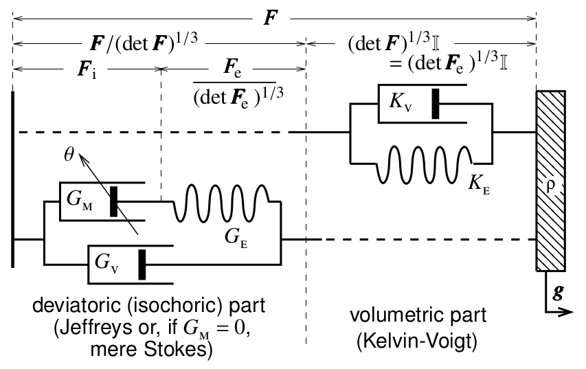
Figure 2: A schematic 0-dimensional diagramme of the mixed rheology acting differently on volumetric and the deviatoric parts: the Jeffreys rheology in the deviatoric part combines Stokes’ and Maxwell rheologies in parallel and may degenerate to mere Stokes-type fluid if $G_{\text{\sc m}}$ vanishes within melting.

Remark 3.2.

Noteworthy, the free energy (3.5a) is meant referential while the actual free energy is $\psi({\boldsymbol{F}}_{\text{\!\rm e\,}},{\boldsymbol{m}},\theta)/\!\det{\boldsymbol{F}}_{\text{\!\rm e\,}}$. The corresponding saturation magnetization $m_{\text{\sc s}}$ in zero external magnetic field as the magnitude of the minimizers of $\psi({\boldsymbol{F}}_{\text{\!\rm e\,}},\cdot,\theta)$ or, equally, of $\psi({\boldsymbol{F}}_{\text{\!\rm e\,}},\cdot,\theta)/\!\det{\boldsymbol{F}}_{\text{\!\rm e\,}}$ is given by (2.20) and is independent of ${\boldsymbol{F}}_{\text{\!\rm e\,}}$. Yet, in compressed ferromagnetic materials, the saturation magnetization as well as the Curie temperature depends on hydrostatic (or here lithostatic) pressure, cf. e.g. [15, 17, 37, 40]. This can be modelled by making $b$ in (3.5a) dependent on $\det{\boldsymbol{F}}_{\text{\!\rm e\,}}$, or even more generally replacing $b(\theta{-}\theta_{\text{\sc c}})$ in (3.5a) by $(b_{1}\theta{-}b_{2})$ with $b_{1}=b_{1}(\det{\boldsymbol{F}}_{\text{\!\rm e\,}})$ and $b_{2}=b_{2}(\det{\boldsymbol{F}}_{\text{\!\rm e\,}})$. Such generalization would not contribute to the heat capacity but would contribute to the Cauchy stress by a pressure $b_{1}^{\prime}(\det{\boldsymbol{F}}_{\text{\!\rm e\,}})|{\boldsymbol{m}}|^{2}$.

3.3 Energetics of the coupled system

To reveal the energetics behind the system (3.4) and in the particular case also behind (2.48), both considered on a fixed domain $\varOmega\subset\mathbb{R}^{3}$, needs specification of some boundary conditions on the boundary $\varGamma$ of this domain. For simplicity, let us fix it mechanically and isolate thermally by prescribing:

$${\boldsymbol{v}}=\boldsymbol{0}\,,\ \ \ \nabla{\boldsymbol{m}}{\cdot}{\boldsymbol{n}}=\boldsymbol{0}\,,\ \text{ and }\ \>\nabla\theta{\cdot}{\boldsymbol{n}}=0\ \ \ \text{ on }\ \varGamma\,,$$ (3.6)

where ${\boldsymbol{n}}$ denotes the normal to $\varGamma$. The first condition can be modified to a Navier-type condition but, minimally, the normal velocity ${\boldsymbol{v}}{\cdot}{\boldsymbol{n}}$ is to be zero to fix the domain $\varOmega$, otherwise the Eulerian formulation becomes very cumbersome. When an evolving domain is needed, some fictitious large fixed domain around the magnetoelastic material filled with “air” is used, being called a “sticky-air” approach in geophysical modelling. Let us remark that it is used also in engineering, where it is known rather as a fictitious-domain approach or as an immersed-boundary method.

The energy-dissipation balance can then be seen by testing the momentum equation (3.4b) by ${\boldsymbol{v}}$ and integrating it over $\varOmega$ while using the Green formula, the boundary conditions, and the continuity equation (LABEL:Max-Euler-thermodynam0) tested by $|{\boldsymbol{v}}|^{2}/2$ and the flow rule (3.4c) merged also with (3.4e). Further, one uses the Gilbert equation (3.4d) tested by $\mathchoice{{\buildrel\hskip 1.00006pt{{}_{{}_{\Large\boldsymbol{\circ}}}}\over{{\boldsymbol{m}}}}}{{\buildrel\hskip 1.00006pt{{}_{{}_{\Large\boldsymbol{\circ}}}}\over{{\boldsymbol{m}}}}}{{\buildrel\hskip 1.00006pt{{}_{{}_{\Large\boldsymbol{\circ}}}}\over{{\boldsymbol{m}}}}}{{\buildrel\hskip 1.00006pt{\boldsymbol{\circ}}\over{{\boldsymbol{m}}}}}$. The resulting calculations are quite demanding and we refer the reader for them to [32] and, for combination with the creep, also to [34]. The resulting balance is

$$\frac{\mathrm{d}}{\mathrm{d}t}\bigg{(}\int_{\varOmega}\!\!\!\!\!\begin{array}[t]{c}\begin{array}[t]{c}\underbrace{\frac{\varrho}{2}|{\boldsymbol{v}}|^{2}}\vspace*{.5em}\end{array}\vspace*{-1em}\\ _{\mbox{\footnotesize\rm kinetic}}\vspace*{-.5em}\\ _{\mbox{\footnotesize\rm energy}}\end{array}+\begin{array}[t]{c}\begin{array}[t]{c}\underbrace{\frac{\psi({\boldsymbol{F}}_{\text{\!\rm e\,}},{\boldsymbol{m}},0)\!\!}{\det{\boldsymbol{F}}_{\text{\!\rm e\,}}}}\vspace*{.5em}\end{array}\vspace*{-1em}\\ _{\mbox{\footnotesize\rm stored}}\vspace*{-.5em}\\ _{\mbox{\footnotesize\rm energy}}\end{array}+\begin{array}[t]{c}\begin{array}[t]{c}\underbrace{\frac{\upkappa({\boldsymbol{F}}_{\text{\!\rm e\,}})|{\nabla}{\boldsymbol{m}}|^{2}\!\!}{2\det{\boldsymbol{F}}_{\text{\!\rm e\,}}}}\vspace*{.5em}\end{array}\vspace*{-1em}\\ _{\mbox{\footnotesize\rm exchange}}\vspace*{-.5em}\\ _{\mbox{\footnotesize\rm energy}}\end{array}-\begin{array}[t]{c}\begin{array}[t]{c}\underbrace{\mu_{0}{\boldsymbol{h}}{\cdot}{\boldsymbol{m}}\!\!\!}\vspace*{.5em}\end{array}\vspace*{-1em}\\ _{\mbox{\footnotesize\rm Zeeman}}\vspace*{-.5em}\\ _{\mbox{\footnotesize\rm energy}}\end{array}\mathrm{d}{\boldsymbol{x}}$$ (3.23)

$$+\int_{\mathbb{R}^{3}}\!\!\!\!\!\!\!\!\!\!\begin{array}[t]{c}\begin{array}[t]{c}\underbrace{\frac{\mu_{0}}{2}|{\nabla}u|^{2}\!}\vspace*{.5em}\end{array}\vspace*{-1em}\\ _{\mbox{\footnotesize\rm energy of de-}}\vspace*{-.5em}\\ _{\mbox{\footnotesize\rm magnetizing field}}\end{array}\!\!\!\!\!\!\!\!\!\,\mathrm{d}{\boldsymbol{x}}\bigg{)}+\int_{\varOmega}\!\!\!\!\!\begin{array}[t]{c}\begin{array}[t]{c}\underbrace{\xi\big{(}{\boldsymbol{F}}_{\text{\!\rm e\,}},\theta;{\boldsymbol{e}}({\boldsymbol{v}}),\mathchoice{{\buildrel\hskip 1.00006pt{{}_{{}_{\Large\boldsymbol{\circ}}}}\over{{\boldsymbol{m}}}}}{{\buildrel\hskip 1.00006pt{{}_{{}_{\Large\boldsymbol{\circ}}}}\over{{\boldsymbol{m}}}}}{{\buildrel\hskip 1.00006pt{{}_{{}_{\Large\boldsymbol{\circ}}}}\over{{\boldsymbol{m}}}}}{{\buildrel\hskip 1.00006pt{\boldsymbol{\circ}}\over{{\boldsymbol{m}}}}},{\boldsymbol{L}}\big{)}\!\!}\vspace*{.5em}\end{array}\vspace*{-1em}\\ _{\mbox{\footnotesize\rm dissipation rate}}\vspace*{-.5em}\\ _{\mbox{\footnotesize\rm from \eqref{Max-Euler-thermodynam3}}}\end{array}\!\!\!\mathrm{d}{\boldsymbol{x}}=$$ (3.32)

$$=\int_{\varOmega}\!\bigg{(}\!\!\!\!\begin{array}[t]{c}\begin{array}[t]{c}\underbrace{\!\!\varrho\,{\boldsymbol{g}}{\cdot}{\boldsymbol{v}}\!\!}\vspace*{.5em}\end{array}\vspace*{-1em}\\ _{\mbox{\footnotesize\rm power of}}\vspace*{-.5em}\\ _{\mbox{\footnotesize\rm gravity field}}\end{array}\!\!\!\!\!\!-\!\!\!\!\!\begin{array}[t]{c}\begin{array}[t]{c}\underbrace{\mu_{0}\frac{\!\partial{\boldsymbol{h}}_{\text{\rm ext}}\!}{\partial t}{\cdot}{\boldsymbol{m}}}\vspace*{.5em}\end{array}\vspace*{-1em}\\ _{\mbox{\footnotesize\rm power of}}\vspace*{-.5em}\\ _{\mbox{\footnotesize\rm external field}}\end{array}\!\!\!\!$$ (3.41)

$$\begin{array}[t]{c}\begin{array}[t]{c}\underbrace{-\,\frac{\phi_{{\boldsymbol{F}}_{\text{\!\rm e\,}}}^{\prime}\!\!({\boldsymbol{F}}_{\text{\!\rm e\,}},{\boldsymbol{m}},\theta)}{\det{\boldsymbol{F}}_{\text{\!\rm e\,}}}{:}\mathchoice{{\buildrel\hskip 1.00006pt\text{\LARGE.}\over{{\boldsymbol{F}}_{\text{\!\rm e\,}}}}}{{\buildrel\hskip 1.00006pt\text{\LARGE.}\over{{\boldsymbol{F}}_{\text{\!\rm e\,}}}}}{{\buildrel\hskip 1.00006pt\text{\Large.}\over{{\boldsymbol{F}}_{\text{\!\rm e\,}}}}}{{\buildrel\hskip 1.00006pt\text{\large.}\over{{\boldsymbol{F}}_{\text{\!\rm e\,}}}}}-\frac{\phi_{\boldsymbol{m}}^{\prime}({\boldsymbol{F}}_{\text{\!\rm e\,}},{\boldsymbol{m}},\theta)\!}{\det{\boldsymbol{F}}_{\text{\!\rm e\,}}}{\cdot}\mathchoice{{\buildrel\hskip 1.00006pt\text{\LARGE.}\over{{\boldsymbol{m}}}}}{{\buildrel\hskip 1.00006pt\text{\LARGE.}\over{{\boldsymbol{m}}}}}{{\buildrel\hskip 1.00006pt\text{\Large.}\over{{\boldsymbol{m}}}}}{{\buildrel\hskip 1.00006pt\text{\large.}\over{{\boldsymbol{m}}}}}\!}\vspace*{.5em}\end{array}\vspace*{-1em}\\ _{\mbox{\footnotesize\rm adiabatic effects}}\end{array}\!\!\!\!\!\bigg{)}\,\mathrm{d}{\boldsymbol{x}}.$$ (3.45)

When we add (2.48f) tested by 1, the adiabatic and the dissipative heat sources cancel with those in (3.45). Thus we obtain the total energy balance

$$\frac{\mathrm{d}}{\mathrm{d}t}\bigg{(}\int_{\varOmega}\!\!\!\!\!\begin{array}[t]{c}\begin{array}[t]{c}\underbrace{\frac{\varrho}{2}|{\boldsymbol{v}}|^{2}}\vspace*{.5em}\end{array}\vspace*{-1em}\\ _{\mbox{\footnotesize\rm kinetic}}\vspace*{-.5em}\\ _{\mbox{\footnotesize\rm energy}}\end{array}+\begin{array}[t]{c}\begin{array}[t]{c}\underbrace{\frac{\psi({\boldsymbol{F}}_{\text{\!\rm e\,}},{\boldsymbol{m}},0)}{\det{\boldsymbol{F}}_{\text{\!\rm e\,}}}+\omega({\boldsymbol{F}}_{\text{\!\rm e\,}},{\boldsymbol{m}},\theta)}\vspace*{.5em}\end{array}\vspace*{-1em}\\ _{\mbox{\footnotesize\rm internal energy}}\end{array}\!\!\!\!$$ (3.53)

$$+\!\!\!\!\!\!\begin{array}[t]{c}\begin{array}[t]{c}\underbrace{\frac{\upkappa({\boldsymbol{F}})|{\nabla}{\boldsymbol{m}}|^{2}}{2\det{\boldsymbol{F}}}}\vspace*{.5em}\end{array}\vspace*{-1em}\\ _{\mbox{\footnotesize\rm exchange}}\vspace*{-.5em}\\ _{\mbox{\footnotesize\rm energy}}\end{array}-\begin{array}[t]{c}\begin{array}[t]{c}\underbrace{\mu_{0}{\boldsymbol{h}}{\cdot}{\boldsymbol{m}}\!\!\!}\vspace*{.5em}\end{array}\vspace*{-1em}\\ _{\mbox{\footnotesize\rm Zeeman}}\vspace*{-.5em}\\ _{\mbox{\footnotesize\rm energy}}\end{array}\!\!\!\!\,\mathrm{d}{\boldsymbol{x}}+\int_{\mathbb{R}^{3}}\begin{array}[t]{c}\begin{array}[t]{c}\underbrace{\frac{\mu_{0}}{2}|{\nabla}u|^{2}\!\!}\vspace*{.5em}\end{array}\vspace*{-1em}\\ _{\mbox{\footnotesize\rm energy of de-}}\vspace*{-.5em}\\ _{\mbox{\footnotesize\rm magnetizing field}}\end{array}\mathrm{d}{\boldsymbol{x}}\bigg{)}$$ (3.66)

$$\hskip 60.00009pt=\int_{\varOmega}\!\!\!\!\!\begin{array}[t]{c}\begin{array}[t]{c}\underbrace{\varrho{\boldsymbol{g}}{\cdot}{\boldsymbol{v}}}\vspace*{.5em}\end{array}\vspace*{-1em}\\ _{\mbox{\footnotesize\rm power of}}\vspace*{-.5em}\\ _{\mbox{\footnotesize\rm gravity}}\vspace*{-.5em}\\ _{\mbox{\footnotesize\rm field}}\end{array}\!\!\!\!\!\!\!\!-\!\!\!\!\!\!\begin{array}[t]{c}\begin{array}[t]{c}\underbrace{\mu_{0}\frac{\!\partial{\boldsymbol{h}}_{\text{\rm ext}}\!}{\partial t}{\cdot}{\boldsymbol{m}}}\vspace*{.5em}\end{array}\vspace*{-1em}\\ _{\mbox{\footnotesize\rm power of}}\vspace*{-.5em}\\ _{\mbox{\footnotesize\rm external field}}\end{array}\!\!\!\!\mathrm{d}{\boldsymbol{x}}\,,$$ (3.76)

where $\omega({\boldsymbol{F}}_{\text{\!\rm e\,}},{\boldsymbol{m}},\theta)$ is from (2.45). The skew-symmetric stress $\SS$ and hyperstress $\mathscr{S}$ in (2.48b) used also in (3.4b) were devised just to facilitate this desired energetics, see [32, Sect.2.4].

3.4 Remarks to analysis of a multipolar variant

The rigorous mathematical analysis of the above models seems problematic and there is a certain agreement that some higher-gradient theories must be involved in them to pursue this analytical goal. Our approach follows the theory by [11], as already considered in the general nonlinear context of so-called multipolar fluids by J. Nečas and his group, cf. [25, 26, 27], as originally inspired by [38] and [24]. Also, the gradient of the inelastic distortion rate ${\boldsymbol{L}}$ is to be involved.

The dissipation potential $\zeta$ extends by the higher-order terms $\nu_{1}|\nabla^{2}{\boldsymbol{v}}|^{p}/p$ with $p>3$ and $\nu_{2}|\nabla{\boldsymbol{L}}|^{2}/2$. This brings an additional hyper-stress contribution to the Cauchy stress, namely ${\rm div}(\nu_{1}|\nabla^{2}{\boldsymbol{v}}|^{p-2}\nabla^{2}{\boldsymbol{v}})$, and an contribution ${\rm div}(\nu_{2}\nabla{\boldsymbol{L}})$ to the Mandel stress on the right-hand side of (3.4e). The dissipation rate $\xi$ in (3.4g) expands by $\nu_{1}|\nabla^{2}{\boldsymbol{v}}|^{p}+\nu_{2}|\nabla{\boldsymbol{L}}|^{2}$, as well as the boundary conditions should be extended appropriately, cf. [31, 32, 34] for quite nontrivial analytical details.

4 Paleomagnetism in crustal rocks

The above devised model (3.4) with (3.5) can directly be applied to thermoremanent paleomagnetism in crustal rocks. Although the seven-equation system (3.4) may seem too complicated, it should be pointed out that it is a minimal scenario if one wants to cover the involved thermomechanical and thermomagnetical processes, as was indicated in Figure 1.

The modeling is based on a suitable temperature dependence of the Maxwellian creep modulus $G_{\text{\sc m}}$ in (3.4e), the saturation magnetization $m_{\text{\sc s}}$ in (2.20), the coercive force $h_{\rm c}$ in (3.4d). The mentioned temperature dependence of $m_{\text{\sc s}}$ can be performed by an appropriate choice of the Curie temperature $\theta_{\text{\sc c}}$ in (2.19). The mentioned temperature dependence of $G_{\text{\sc m}}$ allows for modelling of the transition between a very fluidic phase (with low $G_{\text{\sc m}}$ of the order $10^{4\pm 3}$Pa s) to rather solid rocks (with high $G_{\text{\sc m}}$ of the order $10^{22\pm 2}$Pa s). The mentioned temperature dependence of $h_{\rm c}$ allows for “freezing” the magnetization ${\boldsymbol{m}}$ in rocks when they become sufficiently cold, well below the Curie temperature. All three mentioned transitions should be properly ordered with respect to temperature, cf. Figure 3.

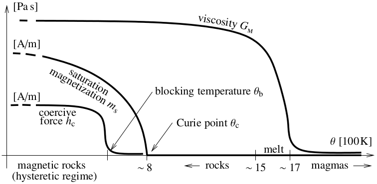
Figure 3: Some temperature-dependent magnetic properties behind ferri-to-antiferromagnetic phase transition in solid rocks and mechanical properties behind melting of rocks towards magma.

The external field ${\boldsymbol{h}}_{\rm ext}$ then plays the role as the geomagnetic field generated in outer core by magnetodynamical mechanism.

It is important that rocks even with magnetic minerals undergoing the antiferro-to-ferri magnetic transition rather than metals undergoing the para-to-ferro magnetic transition are electrically not conductive. This is why we could consider only magneto-static approximation of the full Maxwell electromagnetic system in (2.24) and neglected any eddy currents.

The rate-dependent $\alpha$- and $\gamma$-terms in (3.4g) are actually quite irrelevant within slow thermoremanent magnetization and subsequent mechanical evolution within million-year time scale in crustal rocks. Yet, they can be relevant within fast processes in flash magnetization due to strong magnetic fields as occurs in lightening. This is the mechanism behind the isothermal remanent magnetization in cold crustal rocks.

Besides these two, there is also a viscous remanent magnetization which may occur when rocks are exposed in a sufficiently long time by modern-day magnetic fields which are stronger than geomagnetic field but anyhow not so strong to lead to an immediate (re)magnetization. This would need a modification of the linear term $\alpha\mathchoice{{\buildrel\hskip 1.00006pt{{}_{{}_{\Large\boldsymbol{\circ}}}}\over{{\boldsymbol{m}}}}}{{\buildrel\hskip 1.00006pt{{}_{{}_{\Large\boldsymbol{\circ}}}}\over{{\boldsymbol{m}}}}}{{\buildrel\hskip 1.00006pt{{}_{{}_{\Large\boldsymbol{\circ}}}}\over{{\boldsymbol{m}}}}}{{\buildrel\hskip 1.00006pt{\boldsymbol{\circ}}\over{{\boldsymbol{m}}}}}$ in (3.4d) to a nonlinear, piecewise linear term distinguishing slow and fast magnetization or, in other words, a nonquadratic modification of the quadratic term $\alpha|{\boldsymbol{r}}|^{2}/2$ in the dissipation potential (3.5a).

Remark 4.1 (Heterogeneous model).

Rocks in wider spacial areas are typically substantially heterogeneous, as also depicted in Fig. 1. This can be included in the model, beside ${\boldsymbol{X}}$-dependence of the initial conditions, also by allowing for an ${\boldsymbol{X}}$-dependence of the data $\psi$, ${\mathbb{D}}$, and $h_{\text{\rm c}}$. In Eulerian formulation, ${\boldsymbol{X}}$ serves as a placeholder for $\boldsymbol{\xi}({\boldsymbol{x}})$ and then the transport equation (2.2) for $\boldsymbol{\xi}$ is to be added into the system, cf. [34] for a non-magnetic merely thermomechanical variant of this system.

Remark 4.2 (A linearized convective model).

Geophysical modelling at large displacements but small elastic strain uses, instead of the deformation gradient ${\boldsymbol{F}}$ and the multiplicative decomposition, rather a small strain ${\boldsymbol{e}}({\boldsymbol{u}})$ with the displacement ${\boldsymbol{u}}={\boldsymbol{y}}\,{-}\,$identity and its Green-Naghdi’s additive decomposition to the elastic and the inelastic strains expressed in rates using the Zaremba-Jaumann derivative of these strains. Such linearization of the model (3.4) was devised by [33].

Acknowledgment. Support from the CSF grant no. 23-06220S and the institutional support RVO: 61388998 (ČR) is gratefully acknowledged.

References

- [1] W. Baltensperger and J. S. Helman. Dry friction in micromagnetics. IEEE Trans. Magnet., 27:4772–4774, 1991.
- [2] B. Benešová, J. Forster, C. Liu, and A. Schlömerkemper. Existence of weak solutions to an evolutionary model for magnetoelasticity. SIAM J. Math. Anal., 50:1200–1236, 2018.
- [3] G. Bertotti. Hysteresis in Magnetism. Academic Press, San Diego, 1998.
- [4] W. F. Brown Jr. Magnetoelastic Interactions. Springer, Berlin, 1966.
- [5] R. F. Butler. Paleomagnetism: Magnetic Domains to Geologic Terranes. Blackwell Sci. Inc., 1992.
- [6] W. H. Campbell. Introduction to Geomagnetic Fields. Cambridge Univ. Press, Cambridge, 2 edition, 2003.
- [7] A. Cox and R. R. Doell. Review of paleomagnetism. Geol. Soc. Amer. Bull., 71:645–768, 1960.
- [8] A. DeSimone and P. Podio Guidugli. Inertial and self interactions in structured continua: Liquid crystals and magnetostrictive solids. Meccanica, 300:629–640, 1995.
- [9] A. DeSimone and P. Podio Guidugli. On the continuum theory of deformable ferromagnetic solids. Arch. Rat. Mech. Anal., 136:201–233, 1996.
- [10] D. J. Dunlop and Ö. Özdemir. Rock Magnetism. Cambridge Univ. Press, Cambridge, 1997.
- [11] E. Fried and M. E. Gurtin. Tractions, balances, and boundary conditions for nonsimple materials with application to liquid flow at small-lenght scales. Arch. Ration. Mech. Anal., 182:513–554, 2006.
- [12] H. Garcke, P. Knopf, S. Mitra, and A. Schlömerkemper. Strong well-posedness, stability and optimal control theory for a mathematical model for magneto-viscoelastic fluids. Calc. Var., 61:Art.no.179, 2022.
- [13] T.L. Gilbert. A Lagrangian formulation of the gyromagnetic equation of the magnetization field. Phys. Rev., 100:1243, 1955.
- [14] G. Grün and P. Weiss. On the field-induced transport of magnetic nanoparticles in incompressible flow: Existence of global solutions. J. Math. Fluid Mech., 23:Art.no.10, 2021.
- [15] D. Gugan. The change of spontaneous magnetization with hydrostatic pressure. Proc. Phys. Soc., 72:1013–1026, 1958.
- [16] M. Kalousek, J. Kortum, and A. Schlömerkemper. Mathematical analysis of weak and strong solutions to an evolutionary model for magnetoviscoelasticity. Disc. Cont. Dynam. Systems - S, 14:17–39, 2021.
- [17] J.S. Kouvak and R.H. Wilson. Magnetization of Iron-Nickel alloys under hydrostatic pressure. J. Appl. Phys., 32:435–441, 1961.
- [18] E. Kröner. Allgemeine Kontinuumstheorie der Versetzungen und Eigenspannungen. Arch. Ration. Mech. Anal., 4:273–334, 1960.
- [19] L. D. Landau. On the theory of phase transitions. Zh. Eksp. Teor. Fiz., 7:19–32, 1937.
- [20] L. D. Landau and E. M. Lifshitz. On the theory of dispersion of magnetic permeability in ferromagnetic bodies. Phys. Z. Sowjet., 8 (153):153–169, 1935.
- [21] R. Lanza and A. Meloni. The Earth’s Magnetism. Springer, Berlin, 2006.
- [22] E. Lee and D. Liu. Finite-strain elastic-plastic theory with application to plain-wave analysis. J. Applied Phys., 38:19–27, 1967.
- [23] G. A. Maugin. A continuum theory of deformable ferrimagnetic bodies. I. Field equations. J. Math. Phys., 117:1727–1738, 1976.
- [24] R.D. Mindlin. Micro-structure in linear elasticity. Archive Ration. Mech. Anal., 16:51–78, 1964.
- [25] J. Nečas. Theory of multipolar fluids. In L. Jentsch and F. Tröltzsch, editors, Problems and Methods in Mathematical Physics, pages 111–119, Wiesbaden, 1994. Vieweg+Teubner.
- [26] J. Nečas, A. Novotný, and M. Šilhavý. Global solution to the ideal compressible heat conductive multipolar fluid. Comment. Math. Univ. Carolinae, 30:551–564, 1989.
- [27] J. Nečas and M. Ržička. Global solution to the incompressible viscous-multipolar material problem. J. Elasticity, 29:175–202, 1992.
- [28] P. Podio-Guidugli. On dissipation mechanisms in micromagnetics. Eur. Phys J. B., 19:417–424, 2001.
- [29] P. Podio-Guidugli, T. Roubíček, and G. Tomassetti. A thermodynamically-consistent theory of the ferro/paramagnetic transition. Archive Rat. Mech. Anal., 198:1057–1094, 2010.
- [30] T Roubíček. Microstructure in ferromagnetics and its steady-state and evolution model. In M. Robnik and A.Ruffing, editors, Comm. Bexbach Colloquium on Science, Vol.II, pages 39–52, Aachen, 2003. Shaker Verlag.
- [31] T. Roubíček. Quasistatic hypoplasticity at large strains Eulerian. J. Nonlin. Sci., 32:Art.no.45., 2022.
- [32] T. Roubíček. Landau theory for ferro-paramagnetic phase transition in finitely-strained viscoelastic magnets. Math. Models Methods Appl. Sci. (submitted), 2023. Preprint arXiv no.2302.02850.
- [33] T. Roubíček. A thermodynamical model for paleomagnetism in Earth’s crust. Math. Mech. Solids, 28:1063–1090, 2023.
- [34] T. Roubíček and G. Tomassetti. Inhomogeneous finitely-strained thermoplasticity with hardening by an Eulerian approach. Disc. Cont. Dynam. System - S,, printed on line, 2023.
- [35] T. Roubíček, G. Tomassetti, and C. Zanini. The Gilbert equation with dry-friction-type damping. J. Math. Anal. Appl., 355:453–468, 2009.
- [36] F. D. Stacey and S. K. Banerjee. The Physical Principles of Rock Magnetism. Elsevier, Amsterdam, 1974.
- [37] F.D. Stacey. The behavior of ferromagnetics under strong compression. Canadian J. Phys., 34:304–311, 1956.
- [38] R. A. Toupin. Elastic materials with couple stresses. Arch. Ration. Mech. Anal., 11:385–414, 1962.
- [39] R. A. Toupin. Theories of elasticity with couple stresses. Arch. Ration. Mech. Anal., 17:85–112, 1964.
- [40] J. Valenta at al. Pressure-induced large increase of Curie temperature of the van der Waals ferromagnet VI3. Phys. Rev. B, 103:Art.no.054424, 2021.
- [41] A. Visintin. Modified Landau-Lifshitz equation for ferromagnetism. Phys. B, 233:365–369, 1997.
- [42] W. Zhao. Local well-posedness and blow-up criteria of magneto-viscoelastic flow. Disc. Cont. Dynam. Syst., 38:4637–4655, 2018.