Randomized semi-quantum matrix processing

Abstract

Quantum computers have the potential to speed-up important matrix-arithmetic tasks. A prominent framework for that is the quantum singular-value transformation (QSVT) formalism, which uses Chebyshev approximations and coherent access to the input matrix via a unitary block encoding to design a target matrix function. Nonetheless, physical implementations for useful end-user applications require large-scale fault-tolerant quantum computers. Here, we present a hybrid quantum-classical framework for Monte-Carlo simulation of generic matrix functions more amenable to early fault-tolerant quantum hardware. Serving from the ideas of QSVT, we randomize over the Chebyshev polynomials while keeping the matrix oracle quantum. The method is assisted by a variant of the Hadamard test that removes the need for post-selection. As a result, it features a statistical overhead similar to the fully quantum case of standard QSVT and do not incur any circuit depth degradation. On the contrary, the average circuit depth is shown to get smaller, yielding equivalent reductions of noise sensitivity, as we explicitly show for depolarizing noise and coherent errors. We apply our technique to four specific use cases: partition-function estimation via quantum Markov-chain Monte Carlo and via imaginary-time evolution; end-to-end linear system solvers; and ground-state energy estimation. For these cases, we prove advantages on average depths, including quadratic speed-ups on costly parameters and even the removal of the approximation-error dependence. All in all, our framework provides a pathway towards early fault-tolerant quantum linear algebra applications.

I Introduction

Faster algorithms for linear algebra are a major promise of quantum computation, holding the potential for precious runtime speed-ups over classical methods. A modern, unified framework for such algorithms is given by the quantum signal processing (QSP) LowChuang2017 ; LowChuangQuantum2019 and, more generally, quantum singular-value transformation (QSVT) Gilyen2019 formalisms. These are powerful techniques to manipulate a matrix, coherently given by a quantum oracle, via polynomial transformations on its eigenvalues and singular values, respectively. The class of matrix arithmetic attained is remarkably broad, encompassing primitives as diverse as Hamiltonian simulation, matrix inversion, ground-state energy estimation, Gibbs-state sampling, among others ChuangGrandUnification . Moreover, the framework often offers the state-of-the-art in asymptotic query complexities (i.e. number of oracle calls), in some cases matching known complexity lower bounds. Nevertheless, the experimental requirements for full implementations are prohibitive for current devices, and it is not clear if the framework will be useful in practice before large-scale fault-tolerant quantum computers appear.

This has triggered a quest for early fault-tolerant algorithms for matrix processing that allow one to trade performance for nearer-term feasibility in a controlled way, i.e. with provable runtime guarantees silva_fragmented_2022 ; silva2022fourierbased ; lin_heisenberg-limited_2022 ; wang_quantum_2022 ; campbell_random_2019 ; wan_randomized_2022 ; wang2023qubitefficient ; Campbell_2021 ; Dong_2022 ; wang2023faster . Particularly promising are randomized hybrid quantum-classical schemes to statistically simulate a matrix function via quantum implementations of more elementary ones lin_heisenberg-limited_2022 ; wang_quantum_2022 ; campbell_random_2019 ; wan_randomized_2022 ; wang2023qubitefficient ; Campbell_2021 . For instance, this has been applied to the Heaviside step function $\theta(H)$ of a Hamiltonian $H$, which allows for eigenvalue thresholding, a practical technique for Heisenberg-limited spectral analysis lin_heisenberg-limited_2022 . Two input access models have been considered there: quantum oracles as a controlled unitary evolution of $H$ lin_heisenberg-limited_2022 ; wang_quantum_2022 ; Dong_2022 and classical ones given by a decomposition of $H$ as a linear combination of Pauli operators campbell_random_2019 ; wan_randomized_2022 ; wang2023qubitefficient ; Campbell_2021 . In the former, one Monte-Carlo simulates the Fourier series of $\theta(H)$ by randomly sampling its harmonics. In the latter – in an additional level of randomization – one also probabilistically samples the Pauli terms from the linear combination.

Curiously, however, randomized quantum algorithms for matrix processing have been little explored beyond the specific case of the Heaviside function. Ref. wang2023qubitefficient put forward a randomized, qubit-efficient technique for Fourier-based QSP silva2022fourierbased ; Dong_2022 for generic functions. However, the additional level of randomization can detrimentally affect the circuit depth per run, as compared to the case with coherent oracles. On the other hand, in the quantum-oracle setting, the randomized algorithms above have focused mainly on controlled unitary evolution as the input access model. This is convenient in specific cases where $H$ can be analogically implemented. However, it leaves aside the powerful class of block-encoding oracles, i.e. unitary matrices with the input matrix as one of its blocks LowChuangQuantum2019 . Besides having a broader scope of applicability (including non-Hermitean matrices), such oracle types are also a more natural choice for digital setups. Moreover, randomized quantum algorithms have so far not addressed Chebyshev polynomials, the quintessential basis functions for approximation theory trefethen_approx , which often attain better accuracy than Fourier series boyd_spectral_methods . Chebyshev polynomials, together with block-encoding oracles, provide the most sophisticated and general arena for quantum matrix arithmetic LowChuang2017 ; LowChuangQuantum2019 ; Gilyen2019 ; ChuangGrandUnification .

Here, we fill in this gap. We derive a semi-quantum algorithm for Monte-Carlo simulations of QSVT with provably better circuit complexities than fully-quantum schemes as well as notable advantages in terms of experimental feasibility. Our results are summarized next.

II Summary of our contributions

Our method estimates state amplitudes and expectation values involving a generic matrix function $f(A)$ leveraging three main ingredients: $i$) it samples each component of a Chebyshev series for $f$ with a probability proportional to its coefficient in the series; $ii$) it assumes coherent access to $A$ via a block-encoding oracle; and $iii$) $f(A)$ is automatically extracted from its block-encoding without post-selection, using a Hadamard test. The combination of $i$) and $ii$) leaves untouched the maximal query complexity $k$ per run native from the Chebyshev expansion. In addition, the statistical overhead we pay for end-user estimations scales only with the $l_{1}$-norm of the Chebyshev coefficients. For the use cases we consider, this turns out to be similar (at worst up to logarithmic factors) to the operator norm of $f(A)$, which would govern the statistical overhead if we used fully-quantum (i.e. standard) QSVT. That is, our scheme does not incur any significant degradation with respect to the fully-quantum case either in runtime or circuit depth. On the contrary, the average query complexity can be significantly smaller than $k$. We prove interesting speed-ups of the former over the latter for practical use cases.

These speed-ups translate directly into equivalent reductions in noise sensitivity: For simple models such as depolarization or coherent errors in the quantum oracle, we show that the estimation inaccuracy caused by noise scales with the average query depth. In comparison, it scales with the maximal depth in standard QSVT implementations. Importantly, we implement each sampled Chebyshev polynomial with a simple sequence of queries to the oracle using qubitization; no QSP pulses are required throughout. Finally, $iii$) circumvents the need for expensive repeat until success or quantum amplitude amplification. That is, no statistical run is wasted, and no overhead in circuit depth is incurred. The only price paid is the need for the control qubit in the Hadamard test, but fully quantum implementations would require yet another ancilla controlling everything else (due to the QSP pulses). All this renders our hybrid approach more experimentally friendly than coherent QSVT.

As use cases, we benchmark our framework on four end-user applications: partition-function estimation of classical Hamiltonians via quantum Markov-chain Monte Carlo (MCMC); partition-function estimation of quantum Hamiltonians via quantum imaginary-time evolution (QITE); linear system solvers (LSSs); and ground-state energy estimation (GSEE). The maximal and expected query depths per run as well as the total expected runtime (taking into account sample complexity) are displayed in Table 1, in Sec. IV.4. In all cases, we systematically obtain the following advantages (both per run and in total) of expected versus maximal query complexities.

For MCMC, we prove a quadratic speed-up on a factor $\mathcal{O}(\log(Z_{\beta}\,e^{\beta}/\epsilon_{\text{r}}))$, where $Z_{\beta}$ is the partition function to estimate, at inverse temperature $\beta$, and $\epsilon_{\text{r}}$ is the tolerated relative error. For QITE, we remove a factor $\mathcal{O}(\log(D\,e^{\beta}/Z_{\beta}\,\epsilon_{\text{r}}))$ from the scaling, where $D$ is the system dimension. For LSSs we consider two sub-cases: estimation of an entry of the (normalized) solution vector and of the expectation value of an observable $O$ on it. We prove quadratic speed-ups on factors $\mathcal{O}\big{(}\log(\kappa/\epsilon)\big{)}$ and $\mathcal{O}\big{(}\log(\kappa^{2}\,\|O\|/\epsilon)\big{)}$ for the first and second sub-cases, respectively, where $\|O\|$ is the operator norm of $O$, $\kappa$ is the condition number of the matrix, and $\epsilon$ the tolerated additive error. Remarkably, this places our query depth at an intermediate position between that of the best known Chebyshev-based method Childs_2017 and the optimal one in general costa2021optimal . In turn, compared to the results obtained in wang2023qubitefficient via full randomization, our scaling is one power of $\kappa$ superior. Finally, for GSEE, we prove a speed-up on a factor that depends on the overlap $\eta$ between the probe state and the ground state: the average query depth is $\mathcal{O}\big{(}\frac{1}{\xi}\sqrt{\log(1/\eta)}/\log(1/\xi)\big{)}$, whereas the maximal query depth is $\mathcal{O}\big{(}\frac{1}{\xi}\log(1/\eta)\big{)}$, with $\xi$ the additive error in the energy estimate.

Our method reduces the experimental requirements for early fault-tolerant quantum linear algebra applications.

III Preliminaries

We consider the basic setup of Quantum Singular Value Transformation (QSVT) Gilyen2019 ; ChuangGrandUnification . This is a powerful technique for synthesizing polynomial functions of a linear operator embedded in a block of a unitary matrix, via polynomial transformations on its singular values. Combined with approximation theory Vishnoi2013 , this leads to state-of-the-art query complexities and an elegant unifying structure for a variety of quantum algorithms of interest. For simplicity of the presentation, in the main text we focus explicitly on the case of Hermitian matrices. There, QSVT reduces to the simpler setup of Quantum Signal Processing (QSP) LowChuang2017 ; LowChuangQuantum2019 , describing eigenvalue transformations. The extension of our algorithms to QSVT for generic matrices is straightforward and is left for App. G. Throughout the paper, we adopt the short-hand notation $[l]:=\{0,\ldots,l-1\}$ for any $l\in\mathbb{N}$.

The basic input taken by QSP is a block-encoding $U_{A}$ of the Hermitian operator $A$ of interest (the signal). A block-encoding is a unitary acting on $\mathcal{H}_{sa}:=\mathcal{H}_{s}\otimes\mathcal{H}_{a}$, where $\mathcal{H}_{s}$ is the system Hilbert space where $A$ acts and $\mathcal{H}_{a}$ is an ancillary Hilbert space (with dimensions $D$ and $D_{a}$, respectively), satisfying

$$\big{(}\bra{0}_{a}\otimes\mathds{1}_{s}\big{)}\,U_{A}\,\big{(}\ket{0}_{a}\otimes\mathds{1}_{s}\big{)}=A$$ (1)

for some suitable state $\ket{0}_{a}\in\mathcal{H}_{a}$ (here $\mathds{1}_{s}$ is the identity operator in $\mathcal{H}_{s}$). Designing such an oracle for arbitrary $A$ is a non-trivial task camps2023explicit , but efficient block-encoding schemes are known in cases where some special structure is present, e.g., when $A$ is sparse or expressible as a linear combination of unitaries LowChuangQuantum2019 ; Gilyen2019 ; sunderhauf2023blockencoding . In particular, we will need the following particular form of $U_{A}$ that makes it amenable for dealing with Chebyshev polynomials.

Definition 1 (Qubitized block-encoding oracle).

Let $A$ be a Hermitian matrix on $\mathcal{H}_{s}$ with spectral norm $\norm{A}\leq 1$, eigenvalues $\{\lambda_{\gamma}\}_{\gamma\in[D]}$, and eigenstates $\{\ket{\lambda}_{s}\}$. A unitary $U_{A}$ acting on $\mathcal{H}_{sa}$ is called a (exact) qubitized block-encoding of $A$ if it has the form

$$U_{A}=\bigoplus_{\gamma\in[D]}e^{-i\,\vartheta_{\gamma}\,Y_{\gamma}}\,,$$ (2)

where $\vartheta_{\gamma}:=\arccos(\lambda_{\gamma})$ and $Y_{\gamma}$ is the second Pauli matrix acting on the two-dimensional subspace spanned by $\big{\{}\ket{0}_{a}\otimes\ket{\lambda_{\gamma}}_{s},\ket{\perp_{\lambda_{\gamma}}}_{sa}\big{\}}$ with ${}_{sa}\!\bra{\perp_{\lambda_{\gamma}}}\big{(}\ket{0}_{a}\otimes\ket{\lambda_{\gamma}}_{s}\big{)}=0$.

A qubitized oracle of the form (2) can be constructed from any other block-encoding $U^{\prime}_{A}$ of $A$ using at most one query to $U^{\prime}_{A}$ and ${U^{\prime}_{A}}^{-1}$, at most one additional ancillary qubit, and $\mathcal{O}(\log(D_{a}))$ quantum gates LowChuangQuantum2019 .

Standard QSP takes as input the qubitized oracle $U_{A}$ and transforms it into (a block-encoding of) a polynomial function $\tilde{f}(A)$. With the help of function approximation theory trefethen_approx , this allows the approximate implementation of generic non-polynomial functions $f(A)$. The algorithm complexity is measured by the number of queries to $U_{A}$, which allows for rigorous quantitative statements agnostic to details of $A$ or to hardware-specific circuit compilations. For our purposes, only a simple QSP result will be needed, namely the observation LowChuangQuantum2019 that repeated applications of $U_{A}$ give rise to Chebyshev polynomials of $A$ (see App. A for a proof).

Lemma 2 (Block encoding of Chebyshev polynomials).

Let $U_{A}$ be a qubitized block-encoding of $A$. Then

$$\big{(}\bra{0}_{a}\otimes\mathds{1}_{s}\big{)}\,U_{A}^{j}\,\big{(}\ket{0}_{a}\otimes\mathds{1}_{s}\big{)}=\mathcal{T}_{j}(A)\,,$$ (3)

for $j\in\mathbb{N}$, where $\mathcal{T}_{j}(\cdot)$ is the $j$-th order Chebyshev polynomial of the first kind.

We are interested in a truncated Chebyshev series

$$\tilde{f}(x)=\sum^{k}_{j=0}a_{j}\mathcal{T}_{j}(x)$$ (4)

providing a $\nu$-approximation to the target real-valued function $f:[-1,1]\rightarrow\mathbb{R}$, that is, $\max_{x\in[-1,1]}\absolutevalue{f(x)-\tilde{f}(x)}\leq\nu$. The Chebyshev polynomials $\mathcal{T}_{j}$ form a key basis for function approximation, often leading to near-optimal approximation errors trefethen_approx . In particular, unless the target function is periodic and smooth, they tend to outperform Fourier approximations boyd_spectral_methods . The case of complex-valued functions can be treated similarly by splitting it into its real and imaginary parts. The truncation order $k$ is controlled by the desired accuracy $\nu$ in a problem-specific way (see Sec. IV.4 for explicit examples). We denote by $\boldsymbol{a}:=\big{\{}a_{0},\ldots,a_{k}\big{\}}$ the vector of Chebyshev coefficients of $\tilde{f}$ and by $\norm{\boldsymbol{a}}_{1}:=\sum_{j=0}^{k}|a_{j}|$ its $\ell_{1}$-norm.

IV Results

We are now in a position to state our main results. First, we set up explicitly the two problems of interest and then proceed to describe our randomized semi-quantum algorithm to solve each one of them, proving correctness, runtime, and performing an error-robustness analysis. We conclude by applying our general framework to a number of exemplary use cases of interest.

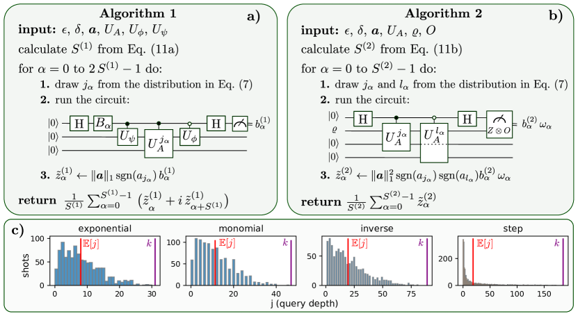
Figure 1: Alg. 1 in panel a) solves Problem 1, whereas Alg. 2 in panel b) solves Problem 2. a-b) The algorithms receive as inputs: $i)$ a qubitized block-encoding $U_{A}$ of $A$; $ii)$ the vector $\boldsymbol{a}$ of Chebyshev coefficients defining the polynomial approximation $\tilde{f}$ to the target function $f$; $iii)$ state preparation unitaries $U_{\phi}$ and $U_{\psi}$ (for Alg. 1), or the state $\varrho$ and the observable $O$ (for Alg. 2); $iv)$ the tolerated error $\epsilon$ and failure probability $\delta$ for the statistical estimation. The algorithm repeats a number $\frac{2}{P}S^{(P)}$ of times two basic sampling steps. The first step is to classically sample a Chebyshev polynomial degree $j_{\alpha}$ with probability $p(j_{\alpha})=|a_{j_{\alpha}}|/\norm{\boldsymbol{a}}_{1}$. The second step – the only quantum subroutine – is a Hadamard test (including a measurement of $O$, for Alg. 2) containing $j_{\alpha}$ successive queries to the controlled version of $U_{A}$ (plus another sequence of $l_{\alpha}$ queries but with the control negated and a different oracle-ancilla register for Alg. 2). Finally, the average over all the measurement outcomes gives the statistical estimate of the quantity of interest $z^{(P)}$, for $P=1$ or 2. Interestingly, the Hadamard test automatically extracts the correct block of $U_{A}$, which relaxes the need for post-selection on the oracle ancillae. Therefore, every experimental run contributes to the statistics (i.e., no measurement shot is wasted). c) Histograms of number of times (shots) a Chebyshev polynomial degree $j$ is drawn out of $1000$ samples, for the four use cases described in Sec. IV.4. The vertical lines show the maximal Chebyshev degree $k$ (purple) and the average degree $\mathbb{E}[j]$ (red). Importantly, for this figure, we do not estimate $k$ analytically using approximation theory. The values of $k$ plotted are numerically obtained as the minimum degree of $\tilde{f}$ such that the target error $\nu$ is attained. The parameters used are: $\nu=10^{-2}$ (all examples), $\beta=100$ (exponential function), $t=200$ (monomial), $\kappa=8$ (inverse function), $\mu=20$ (step function). In all cases, we observe a significant reduction in query complexity. This translates in practice into shallower circuits and hence less accumulated noise (see Sec. IV.3).

IV.1 Problem statement

We consider the following two concrete problems (throughout the paper we will use superscripts ⁽¹⁾ or ⁽²⁾ on quantities referring to Problems 1 or 2, respectively):

Problem 1 (Transformed vector amplitudes).

Given access to state preparation unitaries $U_{\phi}$ and $U_{\psi}$ such that $U_{\psi}\ket{0}=\ket{\psi}$, $U_{\phi}\ket{0}=\ket{\phi}$, a Hermitean matrix $A$, and a real-valued function $f$, obtain an estimate of

$$z^{(1)}=\matrixelement{\phi}{f(A)}{\psi}$$ (5)

to additive precision $\epsilon$ with failure probability at most $\delta$.

This class of problems is relevant for estimating the overlap between a linearly transformed state and another state of interest. This is the case, e.g., in linear system solving, where one is interested in the $i$-th computational basis component of a quantum state of the form $A^{-1}\ket{\boldsymbol{b}}$ encoding the solution to the linear system (see Sec. IV.4.2 for details). The unitary $U_{\phi}$ preparing the computational-basis state $\ket{i}$, in that case, is remarkably simple, given by a sequence of bit flips.

Problem 2 (Transformed observable expectation values).

Given access to a state preparation $\varrho$, a Hermitian matrix $A$, an observable $O$, and a real-valued function $f$, obtain an estimate of

$$z^{(2)}=\Tr[O\,f(A)\,\varrho\,f(A)^{\dagger}]$$ (6)

to additive precision $\epsilon$ with failure probability at most $\delta$.

This is of relevance, e.g., when $A=H$ is a Hamiltonian, to estimate the partition function corresponding to $H$, as discussed below in Sec. IV.4.1.

We present randomized hybrid classical-quantum algorithms for these problems using Chebyshev-polynomial approximations of $f$ and coherent access to a block-encoding of $A$. Similar problems have been addressed in wang2023qubitefficient but using Fourier approximations and randomizing also over a classical description of $A$ in the Pauli basis.

IV.2 Randomized semi-quantum matrix processing

Our framework is based on the Chebyshev approximation $\tilde{f}$ of the function $f$ and a modified Hadamard test involving the qubitized block-encoding oracle $U_{A}$. The idea is to statistically simulate the coherent QSP algorithm using a hybrid classical/quantum procedure based on randomly choosing $j\in[k+1]$ according to its importance for Eq. (4) and then running a Hadamard test involving the block encoding $U_{A}^{j}$ of $\mathcal{T}_{j}(A)$. Pseudo-codes for the algorithms are presented in Fig. 1. a) and 1. b) for Problems 1 and 2, respectively. In both cases, the Hadamard test is the only quantum sub-routine. The total number of statistical runs will be $\frac{2}{P}\,S^{(P)}$, with $P=1$ or $2$, where $S^{(P)}$ will be given in Eqs. (11) below. The factor $\frac{2}{P}$ is a subtle difference between Algorithms 1 and 2 coming from the fact that the target quantity is a complex-valued amplitude in the former case, while in the latter it is a real number. This implies that two different types of Hadamard tests (each with $S^{(1)}$ shots) are needed to estimate the real and imaginary parts of $z^{(1)}$, while $z^{(2)}$ requires a single one. More technically, the procedure goes as follows. First, for every $\alpha\in[\frac{2}{P}\,S^{(P)}]$ run the following two steps:

1. Classical subroutine: sample a Chebyshev polynomial degree $j_{\alpha}\in[k+1]$ (and also $l_{\alpha}$ for $P=2$) from a probability distribution weighted by the coefficients $\boldsymbol{a}$ of $\tilde{f}$, defined by

   $$p({j})=\frac{|a_{j}|_{\phantom{1}}}{\norm{\boldsymbol{a}}_{1}},\quad\text{ for all }j\in[k+1]\,.$$ (7)

   This has classical runtime ${\tilde{\mathcal{O}}}(k)$.

2. Quantum subroutine: if $P=1$, run the Hadamard test in Fig. 1 a) with $B_{\alpha}=\mathds{1}$ for $\alpha<S^{(1)}$ or $B_{\alpha}=S^{\dagger}:=\outerproduct{0}{0}-i\outerproduct{1}{1}$ for $\alpha\geq S^{(1)}$ and use the resulting random bit $b^{(1)}_{\alpha}\in\{-1,1\}$ to record a sample of the variable

   $$\tilde{z}^{(1)}_{\alpha}:=\norm{\boldsymbol{a}}_{1}\,\operatorname{sgn}(a_{j_{\alpha}})\,b^{(1)}_{\alpha}\,.$$ (8)

   If $P=2$, in turn, run the test in Fig. 1 b) to get as outcomes a random bit $b^{(2)}_{\alpha}\in\{-1,1\}$ and a random number $\omega_{\alpha}\in\{o_{m}\}_{m\in[D]}$ where $o_{m}$ is the $m$-th eigenvalue of $O$, and use this to record a sample of

   $$\tilde{z}^{(2)}_{\alpha}:=\norm{\boldsymbol{a}}_{1}^{2}\,\operatorname{sgn}(a_{j_{\alpha}})\operatorname{sgn}(a_{l_{\alpha}})\,b^{(2)}_{\alpha}\,\omega^{\phantom{(2)}}_{\alpha}.$$ (9)

Then, in a final classical step, obtain the desired estimate $\tilde{z}^{(P)}$ by computing the empirical mean over all the recorded samples as follows

$$\tilde{z}^{(1)} =\frac{1}{S^{(1)}}\sum_{\alpha=0}^{S^{(1)}-1}\left(\tilde{z}^{(1)}_{\alpha}+i\,\tilde{z}^{(1)}_{\alpha+S^{(1)}}\right),$$ (10a)

$$\tilde{z}^{(2)} =\frac{1}{S^{(2)}}\sum_{\alpha=0}^{S^{(2)}-1}\tilde{z}^{(2)}_{\alpha}\,.$$ (10b)

The following two theorems respectively prove the correctness of the estimator and establish the complexity of the algorithm. A simple but crucial auxiliary result for the correctness is the observation that the Hadamard test statistics (i.e. the expectation value of $b^{(P)}_{\alpha}$) depends only on the correct block of $U_{A}^{j}$, removing the need of post-selection. With this, in App. C, we prove the following.

Theorem 3 (Correctness of the estimator).

The empirical means $\tilde{z}^{(1)}$ and $\tilde{z}^{(2)}$ are unbiased estimators of $\matrixelement{\phi}{\tilde{f}(A)}{\psi}$ and $\Tr[O\,\tilde{f}(A)\,\varrho\,\tilde{f}(A)^{\dagger}]$, respectively.

Importantly, since $\tilde{f}$ is a $\nu$-approximation to $f$, the obtained $\tilde{z}^{(P)}$ are actually biased estimators of the ultimate quantities of interest $z^{(P)}$ in Eqs. (5) and (6). Such biases are always present in quantum algorithms based on approximate matrix functions, including the fully-coherent schemes for QSP LowChuang2017 ; LowChuangQuantum2019 and QSVT Gilyen2019 ; ChuangGrandUnification . Nevertheless, they can be made arbitrarily small in a tunable manner by increasing the truncation order $k$ in Eq. (4).

Here, it is convenient to set $k$ so that $\nu^{(P)}\leq\epsilon/2$, where $\nu^{(1)}:=\nu$ and $\nu^{(2)}:=\nu\,(2\,\norm{f(A)}\,\norm{O}+\nu)$. This limits the approximation error in Eqs. (5) or (6) to at most $\epsilon/2$. In addition, demanding the statistical error to be also $\epsilon/2$, leads to (see App. D) the following end-to-end sample and oracle-query complexities for the algorithm.

Theorem 4 (Complexity of the estimation).

Let $\epsilon>0$ and $\delta>0$ be respectively the tolerated additive error and failure probability; let $\boldsymbol{a}$ be the vector of coefficients in Eq. (4) and $\nu^{(P)}\leq\epsilon/2$ the error in $z^{(P)}$ from approximating $f$ with $\tilde{f}$. Then, if the number of samples is at least

$$S^{(P)}= \frac{16\norm{\boldsymbol{a}}^{2}_{1}}{\epsilon^{2}}\log\frac{4}{\delta}\,,$$ for P=1, (11a)

$$S^{(P)}= \frac{8\,\norm{O}^{2}\norm{\boldsymbol{a}}^{4}_{1}}{\epsilon^{2}}\log\frac{2}{\delta}\,,$$ for P=2, (11b)

Eqs. (10) give an $\epsilon$-precise estimate of $z^{(P)}$ with confidence $1-\delta$. Moreover, the total expected runtime is $Q^{(P)}:=2\,\mathbb{E}[j]\,S^{(P)}$, where $\mathbb{E}[j]:=\sum_{j=0}^{k}j\,p(j)$.

A remarkable consequence of this theorem is that the expected number of queries per statistical run is $P\times\mathbb{E}[j]$. Instead, if we used standard QSVT (together with a similar Hadamard test to avoid post-selection), each statistical run would take $P\times k$ queries (and an extra ancillary qubit coherently controlling everything else would be required). As shown in Fig. 1. c), $\mathbb{E}[j]$ can be significantly smaller than $k$ in practice. In fact, in Sec. IV.4, we prove scaling advantages of $\mathbb{E}[j]$ over $k$. These query-complexity advantages translate directly into reductions in circuit depth and, hence, also in noise sensitivity (see next sub-section). As for sample complexity, the statistical overhead of our semi-quantum algorithms scales with $\norm{\boldsymbol{a}}_{1}$, while that of fully-quantum ones would have a similar scaling with $\norm{f(A)}$, due to the required normalization for block encoding. Interestingly, in all the use cases analyzed, $\norm{\boldsymbol{a}}_{1}$ and $\norm{f(A)}$ differ at most by a logarithmic factor. Finally, another appealing feature is that our approach relaxes the need to compute the QSP/QSVT angles, which is currently tackled with an extra classical pre-processing stage of runtime $\mathcal{O}\big{(}\text{poly}(k)\big{)}$ LowChuang2017 ; LowChuangQuantum2019 ; Gilyen2019 ; ChuangGrandUnification .

We emphasize that here we have assumed Hermitian $A$ for the sake of clarity, but a straightforward extension of our randomized scheme from QSP to QSVT (see App. G) gives the generalization to generic $A$. Moreover, in Lemma 8 in App. B, we also extend the construction to Chebyshev polynomials of the second kind. This is useful for ground-state energy estimation, in Sec. IV.4.3.

IV.3 Intrinsic noise-sensitivity reduction

Here we study how the reduction in query complexity per run from $k$ to the average value $\mathbb{E}[j]$ translates into sensitivity to experimental noise. The aim is to make a quantitative but general comparison between our randomized semi-quantum approach and fully-quantum schemes, remaining agnostic to the specific choice of operator function, circuit compilation, or physical platform. To this end, we consider two toy error models that allow one to allocate one unit of noise per oracle query.

Our first error model consists of a faulty quantum oracle given by the ideal oracle followed by a globally depolarizing channel $\Lambda$ of noise strength $p$, defined by Aolita15review

$$\Lambda[\varrho]:=(1-p)\,\varrho+p\,\frac{\mathds{1}}{D_{\text{tot}}}.$$ (12)

Here, $\varrho$ is the joint state of the total Hilbert space in Fig. 1a (system register, oracle ancilla, and Hadamard test ancilla) and $D_{\text{tot}}$ its dimension. In App. E we prove:

Theorem 5 (Average noise sensitivity).

Let $\tilde{z}^{(P)}$ be the ideal estimators (10) and $\tilde{z}^{(P),\Lambda}$ their noisy version with $\Lambda$ acting after each oracle query in Fig. 1. Then

$$\absolutevalue{\mathbb{E}\big{[}\tilde{z}^{(1)}\big{]}-\mathbb{E}\big{[}\tilde{z}^{(1),\Lambda}\big{]}} \leq p\,E^{(1)}_{\text{sq}}\leq\,p\,\norm{\boldsymbol{a}}_{1}\,\mathbb{E}[j]\,,$$ (13a)

$$\absolutevalue{\mathbb{E}\big{[}\tilde{z}^{(2)}\big{]}-\mathbb{E}\big{[}\tilde{z}^{(2),\Lambda}\big{]}} \leq p\,E^{(2)}_{\text{sq}}\leq\,2\,p\,\norm{\boldsymbol{a}}_{1}^{2}\,\mathbb{E}[j],$$ (13b)

where $E^{(1)}_{\text{sq}}:=\absolutevalue{\sum^{k}_{j=0}j\,a_{j}\matrixelement{\phi}{\mathcal{T}_{j}(A)}{\psi}}$ and $E^{(2)}_{\text{sq}}:=\absolutevalue{\sum^{k}_{j,l=0}(j+l)\,a_{j}\,a_{l}\Tr{O\,\mathcal{T}_{j}(A)\,\varrho\,\mathcal{T}_{l}(A)}}$.

Our second model is coherent errors that make the quantum oracle no longer the exact block encoding $U_{A}$ of $A$ but only a $\varepsilon$-approximate block encoding (a unitary with operator-norm distance $\varepsilon$ from $U_{A}$). In App. E, we show that Eq. (13) holds also there with $p$ replaced by $2\varepsilon$.

It is instructive to compare Eq. (13) with the inaccuracy for the corresponding fully-quantum scheme. A fair scenario for that comparison (in the case of Problem 1) is to equip the standard QSVT with a Hadamard test similar to the ones in Fig. 1 so as to also circumvent the need for post-selection. Notice that, while in our randomized method, only the Hadamard ancilla controls the calls to the oracle, the standard QSVT circuit involves two-qubit control to also implement the pulses that determine the Chebyshev coefficients. As a consequence, the underlying gate complexity per oracle query would be considerably higher than for our schemes (with single-qubit gates becoming two-qubit gates, two-qubit gates becoming Toffoli gates, etc). For this reason, the resulting noise strength $p_{\text{fq}}$ is expected to be larger than $p$. The left-hand side of Eq. (13a) would then (see App. E) be upper-bounded by $p_{\text{fq}}\,E_{\text{fq}}$, with $E_{\text{fq}}=k\,|\matrixelement{\phi}{\tilde{f}(A)}{\psi}|$, where $p_{\text{fq}}>p$ and $k>\mathbb{E}[j]$.

Another natural scenario for comparison is that where the fully-quantum algorithm does not leverage a Hadamard test but implements post-selection measurements on the oracle ancilla, in a repeat-until-success strategy. This comparison applies only to Problem 2, since one cannot directly measure the complex amplitudes for Problem 1. The advantage though is that the circuits are now directly comparable because the gate complexities per oracle query are essentially the same (the fully-quantum scheme has extra QSP pulses, but these are single-qubit gates whose error contribution is low). Hence, similar error rates to $p$ are expected here, so that one would have the equivalent of Eq. (13b) being $\mathcal{O}(k\,p)$. This is already worse than Eq. (13b) because $k>\mathbb{E}[j]$, as already discussed. However, crucially, the biggest disadvantage of the fully-quantum scheme manifests itself in the sample complexity (and consequently the total runtime), which here gains a (potentially exponentially) large factor inversely proportional to post-selection probability. Moreover, with post-selection, one additionally needs to estimate normalizing constants with an independent set of experimental runs. In contrast, our method does not suffer from this issue, as it directly gives the estimates in Eqs. (5) or (6) regardless of state normalization (see Sec. IV.4).

Finally, a third possibility could be to combine the fully-quantum scheme with quantum amplitude amplification to manage the post-selection. This would quadratically improve the dependence on the post-selection probability. However, it would then be the circuit depth that would gain a factor inversely proportional to the square root of the post-selection probability. Unfortunately, this is far out of reach of early-fault tolerant hardware.

IV.4 End-user applications

Here we illustrate the usefulness of our framework with four use cases of practical relevance: partition function estimation (both for classical or general Hamiltonians), linear system solving, and ground-state energy estimation. These correspond to $f(x)=x^{t}$, $e^{-\beta x}$, $x^{-1}$, and $\theta(x)$, respectively. The end-to-end complexities for each case are summarized in Table 1.

Problem	App.	Maximal query depth	Expected query depth	Total expected runtime
Part. funct. (MCMC)	F.1	$\sqrt{\frac{2}{\Delta}}\log\Big(\frac{12\,Z_{\beta}\,e^{\beta E_{\boldsymbol{y}}}}{\epsilon_{\text{r}}}\Big{missing})$	$\sqrt{\frac{2}{\pi\,\Delta}\log\Big(\frac{12\,Z_{\beta}\,e^{\beta E_{\boldsymbol{y}}}}{\epsilon_{\text{r}}}\Big{missing})}$	$\mathcal{O}\left(\frac{e^{2\beta E_{\boldsymbol{y}}}Z_{\beta}^{2}}{\sqrt{\Delta}}\sqrt{\log\Big(\frac{Z_{\beta}e^{\beta E_{\boldsymbol{y}}}}{\epsilon_{\text{r}}}\Big{missing})}\frac{\log(1/\delta)}{\epsilon_{\text{r}}^{2}}\right)$
Part. funct. (QITE)	F.2	$\mathcal{O}\Big{(}\sqrt{\beta}\log\big(\frac{D\,e^{\beta}}{Z_{\beta}\,\epsilon_{\text{r}}}\big{missing})\Big{)}$	$\mathcal{O}\left(\sqrt{\beta}\right)$	${\mathcal{O}}\left(\frac{D^{2}\sqrt{\beta}\,e^{2\beta}}{Z_{\beta}^{2}}\frac{\log(1/\delta)}{\epsilon_{\text{r}}^{2}}\right)$
QLSS: $\bra{i}A^{-1}\ket{\boldsymbol{b}}$	F.3	$\mathcal{O}\left(\kappa\log\big(\frac{\kappa}{\epsilon}\big{missing})\right)$	$\mathcal{O}\left(\kappa\,\sqrt{\log\big(\frac{\kappa}{\epsilon}\big{missing})}\right)$	$\mathcal{O}\left(\kappa^{3}\log^{5/2}\!\big{(}\frac{\kappa}{\epsilon}\big{)}\frac{\log(1/\delta)}{\epsilon^{2}}\right)$
QLSS: $\bra{\boldsymbol{b}}A^{-1}OA^{-1}\ket{\boldsymbol{b}}$	F.3	$\mathcal{O}\left(\kappa\log\Big(\frac{\kappa^{2}\norm{O}}{\epsilon}\Big{missing})\right)$	$\mathcal{O}\left(\kappa\,\sqrt{\log\Big(\frac{\kappa^{2}\norm{O}}{\epsilon}\Big{missing})}\right)$	$\mathcal{O}\left(\kappa^{5}\norm{O}^{2}\log^{9/2}\!\Big{(}\frac{\kappa^{2}\norm{O}}{\epsilon}\Big{)}\frac{\log(1/\delta)}{\epsilon^{2}}\right)$
Ground-state energy	F.4	$\mathcal{O}\left(\frac{1}{\xi}\log\big(\frac{1}{\eta}\big{missing})\right)$	$\quad\mathcal{O}\left(\frac{1}{\xi}\frac{\sqrt{\log(1/\eta)}}{\log((1/\xi)\log(1/\eta))}\right)$	$\mathcal{O}\left(\frac{1}{\eta^{2}\xi}\sqrt{\log\big(\frac{1}{\eta}\big{missing})}\log\big(\frac{1}{\xi}\big{missing})\log\big(\frac{1}{\delta}\big{missing})\right)$

Table 1: Complexities of our algorithms for end-user applications. The first column indicates the specific use case (see Sec. IV.4). The second one indicates the appendix with the corresponding derivations. The third column shows the maximal query complexity per run $k$. Chebyshev-based fully-quantum matrix processing (using the same Hadamard tests as us) would require the same query depth but in every run. The fourth column displays the average query complexity per run $P\,\mathbb{E}[j]$, with $P=1$ for Alg. 1 and $P=2$ for Alg. 2. We notice that in the last row we use $\xi$ for the additive error in the ground state energy (coming from the $\mathcal{O}\big{(}\log\big(\frac{1}{\xi}\big{missing})\big{)}$ steps in the binary search) to distinguish from the $\epsilon$ (which here is $\mathcal{O}(\eta)$) reserved for the estimation error in the quantities $z^{(P)}$. As can be seen, in all use cases, the average query depth features a better scaling than $k$ on certain parameters. This is an interesting speed-up specific to the randomization over the Chebyshev expansion. Finally, the fourth column shows the expected runtime, given by $Q^{(P)}$ in Theorem 4, namely the average query depth times the sample complexity $S^{(P)}$. Here, $S^{(P)}$ scales with $\norm{\boldsymbol{a}}_{1}$ exactly as it would with $\norm{f(A)}$ had we used the fully-quantum algorithm. Interestingly, $\norm{\boldsymbol{a}}_{1}$ and $\norm{f(A)}$ happen to be of the same order for the use cases studied, except for small logarithmic corrections for QLSSs and ground-state energy estimation (see Table 2 in App. F for details). All in all, the total expected runtimes are either similar or slightly superior to the corresponding runtimes of Chebyshev-based fully-quantum approaches. Remarkably, this is achieved in tandem with important advantages in terms of quantum hardware (see, e.g., Sec. IV.3).

IV.4.1 Relative-error partition function estimation

Partition function estimation is a quintessential hard computational problem, with applications ranging from statistical physics to generative machine learning, as in Markov random fields Ma_Peng_Wang , Boltzmann machines KRAUSE2020103195 , and even the celebrated transformer architecture shim2022probabilistic from large language models. Partition functions also appear naturally in other problems of practical relevance, such as constraint satisfaction problems BULATOV2005148 .

The partition function of a Hamiltonian $H$ at inverse temperature $\beta$ is defined as

$$Z_{\beta}=\Tr\left[e^{-\beta H}\right]\,.$$ (14)

One is typically interested in the problem of estimating $Z_{\beta}$ to relative error $\epsilon_{\text{r}}$, that is, finding $\tilde{Z}_{\beta}$ such that

$$\big{|}\tilde{Z}_{\beta}-Z_{\beta}\big{|}\leq\epsilon_{\text{r}}\,Z_{\beta}\,.$$ (15)

This allows for the estimation of relevant thermodynamic functions, such as the Helmholtz free energy $F=\frac{1}{\beta}\log Z_{\beta}$, to additive precision. The naive classical algorithm based on direct diagonalization runs in time $\mathcal{O}(D^{3})$, where $D=\text{dim}(\mathcal{H}_{s})$ is the Hilbert space dimension. Although it can be improved to $\mathcal{O}(D)$ using the kernel polynomial method RevModPhys.78.275 if $H$ is sparse, one expects no general-case efficient algorithm to be possible due to complexity theory arguments bravyi2021complexity . In turn, if the Hamiltonian is classical (diagonal), $Z_{\beta}$ can be obtained exactly in classical runtime $\mathcal{O}(D)$. General-purpose quantum algorithms (that work for any inverse temperature and any Hamiltonian) have been proposed PhysRevLett.103.220502 ; chowdhury_computing_2021 ; PhysRevA.107.012421 . The list includes another algorithm chowdhury_computing_2021 that, like ours, utilizes the Hadamard test and a block-encoding of the Hamiltonian.

In the following, we present two different quantum algorithms for partition function estimation: one for classical Ising models, based on the Markov-Chain Monte-Carlo (MCMC) method, and another for generic non-commuting Hamiltonians, based on quantum imaginary-time evolution (QITE) simulation Sunetal21 ; silva_fragmented_2022 .

Partition function estimation via MCMC:

Here, we take $H$ as the Hamiltonian of a classical Ising model. As such, spin configurations, denoted by $\ket{\boldsymbol{y}}$, are eigenstates of $H$ with corresponding energies $E_{\boldsymbol{y}}$. Let us define the coherent version of the Gibbs state $\ket{\sqrt{\boldsymbol{\pi}}}:=Z_{\beta}^{-1/2}\sum_{\boldsymbol{y}}e^{-\beta E_{\boldsymbol{y}}/2}\ket{\boldsymbol{y}}$. Then, for any $\ket{\boldsymbol{y}}$, the partition function satisfies the identity

$$Z_{\beta}=\frac{e^{-\beta E_{\boldsymbol{y}}}}{\matrixelement{\boldsymbol{y}}{\Pi_{{\boldsymbol{\pi}}}}{\boldsymbol{y}}}$$ (16)

with $\Pi_{{\boldsymbol{\pi}}}:=\outerproduct{\sqrt{\boldsymbol{\pi}}}{\sqrt{\boldsymbol{\pi}}}$. Below we discuss how to use our framework to obtain an estimation of $\matrixelement{\boldsymbol{y}}{\Pi_{{\boldsymbol{\pi}}}}{\boldsymbol{y}}$ for a randomly sampled $\ket{\boldsymbol{y}}$ and, therefore, approximate the partition function.

Let $A$ be the discriminant matrix szegedy2004 of a Markov chain having the Gibbs state of $H$ at inverse temperature $\beta$ as its unique stationary state. The Szegedy quantum walk unitary szegedy2004 provides a qubitized block-encoding $U_{A}$ of $A$ that can be efficiently implemented Lemieux2020efficientquantum . A useful property of $A$ is that the monomial $A^{t}$ approaches $\Pi_{\boldsymbol{\pi}}$ for sufficiently large integer $t$ camilo_inprep (the precise statement is given by Lemma 18 in App. F.1). This implies that $\matrixelement{\boldsymbol{y}}{\Pi_{{\boldsymbol{\pi}}}}{\boldsymbol{y}}$ can be estimated using Alg. 1 with $f(A)=A^{t}$ and $\ket{\psi}=\ket{\phi}=\ket{\boldsymbol{y}}$. In this case, the state preparation unitaries $U_{\psi}=U_{\phi}$ will be simple bit flips.

A $\nu$-approximation $\tilde{f}(A)$ can be constructed by truncating the Chebyshev representation of $A^{t}$ to order $k=\sqrt{2\,t\log(2/\nu)}$ Vishnoi2013 . The $l_{1}$-norm of the corresponding coefficient vector is $\norm{\boldsymbol{a}}_{1}=1-\nu$. For this Chebyshev series, the ratio $\mathbb{E}[j]/k$ between the average and the maximum query complexities can be shown (see Lemma 17 in App. F.1) to be at most $(1-\nu)^{-1}/{\sqrt{\pi\,\log(2/\nu)}}$ for large $t$. This implies that the more precise the estimation, the larger the advantage of the randomized algorithm in terms of total expected runtime. For instance, for $\nu=10^{-2}$, the ratio is roughly equal to 0.25.

To estimate the partition function up to relative error $\epsilon_{\text{r}}$, Alg. 1 needs to estimate $\matrixelement{\boldsymbol{y}}{\Pi_{{\boldsymbol{\pi}}}}{\boldsymbol{y}}$ with additive error $\epsilon=\frac{e^{-\beta E_{\boldsymbol{y}}}}{2\,Z_{\beta}}\epsilon_{\text{r}}$ (see Lemma 19 in App. F.1). In Lemma 20, in App. F.1, we show that the necessary $t$ and $\nu$ required for that yield a maximum query complexity per run of $k=\sqrt{\frac{2}{\Delta}}\log(\frac{12\,Z_{\beta}\,e^{\beta E_{\boldsymbol{y}}}}{\epsilon_{\text{r}}})$ and an average query complexity of $\mathbb{E}[j]=\sqrt{\frac{2}{\pi\,\Delta}\log(\frac{12\,Z_{\beta}\,e^{\beta E_{\boldsymbol{y}}}}{\epsilon_{\text{r}}})}$, where $\Delta$ is the spectral gap of $A$. Moreover, from Theorem 4, the necessary sample complexity is $S^{(1)}=64\,e^{2\beta E_{\boldsymbol{y}}}\,Z_{\beta}^{2}\,\frac{\log(2/\delta)}{\epsilon_{\text{r}}^{2}}$. This leads to the total expected runtime in Table 1.

Three important observations about the algorithm’s complexities are in place. First, the total expected runtime has no explicit dependence on the Hilbert space dimension $D$ and maintains the square-root dependence on $\Delta$ (a Szegedy-like quadratic quantum speed-up szegedy2004 ). Second, all three complexities in the first row of the table depend on the product $Z_{\beta}\,e^{\beta E_{\boldsymbol{y}}}=\mathcal{O}\big{(}e^{\beta(E_{\boldsymbol{y}}-E_{\text{min}})}\big{)}$, with $E_{\text{min}}$ the minimum eigenvalue of $H$, where the scaling holds for large $\beta$. This scaling plays more in our favor the lower the energy $E_{\boldsymbol{y}}$ of the initial state $\boldsymbol{y}$ is. Hence, by uniformly sampling a constant number of different bit-strings $\boldsymbol{y}$ and picking the lowest energy one, one ensures to start with a convenient initial state. Third, the quadratic advantage featured by $\mathbb{E}[j]$ over $k$ on the logarithmic term is an interesting type of speed-up entirely due to the randomization over the components of the Chebyshev series.

To end up with, the total expected runtime obtained can potentially provide a quantum advantage over classical estimations in regimes where $\frac{e^{2\beta(E_{\boldsymbol{y}}-E_{\text{min}})}}{\sqrt{\Delta}\,\epsilon_{\text{r}}^{2}}<D$.

Partition function estimation via QITE:

Alternatively, the partition function associated with a Hamiltonian $H$ can be estimated by quantum simulation of imaginary time evolution (QITE). This method applies to any Hamiltonian (not just classical ones), assuming a block-encoding of $H$. $Z_{\beta}$ can be written in terms of the expectation value of the QITE propagator $e^{-\beta H}$ over the maximally mixed state $\varrho_{0}:=\frac{\mathds{1}}{D}$, that is,

$$Z_{\beta}=D\,\Tr[e^{-\beta H}\varrho_{0}\big{]}\,.$$ (17)

Therefore, we can apply our Alg. 2 with $A=H$, $O=D\mathds{1},\varrho=\varrho_{0}$, and $f(H)=e^{-\beta H/2}$ to estimate $Z_{\beta}$ with relative precision $\epsilon_{\text{r}}$ and confidence $1-\delta$. The sample complexity is obtained from Eq. (11b) as $S^{(2)}=\frac{8\,D^{2}e^{2\beta}}{\epsilon_{\text{r}}^{2}Z_{\beta}^{2}}\log\frac{2}{\delta}$, by setting the additive error equal to $Z_{\beta}\,\epsilon_{\text{r}}$.

We use the Chebyshev approximation of the exponential function introduced in Ref. Vishnoi2013 , which has a quadratically better asymptotic dependence on $\beta$ than other well-known expansions such as the Jacobi-Anger decomposition silva_fragmented_2022 . This expansion was used before to implement the QITE propagator using QSVT coherently Gilyen2019 . The resulting truncated Chebyshev series has order $k=\sqrt{2\,\max\left\{\frac{e^{2}\beta}{2},\log\big(\frac{8D\,e^{\beta}}{Z_{\beta}\,\epsilon_{\text{r}}}\big{missing})\right\}\,\log\big(\frac{16D\,e^{\beta}}{Z_{\beta}\,\epsilon_{\text{r}}}\big{missing})}$ and coefficient $l_{1}$-norm $\norm{\boldsymbol{a}}_{1}\leq e^{\beta/2}+\nu$ (see Lemmas 21 and 22 in App. F.2). Interestingly, the average query depth does not depend on the precision of the estimation but scales as $\mathcal{O}(\sqrt{\beta})$ with a modest constant factor for any $\epsilon_{\text{r}}$ (see Lemma 23 in App. F.2). This implies an advantage of $\mathcal{O}\left(\log\big(\frac{D\,e^{\beta}}{Z_{\beta}\,\epsilon_{\text{r}}}\big{missing})\right)$ in terms of overall runtime as compared to coherent QSVT, which is again entirely due to our randomization scheme.

Overall, this gives our algorithm a total expected runtime of $\mathcal{O}\left(\frac{D^{2}\sqrt{\beta}\,e^{2\beta}}{Z_{\beta}^{2}}\frac{\log(2/\delta)}{\epsilon_{\text{r}}^{2}}\right)$. The previous state-of-the-art algorithm from Ref. chowdhury_computing_2021 has runtime $\tilde{\mathcal{O}}\left(\frac{D^{2}D_{a}^{2}e^{2\beta}\beta^{2}}{\epsilon_{\text{r}}^{2}Z_{\beta}^{2}}\log\frac{1}{\delta}\right)$. Compared with that, we get an impressive quartic speed-up in $\beta$ together with the entire removal of the dependence on $D_{a}^{2}$. The improvement comes from not estimating each Chebyshev term individually and allowing the ancillas to be pure while only the system is initialized in the maximally mixed state.

Finally, compared to the $\order{D^{3}}$ scaling of the classical algorithm based on exact diagonalization, our expected runtime has a better dependence on $D$. Moreover, in the regime of small $\beta$ such that $Z^{2}_{\beta}>\mathcal{O}\big{(}\sqrt{\beta}\,e^{2\beta}\log(1/\delta)/\epsilon_{\text{r}}^{2}\big{)}$, the expected runtime can be even better than that of the kernel method, which scales as $\mathcal{O}(D)$.

IV.4.2 Quantum linear-system solvers

Given a matrix $A\in\mathbb{C}^{D}\times\mathbb{C}^{D}$ and a vector $\boldsymbol{b}\in\mathbb{C}^{D}$, the task is to find a vector $\boldsymbol{x}\in\mathbb{C}^{D}$ such that

$$A\,\boldsymbol{x}=\boldsymbol{b}\,.$$ (18)

The best classical algorithm for a generic $A$ is based on Gaussian elimination, with a runtime $\mathcal{O}(D^{3})$ trefethen97 . For $A$ positive semi-definite and sparse, with sparsity (i.e. maximal number of non-zero elements per row or column) $s$, the conjugate gradient algorithm book_iterative_methods can reduce this to $\mathcal{O}(Ds\kappa)$, where $\kappa:=\norm{A}\,\norm{A^{-1}}$ is the condition number of $A$. In turn, the randomized Kaczmarz algorithm strohmer2007randomized can yield an $\epsilon$-precise approximation of a single component of $\boldsymbol{x}$ in $\mathcal{O}\left(s\,\kappa_{F}^{2}\log(1/\epsilon)\right)$, with $\kappa_{F}:=\norm{A}_{F}\norm{A^{-1}}$ and $\norm{A}_{F}$ the Frobenius norm of $A$.

In contrast, quantum linear-system solvers (QLSSs) harrow_quantum_2009 ; Childs_2017 ; Gilyen2019 ; ChuangGrandUnification ; Lin_2020 ; An_2022 ; Suba_2019 ; costa2021optimal ; Wossnig_2018 prepare a quantum state that encodes the normalized version of the solution vector $\boldsymbol{x}$ in its amplitudes. More precisely, given quantum oracles for $A$ and $\ket{\boldsymbol{b}}:=\frac{1}{\norm{\boldsymbol{b}}_{2}}\sum_{i}b_{i}\ket{i}$ as inputs, they output the state $\ket{\boldsymbol{x}}:=\frac{1}{\|\boldsymbol{x}\|_{2}}\sum_{i}x_{i}\ket{i}$, where $\norm{\cdot}_{2}$ is the $l_{2}$-norm and we assume $\norm{A}\leq 1$ for simplicity of presentation (see App. G for the case of unnormalized $A$). Interestingly, circuit compilations of block encoding oracles for $A$ with gate complexity $\mathcal{O}\left(\log(D/\epsilon)\right)$ have been explicitly worked out assuming a QRAM access model to the classical entries of $A$ Clader_2022 . This can be used for extracting relevant features – such as an amplitude $\innerproduct{\phi}{\boldsymbol{x}}$ or an expectation value $\matrixelement{\boldsymbol{x}}{O}{\boldsymbol{x}}$ – from the solution state, with potential exponential speed-ups over known classical algorithms, assuming that the oracles are efficiently implementable and $\kappa=\mathcal{O}\big{(}\text{polylog}(D)\big{)}$.

Ref. costa2021optimal proposed an asymptotically optimal QLSS based on a discrete version of the adiabatic theorem with query complexity $\mathcal{O}\left(\kappa\log(1/\epsilon)\right)$. Within the Chebyshev-based QSP framework, the best known QLSS uses $\mathcal{O}\left(\kappa\log(\kappa/\epsilon)\right)$ oracle queries Childs_2017 . If the final goal is, for instance, to reconstruct a computational-basis component $\innerproduct{i}{\boldsymbol{x}}$ of the solution vector, the resulting runtime becomes $\mathcal{O}\left((\kappa^{3}/\epsilon^{2})\log(\kappa/\epsilon)\right)$, since this requires $\mathcal{O}\left(\kappa^{2}/\epsilon^{2}\right)$ measurements on $\ket{\boldsymbol{x}}$. Importantly, however, in order to relate the abovementioned features of $\ket{\boldsymbol{x}}$ to the corresponding ones from the (unnormalized) classical solution vector $\boldsymbol{x}$, one must also independently estimate $\|\boldsymbol{x}\|_{2}$. This can still be done with QLSSs (e.g., with quantum amplitude estimation techniques), but requires extra runs. Our algorithms do not suffer from this issue, providing direct estimates from the unnormalized vector $A^{-1}\ket{\boldsymbol{b}}$.

More precisely, with $f$ being the inverse function on the cut-off interval $\mathcal{I}_{\kappa}:=[1,-1/\kappa]\cup[1/\kappa,1]$, our Algs. 1 and 2 readily estimate amplitudes $\bra{\phi}A^{-1}\ket{\boldsymbol{b}}$ and expectation values $\bra{\boldsymbol{b}}A^{-1}OA^{-1}\ket{\boldsymbol{b}}$, respectively. The technical details of the polynomial approximation $\tilde{f}$ and complexity analysis are deferred to App. F.3. In particular, there we show that, to approximate $f$ to error $\nu$, one needs a polynomial of degree $k=\mathcal{O}\left(\kappa\,\log(\kappa/\nu)\right)$ and $\norm{\boldsymbol{a}}_{1}=\mathcal{O}\left(\kappa\sqrt{\log(\kappa^{2}/\nu)}\right)$. For our purposes, as discussed before theorem 4, to ensure a target estimation error $\epsilon$ on the quantity of interest one must have $\nu=\mathcal{O}(\epsilon)$ for Alg. 1 and $\nu=\mathcal{O}((\kappa\norm{O})^{-1}\epsilon)$ for Alg. 2. This leads to the sample complexities $S^{(1)}=\mathcal{O}\left((\kappa^{2}/\epsilon^{2})\log^{2}(\kappa^{2}/\epsilon)\log(4/\delta)\right)$ and $S^{(2)}=\mathcal{O}\left((\kappa^{4}\norm{O}^{2}/\epsilon^{2})\log^{4}(\kappa^{3}\,\norm{O}/\epsilon))\log(4/\delta)\right)$, respectively.

The expected query depth and total expected runtimes are shown in Table 1. In particular, the former exhibits a quadratic improvement in the error dependence with respect to the maximal query depth $k$. This places our algorithm in between the $\mathcal{O}(\kappa\log(\kappa/\epsilon))$ Childs_2017 scaling of the fully quantum algorithm and the asymptotically optimal $\mathcal{O}(\kappa\log(1/\epsilon))$ scaling of costa2021optimal , therefore making it more suitable for the early fault-tolerance era. In fact, our expected query depth can even beat this optimal scaling for $\kappa\lesssim(1/\epsilon)^{\log(1/\epsilon)-1}$. Note also that our total expected runtimes are only logarithmically worse in $\kappa$ than the ones in the fully-quantum case. For the case of Alg. 1, an interesting sub-case is that of $\bra{\phi}=\bra{i}$, as this directly gives the $i$-th component of the solution vector $\boldsymbol{x}$. The quantum oracle $U_{\phi}$ is remarkably simple there, corresponding to the preparation of a computational-basis state. As for the runtime, we recall that $\norm{A}\leq\norm{A}_{F}$ in general and $\norm{A}_{F}=\mathcal{O}(\sqrt{D}\,\norm{A})$ for high-rank matrices. Hence, Alg. 1 has potential for significant speed-ups over the randomized Kaczmarz algorithm mentioned above. In turn, for the case of Alg. 2, we stress that the estimates obtained refer directly to the target expectation values for a generic observable $O$, with no need to estimate the normalizing factor $\|\boldsymbol{x}\|_{2}$ separately (although, if desired, the latter can be obtained by taking $O=\openone$).

It is also interesting to compare our results with those of the fully randomized scheme of wang2023qubitefficient . There, for $A$ given in terms of a Pauli decomposition with total Pauli weight $\lambda$, they also offer direct estimates, with no need of $\|\boldsymbol{x}\|_{2}$. However, their total runtime of $\tilde{O}\big{(}\norm{A^{-1}}^{4}\lambda^{2}/\epsilon^{2}\big{)}$ is worse than the scaling presented here by a factor $\tilde{O}\big{(}\norm{A^{-1}}\,\lambda^{2}\big{)}$ (recall that here $\kappa=\norm{A^{-1}}$ since we are assuming $\norm{A}=1$). In turn, compared to the solver in Ref. wang2023qubitefficient , the scaling of our query depth per run is one power of $\kappa$ superior. In their case, the scaling refers readily to circuit depth, instead of query depth, but this is approximately compensated by the extra dependence on $\lambda^{2}$ in their circuit depth.

IV.4.3 Ground-state energy estimation

The task of estimating the ground-state energy of a quantum Hamiltonian holds paramount importance in condensed matter physics, quantum chemistry, material science, and optimization. In fact, it is considered one of the most promising use cases for quantum computing in the near term clinton2022nearterm . However, the problem in its most general form is known to be QMA-hard kempe2005complexity . A typical assumption – one we will also use here – is that one is given a Hamiltonian $H$ with $\norm{H}\leq 1$ and a promise state $\varrho$ having non-vanishing overlap $\eta$ with the ground state subspace. The ground state energy estimation (GSEE) problem lin_heisenberg-limited_2022 then consists in finding an estimate of the ground state energy $E_{0}$ to additive precision $\epsilon$.

If the overlap $\eta$ is reasonably large (which is often the case in practice, e.g., for small molecular systems using the Hartree-Fock state tubman2018postponing ), the problem is known to be efficiently solvable, but without any guarantee on $\eta$ the problem is challenging. A variety of quantum algorithms for GSEE have been proposed (see, e.g., PhysRevLett.83.5162 ; ge2018faster ; Lin_2020 ; Poulin_2009 ), but the substantial resources required are prohibitive for practical implementation before full-fledged fault tolerant devices become available. Recent works have tried to simplify the complexity of quantum algorithms for GSEE with a view towards early fault-tolerant quantum devices. Notably, a semi-randomized quantum scheme was proposed in lin_heisenberg-limited_2022 with query complexity $\mathcal{O}\big{(}\frac{1}{\epsilon}\log\!\big{(}\frac{1}{\epsilon\eta}\big{)}\big{)}$ achieving Heisenberg-limited scaling in $\epsilon$ Atia_2017 . Importantly, their algorithm assumes access to the Hamiltonian $H$ through a time evolution oracle $e^{-iH\tau}$ (for some fixed time $\tau$), which makes it more appropriate for implementation in analog devices. The similar fully-randomized approach of wan_randomized_2022 gives rise to an expected circuit (not query) complexity of $\mathcal{O}\big{(}\frac{1}{\epsilon^{2}}\log\!\big{(}\frac{1}{\eta}\big{)}\big{)}$.

Here we approach the GSEE problem within our Chebyshev-based randomized semi-quantum framework. We follow the same strategy used in lin_heisenberg-limited_2022 ; wan_randomized_2022 ; wang2023faster ; wang2023quantum of reducing GSEE to the so-called eigenvalue thresholding problem. The problem reduces to the estimation up to additive precision $\frac{\eta}{2}$ of the filter function $F_{\varrho}(y):=\Tr[\varrho\,\theta(y\mathds{1}-H)]$ for a set of $\log\big(\frac{1}{\xi}\big{missing})$ different values of $y$ chosen from a uniform grid of cell size $\xi$ (times the length $E_{\text{max}}-E_{0}$ of the interval of energies of $H$). This allows one to find $E_{0}$ up to additive error $\xi$ with $\log\big(\frac{1}{\xi}\big{missing})$ steps of a binary-like search over $y$ lin_heisenberg-limited_2022 . At each step, we apply our Alg. 1 with $f(x)=\theta(y-x)$, $A=H$, and $\ket{\phi}=\ket{\psi}$ to estimate $F_{\varrho}(y)$, with $\varrho=\outerproduct{\psi}{\psi}$. Here, $\ket{\psi}$ is any state with promised overlap $\eta>0$ with the ground state subspace. The requirement of additive precision $\frac{\eta}{2}$ for $F_{\varrho}(x)$ requires an approximation error $\nu\leq\frac{\eta}{4}$ for $f$ and a statistical error $\epsilon\leq\frac{\eta}{4}$ for the estimation.

Interestingly, our approach does not need to estimate $F_{\varrho}(y)$ at different $y$’s for the search. In Lemma 32 in App. F.4, we show that estimating $F_{\varrho}$ at a special point $y_{*}=1/\sqrt{2}$ and increasing the number of samples suffices to obtain $F_{\varrho}(y)$ at any other $y$. As a core auxiliary ingredient for that, we develop a new $\nu$-approximation $\tilde{f}$ to the step function with a shifted argument, $\theta(y-x)$, given in Lemma 27 in App. F.4. It has the appealing property that the $x$ and $y$ dependence are separated, namely $\tilde{f}(y-x)=\sum_{j\in[k]}\big{[}a_{j}(y)\,\mathcal{T}_{j}(x)\big{]}+\sum_{j\in[k]}\big{[}b_{j}(y)\sqrt{1-x^{2}}\,\mathcal{U}_{j}(x)\big{]}$, where $\mathcal{U}_{j}$ is the $j$-th Chebyshev polynomial of the second kind. To the best of our knowledge, this is a novel Chebyshev-polynomial expansion of the step function that may be of independent interest. The first contribution to $\tilde{f}$ takes the usual form (4) and can be directly implemented by our Alg. 1; the second contribution containing the $\mathcal{U}_{j}$’s can also be implemented in a similar way, with the caveat that the required Hadamard test needs a minor modification described in Lemma 8, App. B. The maximal degree $k=\mathcal{O}(\frac{1}{\xi}\log\big(\frac{1}{\eta}\big{missing}))$ is the same for both contributions and the coefficient 1-norms are $\norm{\boldsymbol{a}}_{1}=\norm{\boldsymbol{b}}_{1}=\mathcal{O}\left(\log\big(\frac{1}{\xi}\log\big(\frac{1}{\eta}\big{missing})\big{missing})\right)$. Putting all together and taking into account also the $\mathcal{O}\big{(}\log\big(\frac{1}{\xi}\big{missing})\big{)}$ steps of the binary search, one obtains a total sample complexity $S^{(1)}=\mathcal{O}\left(\frac{1}{\eta^{2}}\log^{2}\big{(}\frac{1}{\xi}\log\big(\frac{1}{\eta}\big{missing})\big{)}\log(\frac{4}{\delta}\log(\frac{1}{\xi}))\right)$.

The corresponding expected query depth and total runtime are shown in Table 1. Remarkably, the query depth exhibits a speed-up with respect to the maximal value $k$, namely a square root improvement in the $\eta$ dependence and a logarithmic improvement in the $\frac{1}{\xi}$ dependence (see Lemma 29 in App. F.4 for details). In addition, as can be seen in the table, our expected runtime displays the same Heisenberg-scaling of wan_randomized_2022 . This is interesting given that our algorithm is based on block-encoded oracles rather than the time-evolution oracles used in wan_randomized_2022 , which may be better suited for digital platforms as discussed previously. Finally, it is interesting to note that there have been recent improvements in the precision dependence, e.g. based on a derivative Gaussian filter wang2023quantum . Those matrix functions are also within the scope of applicability of our approach.

V Final discussion

We presented a randomized hybrid quantum-classical framework to efficiently estimate state amplitudes and expectation values involving a generic matrix function $f(A)$. More precisely, our algorithms perform a Monte-Carlo simulation of the powerful quantum signal processing (QSP) and singular-value transformation (QSVT) techniques LowChuang2017 ; LowChuangQuantum2019 ; Gilyen2019 ; ChuangGrandUnification . Our toolbox is based on three main ingredients: $i$) it samples each component of a Chebyshev series for $f$ weighed by its coefficient in the series; $ii$) it assumes coherent access to $A$ via a block-encoding oracle; and $iii$) $f(A)$ is automatically extracted from its block-encoding without post-selection, using a Hadamard test. This combination allows us to deliver provably better circuit complexities than, similar total runtimes to, and advantages in terms of experimental feasibility over the standard QSP and QSVT algorithms.

We illustrated our algorithms on four specific end-user applications: partition-function estimation via quantum Markov-chain Monte Carlo and via imaginary-time evolution; linear system solvers; and ground-state energy estimation. A non-technical summary of the main features (functioning, performance guarantees, and noise-sensitivity) of the framework as well as the highlights for each use case is presented in Sec. II. In turn, the full end-to-end complexity scalings are detailed in Table 1.

An interesting future direction is to explore other matrix functions with our framework. This includes recent developments such as Gaussian and derivative-Gaussian filters for precision improvements in ground-state energy estimation wang2023quantum or Green function estimation wang2023qubitefficient , and a diversity of other more-established use cases ChuangGrandUnification . Another possibility is to explore the applicability of our methods in the context of hybrid quantum-classical rejection sampling wang2023faster . Moreover, further studies on the interplay between our framework and Fourier-based matrix processing silva2022fourierbased ; Dong_2022 may be in place too. Fourier-based approaches have so far focused mainly on the eigenvalue thresholding for ground-state energy estimation lin_heisenberg-limited_2022 ; wang_quantum_2022 ; wan_randomized_2022 ; wang2023qubitefficient .

Our findings open a promising arena to build and optimize early fault-tolerant quantum algorithms towards practical linear-algebra applications in a nearer term.

Appendix A Proof of Lemma 2

Proof.

Let $U_{A}$ be given as in Def. 1. Then

$$U^{j}_{A} =\bigoplus_{\gamma}\left(e^{-i\vartheta_{\gamma}Y_{\gamma}}\right)^{j}$$

$$=\bigoplus_{\gamma}{\begin{bmatrix}\cos(j\arccos{\lambda_{\gamma}})&-\sin(j\arccos{\lambda_{\gamma}})\\ \sin(j\arccos{\lambda_{\gamma}})&\cos(j\arccos{\lambda_{\gamma}})\end{bmatrix}}.$$ (19)

Since $\cos(j\arccos{x})=\mathcal{T}_{j}(x)$, where $\mathcal{T}_{j}$ is the $j$-th Chebyshev polynomial of the first kind, it follows that

$$\big{(}\bra{0}_{a}\otimes\mathds{1}_{s}\big{)}\,U_{A}^{j}\,\big{(}\ket{0}_{a}\otimes\mathds{1}_{s}\big{)}=\bigoplus_{\gamma}\mathcal{T}_{j}(\lambda_{\gamma})\outerproduct{\lambda_{\gamma}}{\lambda_{\gamma}}_{s}=\mathcal{T}_{j}(A).$$ (20)

∎

Appendix B Hadamard test for block encodings

In Algorithms 1 and 2, for each $j_{\alpha}$ or $j_{\alpha},l_{\alpha}$ sampled, only one measurement shot is obtained. As preparation for proving the correctness of the algorithms (Theorem 3), in this appendix, we show what would result from the Hadamard tests if we performed several measurement shots with a fixed circuit, i.e., fixed $j_{\alpha}$ (Lemma 6) or $j_{\alpha},l_{\alpha}$ (Lemma 7). Moreover, in Lemma 8 we show how to extend the construction to Chebyshev polynomials of the second kind. Throughout this section, we use the notation $\text{c}U$ to refer to a gate $U$ controlled by the state $\ket{1}$ of the ancilla $1$ (the top register in both circuits of Fig. 1, i.e., the Hadamard qubit ancilla). We use $\bar{\text{c}}U$ for when the action of the unitary $U$ is controlled by the ancilla $1$ being in state $\ket{0}$.

Lemma 6 (Circuit for Algorithm 1).

A single-shot measurement on the Hadamard test of Fig. 1.a) yields a random variable $\mathbf{Had}(U^{j}_{A},\ket{\phi},\ket{\psi})\in\{-1,1\}$ that satisfies

$$\mathbb{E}\Big{[}\mathbf{Had}(U^{j}_{A},\ket{\phi},\ket{\psi})\Big{]}=\begin{cases}\Re{\matrixelement{\phi}{\mathcal{T}_{j}(A)}{\psi}}\text{, if }B=\mathds{1},\\ \Im{\matrixelement{\phi}{\mathcal{T}_{j}(A)}{\psi}}\text{, if }B=S^{\dagger},\end{cases}$$ (21)

Proof.

Here we prove it for the case $B=\mathds{1}$, since the other follows in an analogous way. We have that,

$$\mathbb{E}\Big{[}\mathbf{Had}(U^{j}_{A},\ket{\phi},\ket{\psi})\Big{]}=\Tr{X_{1}\,G(\outerproduct{+}{+}_{1}\otimes\varrho_{a,s})G^{\dagger}},$$ (22)

with $G=\bar{\text{c}}U_{\phi}\,\text{c}U^{j}_{A}\,\text{c}U_{\psi}$ and $\varrho_{a,s}=\outerproduct{0}{0}_{a}\otimes\outerproduct{0}{0}_{s}$. Computing the expression inside the trace we get

$$X_{1}\,G(\outerproduct{+}{+}_{1}\varrho_{a,s})G^{\dagger}=\frac{1}{2}\outerproduct{0}{0}_{1}(U^{j}_{A}U_{\psi}\varrho_{a,s}U^{\dagger}_{\phi})+\\ +\frac{1}{2}\outerproduct{1}{1}_{1}(U_{\phi}\varrho_{a,s}U^{\dagger}_{\psi}U^{j\dagger}_{A})+\frac{1}{2}\outerproduct{1}{0}_{1}(U_{\phi}\varrho_{a,s}U^{\dagger}_{\phi})+\\ +\frac{1}{2}\outerproduct{0}{1}_{1}(U^{j}_{A}U_{\psi}\varrho_{a,s}U^{\dagger}_{\psi}U^{j\dagger}_{A}).$$ (23)

Therefore,

$$\mathbb{E}\Big{[}\mathbf{Had}(U^{j}_{A},\ket{\phi},\ket{\psi})\Big{]}=\real\{\Tr_{a,s}[U^{j}_{A}\outerproduct{0}{0}_{a}\outerproduct{\psi}{\phi}_{s}]\}=\\ =\real\{\Tr_{s}[\mathcal{T}_{j}(A)\outerproduct{\psi}{\phi}_{s}]\}=\real\{\matrixelement{\phi}{\mathcal{T}_{j}(A)}{\psi}\}$$ (24)

∎

Lemma 7 (Circuit for Algorithm 2).

A single-shot measurement on the Hadamard test of Fig. 1.b) yields a random variable $\mathbf{Had}(U^{l}_{A},U^{j}_{A},O)$ that satisfies

$$\mathbb{E}\Big{[}\mathbf{Had}(U^{j}_{A},U^{l}_{A},O)\Big{]}=\real\{\Tr[O\mathcal{T}_{j}(A)\varrho_{s}\mathcal{T}_{l}(A)]\}$$ (25)

Proof.

We have that

$$\mathbb{E}\Big{[}\mathbf{Had}(U^{j}_{A},U^{l}_{A},O)\Big{]}=\Tr{OX_{1}M(\outerproduct{+}{+}_{1}\otimes\varrho_{a,s})M^{\dagger}},$$ (26)

where $M=\bar{\text{c}}U^{l}_{A}\,\text{c}U^{j}_{A}$ and $\varrho_{a,s}=\outerproduct{0}{0}_{a}\otimes\varrho_{s}$. Note that

$$X_{1}M(\outerproduct{+}{+}_{1}\varrho_{a,s})M^{\dagger}=\frac{1}{2}\outerproduct{0}{0}_{1}(U^{j}_{A}\varrho_{a,s}U^{l\dagger}_{A})+\\ +\frac{1}{2}\outerproduct{1}{1}_{1}(U^{l}_{A}\varrho_{a,s}U^{j\dagger}_{A})+\frac{1}{2}\outerproduct{1}{0}_{1}(U^{l}_{A}\varrho_{a,s}U^{l\dagger}_{A})+\\ +\frac{1}{2}\outerproduct{0}{1}_{1}(U^{j}_{A}\varrho_{a,s}U^{j\dagger}_{A}),$$ (27)

which implies

$$\mathbb{E}\Big{[}\mathbf{Had}(U^{j}_{A},U^{l}_{A},O)\Big{]}=\frac{1}{2}\Tr_{a,s}[O(U^{j}_{A}\varrho_{a,s}U^{l\dagger}_{A})]+\\ +\frac{1}{2}\Tr_{a,s}[O(U^{l}_{A}\varrho_{a,s}U^{j\dagger}_{A})]=\frac{1}{2}\Tr_{s}[O(\mathcal{T}_{j}(A)\varrho_{s}T^{\dagger}_{l}(A))]+\\ +\frac{1}{2}\Tr_{s}[O(\mathcal{T}_{j}(A)\varrho_{s}T^{\dagger}_{l}(A))]=\Tr_{s}[O(\mathcal{T}_{j}(A)\varrho_{s}\mathcal{T}_{l}(A))],$$ (28)

since $A$ and $O$ are Hermitian. ∎

Lemma 8.

If we modify the Hadamard test in Fig. 1.a) by applying a $\bar{\text{c}}NOT_{1,a}$ after any other gate, the random variable $\textbf{Had}_{alt}(U^{j}_{A},\ket{\phi},\ket{\psi})$ satisfies for $B=\mathds{1}$

$$\mathbb{E}\Big{[}\textbf{Had}_{alt}(U^{j}_{A},\ket{\phi},\ket{\psi})\Big{]}=\real\{\matrixelement{\phi}{\sqrt{\mathds{1}-A^{2}}\,\mathcal{U}_{j-1}(A)}{\psi}\}$$ (29)

and

$$\mathbb{E}\Big{[}\textbf{Had}_{alt}(U^{j}_{A},\ket{\phi},\ket{\psi})\Big{]}=\imaginary\{\matrixelement{\phi}{\sqrt{\mathds{1}-A^{2}}\,\mathcal{U}_{j-1}(A)}{\psi}\}$$ (30)

for $B=S^{\dagger}$.

Proof.

Again, here we only show the case $B=\mathds{1}$ since the other case is analogous. From the description of the circuit in Fig. 1.a) and the added modification we have that

$$\mathbb{E}\Big{[}\textbf{Had}_{alt}(U^{j}_{A},\ket{\phi},\ket{\psi})\Big{]}=\Tr[X_{1}G_{alt}(\outerproduct{+}{+}_{1}\varrho_{a,s})G_{alt}^{\dagger}]$$ (31)

with $G_{alt}=\bar{\text{c}}NOT_{1,a}\,\bar{\text{c}}U_{\phi}\,\text{c}U^{j}_{A}\,\text{c}U_{\psi}$ and $\varrho_{a,s}=\outerproduct{0}{0}_{a}\otimes\outerproduct{0}{0}_{s}$. We have that

$$X_{1}G_{alt}(\outerproduct{+}{+}_{1}\varrho_{a,s})G_{alt}^{\dagger}=\frac{\outerproduct{1}{0}_{1}\outerproduct{1}{1}_{a}\outerproduct{\phi}{\phi}_{s}}{2}+\\ +\frac{\outerproduct{0}{0}_{1}U^{j}_{A}(\outerproduct{0}{1}_{a}\outerproduct{\psi}{\phi}_{s})}{2}+\frac{\outerproduct{1}{1}_{1}(\outerproduct{1}{0}_{a}\outerproduct{\phi}{\psi}_{s})U^{j\dagger}_{A}}{2}+\\ +\frac{\outerproduct{0}{1}_{1}U^{j}_{A}(\outerproduct{0}{0}_{a}\outerproduct{\psi}{\psi}_{s})U^{j\dagger}_{A}}{2},$$ (32)

from which we obtain

$$\Tr[X_{1}G_{alt}(\outerproduct{+}{+}_{1}\varrho_{a,s})G_{alt}^{\dagger}]=\real\{\matrixelement{\phi}{\matrixelement{1}{U^{j}_{A}}{0}_{a}}{\psi}_{s}\}.$$ (33)

From Eq. (A) and the trigonometric definition of the Chebyshev polynomial $\mathcal{U}_{j-1}(x)$ we have that

$$\big{(}\bra{1}_{a}\otimes\mathds{1}_{s}\big{)}\,U_{A}^{j}\,\big{(}\ket{0}_{a}\otimes\mathds{1}_{s}\big{)}=\sqrt{\mathds{1}-A^{2}}\,\mathcal{U}_{j-1}(A),$$ (34)

proving the statement. ∎

Appendix C Proof of Theorem 3

Proof.

We provide different proofs for each $P$. For $P=1$, note that

$$\matrixelement{\phi}{\tilde{f}(A)}{\psi}=\sum^{k}_{j=0}a_{j}\matrixelement{\phi}{\mathcal{T}_{j}(A)}{\psi},$$ (35)

and from Lemma 6 for $B=\mathds{1}$,

$$\real\{\matrixelement{\phi}{\tilde{f}(A)}{\psi}\}=\sum^{k}_{j=0}a_{j}\,\mathbb{E}\Big{[}\textbf{Had}(U^{j}_{A},\ket{\phi},\ket{\psi})\Big{]}\\ =\sum^{k}_{j=0}\sum_{b\in\{-1,1\}}p_{j}\,p(b|j)\,\norm{\boldsymbol{a}}_{1}\operatorname{sgn}(a_{j})\,b.$$ (36)

The last line implies that, for $\alpha<S^{(1)}$, $\frac{1}{S^{(1)}}\sum_{\alpha}\norm{\boldsymbol{a}}_{1}\operatorname{sgn}(a_{j_{\alpha}})\,b^{(1)}_{\alpha}$ with $j_{\alpha}$ sampled from the distribution $p_{j}$ and $b^{(1)}_{\alpha}$ sampled from the conditional distribution $p(b|j)$ by running the Hadamard test in Figure 1a) is an unbiased estimator of $\real\{\matrixelement{\phi}{\tilde{f}(A)}{\psi}\}$. The case for $B=S^{\dagger}$ is essentially the same, implying that for $S^{1}\geq\alpha<2S^{(1)}-1$, $\frac{1}{S^{(1)}}\sum_{\alpha}\norm{\boldsymbol{a}}_{1}\operatorname{sgn}(a_{j_{\alpha}})\,b^{(1)}_{\alpha}$ is an unbiased estimator of $\imaginary\{\matrixelement{\phi}{\tilde{f}(A)}{\psi}\}$.

Similarly, for $P=2$ note that

$$\Tr[O\tilde{f}(A)\varrho\tilde{f}^{\dagger}(A)]=\sum^{k}_{j,l=0}a_{j}\,a_{l}\Tr[O\mathcal{T}_{j}(A)\varrho\mathcal{T}_{j}(A)],$$ (37)

which by Lemma 7 implies that

$$\Tr[O\tilde{f}(A)\varrho\tilde{f}^{\dagger}(A)]=\sum^{k}_{j,l=0}a_{j}\,a_{l}\,\mathbb{E}\Big{[}\textbf{Had}(U^{j}_{A},U^{l}_{A},O)\Big{]}\\ =\sum^{k}_{j,l=0}\sum_{b}\sum_{\omega}p_{j}\,p_{l}\,p(b,\omega|j,l)\,\norm{\boldsymbol{a}}^{2}_{1}\operatorname{sgn}(a_{j}a_{l})\,b\,\omega,$$ (38)

where $b\in\{-1,1\}$ and $\omega$ in the spectrum of $O$. The last line implies that $\frac{1}{S^{(2)}}\sum_{\alpha}\norm{\boldsymbol{a}}^{2}_{1}\operatorname{sgn}(a_{j_{\alpha}})\operatorname{sgn}(a_{l_{\alpha}})b^{(2)}_{\alpha}\omega_{\alpha}$ with $j_{\alpha},l_{\alpha}$ both sampled from the distribution $p_{j}$ and $b^{(2)}_{\alpha},\omega_{\alpha}$ sampled from the conditional distribution $p(b,\omega|j,l)$ by running the Hadamard test in Figure 1b) is an unbiased estimator of $\Tr[O\tilde{f}(A)\varrho\tilde{f}^{\dagger}(A)]$. ∎

Appendix D Proof of Theorem 4

Now we prove Theorem 4.

Proof.

Let $\tilde{f}$ be a $\nu$-approximation to the function $f$. Then, for any two states $\ket{\psi},\ket{\phi}$ we have that

$$\begin{split}&\absolutevalue{\matrixelement{\phi}{f(A)}{\psi}-\matrixelement{\phi}{\tilde{f}(A)}{\psi}}\leq\norm{f(A)-\tilde{f}(A)}_{op}\leq\nu.\end{split}$$ (39)

Here, $\norm{\cdot}_{op}$ is the operator norm, which for Hermitian operators coincides with the spectral norm $\norm{\cdot}$. From Theorem  3 we have $\mathbb{E}\big{[}\tilde{z}^{(1)}\big{]}=\matrixelement{\phi}{\tilde{f}(A)}{\psi}$ and thus

$$\begin{split}\absolutevalue{z^{(1)}-\tilde{z}^{(1)}}&\leq\absolutevalue{z^{(1)}-\mathbb{E}\big{[}\tilde{z}^{(1)}\big{]}}+\absolutevalue{\mathbb{E}\big{[}\tilde{z}^{(1)}\big{]}-\tilde{z}^{(1)}}\\ &=\nu+\absolutevalue{\tilde{z}^{(1)}-\mathbb{E}\big{[}\tilde{z}^{(1)}\big{]}},\end{split}$$ (40)

$\tilde{z}^{(1)}$ will be an $\epsilon$-precise estimator of $z^{(1)}$ if and only if

$$\absolutevalue{\tilde{z}^{(1)}-\mathbb{E}\big{[}\tilde{z}^{(1)}\big{]}}\leq\epsilon-\nu^{(1)},$$ (41)

where $\nu^{(1)}=\nu$. Notice from the definition of the estimator $\tilde{z}^{(1)}$ that the range of its real and imaginary parts each is $\{-\norm{\boldsymbol{a}}_{1},\norm{\boldsymbol{a}}_{1}\}$. Therefore, Hoeffding’s inequality implies that the number of samples $S^{(1)}$ necessary to attain an $\epsilon$-precise estimate with $1-\delta$ confidence is

$$S^{(1)}=\frac{4\norm{\boldsymbol{a}}^{2}_{1}}{(\epsilon-\nu^{(1)})^{2}}\log(\frac{4}{\delta}),$$ (42)

where the real and imaginary parts are sampled independently. By setting the approximation error $\nu^{(1)}$ to $\epsilon/2$ we arrive at the claimed result.

In the case of problem 2, we have to bound $\absolutevalue{z^{(2)}-\tilde{z}^{(2)}}$. First, notice that

$$\begin{split}&\absolutevalue{\Tr[O\,f(A)\,\varrho\,f^{\dagger}(A)]-\Tr[O\,\tilde{f}(A)\,\varrho\,\tilde{f}^{\dagger}(A)]}\\ \leq&\absolutevalue{\Tr[O(f(A)-\tilde{f}(A))\,\varrho\,f^{\dagger}(A)]}\\ +&\absolutevalue{\Tr[O(f(A)-\tilde{f}(A))\,\varrho\,(f^{\dagger}(A)-\tilde{f}^{\dagger}(A))]}\\ +&\absolutevalue{\Tr[O\,f(A)\,\varrho\,(f^{\dagger}(A)-\tilde{f}^{\dagger}(A))]},\end{split}$$ (43)

where we used the triangle inequality after adding and subtracting the terms $\Tr[O\,f(A)\,\varrho\,\tilde{f}(A)]$, $\Tr[O\,f(A)\,\varrho\,f(A)]$ and $\Tr[O\,\tilde{f}(A)\,\varrho\,f(A)]$.

By means of the Holder tracial matrix inequality

$$\absolutevalue{\Tr[AB^{\dagger}]}\leq\absolutevalue{\Tr[A]}\,\norm{B},$$ (44)

we can now show that

$$\begin{split}&\absolutevalue{\Tr[Of(A)\varrho f^{\dagger}(A)]-\Tr[O\tilde{f}(A)\varrho\tilde{f}^{\dagger}(A)]}\leq\\ &\norm{O}\norm{f(A)-\tilde{f}(A)}\norm{f^{\dagger}(A)}+\norm{O}\norm{f(A)-\tilde{f}(A)}^{2}+\\ &+\norm{O}\norm{f(A)-\tilde{f}(A)}\norm{f(A)},\end{split}$$ (45)

where we used that $\absolutevalue{\Tr[\varrho]}=1$. Therefore,

$$\absolutevalue{z^{(2)}-\tilde{z}^{(2)}}\leq\nu^{(2)}:=\nu\norm{O}\left(2\norm{f(A)}+\nu\right).$$ (46)

Similarly to the first case, $\tilde{z}^{(2)}$ will be an $\epsilon$-precise estimate of $z^{(2)}$ if and only if

$$\absolutevalue{\tilde{z}^{(2)}-\mathbb{E}\Big{[}\tilde{z}^{(2)}\Big{]}}\leq\epsilon-\nu^{(2)}.$$ (47)

Since the range of possible values of $\tilde{z}^{(2)}$ lie in $\{-\norm{O}\norm{\boldsymbol{a}}^{2}_{1},\norm{O}\norm{\boldsymbol{a}}^{2}_{1}\}$, Hoeffding’s inequality implies that the number of samples necessary to attain an $\epsilon$-precise estimate with $1-\delta$ confidence is

$$S_{2}=\frac{2\norm{O}^{2}\norm{\boldsymbol{a}}^{4}_{1}}{(\epsilon-\nu^{(2)})^{2}}\log(\frac{2}{\delta}).$$ (48)

The claim then follows by setting the approximation error $\nu^{(2)}=\epsilon/2$. ∎

Appendix E Error robustness analysis

In this appendix, we prove Theorem 5. Before the proof, two auxiliary lemmas are presented. In Lemma 9 we show that the action of a depolarizing channel can be commuted with the action of a generic unitary channel. In particular, we consider the error model where the unitary is called many times, and each time it acts it is followed by a depolarizing channel. We show that this is equivalent to acting with all the depolarizing channels first and then all the unitaries. Lemma 10 shows how the presence of a depolarizing noise in the block-encoding oracle affects the result of the Hadamard test in Fig. 1a with a fixed $j$. With these two lemmas, the proof of Theorem 5 is obtained straightforwardly. At the end of the section, we also analyze the influence on the estimate of Algo. 1 of coherent noise in the block-encoding of $A$.

Lemma 9.

Let $U$ be any unitary operator over $\mathcal{H}_{1}\otimes\mathcal{H}_{a}\otimes\mathcal{H}_{s}$. Then, if $\Lambda$ is the full depolarization channel with strength $p$, we have that, for any $\sigma\in\mathcal{H}_{1}\otimes\mathcal{H}_{a}\otimes\mathcal{H}_{s}$

$$(\Lambda\circ U)[\sigma]=(U\circ\Lambda)[\sigma],$$ (49)

and, in particular,

$$(\Lambda\circ U)^{j}[\sigma]=U^{j}\circ\Lambda^{j}[\sigma],$$ (50)

where $U[\sigma]$ is the action of $U$ as a unitary channel over $\sigma$.

Proof.

First, we have that

$$\begin{split}\Lambda\circ U[\sigma]&=\Lambda[\left(U\sigma U^{\dagger}\right)]\\ &=(1-p)\left(U\sigma U^{\dagger}\right)+p\frac{\mathds{1}}{D_{\text{tot}}}\\ &=U\left((1-p)\sigma+p\frac{\mathds{1}}{D_{\text{tot}}}\right)U^{\dagger}\\ &=U\circ\Lambda[\sigma],\end{split}$$ (51)

where $D_{\text{tot}}$ is the dimension of $\mathcal{H}_{1}\otimes\mathcal{H}_{a}\otimes\mathcal{H}_{s}$. Therefore, since $\Lambda$ and $U$ commute as channels, we can pass all $U$ to the left of the $\Lambda$ copies, proving the lemma. ∎

Lemma 10.

Let $\textbf{Had}(U^{j}_{A},\Lambda,\ket{\phi},\ket{\psi})$ be the random variable obtained by the Hadamard test described in Fig. 1a when we use $\Lambda\circ\text{c}U_{A}$ in the place of $\text{c}U_{A}$. Then, for $B=\mathds{1}$

$$\mathbb{E}\Big{[}\textbf{Had}(U^{j}_{A},\Lambda,\ket{\phi},\ket{\psi})\Big{]}=(1-p)^{j}\real\{\matrixelement{\phi}{\mathcal{T}_{j}(A)}{\psi}\},$$ (52)

and for $B=S^{\dagger}$

$$\mathbb{E}\Big{[}\textbf{Had}(U^{j}_{A},\Lambda,\ket{\phi},\ket{\psi})\Big{]}=(1-p)^{j}\imaginary\{\matrixelement{\phi}{\mathcal{T}_{j}(A)}{\psi}\}.$$ (53)

Proof.

Note that, by Fig. 1.a)

$$\mathbb{E}\Big{[}\textbf{Had}(U^{j}_{A},\Lambda,\ket{\phi},\ket{\psi})\Big{]}=\Tr[X_{1}\left(N[\outerproduct{+}{+}_{1}\varrho_{a,s}]\right)],$$ (54)

where

$$N=\bar{\text{c}}U_{\phi}\circ{(\Lambda\circ\text{c}U_{A})}^{j}\circ\text{c}U_{\psi}\circ B,$$ (55)

and $\varrho_{a,s}=\outerproduct{0}{0}_{a}\outerproduct{0}{0}_{s}$. Now, using Lemma 9 we have that

$$\begin{split}N&=\bar{\text{c}}U_{\phi}\circ\text{c}U_{A}^{j}\circ\Lambda^{j}\circ\text{c}U_{\psi}\circ B\\ &=\bar{\text{c}}U_{\phi}\circ\text{c}U_{A}^{j}\circ\text{c}U_{\psi}\circ B\circ\Lambda^{j}=G\circ\Lambda^{j},\end{split}$$ (56)

where $G$ is the unitary channel $G[\sigma]=G\sigma G^{\dagger}$ with $G=\bar{\text{c}}U_{\phi}\,\text{c}U^{j}_{A}\,\text{c}U_{\psi}\,B$. Therefore,

$$\begin{split}&N[\outerproduct{+}{+}_{1}\varrho_{a,s}]=G\circ\Lambda^{j}[\outerproduct{+}{+}_{1}\varrho_{a,s}]=\\ &(1-p)^{j}G(\outerproduct{+}{+}_{1}\varrho_{a,s})G^{\dagger}+(1-(1-p)^{j})\frac{\mathds{1}}{D_{\text{tot}}}.\end{split}$$ (57)

Now, by the proof of lem.6, and the fact that $X_{1}$ is trace-less, we have that

$$\begin{split}\mathbb{E}\Big{[}\textbf{Had}(U^{j}_{A},\Lambda,\ket{\phi},\ket{\psi})\Big{]}=(1-p)^{j}\mathbb{E}\Big{[}\textbf{Had}(U^{j}_{A},\ket{\phi},\ket{\psi})\Big{]},\end{split}$$ (58)

which is equivalent to the statement of the lemma given any choice of $B$ ∎

Now, we are ready for the proof of Theorem 5.

Proof of Theorem 5.

By definition, we have that

$$\absolutevalue{\mathbb{E}\big{[}\tilde{z}^{(1)}\big{]}-\mathbb{E}\big{[}\tilde{z}^{(1),\Lambda}\big{]}}=\absolutevalue{\sum^{k}_{j=0}a_{j}(1-(1-p)^{j})\matrixelement{\phi}{\mathcal{T}_{j}(A)}{\psi}}.$$ (59)

By Bernoulli’s inequality $1-(1-p)^{j}\leq pj$ for $p<1$, implying

$$\absolutevalue{\mathbb{E}\big{[}\tilde{z}^{(1)}\big{]}-\mathbb{E}\big{[}\tilde{z}^{(1),\Lambda}\big{]}}\leq p\absolutevalue{\sum^{k}_{j=0}j\,a_{j}\matrixelement{\phi}{\mathcal{T}_{j}(A)}{\psi}}.$$ (60)

Now, using the fact that $\absolutevalue{\matrixelement{\phi}{\mathcal{T}_{j}(A)}{\psi}}\leq 1$ for any $\ket{\phi},\ket{\psi}$ and the triangle inequality one gets

$$\absolutevalue{\mathbb{E}\big{[}\tilde{z}^{(1)}\big{]}-\mathbb{E}\big{[}\tilde{z}^{(1),\Lambda}\big{]}}\leq p\sum^{k}_{j=0}j\,\absolutevalue{a_{j}}=p\norm{\boldsymbol{a}}_{1}\mathbb{E}[j].$$ (61)

∎

Lemma 11 (Noise robustness of QSVT).

Let $U_{\tilde{f}(A)}$ be the block-encoding of $\tilde{f}(A)/\|\tilde{f}\|$ resulting from an ideal QSVT circuit, with $\|\tilde{f}\|=\text{max}_{x\in[-1,1]}|\tilde{f}(x)|$. Let $\tilde{z}^{(1)}_{\text{fq}}=\|\tilde{f}\|\,\textbf{Had}(U_{\tilde{f}(A)},\ket{\phi},\ket{\psi})$ and $\tilde{z}^{(1),\Lambda}_{\text{fq}}=\|\tilde{f}\|\,\textbf{Had}(U_{\tilde{f}(A)},\Lambda,\ket{\phi},\ket{\psi})$ be the random variable obtained by a Hadamard test on $U_{\tilde{f}(A)}$ and its noisy counterpart with $\Lambda$ acting after each oracle query, respectively. Then, $\mathbb{E}[\tilde{z}^{(1)}_{\text{fq}}]=\text{Re}\{\matrixelement{\phi}{\tilde{f}(A)}{\psi}\}$ and

$$\absolutevalue{\mathbb{E}\big{[}\tilde{z}^{(1)}_{\text{fq}}\big{]}-\mathbb{E}\big{[}\tilde{z}^{(1),\Lambda}_{\text{fq}}\big{]}} \leq p_{\text{fq}}\,E^{(1)}_{\text{fq}}\leq\,p_{\text{fq}}\,\|\tilde{f}\|\,k\,,$$ (62)

with $E^{(1)}_{\text{fq}}:=k\absolutevalue{\text{Re}\{\matrixelement{\phi}{\tilde{f}(A)}{\psi}\}}$.

Proof.

First notice that the Hadamard test will work as in Lemma 6 with $U_{A}^{j}$ substituted by $U_{\tilde{f}(A)}$. The rest of the proof follows analogously to the proof of Lemma 10 by noticing that the circuit always makes $k$ calls to the noisy oracle. ∎

So far, we considered only the effect of incoherent error. Now we consider the case where the source of error is a coherent imperfection in the block-encoding oracle of $A$, as we define below.

Definition 12.

Given an Hermitian operator $A$ with $\norm{A}\leq 1$, an $\varepsilon$-approximate block-encoding of $A$ is a unitary operator $U_{A,\varepsilon}$ satisfying

$$\norm{(\bra{0}_{a}\otimes\mathds{1}_{s})U_{A,\varepsilon}(\ket{0}_{a}\otimes\mathds{1}_{s})-A}_{tr}<\varepsilon,$$ (63)

where $\norm{\,\,}_{tr}$ is the trace norm.

Under the approximate oracle assumption, the next lemma shows how the error propagates to our Algo. 1 estimate result.

Lemma 13.

Let $U_{A,\varepsilon}$ be an $\varepsilon$-approximate block-encoding of $A$, and let $U_{A}$ be an exact block encoding of $A$. If $\tilde{z}^{(1)}$ is as in Eq. (10a) and $\tilde{z}^{(1),\varepsilon}$ is the unbiased estimator obtained from the Hadamard test in Fig. 1a when exchanging $\text{c}U^{j}_{A}$ by $\text{c}U^{j}_{A,\varepsilon}$, with $(k\,\varepsilon)\leq 1/2$, then

$$\absolutevalue{\mathbb{E}\big{[}\tilde{z}^{(1)}\big{]}-\mathbb{E}\big{[}\tilde{z}^{(1),\varepsilon}\big{]}}\leq\,2\,\varepsilon\,\norm{\boldsymbol{a}}_{1}\,\mathbb{E}[j]\,,$$ (64)

Proof.

If $U_{A,\varepsilon}$ is an $\varepsilon$-approximate block-encoding then,

$$\norm{(\bra{0}_{a}\otimes\mathds{1}_{s})U^{j}_{A,\varepsilon}(\ket{0}_{a}\otimes\mathds{1}_{s})-\mathcal{T}_{j}(A)}_{\text{tr}}\leq 2\,j\,\varepsilon,$$ (65)

which implies that

$$\absolutevalue{(\bra{0}_{a}\bra{\phi}_{s})U^{j}_{A,\varepsilon}(\ket{0}_{a}\ket{\psi}_{s})-\matrixelement{\phi}{\mathcal{T}_{j}(A)}{\psi}}\leq 2\,j\,\varepsilon.$$ (66)

Therefore, denoting by $\delta\tilde{z}^{(1)}\equiv\absolutevalue{\mathbb{E}\big{[}\tilde{z}^{(1)}\big{]}-\mathbb{E}\big{[}\tilde{z}^{(1),\varepsilon}\big{]}}$ the error in the estimator $z^{(1)}$ from replacing the exact block-encoding $U_{A}$ by the faulty $U_{A,\varepsilon}$,

$$\delta\tilde{z}^{(1)} =\absolutevalue{\sum^{k}_{j=0}a_{j}\left((\bra{0}_{a}\bra{\phi}_{s})U^{j}_{A,\varepsilon}(\ket{0}_{a}\ket{\psi}_{s})-\matrixelement{\phi}{\mathcal{T}_{j}(A)}{\psi}\right)}$$

$$\leq\varepsilon\absolutevalue{\sum^{k}_{j=0}ja_{j}}\leq 2\,\varepsilon\norm{\boldsymbol{a}}_{1}\mathbb{E}[j].$$ (67)

∎

Appendix F Specific function approximation results

Function	Domain	Truncation order ($k$)	$\norm{\boldsymbol{a}}_{1}$	$\norm{f}_{\infty}$
$x^{t}$ ($t\in\mathbb{N}$)	$[-1,1]$	$\sqrt{2t\,\log\frac{2}{\nu}}$	$\mathcal{O}(1)$	$\mathcal{O}(1)$
$e^{-\beta x/2}$ ($\beta\in\mathbb{R}$)	$[-1,1]$	$\sqrt{2\,\max\left\{\frac{e^{2}\beta}{2},\log\Big(\frac{2\,e^{\beta/2}}{\nu}\Big{missing})\right\}\,\log\Big(\frac{4\,e^{\beta/2}}{\nu}\Big{missing})}$	$\mathcal{O}(e^{\beta/2})$	$\mathcal{O}(e^{\beta/2})$
$x^{-1}$	$[-1,-1/\kappa]\cup[1/\kappa,1]$	$\quad 2\kappa\,\sqrt{\log\frac{\kappa}{\nu}\,\log(\frac{4\kappa^{2}}{\nu}\log\frac{\kappa}{\nu})}+1\quad$	$\mathcal{O}\left(\kappa\sqrt{\log\frac{\kappa}{\nu}}\right)$	$\mathcal{O}(\kappa)$
$\theta(x)$	$[-1,-\mu]\cup[\mu,1]$	$\mathcal{O}\left(\frac{1}{\mu}\log\frac{1}{\nu}\right)$	$\mathcal{O}\left(\log(\frac{1}{\mu}\log\frac{1}{\nu})\right)$	$\mathcal{O}(1)$

Table 2: Chebyshev $\nu$-approximation data (approximation interval $\mathcal{I}$, truncation degree $k$ and coefficient 1-norm $\norm{\boldsymbol{a}}_{1}$) for our exemplary functions. When a singular point is present at the origin, the approximation interval excludes a ball of fixed radius around it. For comparison, we also provide the $\infty$-norm $\norm{f}_{\infty}:=\max_{x\in I}|f(x)|$, which in the matrix function setting plays the role of spectral norm $\norm{f(A)}$ of the matrix $f(A)$. Namely, the difference between $\norm{\boldsymbol{a}}_{1}$ and $\norm{f}_{\infty}$ translates into the difference between sample complexities between our semi-quantum algorithm and the corresponding fully-quantum one.

The following general lemma allows us to compute the 1-norm $\norm{\boldsymbol{a}}_{1}$ in certain cases.

Lemma 14.

Let $\boldsymbol{a}=\{a_{0},\ldots,a_{k}\}$ be the vector of Chebyshev coefficients of the polynomial $\tilde{f}$ as in (4). Then $\norm{\boldsymbol{a}}_{1}=|\tilde{f}(1)|$ if all $a_{j}$’s have the same sign and $\norm{\boldsymbol{a}}_{1}=|\tilde{f}(-1)|$ if they alternate signs.

Proof.

First notice that if all the coefficients have the same sign (respectively, opposite signs) then either $a_{j}=|a_{j}|$ or $a_{j}=-|a_{j}|$ for all $j$ (respectively, either $a_{j}=(-1)^{j}|a_{j}|$ or $a_{j}=(-1)^{j+1}|a_{j}|$ for all $j$). The claim then follows immediately from the fact that $\mathcal{T}_{j}(1)=1$ and $\mathcal{T}_{j}(-1)=(-1)^{j}$ for all $j$. ∎

F.1 Monomial function

F.1.1 Polynomial approximation and its parameters

The following lemma gives the Chebyshev approximation to the monomial function that we use to prove the complexity of our algorithm. The lemma is a version of [19, Lemma 3.3] with explicit coefficients.

Lemma 15.

Let $f:\mathbb{R}\rightarrow\mathbb{R}$ be such that $f(x)=x^{t}$ for some $t\in\mathbb{N}$. Then, the function $\tilde{f}:[-1,1]\rightarrow\mathbb{R}$ given by the Chebyshev polynomial

$$\tilde{f}(x)=2^{1-t}\sideset{}{{}^{\prime}}{\sum}^{k}_{\begin{subarray}{c}j=0\\ t-j\text{ even}\end{subarray}}\binom{t}{(t-j)/2}\mathcal{T}_{j}(x),$$ (68)

is a $\nu$-approximation of $f$ on $[-1,1]$, if and only if

$$k\geq\sqrt{2t\log(\frac{2}{\nu})}.$$ (69)

Proof.

See [53], Theorem 3.2. ∎

Lemma 16.

Let $\textbf{a}_{\text{mon}}$ be the vector of coefficients of the Chebyshev polynomial $\tilde{f}_{\text{mon}}$. Then the one-norm is

$$\norm{\textbf{a}_{\text{mon}}}_{1}=1-\nu.$$ (70)

Proof.

Follows as corollary of Lemma 14. ∎

Lemma 17.

Let $\textbf{a}_{\text{mon}}$ be the vector of coefficients of the Chebyshev polynomial $\tilde{f}_{\text{mon}}$. Then, the average query complexity of estimating $\tilde{z}^{(1)}$ is

$$\mathbb{E}[j]\leq\frac{1}{1-\nu}\sqrt{\frac{2t}{\pi}\frac{t}{t-1}}\,.$$ (71)

Proof.

First notice that

$$\mathbb{E}[j] =\frac{1}{\norm{\boldsymbol{a}_{\text{mon}}}}\sum_{j=1}^{k}j\,|a_{j}|\leq\frac{1}{\norm{\boldsymbol{a}_{\text{mon}}}}\sum_{j=1}^{t}j\,|a_{j}|\,,$$ (72)

since $k\leq t$ by assumption. The summation on the righthand side can be computed exactly, but its precise value depends on whether $t$ is even or odd. For $t$ even, the only non-vanishing Chebyshev coefficients are the even order ones, namely $a_{2\ell}=2^{1-t}\binom{t}{(t-2\ell)/2}$, and

$$\sum_{j=1}^{t}j\,|a_{j}|=\sum_{\ell=1}^{t/2}2^{2-t}\,\ell\,\binom{t}{(t-2\ell)/2}=2^{-t}\,t\,\binom{t}{t/2}\leq\sqrt{\frac{2t}{\pi}}\,,$$ (73)

where we have used the inequality $\binom{t}{t/2}\leq\frac{2^{t}}{\sqrt{\pi t/2}}$. Similarly, for odd $t$ the only non-vanishing coefficients are the odd order ones, with $a_{2\ell-1}=2^{1-t}\binom{t}{(t-2\ell+1)/2}$, and

$$\sum_{j=1}^{t}j\,|a_{j}| =\sum_{\ell=1}^{(t+1)/2}2^{1-t}\,(2\ell-1)\,\binom{t}{(t-2\ell+1)/2}$$

$$=2^{1-t}\,t\,\binom{t-1}{(t-1)/2}\leq\sqrt{\frac{2t}{\pi}\frac{t}{t-1}}\,.$$ (74)

Notice that the bound (73) contains the one in (F.1.1), and therefore can be taken to hold for all $t$. The claim then follows by incorporating $\norm{\boldsymbol{a}_{\text{mon}}}$ from Lemma 17. ∎

F.1.2 Problem statement and complexities of the solution

We consider a reversible and ergodic Markov chain on $N=2^{n}$ discrete states with row stochastic transition matrix $\mathcal{P}$ satisfying $\sum_{k}\mathcal{P}_{jk}=1$ whose stationary state, i.e the eigenstate corresponding to eigenvalue $\lambda=1$ has the Gibbs amplitudes $\boldsymbol{\pi}=(e^{-\beta E_{0}}/Z_{\beta},\cdots,e^{-\beta E_{D-1}}/Z_{\beta})$, with $\{E_{l}\}_{l\in[D]}$ the eigenvalues of the Hamiltonian $H$. The eigenvalues $\lambda$ of $\mathcal{P}$ lie in the interval $(-1,1]$ with $\lambda=1$ non-degenerate. The so-called discriminant matrix $A$ is defined by $A_{jk}=\sqrt{\mathcal{P}_{jk}\mathcal{P}_{kj}}$. For the sake of our algorithm, the relevant properties of $A$ are Hermiticity and the fact that $A$ has the same spectrum of $\mathcal{P}$ with $\sqrt{\boldsymbol{\pi}}$ the eigenvector corresponding to eigenvalue $\lambda=1$ [35]. In particular, $A^{t}$ for $t=\mathcal{O}(\Delta^{-1})$ becomes approximately a projector over the state $\sqrt{\boldsymbol{\pi}}$ as we state in the following lemma (here $\Delta=\min_{\{\lambda\}/1}(1-|\lambda|)$ is the spectral gap of $A$).

Lemma 18 (Determining the monomial degree).

Let $\nu^{\prime}>0$, $A$ a Markov-chain discriminant matrix with spectral gap $0<\Delta<1$, and $\ket{\boldsymbol{y}}$ a spin configuration with energy $E_{\boldsymbol{y}}$. For any integer $t\geq\frac{\log(1/\nu^{\prime})}{\Delta}$, it holds that

$$\left|\!\matrixelement{\boldsymbol{y}}{A^{t}}{\boldsymbol{y}}-\matrixelement{\boldsymbol{y}}{\Pi_{\boldsymbol{\pi}}}{\boldsymbol{y}}\right|\leq\nu^{\prime}$$ (75)

Proof.

Let $A=\sum_{\lambda}\lambda\outerproduct{\lambda}{\lambda}=\Pi_{\boldsymbol{\pi}}+\sum_{\lambda\neq 1}\lambda\outerproduct{\lambda}{\lambda}$ be the spectral decomposition of $A$, where $\lambda$ denote its eigenvalues, $\{\ket{\lambda}\}$ the corresponding eigenstates, and $\Pi_{\boldsymbol{\pi}}=\outerproduct{\sqrt{\boldsymbol{\pi}}}{\sqrt{\boldsymbol{\pi}}}$ is the projector onto the "purified" Gibbs state. It follows that

$$\left|\!\matrixelement{\boldsymbol{y}}{A^{t}-\Pi_{\boldsymbol{\pi}}}{\boldsymbol{y}}\right| \leq\sum_{\lambda\neq 1}|\lambda|^{t}\!\cdot\!|\!\innerproduct{\boldsymbol{y}}{\lambda}\!|^{2}$$

$$\leq(1-\Delta)^{t}.$$ (76)

Hence, given some tolerated error $\nu^{\prime}$, one can ensure that $\left|\!\matrixelement{\boldsymbol{y}}{A^{t}}{\boldsymbol{y}}-\matrixelement{\boldsymbol{y}}{\Pi_{\boldsymbol{\pi}}}{\boldsymbol{y}}\right|\leq\nu^{\prime}$ for any

$$t\geq\frac{\log 1/\nu^{\prime}}{\Delta}\geq\frac{\log 1/\nu^{\prime}}{\log(1-\Delta)^{-1}}\,.$$ (77)

∎

Lemma 19.

Let $\tilde{z}^{(1)}$ be an estimate to $\matrixelement{\boldsymbol{y}}{\Pi_{\boldsymbol{\pi}}}{\boldsymbol{y}}$ up to additive error $\epsilon<\matrixelement{\boldsymbol{y}}{\Pi_{\boldsymbol{\pi}}}{\boldsymbol{y}}/2$. If $\epsilon\leq\epsilon_{\text{r}}\big{(}2\,e^{\beta E_{\boldsymbol{y}}}Z_{\beta}\big{)}$, then $\tilde{Z}_{\beta}:=\frac{e^{-\beta E_{\boldsymbol{y}}}}{\tilde{z}^{(1)}}$ is an estimate for the partition function $Z_{\beta}$ such that

$$\big{|}\tilde{Z}_{\beta}-Z_{\beta}\big{|}<\epsilon_{\text{r}}Z_{\beta}.$$ (78)

Proof.

The estimate $\tilde{z}^{(1)}$ satisfies $|\tilde{z}^{(1)}-\matrixelement{\boldsymbol{y}}{\Pi_{\boldsymbol{\pi}}}{\boldsymbol{y}}|\leq\epsilon$. It follows straightforwardly that

$$\begin{split}\frac{e^{-\beta E_{\boldsymbol{y}}}}{\matrixelement{\boldsymbol{y}}{\Pi_{\boldsymbol{\pi}}}{\boldsymbol{y}}}&\left(1+\frac{\epsilon}{\matrixelement{\boldsymbol{y}}{\Pi_{\boldsymbol{\pi}}}{\boldsymbol{y}}}\right)^{-1}<\frac{e^{-\beta E_{\boldsymbol{y}}}}{\tilde{z}^{(1)}}\\ &\qquad<\frac{e^{-\beta E_{\boldsymbol{y}}}}{\matrixelement{\boldsymbol{y}}{\Pi_{\boldsymbol{\pi}}}{\boldsymbol{y}}}\left(1-\frac{\epsilon}{\matrixelement{\boldsymbol{y}}{\Pi_{\boldsymbol{\pi}}}{\boldsymbol{y}}}\right)^{-1}.\end{split}$$ (79)

Now, using that $1-2\xi\leq(1+\xi)^{-1}$ and $1+2\xi\geq(1-\xi)^{-1}$ for $0\leq\xi\leq 1/2$, we can derive the inequality:

$$\begin{split}\frac{e^{-\beta E_{\boldsymbol{y}}}}{\matrixelement{\boldsymbol{y}}{\Pi_{\boldsymbol{\pi}}}{\boldsymbol{y}}}&\left(1-2\frac{\epsilon}{\matrixelement{\boldsymbol{y}}{\Pi_{\boldsymbol{\pi}}}{\boldsymbol{y}}}\right)<\frac{e^{-\beta E_{\boldsymbol{y}}}}{\tilde{z}^{(1)}}\\ &\qquad<\frac{e^{-\beta E_{\boldsymbol{y}}}}{\matrixelement{\boldsymbol{y}}{\Pi_{\boldsymbol{\pi}}}{\boldsymbol{y}}}\left(1+2\frac{\epsilon}{\matrixelement{\boldsymbol{y}}{\Pi_{\boldsymbol{\pi}}}{\boldsymbol{y}}}\right),\end{split}$$ (80)

from which we obtain (78) by using $Z_{\beta}=\frac{e^{-\beta E_{\boldsymbol{y}}}}{\matrixelement{\boldsymbol{y}}{\Pi_{\boldsymbol{\pi}}}{\boldsymbol{y}}}$ and setting $\epsilon\leq\epsilon_{\text{r}}\big{(}2\,e^{\beta E_{\boldsymbol{y}}}Z_{\beta}\big{)}$. ∎

Lemma 20 (Complexity).

Let $\epsilon_{\text{r}}>0$ and $\nu^{\prime}=\nu/2=\frac{\epsilon_{\text{r}}}{12\,e^{\beta E_{\boldsymbol{y}}}Z_{\beta}}$. Let $\tilde{z}^{(1)}$ be the estimate obtained by Algorithm 1 with inputs $\ket{\psi}=\ket{\phi}=\ket{\boldsymbol{y}}$, error $\frac{\epsilon_{\text{r}}}{2\,e^{\beta E_{\boldsymbol{y}}}Z_{\beta}}$, and $\tilde{f}(A)$ a $\nu$-approximation to $A^{t}$ with $t=\frac{\log(1/\nu^{\prime})}{\Delta}$. Then $\tilde{Z}_{\beta}:=\frac{e^{-\beta E_{\boldsymbol{y}}}}{\tilde{z}^{(1)}}$ is an estimate to the partition function $Z_{\beta}$ up to relative error $\epsilon_{\text{r}}$. Moreover, the algorithm has maximal query depth $k=\sqrt{\frac{2}{\Delta}}\Big{(}\beta E_{\boldsymbol{y}}+\log\frac{12\,Z_{\beta}}{\epsilon_{\text{r}}}\Big{)}$ and sample complexity $S^{(1)}=64\,e^{2\beta E_{\boldsymbol{y}}}Z_{\beta}^{2}\,\frac{\log(2/\delta)}{\epsilon_{\text{r}}^{2}}$.

Proof.

The estimate $\tilde{z}^{(1)}$ has three sources of error relatively to $\matrixelement{\boldsymbol{y}}{\Pi_{\boldsymbol{\pi}}}{\boldsymbol{y}}$. First, according to Lemma 18, the fact that $t$ is finite causes an error $\nu^{\prime}$. Second, only an approximation of $A^{t}$ is implemented, causing an error $\nu$. Finally, the finite number of samples incurs a statistical error $\epsilon_{st}$. Therefore, by triangular inequality, we have $|\tilde{z}^{(1)}-\matrixelement{\boldsymbol{y}}{\Pi_{\boldsymbol{\pi}}}{\boldsymbol{y}}|\leq(\nu^{\prime}+\nu+\epsilon_{st}):=\epsilon$. According to Lemma 19, $\tilde{Z}_{\beta}=\frac{e^{-\beta E_{\boldsymbol{y}}}}{\tilde{z}^{(1)}}$ is an estimate of $Z_{\beta}$ with relative error $\epsilon_{\text{r}}$ if the total error is chosen to be $\epsilon=\epsilon_{\text{r}}/\big{(}2\,e^{\beta E_{\boldsymbol{y}}}Z_{\beta}\big{)}$. Since each source of error is controlled individually, for convenience, we take $\nu^{\prime}=\nu/2=\frac{\epsilon_{\text{r}}}{12\,e^{\beta E_{\boldsymbol{y}}}Z_{\beta}}$ and $\epsilon_{st}=\frac{\epsilon_{\text{r}}}{4\,e^{\beta E_{\boldsymbol{y}}}Z_{\beta}}$. The sample complexity is then given by Eq. (11a) with $\|\boldsymbol{a}\|_{1}=1-\nu$ and error $\epsilon$, while the maximal query depth is given by substituting the expression for $t$ in the expression for the truncation order $k=\sqrt{2\,t\,\log(2/\nu)}$. ∎

F.2 Exponential function

The following Lemma gives the explicit coefficients of the approximation used here and its maximal degree. It is obtained from Ref. [53, Lemma 4.2].

Lemma 21 (Chebyshev approximation).

Let $f:\mathbb{R}\rightarrow\mathbb{R}$ be such that $f(x)=e^{-\beta x/2}$. Then, for $\nu\leq\frac{e^{\beta/2}}{2}$, the polynomial $\tilde{f}_{\text{exp}}:[-1,1]\rightarrow\mathbb{R}$ defined by

$$\tilde{f}_{\text{exp}}(x):=\sideset{}{{}^{\prime}}{\sum}^{k}_{j=0}\left[\sum^{t}_{\begin{subarray}{c}l=j\\ l-j\text{ even}\end{subarray}}\frac{(-\beta/2)^{l}}{l!}2^{1-l}\binom{l}{(l-j)/2}\right]\mathcal{T}_{j}(x),$$ (81)

is a $\nu$-approximation of $f(x)$ on $[-1,1]$ if $t\geq\left\lceil\max\left\{\frac{\beta e^{2}}{2},\log(\frac{2\,e^{\beta/2}}{\nu})\right\}\right\rceil$, and $k\geq\left\lceil\sqrt{2\,t\log(\frac{4\,e^{\beta/2}}{\nu})}\right\rceil.$

Proof.

Lemma 3.4 in Ref. [53] builds an approximation for the function $e^{\frac{-\beta-\beta x}{2}}$ with error $\nu^{\prime}\leq 1/2$ in the interval $[-1,1]$. From this construction, it is straightforward to obtain the approximation for $f(x)=e^{-\beta x/2}$ with error $\nu=e^{\beta/2}\,\nu^{\prime}\leq\frac{e^{\beta/2}}{2}$. The explicit expression for the coefficients is obtained from the truncated Taylor series of $e^{-\beta x}$ combined with the truncated Chebyshev representation of monomials $x^{l}$. ∎

Lemma 22 ($l_{1}$-norm of coefficients).

Let $\boldsymbol{a}_{\text{exp}}$ be the vector of coefficients of the Chebyshev polynomial $\tilde{f}_{\text{exp}}$. Then the one-norm satisfies

$$e^{\beta/2}-\nu\leq\norm{\boldsymbol{a}_{\text{exp}}}_{1}\leq e^{\beta/2}+\nu,$$ (82)

Proof.

First, one can see that, by relabeling the summation index, the coefficients of $\tilde{f}_{\text{exp}}$ in Eq. (81) can be rewritten as

$$a_{j}=2^{1-\delta_{j,0}}\left(\frac{-\beta}{4}\right)^{j}\sum_{l=0}^{\left\lfloor\frac{t-j}{2}\right\rfloor}\frac{(\beta/16)^{l}}{l!(j+l)!}$$ (83)

This form makes it more clear that the coefficients alternate sign. Hence, Lem.14 implies the inequality because by definition $|\tilde{f}_{\text{exp}}(1)-f(1)|=|\tilde{f}_{\text{exp}}(1)-e^{\beta/2}|\leq\nu$. ∎

Lemma 23 (Average query depth).

The average query complexity of estimating $\tilde{z}^{(2)}$ with $\tilde{f}_{\text{exp}}$ satisfies $2\,\mathbb{E}[j]\leq\sqrt{2\beta}$.

Proof.

Notice that

$$2\,\mathbb{E}[j] =\frac{2}{\norm{\boldsymbol{a}_{\text{exp}}}_{1}}\sum_{j=1}^{k}j\,|a_{j}|$$

$$\leq 4\,e^{-\beta/2}\sum^{k}_{j=1}\left[2\left(\frac{\beta}{4}\right)^{j}\sum_{l=0}^{\left\lfloor\frac{t-j}{2}\right\rfloor}\frac{(\beta/16)^{l}}{l!(j+l)!}\right]j$$

$$\leq 4\,e^{-\beta/2}\sum^{k}_{j=1}\left[2\left(\frac{\beta}{4}\right)^{j}\sum_{l=0}^{\infty}\frac{(\beta/16)^{l}}{l!(j+l)!}\right]j$$

$$=4\,e^{-\beta/2}\sum^{k}_{j=1}\left[2\,I_{j}(\beta/2)\right]j,$$ (84)

where the first inequality comes from applying Lemma 22 with the worst case of $\nu$ and Eq. (83). The second inequality is due to the addition of positive terms to the inner sum. In the last equality, we identified the coefficients of the outer sum with the power series of the modified Bessel functions $I_{j}(\beta/2)$. This also has the interesting feature of connecting the Chebyshev series in [53] with the widely known Jacobi-Anger expansion [54]. Now, we can use the identity $j\,I_{j}(\beta/2)=\frac{\beta}{4}(I_{j-1}-I_{j+1})$ to obtain:

$$2\,\mathbb{E}[j] \leq 2\,e^{-\beta/2}\beta\left[I_{0}(\beta/2)-I_{k+1}(\beta/2)\right]$$

$$\leq 2\,e^{-\beta/2}\beta\,I_{0}(\beta/2)\leq\sqrt{2\,\beta}.$$ (85)

∎

F.3 Inverse function

The following Lemma gives the explicit coefficients of the approximation used here and its maximal degree. It is obtained from Ref. [55].

Lemma 24.

Let $f:\mathbb{R}\rightarrow\mathbb{R}$ be such that $f(x)=1/x$. Then, the polynomial $\tilde{f}_{inv}:[-1,1]\rightarrow\mathbb{R}$ given by

$$\tilde{f}_{\text{inv}}(x)=4\sum_{j=0}^{k}(-1)^{j}\left[\frac{{\sum}^{b}_{i=j+1}\binom{2b}{b+i}}{2^{2b}}\right]\mathcal{T}_{2j+1}(x),$$ (86)

is $\nu$-approximation of $1/x$ on $[-1,-1/\kappa]\cup[1/\kappa,1]$ for any

$$k\geq\sqrt{b\log(\frac{4b}{\nu})}\quad\text{and}\quad b\geq\kappa^{2}\log(\frac{\kappa}{\nu})\,.$$ (87)

Lemma 25.

Let $\boldsymbol{a}_{\text{inv}}$ be the vector of coefficients of the polynomial $\tilde{f}_{inv}$. Then $\frac{1}{2}\sqrt{b}-\frac{2bk}{2^{2b}}\binom{2b}{k}\leq\norm{\boldsymbol{a}_{\text{inv}}}_{1}\leq\frac{2}{\sqrt{\pi}}\sqrt{b}$. In particular, $\norm{\boldsymbol{a}_{\text{inv}}}_{1}\in\Theta\big{(}\sqrt{b}\big{)}$.

Proof.

First notice that

$$\norm{\boldsymbol{a}_{\text{inv}}}_{1} =\sum_{j=0}^{k}\left[\frac{4}{2^{2b}}\sum_{i=j+1}^{b}\binom{2b}{b+i}\right]$$

$$=\frac{4}{2^{2b}}\left[\sum_{i=1}^{k+1}\sum_{j=0}^{i-1}\binom{2b}{b+i}+\sum_{i=k+2}^{b}\sum_{j=0}^{k}\binom{2b}{b+i}\right]$$

$$=\frac{4}{2^{2b}}\left[\sum_{i=1}^{k+1}i\,\binom{2b}{b+i}+\sum_{i=k+2}^{b}(k+1)\binom{2b}{b+i}\right]$$

$$=\frac{4}{2^{2b}}\left[\sum_{i=1}^{b}i\,\binom{2b}{b+i}-\sum_{i=1}^{b-k-1}i\,\binom{2b}{b+i+k+1}\right]\,.$$ (88)

One immediately gets the upper bound

$$\norm{\boldsymbol{a}_{\text{inv}}}_{1} \leq\frac{4}{2^{2b}}\sum_{i=1}^{b}i\,\binom{2b}{b+i}=\frac{2b}{2^{2b}}\binom{2b}{b}\leq\frac{2}{\sqrt{\pi}}\sqrt{b}\,,$$ (89)

where we have used the inequality $\binom{2b}{b}\leq\frac{2^{2b}}{\sqrt{\pi b}}$. Similarly, for the lower bound we get

$$\norm{\boldsymbol{a}_{\text{inv}}}_{1} \geq\frac{4}{2^{2b}}\sum_{i=1}^{b-k-1}i\left[\binom{2b}{b+i}-\binom{2b}{b+i+k+1}\right]$$

$$=\frac{4}{2^{2b}}\sum_{i=1}^{b-k-1}i\,\binom{2b}{b+i}\left[1-\prod_{\ell=0}^{k}\frac{b-i+1-\ell}{b+i+\ell}\right]$$

$$\geq\frac{4}{2^{2b}}\sum_{i=1}^{b-k-1}i\,\binom{2b}{b+i}\left[1-\left(\frac{b}{2b-1}\right)^{k+1}\right]$$

$$\geq\frac{2}{2^{2b}}\sum_{i=1}^{b-k-1}i\,\binom{2b}{b+i}$$

$$=\frac{b}{2^{2b}}\binom{2b}{b}-\frac{2}{2^{2b}}\sum_{i=b-k}^{b}i\,\binom{2b}{b+i}$$

$$\geq\frac{1}{2}\sqrt{b}-\frac{2bk}{2^{2b}}\binom{2b}{k}\,,$$ (90)

where in the second line we have made repeated use of the identity $\binom{n}{m}=\frac{n-m+1}{m}\binom{n}{m-1}$ and the last inequality follows from $\binom{2b}{b}\geq\frac{2^{2b-1}}{\sqrt{b}}$. Since $\binom{2b}{k}\leq\left(\frac{2eb}{k}\right)^{k}$, it follows that in the asymptotic limit $b\gg k\gg 1$ of interest here the second term is is exponentially small in $b$ and, therefore, $\norm{\boldsymbol{a}_{\text{inv}}}_{1}\in\Omega\big{(}\sqrt{b}\big{)}$. Together with the upper bound (89), this implies $\norm{\boldsymbol{a}_{\text{inv}}}_{1}\in\Theta\big{(}\sqrt{b}\big{)}$. ∎

Lemma 26.

Let $\boldsymbol{a}_{\text{inv}}$ be the vector of coefficients of the Chebyshev polynomial $\tilde{f}_{\text{inv}}$. Then, the average query complexity of estimating $\tilde{z}^{(1)}$ satisfies $\mathbb{E}[j]\leq b/\norm{\boldsymbol{a}_{inv}}_{1}$. In particular, $\mathbb{E}[j]\in\mathcal{O}\big{(}\sqrt{b}\big{)}$.

Proof.

The proof parallels that of Lemma 25. Namely,

$$\mathbb{E}[j] =\frac{1}{\norm{\boldsymbol{a}_{inv}}_{1}}\sum_{j=0}^{k}(2j+1)\left[\frac{4}{2^{2b}}\sum_{i=j+1}^{b}\binom{2b}{b+i}\right]$$

$$=\frac{4}{2^{2b}\norm{\boldsymbol{a}_{inv}}_{1}}\left[\sum_{i=1}^{k+1}i^{2}\,\binom{2b}{b+i}+\sum_{i=k+2}^{b}(k+1)^{2}\binom{2b}{b+i}\right]$$

$$\leq\frac{4}{2^{2b}\norm{\boldsymbol{a}_{inv}}_{1}}\sum_{i=1}^{b}i^{2}\,\binom{2b}{b+i}$$

$$=\frac{b}{\norm{\boldsymbol{a}_{inv}}_{1}}\,.$$

Lemma 25 then implies that $\mathbb{E}[j]\in\mathcal{O}\big{(}\sqrt{b}\big{)}$. ∎

F.4 Heaviside step function

Lemma 27.

Let $f:\mathbb{R}\rightarrow\mathbb{R}$ be such that $f(x)=\theta(x)$, where $\theta(x)$ is the unit step function. Then, the function $\tilde{f}_{s}:[-1,1]\crossproduct[-1,1]\rightarrow\mathbb{R}$ given by the Chebyshev expansion

$$\tilde{f}_{s}(y-x)=\frac{1}{2}+\sum^{k}_{j=0}a_{j}(y)\mathcal{T}_{2j+1}(x)+b_{j}(y)\sqrt{1-x^{2}}U_{2j}(x)$$ (91)

where

$$\begin{split}a_{j}(y)&=-\sqrt{\frac{2\sigma}{\pi}}e^{-\sigma}\frac{I_{j}(\sigma)+I_{j+1}(\sigma)}{2j+1}\sqrt{1-y^{2}}U_{2j}(y),\\ b_{j}(y)&=\sqrt{\frac{2\sigma}{\pi}}e^{-\sigma}\frac{I_{j}(\sigma)+I_{j+1}(\sigma)}{2j+1}\mathcal{T}_{2j+1}(y),\end{split}$$ (92)

with $I_{n}$ being the modified Bessel function of the first kind and $U_{2j}$ is a Chebyshev polynomial of the second-kind, is a $\nu$-approximation of $f(y-x)$ on all $(x,y)\in[-1,1]\crossproduct[-1,1]$ such that $x\in[-1,-\mu+y]\cup[\mu+y,1]$ if

$$k=\mathcal{O}\left(\tfrac{1}{\mu}\log\big(\tfrac{1}{\nu}\big{missing})\right)\text{, and }\sigma=\mathcal{O}\left(\tfrac{1}{\mu^{2}}\log\big(\tfrac{1}{\nu}\big{missing})\right).$$ (93)

Proof.

We take the Chebyshev approximation

$$\tilde{f}(x)=\frac{1}{2}+\sqrt{\frac{2\sigma}{\pi}}e^{-\sigma}\sum^{k}_{j=0}(-1)^{j}\frac{I_{j}(\sigma)+I_{j+1}(\sigma)}{2j+1}\mathcal{T}_{2j+1}(x)$$ (94)

described in [10] and extend it to the two-variable case using the identity

$$\theta(y-x)=\theta(\sin(\arcsin{y}-\arcsin{x})),$$ (95)

that follows from fact that $\sin$ and $\arcsin$ are monotonous functions, and expand

$$\mathcal{T}_{2j+1}(\sin(\arcsin{y}-\arcsin{x}))$$ (96)

using trigonometric identities and the trigonometric definitions of $\mathcal{T}_{2j+1}$ and $U_{2j}$. The conditions on $k$ and $\sigma$ needed for obtaining the $\nu$-approximation end up being the same as those for the single-variable version. ∎

Lemma 28 ($l_{1}$-norm of coefficients).

Let $\boldsymbol{a}_{s}(y_{*})$ and $\boldsymbol{b}_{s}(y_{*})$ be the vector of coefficients of the Chebyshev expansion $\tilde{f}_{s}(y_{*}-x)$ for $y_{*}=\frac{1}{\sqrt{2}}$. Then

$$\begin{split}\norm{\boldsymbol{a}_{s}(y_{*})}_{1}=\norm{\boldsymbol{b}_{s}(y_{*})}_{1}\in\Theta(\log(k)).\end{split}$$ (97)

Proof.

Let $\norm{\boldsymbol{a}_{s}(y_{*})}_{1}=\norm{\boldsymbol{b}_{s}(y_{*})}_{1}=N(k,\sigma)$. To prove the asymptotic growth orders we need to investigate the behavior of the one-norms when $\mu,\nu\rightarrow 0$, which is equivalent to $k,\sigma\rightarrow\infty$. Since, by Lemma 27, $\sigma$ grows quadratically faster then $k$ as $\mu\rightarrow 0$, we first investigate the behavior of $N(k,\sigma)$ as $\sigma$ grows. Computing the limit

$$\bar{N}(k)=\lim_{\sigma\rightarrow\infty}N(k,\sigma)=\lim_{\sigma\rightarrow\infty}\sum^{k}_{j=0}\sqrt{\frac{\sigma}{\pi}}e^{-\sigma}\frac{I_{j}(\sigma)+I_{j+1}(\sigma)}{2j+1}$$ (98)

gives us

$$\bar{N}(k)=\frac{1}{\pi\sqrt{2}}\sum^{k}_{j=0}\frac{1}{2j+1},$$ (99)

where we have used $\lim_{\sigma\rightarrow\infty}\sqrt{\sigma}e^{-\sigma}I_{l}(\sigma)=\frac{1}{\sqrt{2\pi}}$. Now, note that

$$1+\frac{H_{k}}{2}<\sum^{k}_{j=0}\frac{1}{2j+1}<\frac{H_{k+1}}{2},$$ (100)

where $H_{k}=\sum^{k}_{j=1}\frac{1}{j}$ is the $k$-th harmonic number. By the properties of $H_{k}$, we have that there exists $k_{0}$ such that for all $k>k_{0}$,

$$\frac{1}{2\pi\sqrt{2}}\ln(k+1)<\bar{N}(k)<\frac{\sqrt{2}}{\pi}\ln(k+1),$$ (101)

which proves our statements. ∎

Lemma 29.

Let $\boldsymbol{a}_{s}(y_{*})$ and $\boldsymbol{b}_{s}(y_{*})$ be the vector of coefficients of the Chebyshev expansion $\tilde{f}_{s}(y_{*}-x)$ for $y_{*}=\frac{1}{\sqrt{2}}$. Then, the average query complexity of estimating $\tilde{z}^{(1)}$ is $\mathbb{E}[j]\in\mathcal{O}\left(\tfrac{1}{\mu}\sqrt{\log\big(\tfrac{1}{\nu}\big{missing})}\Big{/}\!\log\big(\frac{1}{\mu}\log\big(\frac{1}{\nu}\big{missing})\big{missing})\right)$.

Proof.

By definition of $\mathbb{E}[j]$, and using the fact that $\absolutevalue{a_{j}(y_{*})}=\absolutevalue{b_{j}(y_{*})}$ for all $j$, we have that

$$\mathbb{E}[j] =\frac{1}{\norm{\boldsymbol{a}_{s}(y_{*})}_{1}}\sum^{k}_{j=0}\sqrt{\frac{4\sigma}{\pi}}e^{-\sigma}(I_{j}(\sigma)+I_{j+1}(\sigma))$$

$$\leq\frac{1}{\norm{\boldsymbol{a}_{s}(y_{*})}_{1}}\sum^{\infty}_{j=0}\sqrt{\frac{4\sigma}{\pi}}e^{-\sigma}(I_{j}(\sigma)+I_{j+1}(\sigma))$$

$$=\frac{1}{\norm{\boldsymbol{a}_{s}(y_{*})}_{1}}\sqrt{\frac{4\sigma}{\pi}},$$ (102)

where in the last step $\sum^{\infty}_{j=0}\big{(}I_{j}(\sigma)+I_{j+1}(\sigma)\big{)}=e^{\sigma}$ follows from the Jacobi-Anger expansion. Since $\norm{\boldsymbol{a}_{s}(y_{*})}=\Omega(\log(k))$ for large $k$, it follows that

$$\mathbb{E}[j]=\mathcal{O}\left(\frac{\sqrt{\sigma}}{\log(k)}\right)=\mathcal{O}\left(\frac{\tfrac{1}{\mu}\sqrt{\log\big(\tfrac{1}{\nu}\big{missing})}}{\log\big(\frac{1}{\mu}\log\big(\frac{1}{\nu}\big{missing})\big{missing})}\right).$$ (103)

∎

Lemma 30.

Let $\boldsymbol{a}_{s}(y_{*})$ and $\boldsymbol{b}_{s}(y_{*})$ be the vector of coefficients of the Chebyshev expansion $\tilde{f}_{s}(y_{*}-x)$ for $y_{*}=\frac{1}{\sqrt{2}}$. Then, the error damping factor for estimating $\tilde{z}^{(1)}$ is $\mathcal{O}\left(\tfrac{1}{\mu}\sqrt{\log\big(\tfrac{1}{\nu}\big{missing})}\Big{/}\!\log\big(\frac{1}{\mu}\log\big(\frac{1}{\nu}\big{missing})\big{missing})\right)$.

Proof.

Follows immediately from Lemmas 27 and 29. ∎

Definition 31.

Given $\tilde{F}_{\varrho}(y)=\Tr[\varrho\,\tilde{f}_{s}(y\mathds{1}-H)]$, its T-part is the expression

$$\sum^{k}_{j=0}a_{j}(y)\Tr[\mathcal{T}_{2j+1}(H)\,\varrho],$$ (104)

while its U-part is the expression

$$\sum^{k}_{j=0}b_{j}(y)\Tr[\sqrt{1-H^{2}}\,U_{2j}(H)\,\varrho].$$ (105)

Lemma 32.

Let $y_{*}=\frac{1}{\sqrt{2}}$, and $\tilde{z}^{(1),T}(y)$ and $\tilde{z}^{(1),U}(y)$ be the unbiased estimators of the $T$-part and the $U$-part of $\tilde{F}_{\varrho}(y)$ obtained from algorithm 1, for any point $y$, respectively. Then, for any point $y$ we have that

$$\tilde{F}_{\varrho}(y)=\frac{1}{2}+\mathbb{E}_{w^{T}(y)}\left[\tilde{z}^{(1),T}(y_{*})\right]+\mathbb{E}_{w^{T}(y)}\left[\tilde{z}^{(1),U}(y_{*})\right],$$ (106)

where $\mathbb{E}_{w^{T}(y)}$ and $\mathbb{E}_{w^{U}(y)}$ are the weighted expected values with weight functions

$$\begin{split}w^{T}(y,j)=\frac{a_{j}(y)}{a_{j}(y_{*})},\\ w^{U}(y,j)=\frac{b_{j}(y)}{b_{j}(y_{*})}.\end{split}$$ (107)

Proof.

To show this, just notice that by the definition of $\mathbb{E}_{w^{T}(y)}$ and $\tilde{z}^{(1,T)}(y_{*})$ that $\mathbb{E}_{w^{T}(y)}\left[\tilde{z}^{(1),T}(y_{*})\right]$ is equal to

$$\begin{split}&\sum^{k}_{j=0}\sum_{b}w^{T}(y,j)p_{j}(p(b|j)\norm{\boldsymbol{a}_{s}(y_{*})}\operatorname{sgn}(a_{j}(y_{*}))b)\\ =&\sum^{k}_{j=0}w^{T}(y,j)a_{j}(y_{*})\matrixelement{\psi}{\mathcal{T}_{2j+1}(H)}{\psi}\\ =&\sum^{k}_{j=0}a_{j}(y)\matrixelement{\psi}{\mathcal{T}_{2j+1}(H)}{\psi}=\mathbb{E}\Big{[}\tilde{z}^{(1),T}(y)\Big{]},\end{split}$$ (108)

while a similar computation also shows that

$$\mathbb{E}_{w^{U}(y)}\left[\tilde{z}^{(1),U}(y_{*})\right]=\mathbb{E}\Big{[}\tilde{z}^{(1),U}(y)\Big{]}.$$ (109)

which proves the lemma. ∎

Corollary 33.

To sample $\tilde{F}_{\varrho}(y)$ for $\mathcal{O}(\log(\xi^{-1}))$ values of $y$ it is only necessary to sample $\tilde{F}_{\varrho}(y_{*})$ with $1-\mathcal{O}(\delta/\log(\xi^{-1}))$ confidence, and for each desired value of $y$, to multiply each sample by the appropriate weight factor.

Proof.

Follows directly from the previous lemma. ∎

Appendix G Extension to QSVT

For simplicity, in the main text, we considered only Hermitian matrices. In that case, there is an operation to build a qubitized oracle whose powers directly lead to the Chebyshev polynomials of the block-encoded matrix. This section shows that our algorithm can be applied to randomize the more general quantum singular value transformation technique.

Let us consider a unitary $U_{A}$ such that $\big{(}\bra{0}_{a}\otimes\mathds{1}_{s}\big{)}\,U_{A}\,\big{(}\ket{0}_{a}\otimes\mathds{1}_{s}\big{)}=A$ as in Eq. (1), except that now the block-encoded matrix $A$ does not need to be Hermitian. In fact, $A$ could even be rectangular. In this case, $U_{A}$ is a bock-encoding of a square matrix built from $A$ by filling the remaining entries with zeroes. The input matrix assumes a singular value decomposition, and we are interested in singular value transformations as in the definition below (Def. 16 in Ref. [3]):

Definition 34 (Singular value transformations).

Let $f:\mathbb{R}\rightarrow\mathbb{C}$ be an even or odd function. Let $\sum_{j=1}^{d}\sigma_{j}\outerproduct*{\tilde{\psi}_{j}}{\psi_{j}}$ be a singular value decomposition of the $d\times d$ matrix $A$ with right eigenvectors $\{\ket{\psi_{j}}\}$, left eigenvectors $\{\ket*{\tilde{\psi}_{j}}\}$ and singular values $\{{\sigma_{j}}\}$(including zero values). The singular value transformation of $A$ by $f$ is defined as

$$f^{(SV)}(A):=\begin{cases}\sum_{j=1}^{d}f(\sigma_{j})\outerproduct{{\psi}_{j}}{\psi_{j}},\quad\text{$f$ even,}\\ \sum_{j=1}^{d}f(\sigma_{j})\outerproduct*{\tilde{\psi}_{j}}{\psi_{j}},\quad\text{$f$ odd.}\end{cases}$$ (110)

It was shown in Ref. [3] that a quantum singular value transformation (QSVT) could be implemented from calls to $U_{A}$ and $U_{A}^{\dagger}$, and single qubit rotations controlled by $\ket{0}_{a}$. In Theorem 17 and Corollary 18, the authors state that the singular value transformation by a real polynomial of degree $k$ with even or odd parity is always achieved by some sequence of qubit rotations $\Phi=\{\phi_{1},\cdots,\phi_{k}\}\in\mathbb{R}$ and a circuit making $k$ queries to $U_{A}$ and $U_{A}^{\dagger}$, as long as the polynomial is normalized to $1$. In particular, to implement the Chebyshev polynomial $T^{(SV)}_{k}(A)$, the sequence of angles is simply $\phi_{1}=(1-k)\frac{\pi}{2}$ and $\phi_{j}=\frac{\pi}{2}$ for $j\neq 1$.

Under singular value transformation, Probs. 1 and 2 can be phrased in the same way, except that now the Hermitean $A$ is substituted by a general matrix $A$ and the function is meant to be a singular value transformation according to Def. 34. Moreover, the problems are well-posed only for functions with defined parity. Therefore, among the use cases presented in the main text, the ones that are extendable to general matrices are the inverse function and matrix monomials.

The randomized QSVT solutions to Probs. 1 and 2 follow as before by sampling polynomial degrees according to their weight in the Chebyshev expansion of the target function. A Hadamard test is then run for each polynomial degree draw, the Chebyshev polynomials being implemented using the circuit in Fig.  1 in [3] with the angle sequence described above. The algorithm works for the same reason as for Hermitian matrices: QSVT implements a block-encoding of the polynomial singular value transformation, while the Hadamard test has the useful feature of always selecting the correct block of a unitary block-encoding.

Appendix H Non-normalized matrices

Suppose that, instead of having a normalized matrix $A$ (i.e., satisfying $\norm{A}\leq 1$), we have a general Hermitian matrix $A$ as input. We can define the normalized matrix $A^{\prime}=\frac{A}{\alpha}$, with $\alpha\geq\norm{A}$ to be block-encoded instead of $A$. Therefore, using our framework we can simulate a function $f^{\prime}(A^{\prime})$ defined such that

$$f(A)=f(\alpha A^{\prime})=f^{\prime}(A^{\prime}),$$ (111)

where $f:\mathcal{D}\rightarrow\mathbb{R}$ and $f^{\prime}:\frac{\mathcal{D}}{\alpha}\subseteq[-1,1]\rightarrow\mathbb{R}$ have the same image. Therefore, introducing a sub-normalization will require a Chebyshev expansion for a new function whose domain is also sub-normalized relative to the original. The contribution of the sub-normalization factor $\alpha$ to the sample and query complexities of the randomized algorithm needs to be analyzed on a case-by-case basis. In the following, we analyze the maximal query depth and the $l_{1}$-norm of the Chebyshev coefficients for each use-case we showed in the main text. From them and Theorem 4, the complexities of particular instances of Problem 1 or Problem 2 can be obtained.

In the case of monomials, we have that $f(x)=x^{t}$ yields $f^{\prime}(x^{\prime})=\alpha^{t}{x^{\prime}}^{t}$. This implies that an $\nu$-approximation to $A^{n}$ is $\nu/\alpha^{n}$-approximation to $H^{{}^{\prime}n}$. To attain an error $\nu$ in approximating $f(x)$, the approximation in Lemma 15 shall be used with error $\nu/\alpha^{n}$ and also the $l_{1}$-norm of the coefficients will gain a factor $\alpha^{n}$. Therefore, The maximal query depth and coefficients are ${k}=\sqrt{2t\log(\frac{2\alpha^{t}}{\nu})}$ and $\norm{\boldsymbol{a}}_{1}=\alpha^{t}-\nu$, respectively.

In the case of the exponential function, notice that $e^{-\beta A}=e^{-(\beta\alpha)(A/\alpha)}$. Therefore, we just need to re-scale $\beta$ with a factor $\alpha$ , obtaining ${k}=\mathcal{O}\left(\sqrt{\alpha\beta}\log(\frac{e^{\alpha\beta}}{\nu})\right)$ and $\norm{\boldsymbol{a}}_{1}=e^{\alpha\beta}$ from Lemmas 21 and 22, respectively.

In the case of the inverse function, $f(x)=x^{-1}$ needs to be approximated in the domain $\mathcal{D}=[-\norm{A},-1/\norm{A^{-1}}]\cup[1/\norm{A^{-1}},\norm{A}]$. In this case, the randomized algorithm should implement an approximation to $f^{\prime}(A^{\prime})=\alpha^{-1}{A^{\prime}}^{-1}$ in the domain $\mathcal{D}/\alpha=[-1,-1/\kappa]\cup[1/\kappa,1]$, with $\alpha=\norm{A}$ and $\kappa=\norm{A}\,\norm{A^{-1}}$ as usual. It suffices to apply Lemma 24 to obtain a $\alpha\nu$-approximation to ${A^{\prime}}^{-1}$ with resulting maximal degree $k=\mathcal{O}\left(\kappa\,{\log\frac{\norm{A^{-1}}}{\nu}}\right)$ and coefficients $l_{1}$-norm $\norm{\boldsymbol{a}}_{1}=\mathcal{O}\left(\norm{A^{-1}}{\log\frac{\norm{A^{-1}}}{\nu}}\right)$.

Lastly, in the case of the Heaviside step function, we have that $f(A)=f^{\prime}(A^{\prime})$. However, in order to approximate $\theta(A)$ in the domain $D=(-1,-\xi]\cup[\xi,1)$, we need to be able to approximate $\theta(A^{\prime})$ in the larger domain $D=(-1,-\xi/\alpha]\cup[\xi/\alpha,1)$. Therefore, Lemmas 27 and 28 give $k=\mathcal{O}\left(\frac{\alpha}{\xi}\,\log\frac{1}{\nu}\right)$ and $\norm{\boldsymbol{a}}_{1}=\mathcal{O}\left(\log\big(\frac{\alpha}{\xi}\,\log\frac{1}{\nu}\big{missing})\right)$.

References

• [1] Guang Hao Low and Isaac L. Chuang. Optimal hamiltonian simulation by quantum signal processing. Phys. Rev. Lett., 118:010501, Jan 2017.
• [2] Guang Hao Low and Isaac L. Chuang. Hamiltonian Simulation by Qubitization. Quantum, 3:163, July 2019.
• [3] András Gilyén, Yuan Su, Guang Hao Low, and Nathan Wiebe. Quantum singular value transformation and beyond: Exponential improvements for quantum matrix arithmetics. In Proceedings of the 51st Annual ACM SIGACT Symposium on Theory of Computing, STOC 2019, page 193–204, New York, NY, USA, 2019. Association for Computing Machinery.
• [4] John M. Martyn, Zane M. Rossi, Andrew K. Tan, and Isaac L. Chuang. Grand unification of quantum algorithms. PRX Quantum, 2:040203, Dec 2021.
• [5] Thais de Lima Silva, Márcio M. Taddei, Stefano Carrazza, and Leandro Aolita. Fragmented imaginary-time evolution for early-stage quantum signal processors, June 2022. Number: arXiv:2110.13180 arXiv:2110.13180 [quant-ph].
• [6] Thais de Lima Silva, Lucas Borges, and Leandro Aolita. Fourier-based quantum signal processing, 2022.
• [7] Lin Lin and Yu Tong. Heisenberg-Limited Ground-State Energy Estimation for Early Fault-Tolerant Quantum Computers. PRX Quantum, 3(1):010318, February 2022. Publisher: American Physical Society.
• [8] Guoming Wang, Daniel Stilck-França, Ruizhe Zhang, Shuchen Zhu, and Peter D. Johnson. Quantum algorithm for ground state energy estimation using circuit depth with exponentially improved dependence on precision, September 2022. arXiv:2209.06811 [quant-ph].
• [9] Earl Campbell. Random Compiler for Fast Hamiltonian Simulation. Physical Review Letters, 123(7):070503, August 2019. Publisher: American Physical Society.
• [10] Kianna Wan, Mario Berta, and Earl T. Campbell. Randomized Quantum Algorithm for Statistical Phase Estimation. Physical Review Letters, 129(3):030503, July 2022. Publisher: American Physical Society.
• [11] Samson Wang, Sam McArdle, and Mario Berta. Qubit-efficient randomized quantum algorithms for linear algebra, 2023.
• [12] Earl T Campbell. Early fault-tolerant simulations of the hubbard model. Quantum Science and Technology, 7(1):015007, nov 2021.
• [13] Yulong Dong, Lin Lin, and Yu Tong. Ground-state preparation and energy estimation on early fault-tolerant quantum computers via quantum eigenvalue transformation of unitary matrices. PRX Quantum, 3(4), oct 2022.
• [14] Guoming Wang, Daniel Stilck França, Gumaro Rendon, and Peter D. Johnson. Faster ground state energy estimation on early fault-tolerant quantum computers via rejection sampling, 2023.
• [15] Lloyd N. Trefethen. Approximation Theory and Approximation Practice. SIAM, 2012.
• [16] J. P. Boyd. Chebyshev and Fourier Spectral Methods. Dover, Mineola, New York, 2nd edition, 2001.
• [17] Andrew M. Childs, Robin Kothari, and Rolando D. Somma. Quantum algorithm for systems of linear equations with exponentially improved dependence on precision. SIAM Journal on Computing, 46(6):1920–1950, jan 2017.
• [18] Pedro C. S. Costa, Dong An, Yuval R. Sanders, Yuan Su, Ryan Babbush, and Dominic W. Berry. Optimal scaling quantum linear systems solver via discrete adiabatic theorem, 2021.
• [19] S. Sachdeva and N. K. Vishnoi. Faster algorithms via approximation theory. Found. Trends Theor. Comput. Sci., 9:125–210, 2013.
• [20] Daan Camps, Lin Lin, Roel Van Beeumen, and Chao Yang. Explicit quantum circuits for block encodings of certain sparse matrices, 2023.
• [21] Christoph Sünderhauf, Earl Campbell, and Joan Camps. Block-encoding structured matrices for data input in quantum computing, 2023.
• [22] Leandro Aolita, Fernando de Melo, and Luiz Davidovich. Open-system dynamics of entanglement:a key issues review. Rep. Prog. Phys., 78:042001, 2015.
• [23] Jianzhu Ma, Jian Peng, Sheng Wang, and Jinbo Xu. Estimating the partition function of graphical models using langevin importance sampling. 01 2013.
• [24] Oswin Krause, Asja Fischer, and Christian Igel. Algorithms for estimating the partition function of restricted boltzmann machines. Artificial Intelligence, 278:103195, 2020.
• [25] Alexander Shim. A probabilistic interpretation of transformers, 2022.
• [26] Andrei Bulatov and Martin Grohe. The complexity of partition functions. Theoretical Computer Science, 348(2):148–186, 2005. Automata, Languages and Programming: Algorithms and Complexity (ICALP-A 2004).
• [27] Alexander Weiße, Gerhard Wellein, Andreas Alvermann, and Holger Fehske. The kernel polynomial method. Rev. Mod. Phys., 78:275–306, Mar 2006.
• [28] Sergey Bravyi, Anirban Chowdhury, David Gosset, and Pawel Wocjan. On the complexity of quantum partition functions, 2021.
• [29] David Poulin and Pawel Wocjan. Sampling from the thermal quantum gibbs state and evaluating partition functions with a quantum computer. Phys. Rev. Lett., 103:220502, Nov 2009.
• [30] Anirban N. Chowdhury, Rolando D. Somma, and Yigit Subasi. Computing partition functions in the one clean qubit model. Physical Review A, 103(3):032422, March 2021. arXiv:1910.11842 [quant-ph].
• [31] Andrew Jackson, Theodoros Kapourniotis, and Animesh Datta. Partition-function estimation: Quantum and quantum-inspired algorithms. Phys. Rev. A, 107:012421, Jan 2023.
• [32] Shi-Ning Sun, Mario Motta, Ruslan N. Tazhigulov, Adrian T.K. Tan, GarnetKin-Lic Chan, and Austin J. Minnich. Quantum computation of finite-temperature static and dynamical properties of spin systems using quantum imaginary time evolution. PRX Quantum, 2:010317, Feb 2021.
• [33] M. Szegedy. Quantum speed-up of markov chain based algorithms. In 45th Annual IEEE Symposium on Foundations of Computer Science, pages 32–41, 2004.
• [34] Jessica Lemieux, Bettina Heim, David Poulin, Krysta Svore, and Matthias Troyer. Efficient Quantum Walk Circuits for Metropolis-Hastings Algorithm. Quantum, 4:287, June 2020.
• [35] Giancarlo Camilo, Thais de Lima Silva, Lucas Borges, and Leandro Aolita. A quantum algorithm for Metropolis sampling without phase estimation. in preparation.
• [36] Lloyd N. Trefethen and David Bau. Numerical Linear Algebra. SIAM, 1997.
• [37] Yousef Saad. Iterative Methods for Sparse Linear Systems. Society for Industrial and Applied Mathematics, second edition, 2003.
• [38] Thomas Strohmer and Roman Vershynin. A randomized kaczmarz algorithm with exponential convergence, 2007.
• [39] Aram W. Harrow, Avinatan Hassidim, and Seth Lloyd. Quantum Algorithm for Linear Systems of Equations. Physical Review Letters, 103(15):150502, 2009. Publisher: American Physical Society.
• [40] Lin Lin and Yu Tong. Near-optimal ground state preparation. Quantum, 4:372, dec 2020.
• [41] Dong An and Lin Lin. Quantum linear system solver based on time-optimal adiabatic quantum computing and quantum approximate optimization algorithm. ACM Transactions on Quantum Computing, 3(2):1–28, mar 2022.
• [42] Yiğit Subaşı, Rolando D. Somma, and Davide Orsucci. Quantum algorithms for systems of linear equations inspired by adiabatic quantum computing. Physical Review Letters, 122(6), feb 2019.
• [43] Leonard Wossnig, Zhikuan Zhao, and Anupam Prakash. Quantum linear system algorithm for dense matrices. Physical Review Letters, 120(5), jan 2018.
• [44] B. David Clader, Alexander M. Dalzell, Nikitas Stamatopoulos, Grant Salton, Mario Berta, and William J. Zeng. Quantum resources required to block-encode a matrix of classical data. IEEE Transactions on Quantum Engineering, 3:1–23, 2022.
• [45] Laura Clinton, Toby Cubitt, Brian Flynn, Filippo Maria Gambetta, Joel Klassen, Ashley Montanaro, Stephen Piddock, Raul A. Santos, and Evan Sheridan. Towards near-term quantum simulation of materials, 2022.
• [46] Julia Kempe, Alexei Kitaev, and Oded Regev. The complexity of the local hamiltonian problem, 2005.
• [47] Norm M. Tubman, Carlos Mejuto-Zaera, Jeffrey M. Epstein, Diptarka Hait, Daniel S. Levine, William Huggins, Zhang Jiang, Jarrod R. McClean, Ryan Babbush, Martin Head-Gordon, and K. Birgitta Whaley. Postponing the orthogonality catastrophe: efficient state preparation for electronic structure simulations on quantum devices, 2018.
• [48] Daniel S. Abrams and Seth Lloyd. Quantum algorithm providing exponential speed increase for finding eigenvalues and eigenvectors. Phys. Rev. Lett., 83:5162–5165, Dec 1999.
• [49] Yimin Ge, Jordi Tura, and J. Ignacio Cirac. Faster ground state preparation and high-precision ground energy estimation with fewer qubits, 2018.
• [50] David Poulin and Pawel Wocjan. Preparing ground states of quantum many-body systems on a quantum computer. Physical Review Letters, 102(13), apr 2009.
• [51] Yosi Atia and Dorit Aharonov. Fast-forwarding of hamiltonians and exponentially precise measurements. Nature Communications, 8(1), nov 2017.
• [52] Guoming Wang, Daniel Stilck França, Ruizhe Zhang, Shuchen Zhu, and Peter D. Johnson. Quantum algorithm for ground state energy estimation using circuit depth with exponentially improved dependence on precision, 2023.
• [53] Sushant Sachdeva and Nisheeth Vishnoi. Approximation Theory and the Design of Fast Algorithms, September 2013. arXiv:1309.4882 [cs, math].
• [54] M. Abramowitz, I. A. Stegun, “Handbook of mathematical functions,” Applied mathematics series 55, 62 (1966).
• [55] Andrew M. Childs, Robin Kothari, and Rolando D. Somma. Quantum algorithm for systems of linear equations with exponentially improved dependence on precision. SIAM Journal on Computing, 46(6):1920–1950, January 2017. arXiv:1511.02306 [quant-ph].