Hybrid Genetic Search for Dynamic Vehicle Routing with Time Windows

Abstract

The dynamic vehicle routing problem with time windows (DVRPTW) is a generalization of the classical VRPTW to an online setting, where customer data arrives in batches and real-time routing solutions are required. In this paper we adapt the Hybrid Genetic Search (HGS) algorithm, a successful heuristic for VRPTW, to the dynamic variant. We discuss the affected components of the HGS algorithm including giant-tour representation, cost computation, initial population, crossover, and local search. Our approach modifies these components for DVRPTW, attempting to balance solution quality and constraints on future customer arrivals. To this end, we devise methods for comparing different-sized solutions, normalizing costs, and accounting for future epochs that do not require any prior training. Despite this limitation, computational results on data from the EURO meets NeurIPS Vehicle Routing Competition 2022 demonstrate significantly improved solution quality over the best-performing baseline algorithm.

1 Introduction

Vehicle routing has attracted a lot of attention in the past decades due to its prevalence in many branches of industry. One of the most prominent variants is the Capacitated Vehicle Routing problem with Time Windows (VRPTW). The problem is defined on a directed graph $G=(V,A)$ where the set of nodes $V$ represents the customers and the set of arcs $A$ represents possible connections between nodes. Throughout the paper, nodes and customers are used interchangeably. Arc weights $c_{a}>0$ are defined for all $a\in A$ to represent the cost for driving along the arc. For each node $i$ a time window $[s_{i},t_{i}]$ is given that represents the earliest and latest time of arrival at customer $i$. A demand $d_{i}>0$ is associated with each customer $i$ and the total demand of all customers in one route should not exceed a maximum capacity $K$. The goal is to minimize the total cost of the routes while ensuring feasibility.

Exact approaches in the literature are mostly based on the branch-price-and-cut paradigm [2]. Current state-of-the art algorithms are able to solve most instances of up to $200$ customers to proven optimality [8]. In practice, however, the size of the instances can be much larger and optimality guarantees are often not required. Therefore, there has been much interest in efficient heuristic and meta-heuristic algorithms that can find high-quality solutions within a reasonable amount of time. For VRPTW, meta-heuristics have proved highly effective; finding optimal or near-optimal solutions within seconds and can scale to problems with thousands of nodes. In the $12^{th}$ DIMACS challenge [1], the Hybrid Genetic Search (HGS) [12] meta-heuristic in an implementation by Kool et al. [5] was the top performing submission with respect to primal solution quality.

In the recent EURO meets NeurIPS Vehicle Routing Competition [4], a generalization of VRPTW was posed. The Dynamic VRPTW (DVRPTW) is defined over epochs $t\in{1,2,\ldots,T}$; with each epoch $t$ a set of customers is given. The task is to select directly after each epoch, i.e., without knowledge on future epochs, a subset of customers to dispatch and a feasible route for these customers. All customers appearing in any epoch must be dispatched eventually, so when a customer is not chosen in some epoch $t^{\prime}$, then it will reappear in all future epochs $t>t^{\prime}$ until it is dispatched.

Additionally, due to time window constraints, some nodes need to be dispatched in the current epoch. These are marked as “must-go”. In particular, all customers appearing in the last epoch must be dispatched. The objective is to minimize the total drive times of all routes computed in all epochs. The original VRPTW can be seen as a special case of DVRPTW with only one epoch.

In this work, we introduce a general method for DVRPTW based on the state-of-the-art meta-heuristic HGS. First, let us note that any method for VRPTW can be lifted trivially to the dynamic setting if we specify a strategy that chooses a fixed subset of customers to be dispatched at each epoch: simply perform, at each epoch, the VRPTW method on the fixed subset of customers in order to find high-quality routes. In our experiments we include several baselines that follow precisely this scheme, calling HGS at each epoch on a fixed set of customers.

By contrast, the motivation for our work is to extend HGS’s solution management and local search techniques in order to decide in an integrated fashion which customers to dispatch and which routes to use for serving the chosen customers. The resulting algorithm DHGS is called at each epoch and does not require any pre-training on existing data.

The paper is organized as follows. Section 2 presents a succinct description of the HGS algorithm. Our adaptions to DVRPTW are described in Section 3. In Section 4 we investigate how these adaptations perform computationally by comparing them to different baselines, and give concluding remarks.

2 Hybrid Genetic Search

Hybrid Genetic Search was first introduced by Vidal et al. [12] for vehicle routing and has proven to be effective on many variants of the problem [13]. As a genetic algorithm, it aims to balance solution quality and diversity and uses the corresponding metaphors of referring to solutions as individuals, the set of solutions as a population, and fitness to refer to a measure of solution’s quality.

The algorithm maintains two separate sets for feasible and infeasible solutions. In the beginning, an initial population is created using multiple construction heuristics. At each iteration, two individuals are chosen based on their fitness and a crossover operator is applied to them in order to create a new individual. This individual is then improved using local search operators and added back to the corresponding population.

The controlled evaluation of infeasible solutions is one of HGS’s important ingredients, as optimal solutions are likely to exist near the border of feasibility. This evaluation is performed through penalizing the violation of constraints. The (penalized) cost of a solution is composed of two parts: one for the total cost of the routes, the other for infeasibility of the routes. This is then combined with a measure of diversity to represent the overall fitness of the solution.

The overall HGS algorithm is presented in Algorithm 1. For the purposes of a compact presentation, many of the details of the algorithm are not mentioned here. For a detailed description we refer to [12]. The parts relevant to our work are detailed in the next section along with our adaptation to DVRPTW.

1 initialize population with random solutions improved by local search;

2 while number of iterations without improvement and time within limits do

3       select parent solutions $P_{1}$ and $P_{2}$;

4       apply all crossover operators on $P_{1}$ and $P_{2}$ and choose offspring $C$ with minimum penalized cost;

5       improve offspring $C$ using local search;

6       insert $C$ into the respective subpopulation based on feasiblity;

7       if C is infeasible then

8             with $50\%$ probability, repair $C$ (local search) and insert it into respective subpopulation;

9            

10       end if

11      if maximum subpopulation size reached then

12             select survivors;

13            

14       end if

15      adjust penalty coefficients for infeasibility;

16      

17 end while

18return best feasible solution;

Algorithm 1 The HGS Algorithm (adapted from [12]).

3 Adapting HGS for the Dynamic VRPTW

In this section we present our Dynamic HGS (DHGS) algorithm to be called at each epoch of a DVRPTW instance. The starting point of the algorithm is the HGS implementation by Kool et al. [5] for VRPTW, which in turn relies on the open-source implementation of HGS for capacitated vehicle routing by Vidal [11]. In the following, we discuss specific parts of HGS along with their adaptation to DHGS.

Solution Representation. In HGS, solutions are represented using the so-called giant-tour representation. Routes in a solution are concatenated without specifying the visits to depots. From this representation, optimal positions for the depots can be computed using a linear time SPLIT algorithm [10]. While for VRPTW all giant tours must consist of the same number of nodes, a solution for one epoch of DVRPTW can include only a subset of the nodes. Hence, for the dynamic setting, we allow giant tours to have variable size.

Initial Population. At the outset, HGS creates an initial set of solutions via multiple construction heuristics. Most of the initial solutions are generated using the random strategy; A random ordering of the customers is generated, then split into routes using [10]. Local search is then applied and the individual is added to the corresponding population. In DHGS, we construct the initial population in a similar manner by generating random orderings of the customers. Subsequently, we remove a subset of the optional customers, each with fixed probability. In our implementation we use probabilities $p\in\{0,0.1,0.5,1\}$ to create (at most) four solutions from each random ordering.

Crossover. This operation of combining two (parent) solutions into a new (offspring) solution has the goal of exploring a new subspace of solutions. The new solution should be sufficiently different from the parent solutions while maintaining reasonable quality. HGS uses the Ordered Crossover (OX) [7] operator, which copies a random contiguous fragment of the giant-tour representation of the first parent solution and then completes it with the missing nodes in the order in which they appear in the second parent. In DHGS we apply the same technique on solutions of variable size. Note that this never lead to solutions of smaller size. While this could in theory affect diversity negatively, this effect is hopefully mitigated by the delete local search operator explained below.

Fitness. In HGS, the fitness of a solution (individual) is a score that reflects the cost and (in)feasibility of a solution. The difficulty in the dynamic setting is to find a good proxy for the quality of routes on the chosen set of customers plus the effect of this choice on future epochs.

First, in order to avoid that solutions with fewer nodes appear to have better cost, we normalize the cost with respect to the number of nodes chosen $n$. Second, to reflect the effect on future epochs, we add a lateness measure $S_{late}$ calculated as the sum of end of the time windows for all dispatched customers; this favor customers that are more likely to become must-go nodes in the near future. Third, we modify the normalization by dividing by a number representing the progress with respect to the total number of epochs in order to incentivize the algorithm to dispatch more nodes as it approaches the last epoch. To summarize we calculate fitness as

$$\frac{p_{dist}\cdot S_{dist}+p_{cap}\cdot S_{cap}+p_{time}\cdot S_{time}+p_{late}\cdot S_{late}}{(\frac{t-1}{T}+1)\cdot(n+1)},$$

where $S_{dist}$ is the total distance of the routes, $t$ is the index of the current epoch, $T$ is the total number of epochs, $S_{cap}$ and $S_{time}$ are the penalized infeasibility measures computed as in HGS for capacity and time window constraints, respectively. The non-negative weights. In our implementation $p_{late}$ is set to $100$ and $p_{dist}$, $p_{cap}$, and $p_{time}$ are managed by HGS as described in [12]; they are updated to balance the search between increasing feasibility of certain violated constraints and improving cost.

Local Search. Local search heuristics are an essential ingredient of HGS to improve solutions found from the initial population and crossover. They work by applying local improvement operators until no improvement can be achieved. These operators range from simple relocate-and-swap steps to more complex modifications. HGS includes multiple local search heuristics, that are applied in the order of increasing computational complexity. We add three new operators to allow for manipulating the set of dispatched nodes in a solution:

• delete removes an optional customer if this improves feasibility.

• add inserts a customer if this does not affect the cost significantly.

• swap-out exchanges a customer that is part of the solution with one that is not used if it improves the original HGS’ score $S_{dist}+S_{cap}+S_{time}$.

We run the new heuristics first to modify the set of dispatched customers; subsequently, we improve the routes using the original HGS heuristics.

4 Computational Results

Our DHGS implementation is based on the HGS solver for VRPTW provided for the EURO meets NeurIPS Vehicle Routing Competition [4]. We evaluate the algorithm on the full set of 250 instances released in the competition against the following baselines provided by the competition organizers:

• greedy dispatches all customers in each epoch.

• lazy dispatches only the must-go customers.

• random dispatches the set of must-go customers in addition to some optional customers chosen at random.

• oracle has access to all future information and solves the problem in hindsight as one large VRPTW. The oracle solution is not guaranteed to be a global optimum since it uses the HGS heuristic; still, it can be viewed as an approximate lower bound for the best solution quality that can be achieved.

• supervised is an imitation learning approach based on graph neural networks trained on the oracle solver’s decisions.

• dqn is a deep-Q neural network trained using reinforcement learning.

These baselines all use HGS as a subroutine and differ only in the strategy to choose the subset of customers to dispatch in each epoch.

Experiments were conducted on a cluster of identical machines equipped with Intel(R) Xeon(R) Gold 5122 processors with 3.6GHz and 96GB of RAM; each chip has 4 cores, but experiments were run in single-threaded mode. The time limit for each solver is $5$ minutes per epoch. The oracle strategy runs the greedy strategy first to get a good initial solution then is given $10$ minutes to run HGS on all nodes from all epochs. All solvers are initialized with the trivially feasible singleton solution, i.e., a collection of routes visiting only a single node and returning to the depot.

The results are summarized in Figure 1. On average, DHGS improves the cost objective by 7.82% when the median cost is compared to that of the top performing baselines greedy and dqn. The gap to the oracle strategy is 10.37%. In addition, the raw performance data also shows that the size of the instance does not affect the relative ranking of the methods.

While DHGS outperforms all other strategies on average and in most cases, its performance shows higher variance. On $7$ out of the $250$ instances, DHGS (and only DHGS) achieves better quality than the oracle baseline. However, on $19$ instances DHGS is also worse than greedy and dqn, and on $3$ instances it has the highest cost of all strategies. In these $3$ cases, there is an epoch where DHGS gets stuck at the trivial initial solution, which uses a separate vehicle for each customer.

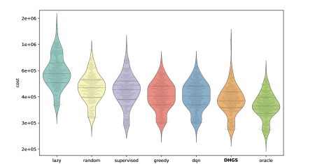
Figure 1: A violin plot comparing the total cost objective of the different solvers over all 250 instances. Each grey point represents an instance and its total cost for the corresponding solver. For each solver, the violin plot shows the distribution of the points, with horizontal lines marking the median and the $1^{st}$ and $3^{rd}$ quartiles.

To conclude, the results demonstrate that the adapted DHGS algorithm can perform favorably against different baselines, providing an effective general method for DVRPTW that does not require any pre-training. However, the dependency of DVRPTW on online data also makes it a natural test case for the application of machine learning. The results show that this is not straightforward. The supervised baseline, although trained on the oracle results, performs worse than the trivial greedy strategy. The reinforcement learning baseline dqn effectively learned the greedy strategy.

However, many of the top performing solvers in the competition were based on machine learning and demonstrate that more sophisticated approaches can successfully harness the potential of machine learning [3, 6, 9]. Some follow the simple scheme of applying HGS as a subroutine after performing ML-based customer selection. Hence, one interesting question for future research is if combining these ideas with DHGS can improve performance and robustness further.

References

- [1] Archetti, C., Carpenter, T., Kullman, N., McGeoch, C., Mendoza, J., Pardalos, P., Resende, M., Uchoa, E., Vidal, T.: The 12th DIMACS Challenge: Capacitated Vehicle Routing Problem with Time Windows. http://dimacs.rutgers.edu/programs/challenge/vrp/ (2022)
- [2] Costa, L., Contardo, C., Desaulniers, G.: Exact Branch-Price-and-Cut Algorithms for Vehicle Routing. Transportation Science 53(4), 946–985 (Jul 2019). https://doi.org/10.1287/trsc.2018.0878
- [3] Jungel, K., Baty, L., Klein, P.: Structured learning for the euro meets neurips 2022 vehicle routing competition. https://github.com/ortec/euro-neurips-vrp-2022-quickstart/blob/main/papers/Kleopatra.pdf (2022)
- [4] Kool, W., Bliek, L., Numeroso, D., Reijnen, R., Afshar, R.R., Zhang, Y., Catshoek, T., Tierney, K., Uchoa, E., Vidal, T., Gromicho, J.: The EURO Meets NeurIPS 2022 Vehicle Routing Competition (2022), https://euro-neurips-vrp-2022.challenges.ortec.com/
- [5] Kool, W., Juninck, J.O., Roos, E., Cornelissen, K., Agterberg, P., van Hoorn, J., Visser, T.: Hybrid Genetic Search for the Vehicle Routing Problem with Time Windows: A High-Performance Implementation (2022)
- [6] Kwon, Y.D., Choo, J., Bae, D., Kim, J., Hottung, A.: Cost shaping via reinforcement learning for vehicle routing problems. https://github.com/ortec/euro-neurips-vrp-2022-quickstart/blob/main/papers/Team_SB.pdf (2022)
- [7] Oliver, I.M., Smith, D.J., Holland, J.R.C.: A study of permutation crossover operators on the traveling salesman problem. In: Proceedings of the Second International Conference on Genetic Algorithms on Genetic Algorithms and Their Application. pp. 224–230. L. Erlbaum Associates Inc., USA (Oct 1987)
- [8] Pecin, D., Contardo, C., Desaulniers, G., Uchoa, E.: New Enhancements for the Exact Solution of the Vehicle Routing Problem with Time Windows. INFORMS Journal on Computing 29(3), 489–502 (Aug 2017). https://doi.org/10.1287/ijoc.2016.0744
- [9] Reese, B.M., Harenberg, S., Ladanyi, L., Pratt, R., Xu, Y.: Hybrid genetic search improvements for the euro meets neurips 2022 vehicle routing competition. https://github.com/ortec/euro-neurips-vrp-2022-quickstart/blob/main/papers/MilesToGoBeforeWeSleep.pdf (2022)
- [10] Vidal, T.: Technical Note: Split Algorithm in O(n) for the Capacitated Vehicle Routing Problem. Computers & Operations Research 69, 40–47 (May 2016). https://doi.org/10.1016/j.cor.2015.11.012
- [11] Vidal, T.: Hybrid genetic search for the CVRP: Open-source implementation and SWAP* neighborhood. Computers & Operations Research 140, 105643 (Apr 2022). https://doi.org/10.1016/j.cor.2021.105643
- [12] Vidal, T., Crainic, T.G., Gendreau, M., Lahrichi, N., Rei, W.: A Hybrid Genetic Algorithm for Multidepot and Periodic Vehicle Routing Problems. Operations Research 60(3), 611–624 (Jun 2012). https://doi.org/10.1287/opre.1120.1048
- [13] Vidal, T., Crainic, T.G., Gendreau, M., Prins, C.: A unified solution framework for multi-attribute vehicle routing problems. European Journal of Operational Research 234(3), 658–673 (May 2014). https://doi.org/10.1016/j.ejor.2013.09.045