Recognition of Mental Adjectives in An Efficient and Automatic Style

Abstract

In recent years, commonsense reasoning has received more and more attention from academic community. We propose a new lexical inference task, Mental and Physical Classification (MPC), to handle commonsense reasoning in a reasoning graph. Mental words relate to mental activities, which fall into six categories: Emotion, Need, Perceiving, Reasoning, Planning and Personality. Physical words describe physical attributes of an object, like color, hardness, speed and malleability. A BERT model is fine-tuned for this task and active learning algorithm is adopted in the training framework to reduce the required annotation resources. The model using ENTROPY strategy achieves satisfactory accuracy and requires only about 300 labeled words. We also compare our result with SentiWordNet to check the difference between MPC and subjectivity classification task in sentiment analysis.

1 Introduction

In the field of artificial intelligence, commonsense reasoning refers to the capacity that a machine understands the nature of scenes commonly encountered by humans every day, and makes reasonable and appropriate reactions, mimicking human cognitive abilities. Through commonsense reasoning, humans are capable of intricate reasoning relating to fundamental domains including time, space, naive physics, and naive psychology [6]. Therefore, a good starting point is understanding how time, space, naive physics affect human’s mind, exploring possible causal relationships. For example, let’s consider a review "This saltwater taffy had great flavors and was very soft and chewy. I loved it and I would highly recommend this candy!". The concepts "great flavors", "soft", "chewy" describe physical attributes of the saltwater taffy and the concepts "love", "recommend" describe mental activities of the reviewer. Here concept refers to word or phrase in natural language. If a seven years old child reads this review, the child would understand that the mental activities are caused by the taffy’s physical attributes. Figure 1 shows a possible reasoning graph existed in the child’s mind. The words "great flavors", "soft", "chewy" indicate that this taffy is edible with a positive effect. This effect greatly satisfies the reviewer’s need of food and then this strong satisfaction invokes the reviewer’s emotion of love with an reaction "I love it". That strong satisfaction also invokes the reviewer’s need of friendship positively, with an reaction that the reviewer would like to share this taffy with friends.

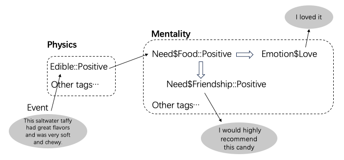
Figure 1: A reasoning graph between a physical event and mental reactions. Edible::Positive means positive effect over a physical attribute Edible. In mentality part, Need$Food::Positive, Need$Friendship::Positive mean positive effect over Food and Friendship respectively, which belong to Need category [17]. Need$Food::Positive invokes Love belonging to Emotion category [20]. Other tags not invoked are omitted.

To let a machine figure out a similar reasoning graph, the first step is recognizing which concept is Physical and which one is Mental. Then all concepts are mapped to numerous more granular tags, like Edible::Positive or Need$Friendship::Positive shown in Figure 1. Last, all tags are linked together to form a powerful reasoning graph. The first step cannot be skipped because the coarsest reasoning path, Physical -> Mental, provides causal concept pairs, facilitating design of more fine-grained tags. Under this research plan, we propose a task of Mental and Physical Classification (MPC) at lexical level in this work. Each adjective extracted from Amazon Fine Food Reviews dataset [18] is inferred with a binary tag, Mental or Physical, by a fine-tuned BERT model. A Mental adjective describes mental activities, like emotion, need, reasoning, while a Physical one shows physical attributes of an object, like color, hardness, speed and malleability. Although our inference methods have been for adjectives, they can be directly applied to other word classes. The inferred tags of MPC only reveals that an adjective is more likely to express a mental view or a physical view, as a word might have different senses.

Besides MPC, dozens of binary or multi-value tags, like Emotion or Need category will be developed in the follow-up research work. Moreover, in order to improve the reasoning performance, these tags might need to be updated or new tags join the reasoning graph. This continuous and rapid iterative process makes it impossible to annotate all the words at once. In fact, what this project really needs is the ability to tag all the words automatically relying on zero or very low annotation resources. Therefore, we consider active learning methods to train a BERT [7] model for MPC in this work. ENTROPY [13], CORESET [25], CAL [16] and Random strategies are implemented and evaluated. The experiment results indicate that ENTROPY outperforms others and achieves Mental F1 0.72 and Physical F1 0.87 on testset, with only around 300 words are annotated for training.

The definition of MPC task bears some similarity to subjectivity classification which is one task of sentiment analysis [14], and classify whether a piece of text is objective or subjective. To investigate the difference between these tasks, our result by ENTROPY is compared with SentiWordNet [24; 2]. We find that 41.5% of the Mental adjectives bear objective meanings, which indicates the notion of MPC is quite different from subjectivity classification. Adjective examples are listed out to illustrate this difference in Table 4.

The main contributions of this paper include the following three points: (1) a new task MPC is proposed to handle commonsense reasoning, (2) active learning is introduced to solve MPC efficiently, relying on only a small size of annotated words, (3) a dataset with the inferred MPC tags is released publicly for future research.

2 Related Work

Commonsense Reasoning. Reasoning between mentality and physics has been studied by the research community in recent years. The mental reason of affective events is explained based on seven common human needs [8]. Event2Mind studies two kind of mental state, intent and emotion, which are inferred by deep learning models given physical events described by short text-free phrases [22]. ATOMIC considers two more kind of mental state, planning and personality, under the same task setting of Event2Mind [23]. Reasoning between physical events are studied by [36] and [33]. Previous works provide no clear explanation about "how" and "why" in commonsense reasoning, which is the core question that our research works try to address.

Sentiment Analysis. Subjectivity classification and sentiment classification are two sub-topics of sentiment analysis [14]. Subjectivity classification is to determine whether a content is objective or subjective. On the other hand, sentiment classification is utilized for subjective content to identify the sentiment polarity, that is, whether the author expresses a positive or negative opinion. One approach to sentiment analysis is using lexicons where each word is assigned with scores showing it is neutral, positive or negative [32; 10; 11; 31]. These scores are known as prior polarity, that is, irrespective of the context, whether the word convey a positive or negative or neutral connotation [35]. One popular lexical resource is SentiWordNet [24; 2] which associates polarity scores to each synset of WordNet [19]. Early researches in this domain focus on adjectives, as adjectives express the majority of subjective meaning in a piece of writing [11; 31]. Under the same consideration, we also focus on adjectives for MPC first in this work.

Active Learning. When machine learning or deep learning algorithms are considered to solve NLP tasks, one of most common challenges is lack of labeled data and limited annotation resources due to project budget. To efficiently make use of annotation resources, only the most valuable samples are hoped to be selected out for human labeling. Active learning provides a set of algorithms to fulfill this goal [26]. ENTROPY is an uncertainty-based method, choosing the sample with the highest predicted entropy [13]. However, the problem with this approach is that there is a risk of picking outliers or similar samples [26]. To increase diversity of the selected samples, CORESET [25] chooses the furthest sample in the embedding space from the samples already selected in previous iterations. CAL [16] finds the most contrastive sample to its nearest neighbors by calculating KL divergence, leveraging both uncertainty and diversity.

BERT. In recent years BERT [7] has become one of the most famous pre-training language models and has shown effectiveness in many natural language processing tasks. These include sentiment analysis [28], semantical similarity [9], question answering [21] and entailment inference [34]. BERT is pre-trained on the BooksCorpus (800M words) [38] and English Wikipedia (2,500M words). By pre-training on such large text data, BERT grasps rich semantic information. The most common usage of BERT is fine-tuning it over downstream tasks, trained with data from downstream tasks to update all its pre-trained parameters. By this way, both the rich semantic information from pre-training and the features from downstream tasks are taken advantage of to achieve an excellent performance.

3 Data and Annotation

Task Definition. In this work, we define a binary classification task, inferring a word is Mental or Physical. The notion of Mental relates to mental activities, which fall into six categories: Emotion, Need, Perceiving, Reasoning, Planning and Personality. Personality are regarded as the external manifestation of persistent mental activities. Detailed definition of each category and word examples are shown in Table 4. Other words are defined as Physical describing physical attributes of an object, like color, hardness, speed and malleability. Mental words usually have abstract meanings, but Physical words have more concrete meanings that can be observed in the world. This difference can be used as a simple reference to determine which class a word belongs to. The inferred class only reveals that a word is more likely to express a mental view or a physical view, as a word might have different senses. The main reason we choose lexical level rather than sense level for MPC, is to facilitate subsequent research and reduce development complexity.

Data Process. Amazon Fine Food Reviews dataset [18] is used as corpus for MPC task, as this dataset contains reasoning between physics (food description) and mentality (people’s opinion) in our daily life. It has more than 0.5 million reviews of Amazon fine foods from Oct 1999 to Oct 2012. We use only text column and remove all other columns like ProductId, UserId, ProfileName for anonymization considerations. Data process contains three steps. An processing example is given in Table 1. First, each piece of review is splitted into words and each word is classified into part of speech (POS-tagging) . Then (adjective, noun) pairs are recognized and extracted out, where the noun appeared immediately after the adjective in review sentences. The goal of this step is to make sure the extracted adjectives are used in daily life to describe objects or states, like "roasted beans", "angry complaint", and counteract possible errors from POS-tagging. Finally, adjectives from these pairs are validated by checking if they have definition text from WordNet. After deduplication, 7292 adjectives are obtained. We use version 3.6.7 of NLTK package for POS-tagging and WordNet calling.

Review: I have found them all to be of good quality.
Step 1: Pos-tagging. Result: ("I", "PRP"), ("have", "VBP"), ("found", "VBN"), ("them", "PRP"), ("all", "DT"), ("to", "TO"), ("be", "VB"), ("of", "IN"), ("good", "JJ"), ("quality", "NN"), (".", ".")
Step 2: Detect (adjective, noun) pairs. Result: ("good", "quality")
Step 3: Validate adjectives. Result: "good"

Table 1: Review process pipeline. Input is "I have found them all to be of good quality." and after processing the word "good" is outputted.

Annotation. Each adjective is annotated by two annotators checking word definition from WordNet, and disagreements are adjudicated by another expert. All participants are experienced volunteers and they are notified how their annotations are used in this work. Examples of words and their definitions are presented in Appendix A. For words with different senses, annotation results are mainly based on the frequency of daily use. For instance, although the word "cold" has a Mental sense, "feeling or showing no enthusiasm", it’s labeled as Physical since it is used more frequently with the gloss "having a low or inadequate temperature or feeling a sensation of coldness or having been made cold by e.g. ice or refrigeration".

A testset consisting of 100 words is annotated for measuring model performance. It contains 26% Mental words and 74% Physical words. Among the Mental words, 12% of them have annotation disagreements while this number drops to 5% for Physical words. This difference indicates that Mental words are more likely to be misclassified. Total disagreement over this dataset between two annotators is 7% . Statistics of the testset is summarized in Table 2. For each active learning strategy, a dataset for training and validation is annotated, which has no overlap with the testset.

Class	Total	Disagreement	Rate
Mental	26	3	12%
Physical	74	4	5%

Table 2: Total word numbers, disagreement numbers and rate of disagreement of the two classes in the testset. Difference of disagreement rates indicates that Mental words are more likely to be misclassified.

4 Methods

We use active learning framework to train a binary classifier for MPC task, which is shown in Algorithm 1. An unlabeled word pool $\mathcal{U}$ is set up consisting of the extracted adjectives. The random strategy is used to select a word for annotation in the first iteration, while in other iterations different active learning strategies are used. We aim to annotate $K_{1}$ positives and $K_{2}$ negatives in each iteration, which are put into a labeled word pool $\mathcal{D}_{labeled}$. A threshold $M$ is set to control the total number of annotation of each iteration, in case that the active learning strategy fails to find another positive or negative sample. At the end of each iteration, a BERT model is fine-tuned over $\mathcal{D}_{labeled}$. When iterations end, the BERT model with best performance over testset is employed in pipeline for inference.

Algorithm 1 Active Learning Framework

0:  Unlabeled word pool $\mathcal{U}$, number of positive samples $K_{1}$ and negative samples $K_{2}$ and maximum annotated samples $M$ per iteration, number of iterations $T$

1:  $\mathcal{D}_{labeled}=\{\}$

2:  $t=0$

3:  while  $t<T$  do

4:     $\mathcal{D}_{pos},\mathcal{D}_{neg}=\{\},\{\}$

5:     $m=0$

6:     while True do

7:        if $t=1$ then

8:           $w_{new}\leftarrow$ Randomly select a word from $\mathcal{U}$

9:        else

10:           $w_{new}\leftarrow$ Select a word from $\mathcal{U}$ by a specific strategy

11:        end if

12:        Annotate $w_{new}$ with a class label $C$

13:        $\mathcal{U}=\mathcal{U}\setminus\{w_{new}\}$

14:        $m=m+1$

15:        if $C$ is positive and $|\mathcal{D}_{pos}|<K_{1}$ then

16:           $\mathcal{D}_{pos}=\mathcal{D}_{pos}\cup\{(w_{new},C)\}$

17:        end if

18:        if $C$ is negative and $|\mathcal{D}_{neg}|<K_{2}$ then

19:           $\mathcal{D}_{neg}=\mathcal{D}_{neg}\cup\{(w_{new},C)\}$

20:        end if

21:        if ($|\mathcal{D}_{pos}|=K_{1}$ and $|\mathcal{D}_{neg}|=K_{2}$) or $m=M$ then

22:           break

23:        end if

24:     end while

25:     $\mathcal{D}_{labeled}=\mathcal{D}_{labeled}\cup\mathcal{D}_{pos}\cup\ \mathcal{D}_{neg}$

26:     Fine-tune a BERT over $\mathcal{D}_{labeled}$

27:     $t=t+1$

28:  end while

BERT fine-tuning and inference procedure is shown in Figure 2. As WordNet maps words into sets of cognitive synonyms, each expressing a distinct concept, therefore more than one piece of definition text are provided by WordNet for a given word. For example, "shining" belongs to three clusters as an adjective with three different definitions: (1) marked by exceptional merit, (2) made smooth and bright by or as if by rubbing; reflecting a sheen or glow, and (3) reflecting light. All of them are aggregated as one piece of text, serving as input of BERT with a special token [CLS] at head. We use the final hidden state of [CLS] as BERT output, which is then connected with a dropout layer [29] and a linear layer. Sigmoid node is added after the linear layer to transform logits into the probability of positive class. For fine-tuning, a standard cross entropy loss is computed to update all parameters of the BERT model and the subsequent linear layer.

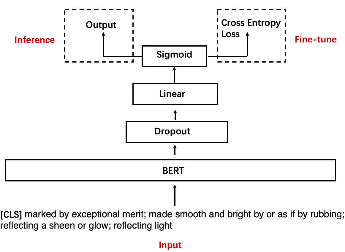
Figure 2: Definitions of words are concatenated with [CLS] at head as input of BERT. A dropout and a linear layer are connected to BERT sequentially. At last, a sigmoid node outputs the probability of being positive. The output probability is consumed for inference, or as input of cross entropy loss for fine-tuning. We use a word "shining" with its definition text as an input example.

5 Experiments and Results

We compare four active learning strategies, considering their classification performance and annotation resource consumption, to find which strategy is most suitable for MPC task given a limited project budget. Mental class serves as positive and Physical serves as negative in training. F1 scores of Mental and Physical classes over testset are computed respectively. The average of the number of labeled samples in each iteration is recorded.

ENTROPY. Samples with the highest predicted entropy are selected [13]. For binary classification, the closer the prediction probability of a sample is to 0.5, the higher its entropy is. Therefore, at the starting of each iteration, the BERT model from last iteration outputs the probability of all the words in $\mathcal{U}$ and the word whose probability is closest to 0.5 is selected.

CORESET. Samples that are furthest away from the samples selected in previous iterations are chosen to enlarge the semantic diversity [25]. FastText [3] is used to represent a word by embedding vector, as fastText works well in word-level semantic textual similarity (STS) tasks [37]. In each iteration, a word is selected as follows:

$$w_{new}=\mathop{\arg\max_{w\in\mathcal{U}}}{\mathop{\min_{v\in\mathcal{D}_{labeled}}}{L_{2}(\phi(w),\phi(v))}},$$ (1)

where $L_{2}(\cdot,\cdot)$ computes $L_{2}$ distance between two vectors and $\phi(\cdot)$ returns the embedding vector of a word.

The most contrastive sample to its nearest neighbors by calculating KL divergence is chosen.

CAL. The most contrastive sample to its nearest neighbors by calculating KL divergence is chosen [16]. Given a word $w$ in unlabeled word pool $\mathcal{U}$, nearest 10 words are selected as neighbors in labeled word pool $\mathcal{D}_{labeled}$ by $L_{2}$ distance. The average KL divergence between $w$ and its neighbors is computed as a measure of contrastive degree. The word with the largest value of this measure is selected.

Random. Select a word $w$ in unlabeled word pool $\mathcal{U}$ randomly.

(a) Mental F1

Iteration	ENTROPY	CORESET	CAL	Random
3	0.61	0.69	0.62	0.61
4	0.72	0.71	0.64	0.64
5	0.70	0.69	0.68	0.64

(b) Physical F1

Iteration	ENTROPY	CORESET	CAL	Random
3	0.82	0.66	0.79	0.71
4	0.87	0.83	0.80	0.66
5	0.85	0.81	0.76	0.69

Table 3: Averaged F1 scores after 3,4,5 iterations. ENTROPY outperforms the other three, achieving the highest Mental F1 0.72 and Physical F1 0.87 at iteration 4.

All strategies share the same experimental settings as following: total iterations $T$ = 5, number of positive samples $K_{1}$ = 20, number of negative samples $K_{2}$ = 20, maximum annotation number $M$ = 120. In each iteration, BERT fine-tuning takes totally 20 epochs with learning rate 2e-5 and batch size 32. Learning rate drops to 1/10 of the original level after 10 epochs. We split $\mathcal{D}_{labeled}$ by 80% - 20% as trainset and devset. If BERT outputs a value greater than 0.5, the word is considered to belong to Mental, otherwise Physical. Winner model $\mathcal{M}_{t}$ is the one with maximum accuracy over devset. We hypertune BERT with different values of learning rate {1e-5, 2e-5, 1e-4} and batch size {32, 64, 128} for ENTROPY strategy. The best result over devset is achieved at 2e-5 learning rate and 32 batch size.

Our BERT implementation is provided by Hugging Face and we choose "bert-base-uncased" version which contains 110M parameters and does not make a difference between lowercase and uppercase words. We use the Adam optimizer with 0.001 weight decay [15]. The size of the linear layer is 768 which is the same size of BERT final hidden state. Dropout with a probability of 0.3 is applied in the network. Training framework is based on Pytorch Lightning (version 1.5.8) which could greatly boosts training efficiency. All experiments use this network architecture.

Category	Definition	Example
Emotion	Plutchik’s wheel of emotions [20].	favored, scorned, frisky, trustworthy, gripping, stilted
Need	Maslow’s hierarchy of needs [17].	devout, deserving, protective, hired, wealthy, rewarding
Perceiving	individuals use information to form perceptions of themselves and others based on social categories. [1].	sensuous, ubiquitous, instinctive, detected, recognized, perceivable
Reasoning	Deduction based on classical logic [27] or mental models [12].	suitable, predominate, critical, substandard, relevant, causal
Planning	Mental time travel [30].	committed, aimless, exploited, unplanned, purposeful, executed
Personality	Stable patterns of behavior, cognition, and emotion [4].	whimsical, squeamish, shy, punctual, entrepreneurial, intrepid

Table 4: Mental adjective examples which are classified as objective in subjectivity classification. The definition of each mental category is provided.

Each strategy is run three times with different random seeds and the averaged F1 scores over testset after three, four, five iterations are reported in Table 3. ENTROPY outperforms the other three, achieving the highest Mental F1 0.72 and Physical F1 0.87 at iteration 4. The reason that CAL fails might be we don’t find semantically similar neighbors as the size of $\mathcal{D}_{labeled}$ is too small. Table 5 shows annotation resource consumption. ENTROPY requires 60~70 labeled words per iteration, which means totally only 300 labeled words are needed to deliver an applicable classifier. CORESET and Random need more annotations than ENTROPY. CAL could not provide enough positive and negative samples after 120 words are annotated for some iterations. Precision and recall scores are presented in Appendix B.

Strategy	Words/Iter	EnoughSamples
ENTROPY	60 ~ 70	Yes
CORESET	80 ~ 120	Yes
CAL	50 ~ 120	No
Random	80 ~ 100	Yes

Table 5: Range of annotation number per iteration. ENTROPY requires the lowest annotation resource. CAL could not provide enough positive and negative samples after 120 words are annotated for some iterations.

6 Comparison with SentiWordNet

As the notion of Mental and Physical is to some extent similar to "subjective" and "objective" in the subjectivity classification task [14] of sentiment analysis, we’d like to investigate the difference between them. We choose to compare our result with SentiWordNet [24; 2] which is the most used lexicon in social opinion mining studies [5]. SentiWordNet is a lexical resource which labels each synset from WordNet [19] as "positive", "negative" or "neutral". The used version of SentiWordNet is 3.0, which is based on WordNet 3.0.

SentiWordNet 3.0 associates each synset with three numerical scores PosScore, NegScore and ObjScore which show how positive, negative, and neutral the words contained in the synset are [2]. All three scores range from 0 to 1 and their sum is 1. We focus on adjective synsets and classify each of them into two classes: SubSyn, if the maximum of the three scores is PosScore or NegScore; otherwise, ObjSyn. For an adjective that belongs to more than one synset, it owns different senses, perhaps having both subjective and objective meanings. Therefore, at lexical level, an adjective is labeled by this rule: Subjective, if it only belongs to SubSyn synsets; Objective, if it only belongs to ObjSyn synsets; Dual, if if belongs to both SubSyn and ObjSyn synsets. Table 6 shows the distribution of Subjective, Objective and Dual adjectives in Mental and Physical classes. We find that 43% of the Mental adjectives are labeled as Objective. This indicates the notions of Mental/Physical are different from Subjective/Objective. In fact, many Objective adjectives bear mental functionalities. Some adjective examples are listed to illustrate this point in Table 4 in six categories: Emotion, Need, Perceiving, Reasoning, Planning and Personality.

Class	Subjective	Objective	Dual	Total
Mental	28%	43%	29%	100%
Physical	9%	74%	17%	100%

Table 6: Distribution of Subjective, Objective and Dual adjectives in Mental and Physical classes. Only 28% of those words in Mental fall into Subjective, while 43% belong to Objective. This indicates many Objective adjectives bear mental functionalities under MPC definition.

7 Conclusion

Aiming to explicitly reveal reasoning path in commonsense scenarios, our first step is to classify a word into Mental or Physical. We provide clear definitions of these two categories and a simple criterion for judging them. Active learning algorithm is implemented to fine-tune a BERT model, reducing the required annotation resources. The BERT model automatically infers which class an adjective belongs to. We release the inferred tags publicly to facilitate future research. We also compare our result with SentiWordNet, and find the notions of Mental/Physical is different from Subjective/Objective in sentiment analysis. Many Objective adjectives bear mental functionalities under MPC definition.

Future research works focus on designing more fine-grained tags and training models to automatically infer them over words. Links are built between tags in a manual way or machine-learning style, to form an applicable reasoning graph. We hope to translate what humans know about the world and about themselves into graph that will improve the intelligence of machines. Large language models (LLMs) provide powerful techniques to extract data patterns in nature language, which makes it possible to perfectly associate words with all kinds of human-designed tags. However, at the level of reasoning, relying on LLMs is not necessarily feasible, and painstaking manual work may be essential.

Limitations

Although the model by ENTROPY achieves acceptable F1 scores, there’s still a lot of room for improvement of classification precision and recall. For example, use more annotated words for fine-tuning, or try other deep learning algorithms. We leave this optimization in the future after we verify the whole research plan becomes feasible and the classification performance is a bottleneck for commonsense reasoning ability.

As a word has different meanings in different contexts, the best granularity for MPC is gloss level rather than lexical level. That’s to say, use each piece of gloss text as BERT input instead of merging all glosses of a word into one piece of text. Then, the output shows if a gloss belongs to Mental or Physical. However, lexical level facilitate the development of reasoning graph as there’s no need to consider context. We will change to gloss level by the time it’s verified that context becomes a bottleneck and it should be integrated into reasoning graph.

Appendix A Word examples in MPC task

Table 7 shows seven adjectives with their classes in MPC task. From these examples, we could see clear difference in definition texts between Mental and Physical classes. Therefore, it’s possible to fine-tune a high-accuracy BERT for MPC task.

Word	Class	Definition
interested	Mental	having or showing interest; especially curiosity or fascination or concern; involved in or affected by or having a claim to or share in;
angry	Mental	feeling or showing anger; (of the elements) as if showing violent anger; severely inflamed and painful;
clever	Mental	showing self-interest and shrewdness in dealing with others; mentally quick and resourceful;
lazy	Mental	moving slowly and gently; disinclined to work or exertion;
molecular	Physical	relating to or produced by or consisting of molecules; relating to simple or elementary organization;
blue	Physical	of the color intermediate between green and violet; having a color similar to that of a clear unclouded sky;
automated	Physical	operated by automation;

Table 7: Examples of words and their classes in MPC task. Definitions are provided by WordNet. From these examples, we could see clear difference in definition texts between two classes.

Appendix B Precision and Recall

Table 8 shows averaged precision and recall after 3,4,5 iterations of each strategy. For Mental class, ENTROPY achieves the highest precision around 0.8 and CAL has the highest recall above 0.9. For Physical class, CAL achieves the highest precision above 0.9 and ENTROPY has the highest recall around 0.9.

(a) Mental Precision

Iteration	ENTROPY	CORESET	CAL	Random
3	0.70	0.62	0.53	0.54
4	0.81	0.63	0.51	0.72
5	0.79	0.59	0.54	0.69

(b) Mental Recall

Iteration	ENTROPY	CORESET	CAL	Random
3	0.54	0.79	0.74	0.73
4	0.65	0.81	0.87	0.57
5	0.64	0.82	0.94	0.61

(c) Physical Precision

Iteration	ENTROPY	CORESET	CAL	Random
3	0.77	0.86	0.81	0.79
4	0.82	0.87	0.88	0.79
5	0.82	0.88	0.94	0.79

(d) Physical Recall

Iteration	ENTROPY	CORESET	CAL	Random
3	0.87	0.73	0.64	0.60
4	0.91	0.73	0.53	0.88
5	0.90	0.68	0.55	0.83

Table 8: Averaged precision and recall of Mental and Physical after 3,4,5 iterations.

References

[1]
Saks Alan and J Gary.
Perception, attribution, and judgment of others.
Organizational behaviour: Understanding and managing life at
work, 7:1–20, 2011.
[2]
Stefano Baccianella, Andrea Esuli, Fabrizio Sebastiani, et al.
Sentiwordnet 3.0: an enhanced lexical resource for sentiment analysis
and opinion mining.
In Lrec, volume 10, pages 2200–2204, 2010.
[3]
Piotr Bojanowski, Edouard Grave, Armand Joulin, and Tomas Mikolov.
Enriching word vectors with subword information.
arXiv preprint arXiv:1607.04606, 2016.
[4]
Philip J Corr and Gerald Ed Matthews.
The Cambridge handbook of personality psychology.
Cambridge University Press, 2020.
[5]
Keith Cortis and Brian Davis.
Over a decade of social opinion mining: a systematic review.
Artificial intelligence review, 54(7):4873–4965, 2021.
[6]
Ernest Davis and Gary Marcus.
Commonsense reasoning and commonsense knowledge in artificial
intelligence.
Communications of the ACM, 58(9):92–103, 2015.
[7]
Jacob Devlin, Ming-Wei Chang, Kenton Lee, and Kristina Toutanova.
Bert: Pre-training of deep bidirectional transformers for language
understanding.
arXiv preprint arXiv:1810.04805, 2018.
[8]
Haibo Ding, Tianyu Jiang, and Ellen Riloff.
Why is an event affective? classifying affective events based on
human needs.
In AAAI Workshops, 2018.
[9]
Bill Dolan and Chris Brockett.
Automatically constructing a corpus of sentential paraphrases.
In Third International Workshop on Paraphrasing (IWP2005),
2005.
[10]
Vasileios Hatzivassiloglou and Kathleen McKeown.
Predicting the semantic orientation of adjectives.
In 35th annual meeting of the association for computational
linguistics and 8th conference of the european chapter of the association for
computational linguistics, pages 174–181, 1997.
[11]
Minqing Hu and Bing Liu.
Mining and summarizing customer reviews.
In Proceedings of the tenth ACM SIGKDD international conference
on Knowledge discovery and data mining, pages 168–177, 2004.
[12]
Philip N Johnson-Laird.
Mental models and deduction.
Trends in cognitive sciences, 5(10):434–442, 2001.
[13]
David D Lewis.
A sequential algorithm for training text classifiers: Corrigendum and
additional data.
In Acm Sigir Forum, volume 29, pages 13–19. ACM New York, NY,
USA, 1995.
[14]
Bing Liu et al.
Sentiment analysis and subjectivity.
Handbook of natural language processing, 2(2010):627–666,
2010.
[15]
Ilya Loshchilov and Frank Hutter.
Decoupled weight decay regularization.
arXiv preprint arXiv:1711.05101, 2017.
[16]
Katerina Margatina, Giorgos Vernikos, Loïc Barrault, and Nikolaos Aletras.
Active learning by acquiring contrastive examples.
arXiv preprint arXiv:2109.03764, 2021.
[17]
Abraham Harold Maslow.
A theory of human motivation.
Psychological review, 50(4):370, 1943.
[18]
Julian John McAuley and Jure Leskovec.
From amateurs to connoisseurs: modeling the evolution of user
expertise through online reviews.
In Proceedings of the 22nd international conference on World
Wide Web, pages 897–908, 2013.
[19]
George A Miller.
Wordnet: a lexical database for english.
Communications of the ACM, 38(11):39–41, 1995.
[20]
Robert Plutchik.
A general psychoevolutionary theory of emotion.
In Theories of emotion, pages 3–33. Elsevier, 1980.
[21]
Pranav Rajpurkar, Jian Zhang, Konstantin Lopyrev, and Percy Liang.
SQuAD: 100,000+ questions for machine comprehension of text.
In Proceedings of the 2016 Conference on Empirical Methods in
Natural Language Processing, pages 2383–2392, Austin, Texas, November 2016.
Association for Computational Linguistics.
[22]
Hannah Rashkin, Maarten Sap, Emily Allaway, Noah A. Smith, and Yejin Choi.
Event2mind: Commonsense inference on events, intents, and reactions.
In Annual Meeting of the Association for Computational
Linguistics, 2018.
[23]
Maarten Sap, Ronan Le Bras, Emily Allaway, Chandra Bhagavatula, Nicholas
Lourie, Hannah Rashkin, Brendan Roof, Noah A. Smith, and Yejin Choi.
Atomic: An atlas of machine commonsense for if-then reasoning.
In AAAI Conference on Artificial Intelligence, 2019.
[24]
Fabrizio Sebastiani and Andrea Esuli.
Sentiwordnet: A publicly available lexical resource for opinion
mining.
In Proceedings of the 5th international conference on language
resources and evaluation, pages 417–422. European Language Resources
Association (ELRA) Genoa, Italy, 2006.
[25]
Ozan Sener and Silvio Savarese.
Active learning for convolutional neural networks: A core-set
approach.
arXiv preprint arXiv:1708.00489, 2017.
[26]
Burr Settles.
Active learning literature survey.
2009.
[27]
Stewart Shapiro and Teresa Kouri Kissel.
Classical logic.
2000.
[28]
Richard Socher, Alex Perelygin, Jean Wu, Jason Chuang, Christopher D. Manning,
Andrew Ng, and Christopher Potts.
Recursive deep models for semantic compositionality over a sentiment
treebank.
In Proceedings of the 2013 Conference on Empirical Methods in
Natural Language Processing, pages 1631–1642, Seattle, Washington, USA,
October 2013. Association for Computational Linguistics.
[29]
Nitish Srivastava, Geoffrey Hinton, Alex Krizhevsky, Ilya Sutskever, and Ruslan
Salakhutdinov.
Dropout: a simple way to prevent neural networks from overfitting.
The journal of machine learning research, 15(1):1929–1958,
2014.
[30]
Thomas Suddendorf and Michael C Corballis.
The evolution of foresight: What is mental time travel, and is it
unique to humans?
Behavioral and brain sciences, 30(3):299–313, 2007.
[31]
Maite Taboada, Caroline Anthony, and Kimberly D Voll.
Methods for creating semantic orientation dictionaries.
In LREC, pages 427–432, 2006.
[32]
Maite Taboada, Julian Brooke, Milan Tofiloski, Kimberly Voll, and Manfred
Stede.
Lexicon-based methods for sentiment analysis.
Computational linguistics, 37(2):267–307, 2011.
[33]
Alon Talmor, Jonathan Herzig, Nicholas Lourie, and Jonathan Berant.
Commonsenseqa: A question answering challenge targeting commonsense
knowledge.
ArXiv, abs/1811.00937, 2019.
[34]
Adina Williams, Nikita Nangia, and Samuel R Bowman.
A broad-coverage challenge corpus for sentence understanding through
inference.
arXiv preprint arXiv:1704.05426, 2017.
[35]
Theresa Wilson, Janyce Wiebe, and Paul Hoffmann.
Recognizing contextual polarity in phrase-level sentiment analysis.
In Proceedings of Human Language Technology Conference and
Conference on Empirical Methods in Natural Language Processing, pages
347–354, Vancouver, British Columbia, Canada, October 2005. Association for
Computational Linguistics.
[36]
Rowan Zellers, Ari Holtzman, Yonatan Bisk, Ali Farhadi, and Yejin Choi.
Hellaswag: Can a machine really finish your sentence?
In Annual Meeting of the Association for Computational
Linguistics, 2019.
[37]
Vitalii Zhelezniak, Aleksandar Savkov, April Shen, and Nils Y. Hammerla.
Correlation coefficients and semantic textual similarity.
In North American Chapter of the Association for Computational
Linguistics, 2019.
[38]
Yukun Zhu, Ryan Kiros, Rich Zemel, Ruslan Salakhutdinov, Raquel Urtasun,
Antonio Torralba, and Sanja Fidler.
Aligning books and movies: Towards story-like visual explanations by
watching movies and reading books.
In Proceedings of the IEEE international conference on computer
vision, pages 19–27, 2015.