Entanglement of weighted graphs uncovers transitions in variable-range interacting models

Abstract

The cluster state acquired by evolving the nearest-neighbor (NN) Ising model from a completely separable state is the resource for measurement-based quantum computation. Instead of an NN system, a variable-range power law interacting Ising model can generate a genuine multipartite entangled (GME) weighted graph state (WGS) that may reveal intrinsic characteristics of the evolving Hamiltonian. We establish that the pattern of generalized geometric measure (GGM) in the evolved state with an arbitrary number of qubits is sensitive to fall-off rates and the range of interactions of the evolving Hamiltonian. We report that the time-derivative and time-averaged GGM at a particular time can detect the transition points present in the fall-off rates of the interaction strength, separating different regions, namely long-range, quasi-local and local ones in one- and two-dimensional lattices with deformation. Moreover, we illustrate that in the quasi-local and local regimes, there exists a minimum coordination number in the evolving Ising model for a fixed total number of qubits which can mimic the GGM of the long-range model. In order to achieve a finite-size subsystem from the entire system, we design a local measurement strategy that allows a WGS of an arbitrary number of qubits to be reduced to a local unitarily equivalent WGS having fewer qubits with modified weights.

I Introduction

The computational time of certain mathematical problems like prime factorization of integers Shor (1997) can be reduced utilizing the quantum mechanical principles compared to classically available algorithms – an important milestone that establishes the significance of building quantum computers Nielsen and Chuang (2010). Since then, quantum speedups that cannot be achieved by the best classical computer have been demonstrated in distinguishing classes of functions Deutsch and Jozsa (1992); Bernstein and Vazirani (1997) in a search problem from database Grover (1997) in estimating phases of an operator Kitaev (1995); Kitaev et al. (2002) and for solving linear systems of equations Harrow et al. (2009) to name a few. Although entanglement Horodecki et al. (2009) has been shown to be beneficial for accomplishing higher efficiency in certain quantum protocols, including various computational tasks Linden and Popescu (2001); Jozsa and Linden (2003); Van den Nest (2013) and quantum communication Ekert (1991); Bennett and Wiesner (1992); Bennett et al. (1992, 1993); Mattle et al. (1996); Jennewein et al. (2000); Gisin et al. (2002); Bennett and Brassard (2014); Ren et al. (2017); Guo et al. (2019), the resource required to attain quantum supremacy in quantum algorithms has yet to be determined Ahnefeld et al. (2022); Naseri et al. (2022).

On the other hand, entanglement is one of the prerequisites for measurement-based quantum computation (MBQC) Raussendorf and Briegel (2001); Hein et al. (2004, 2006); Casati et al. (2006); Browne and Briegel (2006); Briegel et al. (2009) which allows one to construct all the universal quantum gates required in a quantum computer Barenco et al. (1995). In the paradigm of MBQC or one-way quantum computation Raussendorf and Briegel (2001); Browne and Briegel (2006), generation of genuine multipartite entangled (GME) states and more specifically, multipartite cluster states Briegel and Raussendorf (2001); Yokoyama et al. (2013) remain crucial. These states are specific types of stabilizer states, known also as graph states, which are employed as a universal resource for measurement-based circuits followed by Clifford operations and they are easy to simulate through classical computer Aaronson and Gottesman (2004); Anders and Briegel (2006); Nielsen and Chuang (2010). The corresponding states have been successfully generated on several physical platforms and are used to show a variety of information processing tasks Zhang et al. (2006); Prevedel et al. (2007); Tame et al. (2007); Lanyon et al. (2013); Bell et al. (2013); Yokoyama et al. (2013); Bell et al. (2014a, b). Beyond one-way models, numerous kinds of universal resource states, such as two-dimensional ($2$D) cluster Briegel and Raussendorf (2001); Brell (2015), Affleck-Kennedy-Lieb-Tasaki (AKLT)-type Affleck et al. (1988), Toric code Kitaev (2003) and weighted graph states (WGS) Sen (De); Hartmann et al. (2007); Anders et al. (2007); Xue (2012) are also shown to be useful for quantum computation Gross et al. (2007); Gross and Eisert (2007).

The original proposal of producing cluster states, which are necessary for MBQC, solely employs nearest-neighbor Ising model Briegel and Raussendorf (2001). However, long-range (LR) quantum spin models are naturally created by neutral atoms in optical lattices interacting via dipole interactions Mamaev et al. (2019) or trapped ions Friedenauer et al. ; Kim et al. (2009); Khromova et al. (2012); Islam et al. (2011); Britton et al. (2012) under Coulomb potential Porras and Cirac (2004). Furthermore, such LR models frequently exhibit critical phenomena and possess phases that are not captured by short-range (SR) quantum spin models Koffel et al. (2012); Vodola et al. (2014, 2015); Defenu et al. (2020); Román-Roche et al. (2023); Kaicher et al. (2023). For instance, counter-intuitive results in LR models include breaking of the Mermin-Wagner-Hohenberg theorem Mermin and Wagner (1966); Hohenberg (1967); Peter et al. (2012), the rapid propagation of correlations Maghrebi et al. (2016); Gong et al. (2017); Ares et al. (2018, 2019), and violations of entanglement area law Eisert et al. (2010); Koffel et al. (2012); Schachenmayer et al. (2013); Cadarso et al. (2013). In addition, it has been demonstrated that on one hand, the ground or thermal states of the LR model possess a high multipartite entanglement or a more spreading of bipartite entanglement and on the other hand, multipartite entangled states can also be created through the LR models Koffel et al. (2012); Vodola et al. (2014); Ren et al. (2020); Lakkaraju et al. (2020, 2021, 2022); Francica and Dell’Anna (2022); Gong et al. (2023).

In this context, it is interesting to explore the properties of the dynamical state obtained via interacting LR spin systems and its suitability for MBQC, starting from a suitable product state. In particular, investigations have focused on the scaling of block entanglement, two-point correlation function, multipartite entanglement Sen (De); Biswas et al. (2014), and quantum discord Ollivier and Zurek (2001); Modi et al. (2012); Bera et al. (2017) of the state following evolution under the LR Ising model Dür et al. (2005); Mahto et al. (2022). Moreover, random quantum circuits implementation by carrying out measurements on weighted graph states Plato et al. (2008), and robust entanglement concentration protocol Frantzeskakis et al. (2023) for generating high-fidelity Greenberger–Horne–Zeilinger states Greenberger et al. (1989) have been proposed in the presence or absence of coherent and incoherent noise.

The genuine multipartite entanglement Meyer and Wallach (2002); Hashemi Rafsanjani et al. (2012); Sadhukhan et al. (2017); Gour and Yu (2018); Xie and Eberly (2021) of the dynamical state in various geometries and its characteristics under local measurements have not yet been addressed in the context of variable-range (VR) interactions included in the evolution Hamiltonian for one- and two-dimensional ($2$D) lattices. On one hand, these investigations can highlight the potential of the evolved state as a resource in quantum information protocols and identify phases and critical phenomena that are present in the evolution Hamiltonian. On the other hand, the impact of local measurements can indicate how to decouple certain parts of the circuits from the entire circuits, which can play a vital role on the performance of the computation. To accomplish this goal, we first show that the evolved state generated via VR interactions, referred to as weighted graph state, is genuinely multipartite entangled (GME) having nonvanishing generalized geometric measure Wei and Goldbart (2003) (GGM) Sen (De) and its pattern with time depends on the decay rate of interactions and the coordination number. Moreover, we know that the power-law decay in interactions of the LR transverse Ising model undergoes transitions from long-range to quasi-local and from quasi-local to local ones Koffel et al. (2012); Vodola et al. (2014, 2015); Defenu et al. (2020); Román-Roche et al. (2023); Kaicher et al. (2023). We report that the time-derivatives and time-averaged GME content of the WGSs can detect transitions, present in the fall-off rates in one- and two-dimensional lattices. More importantly, we demonstrate that if the $2$D square lattice is distorted with an arbitrary angle, resulting in a hexagonal lattice, the discontinuity in the derivative of the multipartite entanglement with respect to time or fall-off rate can predict the transition points in the decay rate of the evolving Hamiltonian. Further, we determine that there exist threshold values on the total number of qubits and coordination number above which the GME produced via VR interactions remains constant, thereby providing lower bounds on the number of two-qubit gates required to simulate the interacting Hamiltonian used for producing WGS. The results can be important during the realization of the WGS in laboratories e.g., with superconducting qubits Song et al. (2017a, b); Pedersen et al. (2019); Song et al. (2019).

Certain WGS with a minimal number of qubits may be necessary during the implementation of certain algorithms, and in such cases, the goal will be to generate WGS with a required number of qubits from the same state with an arbitrary number of qubits by making local measurements. For cluster state, such a measurement approach is well known Raussendorf et al. (2003). In this paper, we present a local measurement strategy that allows us to obtain local unitary equivalent WGS with adjusted weights.

The paper is structured in the following manner. In Sec. II, we introduce the exact expression of the WGS in various lattice geometries. The closed forms of GGM are calculated in Sec. III. Using the trends of GGM, detection of transitions in the fall-off rates of the evolution Hamiltonian is presented in Sec. IV while the investigations of emulating the GME in the LR model through the SR ones is examined in Sec. V. We discuss the impact of local measurements on the WGS in Sec. VI. The concluding remarks is included in Sec. VII.

II Generation of Weighted Graph State via long-range Hamiltonian with varying interaction strength

A weighted graph state of $N$ parties can be expressed by an underlying graph $G=(V,E)$, with the $N$ parties forming the set of vertices, $V=\{1,2,\ldots,N\}$ connected by a set of edges, $E\subset V\times V$ based on the interactions among the parties. The adjacency matrix of $G$ is $\Phi_{E}=(\phi_{ij})$, where the weight $\phi_{ij}$ denotes the interaction between the parties (vertices) $i$ and $j$. We consider real weights, i.e., $\Phi_{E}$ is real and symmetric matrix. Therefore the underlying graph $G$ is simple and undirected, i.e. $\phi_{ii}=0$ and $\phi_{ij}=\phi_{ji}\forall(i,j)\in V\times V$.

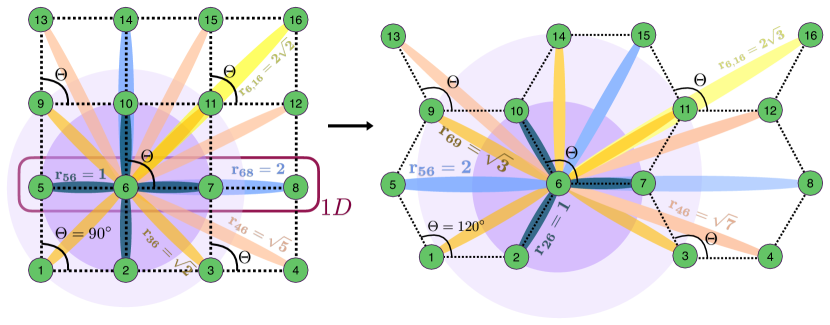
Figure 1: The two-dimensional lattice with sites $L\times L$ ($L=4$) can be transformed from square (left) to the honeycomb (right) lattice, forming fully connected weighted graph state with different $\Theta$ in open boundary condition. Connections are shown for a single qubit with the corresponding distances. $\Theta=90^{\circ}$ and $\Theta=120^{\circ}$ corresponds to the square and the honeycomb lattices respectively. Each site $\overrightarrow{\mathbf{i}}=(i_{x},i_{y})$ is indexed as $i=(i_{x}-1)*L+i_{y}$, where $i_{x}\in[1,L]$, $i_{y}\in[1,L]$ and $i_{x},i_{y}\in\mathbb{N}$ . Different colors (shades) signifies different strength of the interactions, which decreases with increasing distance.

To construct a spin-$\frac{1}{2}$ graph state, each vertex is a qubit initialized in $\ket{+}=(\ket{0}+\ket{1})/\sqrt{2}$, where $\ket{0}$ and $\ket{1}$ are the eigenstates of the Pauli matrix $\sigma_{z}$ with the corresponding eigenvalues $1$ and $-1$. Furthermore, two-qubit interacting unitary, $U_{ij}=e^{-iH_{ij}t}\forall i,j\in V$, acts on each vertices, entangling the pairs of qubits (creating the edges) which is achieved by the two-qubit Hamiltonian, $H_{ij}=\phi_{ij}\Big{(}\frac{1-\sigma_{z}^{(i)}}{2}\Big{)}\Big{(}\frac{1-\sigma_{z}^{(j)}}{2}\Big{)}$. Hence, the unitary transformation, in this case, takes the diagonal form as $U_{ij}=\text{diag}(1,1,1,e^{-ig_{ij}(t)})$, known as the controlled-phase gate with $g_{ij}(t)=\phi_{ij}t$. Here, $\phi_{ij}$, which comprises the information of the range and strength of the interaction, is constant throughout the time. Therefore, the total interacting Hamiltonian acting on the graph can be written as $H=\sum_{i=1}^{N-1}\sum_{j>i}^{N}H_{ij}$

Notice that the Hamiltonian remains unchanged under the exchange of two index, $H_{ij}=H_{ji}$ and $[H_{ij},H_{jk}]=0$, which satisfies the criteria for the graph having undirected and unordered edges respectively. Finally, the graph state for $N$-party system can be expressed as

$$\ket{\Psi_{G}(t)}_{N} = \prod_{i,j}U_{ij}(t)\ket{+}^{\otimes N}.$$ (1)

Considering only nearest neighbor interactions in $1$D, i.e., $H=\sum_{i}H_{i,i+1}$ and setting $\phi_{i,i+1}t=(2n-1)\pi$ for any $n\in\mathbb{N}$, (with $\mathbb{N}$ being the set of natural numbers) which transforms the edge connecting unitaries to be $U_{i,i+1}=\text{diag}(1,1,1,-1)\equiv\text{CNOT}$, we get the well known MBQC resource state, known as the cluster state Briegel and Raussendorf (2001) having the form, $\ket{\Psi_{G}((2n-1)\pi)}_{N}=\frac{1}{2^{N/2}}\bigotimes_{i=1}^{N}\big{(}\ket{0}_{i}+\ket{1}_{i}\sigma_{i+1}^{z}\big{)},$ using the convention that $\sigma_{N+1}^{z}=\mathbb{I}$ in the open boundary condition.

Instead of this simplified scenario, we concentrate on more general experimentally viable picture of all-to-all connectivity with power law interaction strength, i.e.,

$$\phi_{ij}=|i-j|^{-\alpha}=r_{ij}^{-\alpha},$$ (2)

where $\alpha\geq 0$ dictates the decay rate of the power law interactions and $r_{ij}$ denotes the spatial distance between the lattice sites, $i$ and $j$ . For $1$D spin system, $r=|i-j|$, whereas for a $2$D square lattice, $r=|\overrightarrow{\mathbf{i}}-\overrightarrow{\mathbf{j}}|$, which is the Euclidean distance between the site at $\overrightarrow{\mathbf{i}}$ and the site at $\overrightarrow{\mathbf{j}}$. For example, $r=1$ represents the nearest-neighbor (NN) sites in both $1$D and the $2$D square lattice, while $r=2$ and $r=\sqrt{2}$ are the distance of the next nearest-neighbor (NNN) in $1$D and the $2$D square lattice respectively (see Fig. 1 for illustration). For $N=2$, one obtains the corresponding state, $\ket{\Psi(t)}_{2}=\frac{1}{2}\big{(}\ket{00}+\ket{01}+\ket{10}+e^{-ig_{12}}\ket{11}\big{)}$, where $g_{12}=\phi_{12}t$. Similarly, for $N=3$, we have

$$\ket{\Psi(t)}_{3} = \frac{1}{2\sqrt{2}}\big{(}\ket{000}+\ket{001}+\ket{010}+e^{-ig_{23}}\ket{011}$$ (3)

$$+ \ket{100}+e^{-ig_{13}}\ket{101}+e^{-ig_{12}}\ket{110}$$

$$+ e^{-i(g_{12}+g_{13}+g_{23})}\ket{111}\big{)},$$

with each $g_{ij}=\phi_{ij}t$, defining the weights of the graph. From the above form of the states, we see that for $N$-qubit state expressed in the $2^{N}$ computational basis, the coefficient of the basis vectors $\{\ket{\eta}=\ket{a_{1}a_{2}\ldots a_{N}}\}$ where $\eta$ is the decimal equivalent of $\ket{a_{1}a_{2}\ldots a_{N}}$ with $a_{i}=\ket{0},\ket{1}\,\forall i$ turns out to be $c_{\eta}(t)=\exp\bigg(-i\sum_{i=1}^{N-1}\sum_{j>i}^{N}g_{ij}(t)\delta_{a_{i}}^{1}\delta_{a_{j}}^{1}\bigg{missing})$. Therefore, the $N$-qubit weighted graph state can be written as

$$\ket{\Psi_{G}(t)}_{N} = \frac{1}{2^{N/2}}\sum_{\eta=0}^{2^{N}-1}\exp\Big(-i\sum_{i=1}^{N-1}\sum_{j>i}^{N}g_{ij}(t)\delta_{a_{i}}^{1}\delta_{a_{j}}^{1}\Big{missing})\ket{\eta}$$ (4)

$$= \frac{1}{2^{N/2}}\sum_{\eta=0}^{2^{N}-1}c_{\eta}(t)\ket{\eta}.$$

Interestingly, we will demonstrate that the coefficients of $c_{\eta}(t)$ carrying the signature of variable-range interactions of the system can reveal counter-intuitive properties which conventional cluster state does not possess.

Let us consider $2$D lattices by introducing a distortion in the $2$D square lattice of size $L\times L$, such that for a site $\overrightarrow{\mathbf{i}}$, with the index $(i_{x},i_{y})$, $i_{x}\in[1,L]$, $i_{y}\in[1,L]$ with $i_{x},i_{y}\in\mathbb{N}$, the distortion is following:
Case I- $i_{x}+i_{y}$ is even. Sites indexed $(i_{x}+1,i_{y})$, $(i_{x},i_{y}-1)$ and $(i_{x},i_{y}+1)$ are the nearest neighbor sites. and the angle between vectors joining $(i_{x},i_{y})$ to $(i_{x},i_{y}+1)$ and $(i_{x},i_{y})$ to $(i_{x}+1,i_{y})$ is $\Theta\geq 90^{\circ}$.
Case II- $i_{x}+i_{y}$ is odd. Sites indexed $(i_{x}-1,i_{y})$, $(i_{x},i_{y}-1)$ and $(i_{x},i_{y}+1)$ are the nearest neighbor sites and the angle between vectors joining $(i_{x},i_{y})$ to $(i_{x},i_{y}+1)$ and $(i_{x},i_{y})$ to $(i_{x}-1,i_{y})$ is $\Theta\geq 90^{\circ}$.

As shown in Fig. 1, $\Theta=90^{\circ}$ represents the square lattice while $\Theta=120^{\circ}$ corresponds to the honeycomb lattice, where the lattice is tiled by regular hexagons. For arbitrary lattice angle $\Theta$, the $2$D lattice is deformed and is tiled by symmetric but non-regular hexagons with distance between one pair of parallel side less than the distance between the other two parallel pairs of the hexagon, and the pair with the smallest side oriented in one axis ($x$-axis in Fig. 1). The lattice is scaled such that the nearest neighbors are separated by a unit distance. Note that this deformation reduces the $\mathbb{Z}_{4}$ symmetry of the square lattice to $\mathbb{Z}_{2}$ symmetry for other lattice structures in Fig. 1

III Genuine Multipartite entanglement in Weighted Graph State

Let us analyze the multipartite entanglement content of the WGS originated from the variable-range interacting evolution operator. As we will illustrate, such investigations establish capability of WGS as a resource for quantum information processing task and at the same time, can uncover quantum features of the evolution Hamiltonian. To characterize its resource, we focus on its genuine multipartite entanglement content. A multipartite pure state is genuinely multipartite entangled when it is not separable across any bipartition. Although numerous multipartite entanglement measures Blasone et al. (2008); Orús (2008a); Orús et al. (2008); Orús (2008b); Orús and Wei (2010); Eisert and Briegel (2001); Meyer and Wallach (2002); Hashemi Rafsanjani et al. (2012); Sadhukhan et al. (2017); Gour and Yu (2018); Xie and Eberly (2021); Wei and Goldbart (2003) are proposed which are shown to be crucial for quantum information protocols Bužek et al. (1997); Hillery et al. (1999); Bruß et al. (2004); Shi et al. (2010), they are not always easy to compute, specially for large system size. We choose generalized geometric measure to quantify its GME content. The GGM, $\mathcal{G}$, is a distance-based measure, defined as the distance of a given state from the set of non-genuinely multiparty entangled states. For a given $N$-party pure state, $|\psi\rangle$, GGM can be computed by the expression written as

$$\mathcal{G}(|\psi\rangle)=1-\max_{A:B}\{\lambda^{2}_{A:B}|A\cup B=\{1,2,\dots\},A\cap B=\O\},$$ (5)

where $A$ and $B$ are any arbitrary bipartitions of the multiparty state, and $\lambda_{A:B}$ is the maximum Schmidt coefficients in the $A:B$ bipartition.

III.1 Computation of reduced density matrices of WGS

From the definition of the GGM, we know that the largest eigenvalue among all the bipartitions of the given state contributes to the computation of GGM. We use the projected entangled-pair states (PEPS) description of the weighted graph states Verstraete and Cirac (2004); Dür et al. (2005); Hartmann et al. (2007) to evaluate the reduced density matrices. We argue that the single-site reduced density matrix has maximal Schmidt coefficients among all possible density matrices.

For a all-to-all connected WGS, each qubit is acted upon by $N-1$ commuting unitaries and, therefore, a single qubit can be replaced by $N-1$ virtual qubits, each in the $\ket{+}$ state initially. The $\bar{k}_{l}$ virtual qubit in $k$th site interacts the $\bar{l}_{k}$ virtual qubit at site $l$ by the unitary $U_{kl}$. These virtual qubits now form $N(N-1)/2$ valence bond pairs, and each unitary acts on each valence bond pair independently, in the complex Hilbert space $(\mathbb{C}^{2})^{N(N-1)}$. Therefore, the weighted graph state in Eq. (1) can be written upto normalization as $\ket{\bar{\Psi}_{G}(t)}=\underset{\bar{k}_{l}\bar{l}_{k}}{\otimes}\ket{\zeta}_{\bar{k}_{l}\bar{l}_{k}}=\underset{\bar{k}_{l}\bar{l}_{k}}{\otimes}U_{kl}\ket{+}_{\bar{k}_{l}}\ket{+}_{\bar{l}_{k}}$ where

$$\ket{\zeta}_{\bar{k}_{l}\bar{l}_{k}}=\frac{1}{2}\big{(}\ket{0_{\bar{k}_{l}}0_{\bar{l}_{k}}}+\ket{0_{\bar{k}_{l}}1_{\bar{l}_{k}}}+\ket{1_{\bar{k}_{l}}0_{\bar{l}_{k}}}+e^{-ig_{kl}}\ket{1_{\bar{k}_{l}}1_{\bar{l}_{k}}}\big{)}.$$ (6)

The original state is now recovered upto normalization by local projection, $P_{k}=\ket{0}_{k}\bra{0_{\bar{k}_{1}}0_{\bar{k}_{2}}\dots 0_{\bar{k}_{N-1}}}+\ket{1}_{k}\bra{1_{\bar{k}_{1}}1_{\bar{k}_{2}}\dots 1_{\bar{k}_{N-1}}}$, i.e., for each original qubit, the $N-1$ virtual qubit is now projected back to the two-dimensional Hilbert space, where only the completely polarized states of virtual qubits (all $\ket{0}$ and all $\ket{1}$) at a particular site is projected out. Finally, the weighted graph state as given in Eq. (4) is recovered. An all-to-all connected WGS with the underlying graph as $G=(V,V\times V)$ has the adjacency matrix $\Phi_{E}=(\phi_{ij})$ defining the controlled-phase gates $U_{ij}$.

For the state $\displaystyle\ket{\Psi_{G}}=\Big{(}\prod_{(i,j)\in V\times V}U_{ij}\Big{)}\Big{(}\bigotimes_{k\in V}\ket{+}_{k}\Big{)}$, an arbitrary bipartition is done by dividing the sites into two subsystems $A$ and $B$, such that $A\cup B=V$ and $A\cap B=\emptyset$. To write the local density matrix of a subsystem $A$, we take the partial trace of the density matrix of the whole system over the subsystem $B$. Therefore, the unitaries which act only on the sites in the subsystem $B$, i.e., $U_{ij}$ such that $i,j\in B$, annihilates, due to their commuting nature and the cyclic property of trace. We can express the reduced density matrix of the subsystem $A$ as

$$\rho_{A} = \sum_{k,k^{\prime}\in A}U_{k,k^{\prime}}\tr_{B}[\ket{\Psi^{\prime}}\bra{\Psi^{\prime}}]U^{\dagger}_{k,k^{\prime}}=\sum_{k,k^{\prime}\in A}U_{k,k^{\prime}}\rho^{\prime}_{A}U^{\dagger}_{k,k^{\prime}},$$

$$\ket{\Psi^{\prime}} = \bigotimes\limits_{k\in A,l\in B}U_{k,l}\ket{+}_{k}\ket{+}_{l}.$$ (7)

Since the unitaries $U_{k,k^{\prime}}$ act on the subsystems of $A$, so the eigenvalues of $\rho_{A}$ and $\rho_{A}^{\prime}=\tr_{B}[\ket{\Psi^{\prime}}\bra{\Psi^{\prime}}]$ are same. With a subsystem $A$ of $n$ sites ($1\leq n<N$), the underlying graph of $\ket{\Psi^{\prime}}$ is $G^{\prime}\subset G$ with only the edge where each site of $A$ is connected to each site of $B$, contributing to the eigenvalues. Computing the reduced density matrices $\rho_{A}^{\prime}$ by using $\ket{\bar{\Psi}^{\prime}}$ which is $\ket{\Psi^{\prime}}$ in the PEPS formalism, involves $3$ steps to keep track of indices in Eq. (7).

1. Projection on virtual qubits in $B$: $\ket{\Psi^{P}}=P_{B}\ket{\bar{\Psi}^{\prime}}=\bigotimes\limits_{l\in B}\left[\prod_{k\in A}U_{kl}\ket{+}_{\bar{k}_{l}}\ket{+}_{l}\right]$.

2. Partial trace over $B$: $\bar{\rho}_{A}=\bigotimes_{l\in B}\bar{\rho}_{A}(l)$, where each term is described in Eq. (30) in AppendixA.

3. Projection on virtual qubits in $A$: $\rho^{\prime}_{A}=\underset{l\in B}{\ostar}\bar{\rho}_{A}(l)$, where $\ostar$ is the element-wise product of matrices, known as the Hadamard (Schur) product.

These are further explained in Appendix A. For following discussion, we use the final Hadamard product form of $\rho^{\prime}_{A}$.

The above procedure can be easily followed for computing single-site reduced density matrices for $A_{k}=\{k\}$ i.e., $|A_{k}|=n=1$. The $k$th single-site reduced density matrix of the system can be written as $\rho_{k}=\underset{l\in B}{\ostar}\rho_{k}(l)$ where $\rho_{k}(l)=\frac{1}{2}\left(\ket{+}_{k}\bra{+}_{k}+\ket{\chi_{l}}_{k}\bra{\chi_{l}}_{k}\right)$, with $\ket{\chi_{l}}_{k}=\frac{1}{\sqrt{2}}\left(\ket{0}_{k}+e^{-i\phi_{kl}}\ket{1}_{k}\right)$. The closed form of (normalized) $\rho_{k}$ can be expressed as

$$\rho_{k}=\begin{pmatrix}\frac{1}{2}&\frac{1}{2^{N}}\prod_{\begin{subarray}{c}j=1\\ j\neq k\end{subarray}}^{N}(1+e^{i\phi_{kj}})\\ \frac{1}{2^{N}}\prod_{\begin{subarray}{c}j=1\\ j\neq k\end{subarray}}^{N}(1+e^{-i\phi_{kj}})&\frac{1}{2}\end{pmatrix}.$$ (8)

III.2 Maximizing Schmidt value of weighted graph state

By calculating GGM numerically upto $N=16$, we find that the maximum eigenvalue always comes from the single-site reduced density matrices. Combining both analytical and numerical results, the closed form of GGM for the WGS, by diagonalizing the single-site density matrix in Eq. (8), can be given as

$$\mathcal{G}(N,z,\alpha,t)=\frac{1}{2}-\frac{1}{2}\Bigg{|}\prod_{r=1}^{z}\cos\bigg(\frac{t}{2r^{\alpha}}\bigg{missing})\Bigg{|},$$ (9)

where $z$ is the range of the interaction, which can also be referred to as the coordination number. Note that for all-to-all connected lattice, we have $1\leq z\leq N-1$.

Remark 1. Unavoidable period exists in the weighted graph state if all the weights are rational numbers ($\mathbb{Q}$).

Proof.

The product of cosines can be written as a sum of cosines. For a WGS with the GGM contribution from the site $p$, with weights $J_{pj}$ of different sites $j$, GGM can be expressed as

$$\mathcal{G}(\{J_{pj}\},t)=\frac{1}{2}\left(1-\sum\limits_{perm\in\mathcal{S}}\cos\sum_{i}\Big{(}(-1)^{perm(i)}J_{pi}\Big{)}t\right),$$ (10)

where $\mathcal{S}$ is a set of $N$-bit strings with the first bit as $0$. Therefore, the cardinality of $\mathcal{S}$ is $2^{N-1}$. The total sum over $\mathcal{S}$ denotes the different possible summations that arise in the conversion of product of cosines to sum of cosines.

The sum of cosines has a period which is the lowest common multiple of all the arguments in cosines. Therefore, the weights $J_{pi}\in\mathbb{Q}$, $\mathcal{G}$ is periodic in $t$, which in the case of $\alpha=1$, scales as $O(N!)$. ∎

Remark 2. The weighted graph state has no period if $\alpha$ is not an integer in $1$D.

Proof.

If $\alpha\notin\mathbb{N}$, $J_{pi}\notin\mathbb{Q}$, which follows from the Eq. (10), shows that $\mathcal{G}$ is aperiodic. ∎

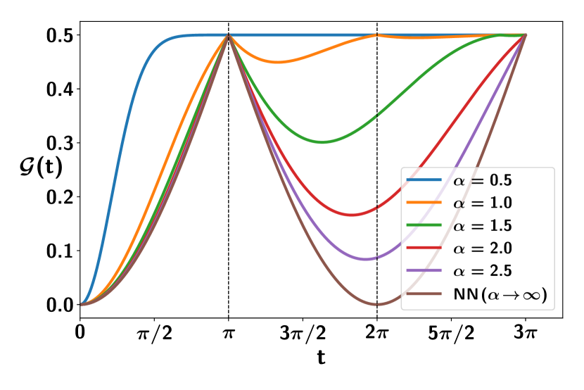
Figure 2: (Color online.) GGM, $\mathcal{G}$ (vertical axis) against time $t$ (horizontal axis) for the $N=5000$-qubit all-to-all connected WGS ($z=N-1$) in $1$D lattice with open boundary condition. Different lines represent different values of decay rate $\alpha$ (from below, $\alpha$ increases). $\mathcal{G}$ reaches maximum value $0.5$ at $t=(2n+1)\pi\forall n\in\mathbb{Z}$ irrespective of $\alpha$ since constant nearest-neighbor interactions is always present in all the situations. Both the axes are dimensionless.

IV Recognizing transition in fall-off rates via GGM of Graph states

To create the weighted graph state with the help of LR Ising Hamiltonian having $z=N-1$, the initial state is taken to be the equal superposition of all the elements in the computational basis, which is a fully separable state having vanishing GGM. Suppose at time $t<0$, there is a strong magnetic field (with respect to the nearest-neighbor interaction strength) in the positive $x$-direction, causing the initial state to be completely polarised in the $\ket{+}$ state Kyaw and Kwek (2018). At $t>0$, sudden quench to the LR Ising Hamiltonian by abruptly turning off the magnetic field also leads to the WGS. The amount of multipartite entanglement generated in the resultant network depends upon the weight of the connection between the vertices, determined by the decay rate of the evolving Hamiltonian and the coordination number.

IV.1 Detection of transition in decaying rate with weighted graph state in 1D

Based on the LR system Hamiltonian and the underlying lattice, the decay rate $\alpha$ possesses various transition points which separates the non-local (strong long-range order) from the quasi-local (weak-long range) order ($\alpha^{*}_{LR}$) and the quasi-local order from the local (short-range) one ($\alpha^{*}_{SR}$) in the ground state of the system. In the quantum spin models, analysis shows that $\alpha^{*}_{LR}=d$, where $d$ is the dimension of the lattice, exhibits the transition from long-range to quasi-local region Koffel et al. (2012); Vodola et al. (2014, 2015); Defenu et al. (2020); Román-Roche et al. (2023); Kaicher et al. (2023).

Let us demonstrate the trends of multipartite entanglement in the WGS constructed from the underlying long range model can capture the transition point in the decay rate $\alpha$.

GGM of the weighted graph state in $1$D. Let us first examine the behavior of GGM of WGS generated via variable-range interaction for different values of $\alpha$ in $1$D (see Fig. 2 in which the behavior of $\mathcal{G}$ with the valuation of time for different $\alpha$ is shown). For any $\alpha$ in the weighted graph states, the maximum value of GGM, $\mathcal{G}=0.5$ is achieved at $t=(2n-1)\pi\forall n\in\mathbb{N}$, since GGM in case of the evolving Hamiltonian with the nearest-neighbor interactions, i.e., $z=1$ is independent of $\alpha$ in Eq. (9) and $\cos\frac{t}{2r^{\alpha}}=0$ $\forall\alpha$ and $r=1$. To detect the transition between non-local and quasi-local/local regimes, we use two identifiers, given by

$$\bar{\mathcal{G}}_{2\pi}(\alpha)=\left.\frac{d\mathcal{G}(\alpha,t)}{dt}\right|_{t=2\pi};\quad\frac{d\mathcal{G}_{2\pi}}{d\alpha}(\alpha)=\frac{d}{d\alpha}\mathcal{G}(\alpha,t=2\pi).$$ (11)

Let us first discuss the extreme points. $\alpha=0$ corresponds to a uniform graph state where each vertex is connected to every other vertex with identical weights Mahto et al. (2022); and $\alpha\to\infty$ leads to a graph state with uniform weights involving with the nearest-neighbor vertices Briegel and Raussendorf (2001); Raussendorf et al. (2003). It becomes the cluster state at $t=\pi,3\pi,5\pi,\ldots$ and GGM of the dynamical state obtained through NN interacting Hamiltonian is oscillatory, with the time period of $2\pi$, i.e., $\mathcal{G}_{2\pi}=0$ and $\bar{\mathcal{G}}_{2\pi}=0$. For any finite $\alpha$, the weights of the all connections contribute, such that these weights decrease polynomially with the increasing distance between vertices ($\phi_{i,i+r}=r^{-\alpha}$). For large $\alpha$, connections other than the nearest neighbors ($\phi_{i,i+1}=1)$ are extremely small and $\mathcal{G}_{2\pi}$ remains close to zero. With the decrease of $\alpha$, the long range connections start to increase. GGM at all times, typically $\mathcal{G}_{2\pi}$is nonvanishing since the absolute product of cosines at $t=2\pi$ in the second term of Eq. (9) keeps on decreasing from unity. On the other hand, at $\alpha=1$, the next-nearest-neighbor makes $\mathcal{G}_{2\pi}=0.5$ since $\cos\frac{2\pi}{4}=0$. When $\alpha$ goes below unity, weights of further distance makes the absolute cosine product almost near zero. This observation serves as a compelling incentive for employing GGM in the identification of $\alpha^{*}_{LR}$ transition point.

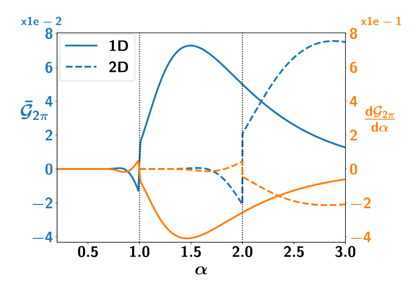
Figure 3: (Color online.) $\bar{\mathcal{G}}_{2\pi}$ (left vertical axis, blue/dark-shaded lines) and $\frac{d\mathcal{G}_{2\pi}}{d\alpha}$ (right vertical axis, orange/light-shaded) as a detector of non-local to quasi-local transition ($\alpha_{LR}^{*}$) against decay rate $\alpha$ (horizontal axis) for $1$D chain (solid lines) and $2$D square lattice (dashed lines). While $\bar{\mathcal{G}}_{2\pi}$ is discontinuous at $\alpha_{LR}^{*}$, $\frac{d\mathcal{G}_{2\pi}}{d\alpha}$ is non-analytic, with the second derivative with respect to $\alpha$ being discontinuous at $\alpha_{LR}^{*}$. The system sizes are $N=5000$ for $1$D chain and $40\times 40$ for $2$D square lattice with $z=N-1$. All axes are dimensionless.

Identifying transitions in falling rate in $1$D. First, notice that $\bar{\mathcal{G}}_{2\pi}$ vanishes until $\alpha\approx 0.7$ and it takes negative value upto $\alpha_{LR}^{*}=1$ while for $\alpha>\alpha_{LR}^{*}$, $\bar{\mathcal{G}}_{2\pi}$ abruptly changes to a positive value and starts increasing as shown in Fig. 3. Secondly, similar discontinuity at $\alpha_{LR}^{*}$ can also be observed from the quantity $\derivative{\mathcal{G}(\alpha,t=2\pi)}{\alpha}=\derivative{\mathcal{G}_{2\pi}}{\alpha}$. Both derivatives of GME of the dynamical state, $\bar{\mathcal{G}}_{2\pi}(\alpha)$ and $\derivative{\mathcal{G}_{2\pi}}{\alpha}$, can successfully identify the transition at $\alpha_{LR}^{*}=1$ from non-local to quasi-local regimes in $1$D by changing its characteristic instantly.

Let us determine whether GME is capable to detect another transition point present $\alpha_{LR}^{*}$. To examine it, we first define the averaged GGM, $\langle\mathcal{G}\rangle_{T}$ with averaging being performed over time, $t=T$ as

$$\langle\mathcal{G}\rangle_{T} = \frac{\int_{0}^{T}\mathcal{G}(t)dt}{T}.$$ (12)

Since $\mathcal{G}$ typically shows some repetitive behavior, with time $T$, the upper limit can be chosen according to such repetitions in $\mathcal{G}$. Extensive numerical simulations indicate that $T=3\pi$ is a good choice as it can capture all the features considered in this work. For $\alpha\rightarrow\infty$ which corresponds to the nearest-neighbor case, we have $\langle\mathcal{G}\rangle_{T=3\pi}\equiv 0.18$ while it reaches its maximum value, $\langle\mathcal{G}\rangle_{T=3\pi}\equiv 0.5$ for $\alpha=0$. In the intermediate $\alpha$, we observe contrasting behavior in $\langle\mathcal{G}\rangle_{T}$ when $0<\alpha<2$, i.e., the evolving Hamiltonian belong to the long-range and quasi-local domains, $\langle\mathcal{G}\rangle$ sharply decreases with the increase of $\alpha$ as shown in Fig. 4, $\langle\mathcal{G}\rangle_{T}$ remains almost constant with $\alpha>>2$, i.e., when the dynamical state arises due to the short range interaction. It indicates that the time-averaged GGM carries signature of the transition point separating long and quasi-local from the short range model.

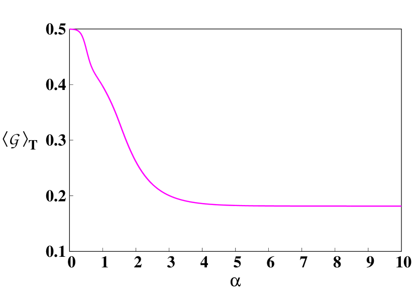
Figure 4: (Color online.) Non- and quasi-local vs. local regimes. The time-averaged value of GGM, $\langle\mathcal{G}\rangle_{T=3\pi}$ (vertical axis) upto time $T=3\pi$ against the interaction parameter, $\alpha$ (horizontal axis). Here $N=10^{6}$-qubit state is generated with coordination number, $z=N-1$ . Starting from maximum value of $\langle\mathcal{G}\rangle_{T=3\pi}=0.5$ at $\alpha=0$ corresponding to end-to-end connected LR system with equal interaction strengths, it decreases drastically until quasi-local region and finally saturates to $\langle\mathcal{G}\rangle_{T=3\pi}\approx 0.18$ for $\alpha\gtrsim 5$, i.e., in the local regime. Both the axes are dimensionless.

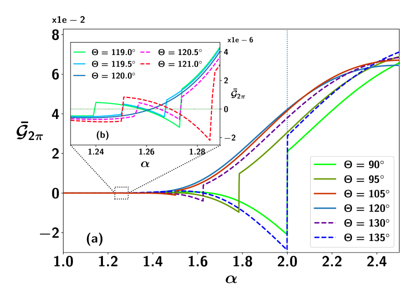
Figure 5: (Color online.) Detection of transition between non-local and quasi-local orders. $\bar{\mathcal{G}}_{2\pi}$ (ordinate) at $\alpha_{LR}^{*}$ with respect to the decay rate $\alpha$ (abscissa) for different $2$D lattice geometries. (a) With increasing distortion angle, $\Theta$ from $90^{\circ}$ (the square lattice), $\alpha_{LR}^{*}$ (the point in which $\bar{\mathcal{G}}_{2\pi}$ shows discontinuity) decreases with $\alpha$ till $\Theta=120^{\circ}$ (the honeycomb lattice). When the distortion angle is increased further, $\alpha_{LR}^{*}$ is now increasing with $\Theta$, and $\alpha_{LR}^{*}=2$ is obtained for $\Theta=135^{\circ}$. (b) Although $\bar{\mathcal{G}}_{2\pi}$ is continuous for the honeycomb lattice, it is still discontinuous when $\Theta$ is close to $120^{\circ}$, which can be used to obtain the transition point for the honeycomb lattice in the asymptotic limit. The system is $N=40\times 40$ in $2$D square lattice with all-to-all connection $(z=N-1)$. All axes are dimensionless.

IV.2 Determining transition in higher dimensional lattices via GGM.

Let us extend the similar analysis of GME acquired by the weighted graph state obtained in two-dimensional lattices. As illustrated in Fig. 1, we begin with a square lattice which is then deformed to other lattice structures with the deformation being given by an angle $\Theta$. Both $\bar{\mathcal{G}}_{2\pi}$ and $\frac{d\mathcal{G}_{2\pi}}{d\alpha}$ exhibit discontinuity at $\alpha_{LR}^{*}=2$, thereby showing their capability to detect the transition point present in a square lattice (see Fig. 5).

Let us concentrate on the other deformed lattices and their transition points which, intuitively, depend on $\Theta$. While the similar behavior of GGM with time is observed in the weighted graph state on these distorted lattices, the transition point of decay rate $\alpha$ changes depending on $\Theta$ as evident from Fig. 5. To make the study quantitatively, we introduce a quantity

$$\Delta\bar{\mathcal{G}}_{2\pi}^{\Theta}=\bar{\mathcal{G}}(\alpha^{*}_{LR}+\delta,t)-\bar{\mathcal{G}}(\alpha^{*}_{LR}-\delta,t),$$ (13)

characterising the jump observed at $\alpha_{LR}^{*}$ for a small increment in $\alpha_{LR}^{*}$, denoted as $\delta$ (which we have taken as $0.001$ for our investigations). As the distortion $\Theta$ is increased (from $90^{\circ}$, in the case of the square lattice), $\alpha_{LR}^{*}$ decreases from $2$ with the discontinuity ($\Delta\mathcal{\bar{G}}_{2\pi}$) being decreased. The trends continue with $\Theta$ till the lattice gets the honeycomb structure, i.e., $\Theta=120^{\circ}$, where $\mathcal{\bar{G}}_{2\pi}$ is continuous ($\Delta\mathcal{\bar{G}}_{2\pi}=0$) as shown in the inset, Fig. 5(b). Specifically, $120^{\circ}>\Theta_{1}>\Theta_{2}>90^{\circ}$, we find $\Delta\mathcal{\bar{G}}_{2\pi}^{\Theta_{1}}<\Delta\mathcal{\bar{G}}_{2\pi}^{\Theta_{2}}$. The limiting case with $\Theta\to 120^{\circ}$ corresponds to the $\alpha$ value ($\bar{\alpha}_{LR}$) where $\mathcal{\bar{G}}_{2\pi}=0$ continuously and changes its sign at $\alpha=\bar{\alpha}_{LR}$. Further, both $\alpha_{LR}^{*}$ and $\Delta\mathcal{\bar{G}}_{2\pi}$ starts increasing, when $\Theta>120^{\circ}$. The transition point, $\alpha_{LR}^{*}=2$, also emerges for the distorted $2$D lattice with $\Theta=135^{\circ}$, but with higher $\Delta\mathcal{\bar{G}}_{2\pi}$ than of $\Theta=90^{\circ}$. The inset (Fig. 5(b)) shows $\Delta\mathcal{\bar{G}}_{2\pi}$ is of the order of $10^{-6}$, which abruptly vanishes for $\Theta=120^{\circ}$. Notice that another discontinuity in $\mathcal{\bar{G}}_{2\pi}$ is observed near $\Theta=120^{\circ}$ which decreases as $\Theta$ is far away from $120^{\circ}$ and the reason behind such observation is not clear from our study.

Summarizing the entire analysis establishes the dependence of $\alpha_{LR}^{*}$ on $\Theta$. In particular, $\alpha_{LR}^{*}$ decreases, when $90^{\circ}<\Theta<120^{\circ}$ while it again increases with $120^{\circ}<\Theta<135^{\circ}$ (see Fig. 6). Notice that $\alpha_{LR}^{*}$ shows a sudden change at $\Theta=120^{\circ}$, although $\mathcal{\bar{G}}_{2\pi}$ is smooth for honeycomb lattice, with the limiting value being $\bar{\alpha}_{LR}^{*}=\alpha_{LR}^{*}(\Theta\to 120^{\circ})=1.261\pm 0.001$. It is worth noticing that when $135^{\circ}<\Theta<150^{\circ}$, $\alpha_{LR}^{*}>2$ although beyond $\Theta>150^{\circ}$, the unit chosen for NN sites is violated. Furthermore, studying the pattern of GME generated with variable-range interaction turns out to be an efficient method for detecting transition points in the fall-off rate.

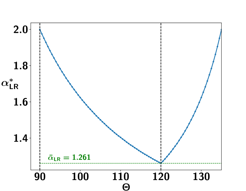
Figure 6: (Color online.) Identifying transitions from non-local to local regime in $2$D lattices. Dependence of the non-local to quasi-local transition point, $\alpha_{LR}^{*}$ (vertical axis) on the distortion angle $\Theta$ (horizontal axis). The transition points in the honeycomb lattice ($\Theta=120^{\circ}$) is obtained asymptotically, where it has the minimum value. Notice that it will be interesting to confirm that the predictions of transitions made by GME of the dynamical states in the deformed square lattices match with the transition points obtained through the correlation length of the ground state. All axes are dimensionless.

IV.3 Replicating time-averaged GGM of an entire lattice with a smaller system size

We now concentrate on the reduction of resource or the depth of the circuit. Specifically we wish to investigate the presence of a critical value concerning the total number of qubits at which the time-averaged multiparty entanglement saturates despite the further augmentation of qubit count. It can be achieved by minimizing the total number of qubits for all-connected weighted graph states with large number of qubits such that its time-averaged GGM is emulated. To address this question mathematically, we define a saturation value in the total number of qubits, denoted as

$$\Delta\langle\mathcal{G}\rangle\equiv\text{min}_{N}|\langle\mathcal{G}(N+1,\alpha)\rangle_{T}-\langle\mathcal{G}(N,\alpha)\rangle_{T}|<\epsilon,$$

for an infinitesimal number $\epsilon$ and the corresponding $N$ represent $N_{sat}$. Here $\epsilon$ is fixed from the accuracy reached in the computation.

Let us illustrate that $N_{sat}$ also carries signature of transition point in $\alpha$. For examination, we fix $\epsilon=10^{-2},10^{-3},5\times 10^{-3},10^{-4}$ with $T=3\pi$. For $1<\alpha\lesssim 2$, the variation of $N_{sat}$ is extremely rapid which is not the case for $\alpha>>2$. For example, with $\epsilon=10^{-4}$ in the LR model with $\alpha=1$, we obtain $N_{sat}=4521$, which decreases drastically to $N_{sat}=29$ for $\alpha=2$. It declines further with the increase of $\alpha$ and $N_{sat}|_{\alpha=3}=9$ and $N_{sat}|_{\alpha=5}=5$ in the local regime. Therefore, $N_{sat}$ becomes single-digit when only short-range interactions are involved in the evolving Hamiltonian while it is moderate in the quasi-local regime and posses a very high value in the LR system.

With the decrease of $\epsilon$, the saturation value $N_{sat}$ grows rapidly in the region $1\lesssim\alpha\lesssim 2$, although beyond this region, the rate of increase is much low, i.e., the value of $N_{sat}$ remains unaltered as shown in Fig. 7 for $\alpha\gtrsim 2$. Let us ask the question – “What is the minimum number of qubits required so that the time-averaged GGM, $\langle\mathcal{G}\rangle_{T=3\pi}$ saturates for a given $\alpha$?” As shown in Fig. 4, with the model having $N=10^{6}$ sites, $\langle\mathcal{G}\rangle_{T=3\pi}=0.331971$ at $\alpha=1.5$. By careful analysis, we find that with $\epsilon=10^{-4}$ and with $N_{sat}=117$ which is the moderate number of qubits, achievable even with current technologies, we can obtain $\langle\mathcal{G}\rangle_{T=3\pi}=0.331961$. However, in the presence of long range interactions, the error has a drastic effect on $\Delta\langle\mathcal{G}\rangle$ and it is nearly impossible to find $N_{sat}<<N$ in this domain.

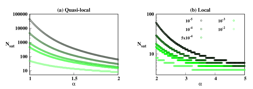
Figure 7: (Color online.) Saturation value of the number of qubits, $N_{sat}$ (ordinate in logarithmic scale) against interaction parameter $\alpha$ (abscissa) for different values of error, $\epsilon$ (mentioned in legends) in the (a) quasi-local and (b) local regions. Here $z=N-1$. Both the axes are dimensionless.

V Mimicking GGM from long-range with short-range model

The emergence of exquisite traits in LR models that are often missing in few body interactive systems has attracted lots of interests. Apart from the physical systems like trapped ions in which long range model arises naturally Häffner et al. (2008), there exist other physical systems including superconducting circuits where one requires two-qubit gates to generate interactions between distant sites Ying et al. (2023); Rasmussen et al. (2021). With the increase of range of interaction, the number of two-qubit gates increases and hence the decoherence effects become prominent. Without compromising the production of GME, our objective is to decrease the range of interactions, i.e., $z$, which can mimic the entanglement properties of LR. Specifically, for a fixed value of $N$, we ask ”what is the minimum coordination number required to produce GGM that can be obtained with fully connected model?” We study the trade off between genuine multiparty entanglement content of a fully connected model and the same created by evolving Hamiltonian with the finite range of interactions.

Let us define the minimum coordination number. For a fixed $N$, and $\alpha$, if the difference of the time-averaged GGM with the variation of $z$ remains constant, we call the minimum $z$ in which $\langle\mathcal{G}\rangle$ saturates as $z_{c}$. Mathematically, we compute

$$\tilde{\Delta}\langle\mathcal{G}\rangle_{z_{c}}\equiv\min_{z}|\langle\mathcal{G}(z=N-1)\rangle_{T}-\langle\mathcal{G}(z)\rangle_{T}|<\epsilon.$$ (15)

with $\epsilon$ being the infinitesimal number which leads to $z_{c}$. Like in the previous case for all values of $\alpha$, we set $T=3\pi$, $\epsilon\approx 10^{-}3$ in the quasi-local and local regions. In the quasi-local and local regions, we observe that it is indeed possible to find $z_{c}$, i.e., there exist $z_{c}$ for a fixed $\alpha$ and $N$, above which $\langle\mathcal{G}\rangle_{T}$ is constant. For example, with $\alpha=1.82$, and $N=120$, the time-averaged GGM obtained with LR model ($z=N-1$) can be attained with $z_{c}=41$. For different $\alpha<2$ values, such $z_{c}$ emerges for a fixed $N$ from $\langle\mathcal{G}\rangle_{3\pi}$ as depicted in Fig. 8. Furthermore, the variation of $z_{c}$ with $\alpha$ can determine the critical point, $\alpha_{SR}^{*}$. Specifically, in the local regime, $z_{c}$ remains almost unaltered with $\alpha$ while its increase is drastic when $1\lesssim\alpha\lesssim 2$ (comparing Figs. 7(a) and 7(b)).

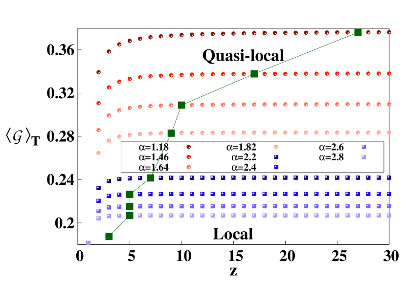
Figure 8: (Color online.) The time-averaged value of GGM, $\langle\mathcal{G}\rangle$ ($y$-axis) upto time $T=3\pi$ for $N=1200$ against coordination number, $z$ (x axis). Different patterns (and colors) indicate quasi-local and local regimes while different shades of a particular color correspond to different values of the interaction parameter $\alpha$. The dark green square boxes suggest the critical value $z=z_{c}$ as in Eq. (15). Here $\epsilon=0.0001$. Notice that the change of $z_{c}$ with the change of $z$ can predict the existence of $\alpha^{*}_{SR}$. Both the axes are dimensionless.

VI Strategy of disconnecting subgraphs in WGS

Let us now move our attention to the effects of single qubit projective measurement on the weighted graph states, thereby disconnecting the part from the entire lattice that is not required for information processing tasks. At the same time, one of our objectives is to design the measurement strategy in such a way that the remaining unmeasured parties share the WGS. Such scheme diminish the qubit count from $N$ to $(N-m)$ while preserving an $(N-m)$-qubit WGS, all the while maintaining the original inter-qubit separation. Fig. 9 illustrates the schematic diagram to achieve the same for $N=5$ and $m=3$ on which the local measurement operators act. Notice that the strategy presented below is valid for both 1D and 2D lattices.

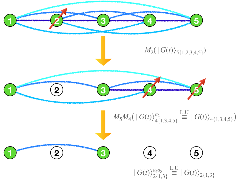
Figure 9: Decoupling scheme of a required circuit via local measurements. Schematic diagram of the protocol for reducing the number of qubits in WGS through local measurements along the $z$-axis. For illustration, let us consider a $5$-party WGS, $\ket{G(t)}_{5\{1,2,3,4,5\}}$. Performing the first measurement $M_{2}$ on the second qubit, the $4$-party state becomes (upto normalization) $M_{2}(\ket{G(t)}_{5\{1,2,3,4,5\}})=\ket{G(t)}^{a_{2}}_{4\{1,3,4,5\}}$ which is local unitarily equivalent to $\text{LU}\ket{G(t)}_{4\{1,3,4,5\}}$. Again performing successive measurements in qubits $4$ and $5$, the two-party output state takes the form $M_{5}M_{4}(\ket{G(t)}_{4\{1,3,4,5\}})=\ket{G(t)}^{a_{5}a_{4}}_{2\{1,3\}}\equiv\text{LU}\ket{G(t)}_{2\{1,3\}}$.

Towards qubit number reduction in WGS. Let us perform a single-qubit projective measurement, $\{M_{k}^{j}|j=1,2\}$ on the qubit $k$ of the $N$-qubit WGS. Therefore, when the outcome $j$ occurs, the normalised output state after tracing out the $k$th qubit can be presented as

$$\ket{\Psi(t)}_{N-1\{12\ldots{(k-1)}{(k+1)}\ldots N\}}^{j_{k}}$$

$$=\frac{M_{k}^{j}\ket{\Psi(t)}_{N\{1\ldots N\}}}{\sqrt{{}_{N\{1\ldots N\}}\bra{\Psi(t)}M_{k}^{j}\ket{\Psi(t)}_{N\{1\ldots N\}}}}.$$ (16)

Theorem 1.

Single qubit measurements in $\sigma_{z}$ basis on $m$ number of qubits situated in arbitrary position on all-to-all connected $N$-qubit weighted graph state provide local unitarily equivalent $(N-m)$-qubit weighted graph state with modified weights where initial qubit position remains fixed.

Proof.

Let us rewrite an $N$-qubit weighted graph state in Eq. (4), following the power law as

$$\ket{G(t)}_{N\{1,2,\ldots,k,\ldots,N\}}$$

$$=\frac{1}{2^{N/2}}\sum_{\eta=0}^{2^{N}-1}\exp\Big(-i\sum_{i=1}^{N-1}\sum_{j>i}^{N}g_{ij}(t)\delta_{a_{i}}^{1}\delta_{a_{j}}^{1}\Big{missing})\ket{\eta},$$ (17)

which consists of all possible states in the computational basis of $N$ qubits with $\ket{\eta}$ being the decimal equivalent of binary values. Performing measurement in the $\sigma_{z}$ basis on the $k$th qubit and selecting the outcome $M^{0}_{k}=\ket{0}_{k}\bra{0}$, the output state takes the form as

$$\ket{G(t)}_{N\{1,2,\ldots,k,\ldots,N\}}^{0_{k}}$$

$$=\frac{1}{2^{N/2}}\sum_{\begin{subarray}{c}r=2\mathbb{Z}\\ r<2^{k}\end{subarray}}\sum_{\eta=r2^{N-k}}^{(1+r)2^{N-k}-1}\exp\Big(-i\sum_{i=1}^{N-1}\sum_{j>i}^{N}g_{ij}(t)\delta_{a_{i}}^{1}\delta_{a_{j}}^{1}\Big{missing})\ket{\eta}.$$

Tracing out the $k$th qubit reduces the binary value of each basis to $(\eta^{\prime}-r2^{N-k})\forall r$ by which we write the corresponding state as

$$\ket{G(t)}_{(N-1)\{1,2,\ldots,k-1,k+1,\ldots,N\}}^{0_{k}}$$

$$=\frac{1}{2^{(N-1)/2}}\sum_{\begin{subarray}{c}r=2\mathbb{Z}\\ r<2^{k}\end{subarray}}\sum_{\eta=r2^{N-k}}^{(1+r)2^{N-k}-1}\exp\Big(-i\sum_{i=1}^{N-1}\sum_{j>i}^{N}g_{ij}(t)\delta_{a_{i}}^{1}\delta_{a_{j}}^{1}\Big{missing})$$

$$\ket{\eta-r2^{N-k}}.$$

(19)

Eventually for each possible value of $\eta$ and $r<2^{k}$, all possible terms in Eq. (19) forms a basis of $(N-1)$-qubit WGS state. Therefore, we can write

$$\ket{G(t)}_{(N-1)\{1,2,\ldots,k-1,k+1,\ldots,N\}}^{0_{k}}$$

$$=\frac{1}{2^{(N-1)/2}}\sum_{\zeta=0}^{2^{N-1}-1}\exp\Big(-i\sum_{\begin{subarray}{c}i=1\\ i\neq k\end{subarray}}^{N-1}\sum_{\begin{subarray}{c}j>i\\ j\neq k\end{subarray}}^{N}g_{ij}(t)\delta_{a_{i}}^{1}\delta_{a_{j}}^{1}\Big{missing})\ket{\zeta}$$

$$=\prod_{\begin{subarray}{c}i=1\\ i\neq k\end{subarray}}^{N-1}\prod_{\begin{subarray}{c}j>i\\ j\neq k\end{subarray}}^{N}U_{ij}\ket{+}_{1}\ket{+}_{2}\otimes\ldots\otimes\ket{+}_{k-1}\ket{+}_{k+1}\otimes\ldots\otimes\ket{+}_{N}$$

$$=\ket{{G}(t)}_{(N-1)\{1,2,\ldots,k-1,k+1,\ldots,N\}},$$

where $\ket{\zeta}\equiv\ket{a_{1}a_{2}\ldots a_{k-1}a_{k+1}\ldots a_{N}}$. Similarly, measuring and tracing out site $l$ on $(N-1)$-qubit WGS state in the computational basis leads to $(N-2)$-qubit WGS state when the outcome is $M_{l}^{0}$ and so on. After $m$ number of such measurements, we obtain $(N-m)$-qubit WGS state, when $M^{0}$ clicks in all the $m$ sites. Specifically, measuring on $k_{1},\ldots,k_{m}$ sites, the resulting state is $(N-m)$-qubit WGS, denoted as $\ket{{G}(t)}^{0_{k_{1}}\ldots 0_{k_{m}}}_{(N-m)\{k\}_{k=1;k\neq k_{1},\ldots,k_{m}}^{N}}\equiv\ket{{G}(t)}_{(N-m)\{k\}_{k=1;k\neq k_{1},\ldots,k_{m}}^{N}}$. The single-site density matrix corresponding to the site $l$ as

$$\rho_{l}^{0}(k_{1},\ldots,k_{m}) = \begin{pmatrix}\frac{1}{2}&x\\ x^{*}&\frac{1}{2}\end{pmatrix}\equiv\rho_{l},$$ (20)

where

$$x=\frac{1}{2^{N-m}}\prod_{\begin{subarray}{c}j=1\\ j\neq l,k_{1},\ldots,k_{m}\end{subarray}}^{N}(1+e^{i\phi_{lj}}),$$ (21)

and $\rho_{l}^{0}(k_{1},\ldots,k_{m})$ denotes the $l$th side density matrix with the measurement outcome on $k_{1},\ldots,k_{m}$ qubits being $M^{0}$.

Let us consider the situation when $M^{1}$ clicks. The single-site density matrix changes to $\rho_{l}^{1}(k_{1},\ldots,k_{m})$ with different off diagonal entries modified by a phase factor as

$$\rho_{l}^{1}(k_{1},\ldots,k_{m})=\begin{pmatrix}\frac{1}{2}&y\\ y^{*}&\frac{1}{2}\end{pmatrix},$$ (22)

where

$$y=\frac{1}{2^{N-m}}e^{i\sum_{r=1}^{m}\phi_{lk_{r}}}\prod_{\begin{subarray}{c}j=1\\ j\neq l,k_{1},\ldots,k_{m}\end{subarray}}^{N}(1+e^{i\phi_{lj}}).$$ (23)

The eigenvalues of $\rho_{l}^{1}(k_{1},\ldots,k_{m})$ and $\rho_{l}^{0}(k_{1},\ldots,k_{m})\equiv\rho_{l}$ are same due to fact that off diagonal entries differ only by a phase factor. Therefore, the output state obtained with the outcome $M^{1}$ is local unitarily connected with the state having $M^{0}$ outcome. Here the local unitary at each site is given by

$$\mathbb{U}_{l}=\begin{pmatrix}e^{i\sum_{r=1}^{m}\phi_{lk_{r}}}&0\\ 0&1\end{pmatrix},$$ (24)

i.e.,

$$\ket{G(t)}^{0_{k_{1}},\ldots,0_{k_{m}}}_{(N-m)\{k\}_{k=1;k\neq k_{1},\ldots,k_{m}}^{N}}$$

$$=\bigotimes_{l\in k}\mathbb{U}_{l}\ket{G(t)}^{1_{k_{1}},\ldots,1_{k_{m}}}_{(N-m)\{k\}_{k=1;k\neq k_{1},\ldots,k_{m}}^{N}}.$$ (25)

Notice that $\mathbb{U}_{l}\in SU(2)$, in general, although for some particular values of $\sum_{r=1}^{m}\phi_{lk_{r}}=2n\pi,(4n+3)\frac{\pi}{2},(4n+1)\frac{\pi}{2}$, the local unitary $\mathbb{U}_{l}$ becomes Clifford unitary Nielsen and Chuang (2010) as it preserves the single-qubit Pauli group. Finally, it is clear that for total $m$ number of measurements on arbitrary qubits, $k_{1},\ldots,k_{m}$, we have to apply local unitary on each qubits depending on the outcome at every step of the measurement except $k_{1},\ldots,k_{m}$, i.e.,

$$\ket{G(t)}_{(N-m)\{k\}_{k=1;k\neq k_{1},\ldots,k_{m}}^{N}}$$

$$=\prod_{j=1}^{m}\bigg{(}\bigotimes_{\begin{subarray}{c}l_{j}=1\\ l_{j}\neq k_{1},\ldots,k_{m}\end{subarray}}^{N}(\delta_{a_{k_{j}}}^{0}\mathbb{I_{l_{j}}}+\delta_{a_{k_{j}}}^{1}\mathbb{U}_{l_{j}})\bigg{)}\ket{G(t)}^{a_{k_{1}},\ldots,a_{k_{m}}}_{(N-m)\{k\}_{k=1;k\neq k_{1},\ldots,k_{m}}^{N}}.$$

∎

Let us illustrate Theorem 1 with an example. For $N=3$, after measuring and tracing out the $2$nd qubit, the output state becomes

$$\ket{G(t)}_{2\{13\}}^{0_{2}}=\frac{1}{2}(\ket{00}+\ket{01}+\ket{10}+e^{-ig_{13}}\ket{11}),$$ (27)

when $\ket{0}$ clicks which is equivalent to $\ket{G(t)}_{2\{13\}}=U_{13}\ket{+}_{1}\ket{+}_{3}$ where the qubits at position $1$ and $3$ are connected. The output state of the outcome, $M^{1}=\ket{1}\bra{1}$ can be written as

$$\ket{G(t)}_{2\{13\}}^{1_{2}} = \frac{1}{2}(\ket{00}+e^{-ig_{23}}\ket{01}+e^{-ig_{12}}\ket{10}$$ (28)

$$+ e^{-i(g_{12}+g_{13}+g_{23})}\ket{11}),$$

which is equivalent to $\ket{G(t)}_{2\{13\}}$ upto local unitary, $\mathbb{U}_{1}\otimes\mathbb{U}_{3}=\text{diag}(e^{i\phi_{21}},1)_{1}\otimes\text{diag}(e^{i\phi_{23}},1)_{3}$. Similarly, starting from $\ket{G(t)}_{5\{12345\}}$, we can generate $\ket{G(t)}_{4\{1345\}}$, $\ket{G(t)}_{3\{135\}}$ and $\ket{G(t)}_{2\{13\}}$ successively by measuring $\sigma_{z}$ on the second, fourth and fifth qubits respectively as shown in Fig. 9.

VII Conclusion

Measurement-based quantum computation (MBQC) is a promising candidate to implement quantum circuits in laboratories and hence it is crucial to identify the ingredient, known as cluster state, which belongs to the set of stabilizer states required for performing MBQC perfectly. They are typically produced by using the nearest-neighbor Ising Hamiltonian from a product state. Instead of nearest-neighbor (NN) interactions, if the product state is evolved with variable-range interactions, weighted graph states possessing exquisite characteristics can be produced, exhibiting some features of the evolving Hamiltonian that NN interactions cannot reveal. We argued the exact expression of generalized geometric measure (GGM) as a function of fall-off rate, range of interactions and time for any system size, in both one- and two-dimensions with varied geometries. It is worth noting that producing GGM for an arbitrary number of sites is computationally demanding since it necessitates calculating the maximum eigenvalues of all possible reduced density matrices and hence with the increase of system size, the computational complexity grows exponentially. In this case, we proved that the maximum eigenvalue obtained only from the single-site reduced density matrix contributes to the GGM. We demonstrated that the time-derivative of GGM in one- and two-dimensions, including lattices formed after deformation from square one, can identify transitions in fall-off rates from long-range to quasi-local regions. On the other hand, we found that the saturation of time-averaged GGM with system size as well as fall-off rates can be employed to predict transitions from quasi-local to local regimes in the evolving Hamiltonian. Furthermore, we observed that, for a certain system size, GGM generated from a finite-range Hamiltonian resembles the behavior of GGM in the long-range models under the quasi-local and local regimes.

We also investigated the effect of measurement along a certain direction on the weighted graph state. We showed that the resultant weighted graph state is local unitarily equivalent to another weighted graph state with fewer qubits, and obtained the relationship between the weights of the pre- and the post-measured states. The present findings demonstrate the potential of WGS as a resource for quantum communication and computation taks.

Appendix A Calculation of reduced density matrices of WGS form PEPS description

Going to the PEPS description Verstraete and Cirac (2004); Dür et al. (2005); Hartmann et al. (2007) of $\ket{\Psi^{\prime}}$ in Eq. (7) based on $G^{\prime}$, each qubit in $B$ is replaced by $n$ virtual qubits (one for each site in $A$), and similarly, each qubit in $A$ is replaced by $N-n$ virtual qubits (one for each site in $B$). The $\ket{\Psi^{\prime}}$ in terms of the virtual qubits can be represented as

$$\ket{\bar{\Psi}^{\prime}}=\bigotimes_{k\in A,l\in B}U_{k,l}\ket{+}_{\bar{k}_{l}}\ket{+}_{\bar{l}_{k}}.$$ (29)

A.1 Action of projection on virtual qubits in $B$

For simplicity, consider $N=3$ with $A=\{1,2\}$ and $B=\{3\}$. Denoting the virtual qubits of $1$ as $\bar{1}_{3}$, of $2$ as $\bar{2}_{3}$ and of $3$ as $\bar{3}_{1}$ and $\bar{3}_{2}$, in the PEPS form, the state is

$$\ket{\bar{\Psi}^{\prime}}_{N=3} = \left(U_{13}\ket{+}_{\bar{1}_{3}}\ket{+}_{\bar{3}_{1}}\right)\left(U_{23}\ket{+}_{\bar{2}_{3}}\ket{+}_{\bar{3}_{2}}\right)$$

$$= \ket{+}_{\bar{1}_{3}}\ket{+}_{\bar{2}_{3}}\ket{0}_{\bar{3}_{1}}\ket{0}_{\bar{3}_{2}}+\ket{\zeta_{1}}_{\bar{1}_{3}}\ket{\zeta_{2}}_{\bar{2}_{3}}\ket{1}_{\bar{3}_{1}}\ket{1}_{\bar{3}_{2}}+\dots$$

with $\ket{\zeta_{k}}_{\bar{k}_{3}}=(\ket{0}_{\bar{k}_{3}}+e^{-ig_{k3}}\ket{1}_{\bar{k}_{3}})/\sqrt{2}$ for $k=1,2$ and only the terms surviving in the projections are shown after the action of unitaries. After projection from virtual to physical qubit in position $3$, we get

$$P_{3}\ket{\bar{\Psi}^{\prime}}_{N=3} = \Big{(}\ket{0_{3}}\bra{0_{\bar{3}_{1}}0_{\bar{3}_{2}}}+\ket{1_{3}}\bra{1_{\bar{3}_{1}}1_{\bar{3}_{2}}}\Big{)}\ket{\bar{\Psi}^{\prime}}_{N=3}$$

$$= \ket{++}_{\bar{1}_{3}\bar{2}_{3}}\ket{0}_{3}+\ket{\zeta_{1}\zeta_{2}}_{\bar{1}_{3}\bar{2}_{3}}\ket{1}_{3}$$

$$= U_{13}U_{23}\ket{+}_{\bar{1}_{3}}\ket{+}_{\bar{2}_{3}}\ket{+}_{3},$$

which is not normalized. Therefore, for $N$-qubit state, the action of projections $P_{l}$ on qubits in B gives a state (upto normalization) of the form $\ket{\Psi^{P}}=\bigotimes\limits_{l\in B}\left[\prod_{k\in A}U_{kl}\ket{+}_{\bar{k}_{l}}\ket{+}_{l}\right]$ that is a tensor product of $N-n$ states. This allows us to individually trace out each qubit in B.

A.2 Partial trace over $B$

Let us consider again $N=3$ case with $A=\{1\}$ (virtual qubits $\bar{1}_{2},\bar{1}_{3}$) and $B=\{2,3\}$. Then from the previous discussion, $\ket{\Psi^{P}}=\Big{(}U_{12}\ket{+}_{\bar{1}_{2}}\ket{+}_{2}\Big{)}\bigotimes\Big{(}U_{13}\ket{+}_{\bar{1}_{3}}\ket{+}_{3}\Big{)}$ and the partial trace over $\{2,3\}$ can be done independently, by which we obtain $\bar{\rho}_{1}=\bar{\rho}_{1}(2)\bigotimes\bar{\rho}_{1}(3)$, where $\bar{\rho}_{1}(l)=\ket{+}_{\bar{1}_{l}}\bra{+}+\ket{\zeta_{l}}_{\bar{1}_{l}}\bra{\zeta_{l}}$, with $\ket{\zeta_{l}}_{\bar{1}_{l}}=(\ket{0}_{\bar{1}_{l}}+e^{-ig_{1l}}\ket{1}_{\bar{1}_{l}})/\sqrt{2}$ for $l=1,2$.

It is important to note that although not normalized, each $\bar{\rho}_{1}(l)$ is a positive semi-definite matrix with all diagonal values as $1$. Generalizing this effect to $N$-qubit WGS, with bipartition $A$ of $n$ sites, the reduced density matrix is

$$\bar{\rho}_{A}=\bigotimes_{l\in B}\bar{\rho}_{A}(l)=\bigotimes_{l\in B}2^{n-1}\Big{(}\ket{+}_{\bar{1}_{l}\bar{2}_{l}\dots\bar{n}_{l}}\bra{+}+\ket{\zeta_{l}}_{\bar{1}_{l}\bar{2}_{l}\dots\bar{n}_{l}}\bra{\zeta_{l}}\Big{)},$$ (30)

where $\ket{\zeta_{l}}_{\bar{1}_{l}\bar{2}_{l}\dots\bar{n}_{l}}=(\ket{0}_{\bar{1}_{l}\bar{2}_{l}\dots\bar{n}_{l}}+\left(\prod\limits_{k\in A}e^{-ig_{kl}}\right)\ket{1}_{\bar{1}_{l}\bar{2}_{l}\dots\bar{n}_{l}})/\sqrt{2}$ for $l\in B$ and each $\bar{\rho}_{A}(l)$ is a $2^{n}\times 2^{n}$ positive semi-definite matrix, scaled by $2^{n-1}$ so that all the diagonal values of each $\bar{\rho}_{A}(l)$ is unity. Note that the weights are encoded in the off-diagonal terms as phases. Proper normalization of $\bar{\rho}_{A}$ is done only at the end after the projection on virtual qubits in $A$.

A.3 Action of projection on virtual qubits in $A$

For the above case of $N=3$ with $A=\{1\}$ (virtual qubits $\bar{1}_{2},\bar{1}_{3}$) and $B=\{2,3\}$, $\bar{\rho}_{1}(l)=\ket{0}_{\bar{1}_{l}}\bra{0}+x_{1l}\ket{1}_{\bar{1}_{l}}\bra{0}+x^{*}_{1l}\ket{0}_{\bar{1}_{l}}\bra{1}+\ket{1}_{\bar{1}_{l}}\bra{1}$, where $x_{1l}=\frac{1+e^{-ig_{1l}}}{2}$ for $l=2,3$. From the form of the inevitable projection $P_{k}$ for $k\in A$, the only terms in the tensor product of virtual qubits that will contribute are ones formed only via $\ket{00}_{\bar{1}_{2}\bar{1}_{3}},\ket{11}_{\bar{1}_{2}\bar{1}_{3}}$ and their dual vectors. After applying $P_{k}$, we finally get

$$\rho^{\prime}_{1}=\begin{pmatrix}1&x_{12}x_{13}\\ x^{*}_{12}x^{*}_{13}&1\end{pmatrix}=\bar{\rho}(2)\ostar\bar{\rho}(3),$$ (31)

where $\ostar$ is the Hadamard product. This can be generalized for $A$ with $n$ sites, as $\rho^{\prime}_{A}=\underset{l\in B}{\ostar}\bar{\rho}_{A}(l)$, where $\bar{\rho}_{A}(l)$ is represented as in Eq. (30) scaled all diagonal entries to unity.