A theoretical framework for learning through structural plasticity

Abstract

A growing body of research indicates that structural plasticity mechanisms are crucial for learning and memory consolidation. Starting from a simple phenomenological model, we exploit a mean-field approach to develop a theoretical framework of learning through this kind of plasticity, capable of taking into account several features of the connectivity and pattern of activity of biological neural networks, including probability distributions of neuron firing rates, selectivity of the responses of single neurons to multiple stimuli, probabilistic connection rules and noisy stimuli. More importantly, it describes the effects of consolidation, pruning and reorganization of synaptic connections. This framework will be used to compute the values of some relevant quantities used to characterize the learning and memory capabilities of the neuronal network in a training and validation procedure as the number of training patterns and other model parameters vary. The results will then be compared with those obtained through simulations with firing-rate-based neuronal network models.

I Introduction

Together with temporary and reversible changes of synaptic efficacy such as short and long-term plasticity mechanisms, structural changes in the synaptic morphology of the network are fundamental mechanisms that take place in healthy brains. These changes occurs at longer time scales than the short or long-term mechanisms mentioned above, and consist in the consolidation, creation of new synapses or erasure of synapses that have not been consolidated. This type of synaptic plasticity, which is called structural plasticity, can be spontaneous, but also experience-based [5], and it has a key role in the stabilization of new concepts that has to be kept in memory after learning [12].
Indeed, it is known that neurotransmitters can be neurotrophic factors, i.e. participate in growth or suppression of dendritic spines, synapses, axon and dendrites [26, 23, 33]. Thus, structural plasticity is a neural-activity-driven mechanism, which can increase or decrease the number of synapses. Such modifications are then flanked by an homeostatic kind of structural plasticity, which has a balancing effect achieved with adding or removing synapses, as described in [11].
Moreover, the number of synapses in the brain can change over time. In [20] it is shown that synaptic density reaches the highest values at $1$-$2$ years age, it drops during adolescence and stabilizes between age $16$-$72$, followed by a slight decline. However, although synaptic density remains approximately stable during adulthood, rewiring of network connections occurs as well in order to efficiently store new memories. The increase of connections in high activity regions (and vice versa), together with the rearrangement of synapses leads to a fine-tuning of the brain’s circuits [36], because on one hand some synapses can be strengthened through long-term potentiation (LTP) and new connections can be formed next to the already potentiated ones to further enhance synaptic transmission, on the other hand when the presynaptic and postsynaptic neuron activities have low correlation their connection are likely to be removed. The latter process is called synaptic pruning and it is considered essential for optimizing activity propagation and memory capacity[9, 21, 22]. Furthermore, it is commonly believed that synaptic pruning and rewiring dysfunction are one of the neural correlate of developmental disorders such as autism or schizophrenia [3, 28], leading to, respectively, an higher or lower synaptic density with respect to neurotypical subjects[19, 30, 14].
In the last decades computational neuroscience has investigated brain dynamics at different scales, from cellular [25] to mesoscopic and macroscopic through mean-field approaches [45, 1, 18, 32, 24, 37, 7, 8]. Regarding synaptic plasticity, computational models were mostly focused on plasticity mechanisms that involve strengthening or weakening of existing synapses, like short-term plasticity (STP) [43] or spike timing-dependent plasticity (STDP) [17] and on their role in short-term, long-term, working memory and learning [27, 42, 39, 2, 15, 6]. Only in recent times computational models of structural plasticity and connectivity rearrangements during learning were developed, showing intriguing results. [21] and [22] describe a model of structural plasticity based on ”effectual connectivity”, defined in these works as the fraction of synapses able to represent a memory stored in a network. By structural plasticity, effectual connectivity is improved, since synapses that do not code for the memory are moved in order to optimize network’s connectivity. Their model defines synapses using a Markov model of three states: potential (i.e. not instantiated), instantiated but silent or instantiated and consolidated. Structural plasticity is thus related to the passage of the synapses from a potential state to an instantiated state (and vice versa), whereas changes only related to the synaptic weight are described by the consolidation of the instantiated synapses. With such a model, it is possible to show that networks with structural plasticity have higher or comparable memory capacity to networks with dense connectivity and it is possible to explain some cognitive mechanism such as the spacing effect [21].
[40] simulated a spiking neural network with structural plasticity and STDP, showing that structural plasticity reduces the amount of noise of the network after a learning process, thus making the network able to have a clearer output. Furthermore, such a network with structural plasticity shows higher learning speed than the same network with only STDP implemented.
Some new insights about the importance of synaptic pruning are also shown in [29], in which different pruning rates were studied suggesting that a slowly decreasing rate of pruning over time leads to more efficient network architectures.
As discussed above, the biochemical and biophysical mechanisms underlying structural plasticity are extremely complex and only partially understood to date. For this reason, rather than attempting to build a biologically detailed model, this work exploits a relatively simple phenomenological model, including both the activity-driven and the homeostatic contributions; despite the lower complexity, this model accounts for the effects of structural plasticity in terms of the consolidation of synaptic connections between neurons with a high activity correlation as well as those of pruning and rewiring the connections for which this correlation is lower. This approach is also justified by the requirement for a simple and effective computational model suitable for simulating networks with a relatively large number of neurons and connections and for representing learning processes with sizable numbers of training and validation patterns. This model will then serve as the foundation for the creation of a mean-field-based theoretical framework for learning through synaptic plasticity capable of accounting for a variety of biological network properties. This framework will be used in a training and validation procedure to characterize learning and memory capacity of plastic neuronal networks as the number of training patterns and other model parameters vary. The results will then be compared with those obtained through simulations based on firing-rate-based neuronal networks. The model considers two populations of neurons, $\mathcal{P}_{1}$ and $\mathcal{P}_{2}$, with synaptic connections directed from the first to the second population. During the training phase, $\mathcal{P}_{1}$ receives an input stimulus, while $\mathcal{P}_{2}$ receives a contextual stimulus. The model assumes that synaptic consolidation is a probabilistic process driven by pre- and postsynaptic spiking activity. For each pattern given in input to the model, only a small fraction of neurons contribute to this process. Connection consolidation is complemented by a rewiring process: connection pruning, which eliminates unconsolidated connections, and creation of new connections, which restores network balance. This framework does not specifically refer to a particular region of the brain; rather, it is built on characteristics that are ubiquitous for several brain areas.
The proposed approach is capable of accounting for different probabilistic connection rules, firing rate probability distributions, presence of noise in stimuli, thus providing a general framework to study the impact of structural plasticity in learning on large-scale neuronal network models.

II Materials and Methods

Here we introduce the theoretical framework for the structural plasticity model and the firing-rate-based network model used to validate it and estimate its learning capability. Firstly, we present the general model of two neuron populations, and secondly the theoretical framework is divided into two possible approaches: a simple, discrete rate model in which neurons can only assume two possible firing rates values and a more realistic continuous rate model in which firing rates follow a continuous probability distribution. Finally, we introduce the computational simulation framework.

II.1 Two neuron populations model

The neuronal network model used in this work consists of two neuron populations, $\mathcal{P}_{1}$ and $\mathcal{P}_{2}$, consisting of $10^{5}$ neurons each. This number corresponds roughly to the number of neurons in $1\text{ mm}^{2}$ of cerebral cortex. The exchange of information between the two populations takes place through the connections from the population $\mathcal{P}_{1}$ to the population $\mathcal{P}_{2}$, which in the model are on average $5\cdot 10^{3}$ per neuron of $\mathcal{P}_{2}$, for a total of $5\cdot 10^{8}$ connections. Each connection has an initial synaptic weight of $\mathcal{W}_{\text{b}}$. The first population ($\mathcal{P}_{1}$) receives an input stimulus (e.g., visual) mimicked by the activation of the neurons with a firing rate pattern associated to it. During the training stage, in addition to the signal from $\mathcal{P}_{1}$, the second population receives another stimulus (e.g., auditory), that we identify as a contextual stimulus. Figure 1 depicts a simple scheme of the network. Structural plasticity is modelled following the categories proposed by [11], i.e., activity-dependent and homeostatic. The firing rate patterns of the two populations have a role in the activity-dependent structural plasticity. The consolidation of a synaptic connection occurs when the firing rates of both the presynaptic and the postsynaptic neurons are concurrently above a certain threshold (the definition of which will vary depending on the model). The synaptic weight of a consolidated connection increases from $\mathcal{W}_{\text{b}}$ to a value $\mathcal{W}_{\text{c}}>\mathcal{W}_{\text{b}}$. Once a synaptic connection has been consolidated, it will maintain the synaptic weight $\mathcal{W}_{\text{c}}$, without the possibility of returning to the initial state $\mathcal{W}_{\text{b}}$. This approach is a computationally-effective way of representing the biological structural changes that make a consolidated connection strong and durable. The sets of input and contextual patterns used for network training are independent firing-rate patterns of the two populations randomly generated from predefined firing rate probability distributions, which can be either discrete or continuous. The training process is performed using $\mathcal{T}$ independent input patterns, together with the corresponding contextual stimuli. A diagram of the training and validation processes is shown in Figure 1. During training, when both input and contextual stimulus are used, a fraction of the neurons in the population $\mathcal{P}_{2}$ will assume a rate above threshold. These neurons, called coding, or selective neurons, play a vital role in input coding. The existence of neurons showing selective firing rate in response to specific stimuli is largely confirmed by experimental results. The average input signal to these neurons will be called $\langle\mathcal{S}_{\text{2}}\rangle$. The non-selective neurons of $\mathcal{P}_{2}$ will instead be called non-coding or background neurons, and their average input signal will be indicated with $\langle\mathcal{S}_{\text{b}}\rangle$. The proposed model accounts for the ability of the network to learn the association between input patterns and the corresponding contextual stimuli.

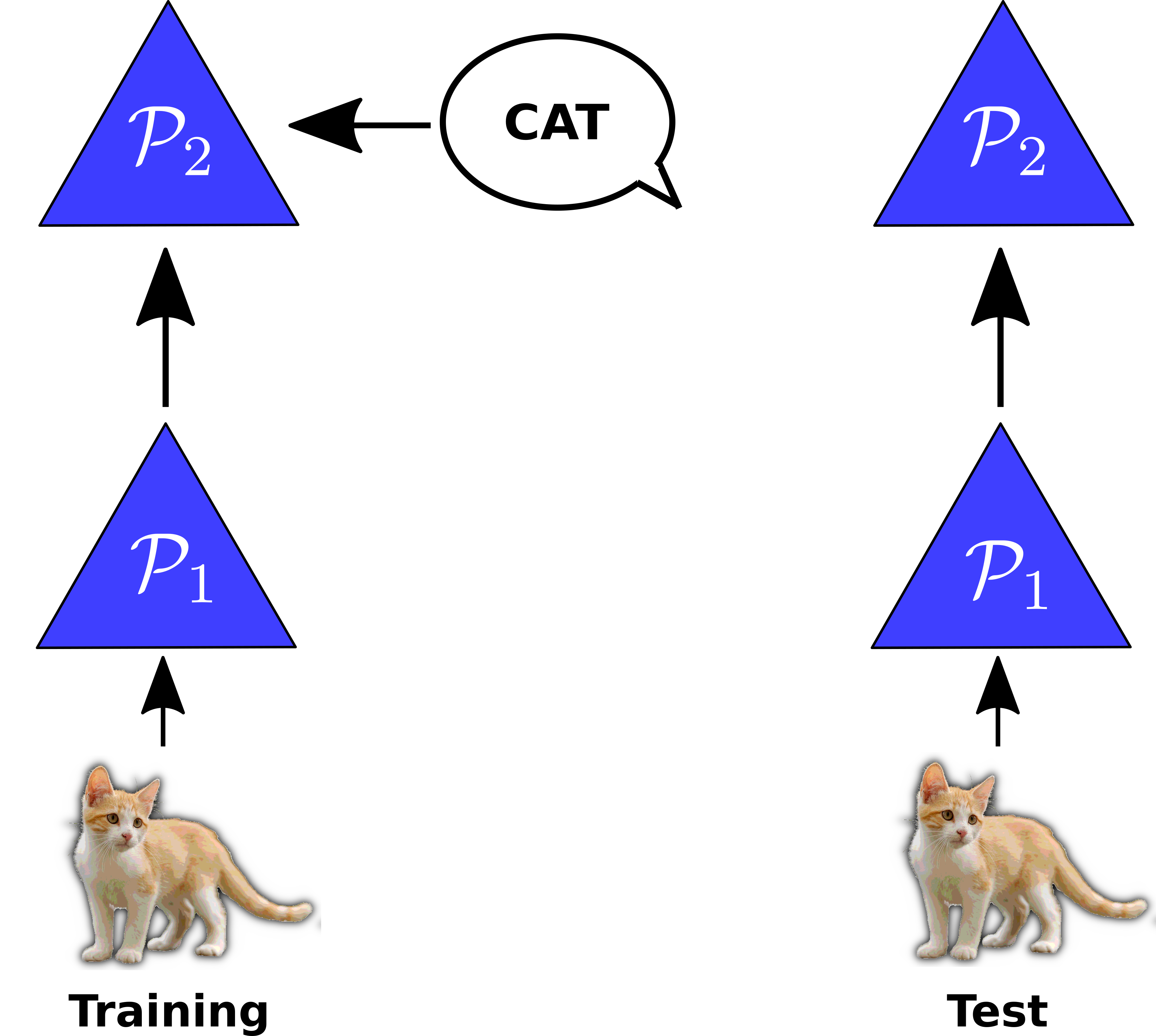
Figure 1: Schematic representation of the network model through a block diagram. During training (left), a visual stimulus is injected into $\mathcal{P}_{1}$ and an auditory stimulus is injected into $\mathcal{P}_{2}$ as contextual stimulus. In test phase (right) one of the visual patterns is injected without the corresponding contextual stimulus. The cat image is adapted from Golden tabby and white kitten by Marie-Lan Nguyen / Wikimedia Commons / CC-BY 2.5.

We may distinguish two different types of models based on the potential values that the neuron firing rate can assume:

• Discrete model the rates of the neurons can assume only two discrete values $\nu_{\ell}$ (low rate) and $\nu_{\text{h}}$ (high rate);

• Continuous model the rate of neurons can assume values from a continuous probability distribution.

In this work, in agreement with the experimental observations, a log-normal distribution of the firing rate has been used for the continuous model [35]. In the next section we will derive the mean-field equations for these two models, which are summarized in the following tables.

Summary
Populations	$\mathcal{P}_{1}$, $\mathcal{P}_{2}$
Connectivity	sparse random connectivity
Neurons	firing-rate-based models of point-like neurons
Synapses	structural plasticity
Input	firing rate pattern extracted from a discrete or continuous probability distribution

Populations
Name	Elements	Size
$\mathcal{P}_{1}$	point-like neurons	$\mathcal{N}_{1}$
$\mathcal{P}_{2}$	point-like neurons	$\mathcal{N}_{2}$

Table 1: Description of the network model (continued on next page).

Neuron
Type	firing-rate-based neuron model
Firing rate distribution	• discrete model: the firing rates can assume only two discrete values $\nu_{\text{h}}$ (high rate) and $\nu_{\ell}$ (low rate); • continuous model: the firing rates can assume values from a continuous probability distribution; this work uses a lognormal distribution

Connectivity
Source	Target	Pattern
$\mathcal{P}_{1}$	$\mathcal{P}_{2}$	• random, independent; in-degrees (i.e., incoming connections) can be homogeneous, with a fixed number of $\mathcal{C}$ connections per neuron of $\mathcal{P}_{2}$, or driven by a Poisson distribution; • synaptic weights are $\mathcal{W}_{\text{b}}$ for unconsolidated connections and $\mathcal{W}_{\text{c}}$ for consolidated ones, with $\mathcal{W}_{\text{c}}>\mathcal{W}_{\text{b}}$; • multiple connections between the same couple of presinaptic and postsinaptic neurons (“multapses”) are allowed by default, but they can be disabled.

Synapse
Type	structural plasticity
Description	initial synaptic weight are set to $\mathcal{W}_{\text{b}}$ for all the instantiated connections; when a training pattern is used, considering a connection between a $\mathcal{P}_{1}$ neuron $i$ and a $\mathcal{P}_{2}$ neuron $j$: • (discrete model) $\mathcal{W}_{\text{b}}\rightarrow\mathcal{W}_{\text{c}}$ if $\nu_{\text{i}}=\nu_{\text{j}}=\nu_{\text{h}}$ • (continuous model) $\mathcal{W}_{\text{b}}\rightarrow\mathcal{W}_{\text{c}}$ if $\nu_{\text{i}}>\nu_{\text{t,1}}$ and $\nu_{\text{j}}>\nu_{\text{t,2}}$ Once a connection is consolidated, it cannot return to the initial weight.

Connection rewiring

Description

periodically, unconsolidated connections are pruned, and new connections are created: if $h$ is the number of consolidated incoming connections of a neuron of $\mathcal{P}_{2}$, $\mathcal{C}-h$ new connections will be created, were $\mathcal{C}$ is a fixed number if the fixed-indegree connection rule is used, while it is extracted from a Poisson distribution if the Poisson-indegree rule is selected; in both cases, the presynaptic neurons are randomly extracted from $\mathcal{P}_{1}$.

Input stimulus
Description	firing rate pattern of the neurons of $\mathcal{P}_{1}$ selected from the training or from the test set.

Contextual stimulus
Description	firing rate pattern of the neurons of $\mathcal{P}_{2}$ selected from the training set; used only in the training phase.

Table 1: Description of the network model (continued on next page).

Train set
Type	set of $T$ independent firing-rate patterns of the neurons of $\mathcal{P}_{1}$ (input stimulus) and $\mathcal{P}_{2}$ (contextual stimulus)
Description	each pattern is randomly generated from predefined firing rate probability distributions, which can be either discrete or continuous: • discrete model: the firing rates can assume only two discrete values $\nu_{\text{h}}$ (high rate) and $\nu_{\ell}$ (low rate) with probabilities $p_{1}$ and $q_{1}=1-p_{1}$ in the $\mathcal{P}_{1}$ population, $p_{2}$ and $q_{2}=1-p_{2}$ in the $\mathcal{P}_{2}$ population. • continuous model: the firing rates can assume values on the basis of a continuous probability distribution; this work uses a lognormal distribution.

Test set
Type	set of $V$ firing-rate patterns of the neurons of $\mathcal{P}_{1}$ (input stimulus)
Description	each pattern is randomly extracted from the train set and eventually altered by adding noise from a predefined distribution: • discrete model: the pattern is left unchanged; • continuous model: the firing rate of each neuron is modified by adding a random deviation extracted from a predefined probability distribution; in this work we used a truncated Gaussian distribution.

Table 1: Description of the network model (continued).

Network and connectivity
Name	Value	Description
$\mathcal{N}_{1}$	$100000$	number of neurons of $\mathcal{P}_{1}$
$\mathcal{N}_{2}$	$100000$	number of neurons of $\mathcal{P}_{2}$
$\mathcal{C}$	$5000$	number of connection in-degrees per neuron of $\mathcal{P}_{2}$
$\mathcal{T}$	variable	number of training patterns
$s$	100	connection rewiring step

Neuron
Name	Value	Description
$\nu_{\ell}$	$2.0\,\text{spikes/s}$	low firing rate
$\nu_{\text{h}}$	$50\,\text{spikes/s}$	high firing rate

Synapse
Name	Value	Description
$\mathcal{W}_{\text{b}}$	$0.1$ pA	baseline synaptic weight
$\mathcal{W}_{\text{c}}$	$1$ pA	consolidated synaptic weight

Stimulus
Name	Value	Description
$p_{1}$	$0.001$	probability for a neuron of $\mathcal{P}_{1}$ of having high rate when an input stimulus is injected
$p_{2}$	$0.001$	probability for a neuron of $\mathcal{P}_{2}$ of having high rate when a contextual stimulus is injected

Table 2: Model parameters.

II.1.1 Discrete rate model

As previously mentioned, in this model the input and contextual stimuli are represented by discrete firing-rate patterns of the two populations, $\mathcal{P}_{1}$ and $\mathcal{P}_{2}$ respectively, in which the firing rate of each neuron can assume only two possible values, $\nu_{\text{h}}$ (high rate) or $\nu_{\ell}$ (low rate). Each training example consists of two patterns, one representing the input stimulus to the population $\mathcal{P}_{1}$, the other representing the contextual stimulus to the population $\mathcal{P}_{2}$. The pattern representing the input stimulus is generated by randomly extracting the firing rate of each neuron of $\mathcal{P}_{1}$ from the two values, $\nu_{\text{h}}$ and $\nu_{\ell}$, with probabilities $p_{1}$ and $q_{1}=1–p_{1}$, respectively. The corresponding pattern for the contextual stimulus is generated in a similar way, extracting the values of the firing rates of the $\mathcal{P}_{2}$ neurons, $\nu_{\text{h}}$ or $\nu_{\ell}$, with probabilities $p_{2}$ and $q_{2}=1–p_{2}$, respectively. The mean number of high-rate neurons in the two populations will be:

$$\begin{split}N_{h,1}&=\mathcal{N}_{1}p_{1}\\ N_{h,2}&=\mathcal{N}_{2}p_{2}\end{split}$$ (1)

where $\mathcal{N}_{1}$ and $\mathcal{N}_{2}$ indicate the number of neurons of $\mathcal{P}_{1}$ and $\mathcal{P}_{2}$, respectively. A connection will be consolidated in a training example if both the presynaptic and the postsynaptic neuron assume a high firing rate $\nu_{\text{h}}$. The probability that a generic connection is consolidated in a single example is $p_{1}p_{2}$, and thus the probability that it is not consolidated after $\mathcal{T}$ training examples is $(1-p_{1}p_{2})^{\mathcal{T}}$. The probability $p$ that a connection is consolidated in at least one of the $\mathcal{T}$ training examples is given by the complement of the previous expression:

$$p=1-(1-p_{1}p_{2})^{\mathcal{T}}$$ (2)

The product of this expression by the number of incoming connections per neuron $\mathcal{C}$ gives us the average number of consolidated connections per neuron:

$$\langle k\rangle=\mathcal{C}\Bigl{[}1-(1-p_{1}p_{2})^{\mathcal{T}}\Bigr{]}=\mathcal{C}p$$ (3)

For each neuron we will therefore have on average $\langle k\rangle$ consolidated connections with synaptic weight $\mathcal{W}_{\text{c}}$ and $\mathcal{C}-\langle k\rangle$ unconsolidated connections with synaptic weight $\mathcal{W}_{\text{b}}$.

The test set consists of $V$ firing-rate patterns of the neurons of $\mathcal{P}_{1}$, randomly extracted from the $\mathcal{T}$ input patterns of the train set. In the discrete rate model, the pattern are unaltered, thus each input patter of the test set is identical to an input pattern of the train set. The contextual stimuli are not used in the validation phase.

The average rate of the neurons in the population $\mathcal{P}_{1}$ is

$$\langle\nu\rangle=p_{1}\nu_{\text{h}}+(1-p_{1})\nu_{\ell}$$ (4)

The input signal targeting a non-coding neuron of $\mathcal{P}_{2}$ (i.e., a background neuron) is equal to the weighted sum of the signals coming from the $\mathcal{C}$ connections:

$$\mathcal{S}_{\text{b}}=\mathcal{W}_{\text{c}}\sum_{i=1}^{k}\nu_{i}+\mathcal{W}_{\text{b}}\sum_{i=1}^{\mathcal{C}-k}\xi_{i}$$ (5)

where $\mathcal{C}$ is the number of incoming connections, $k$ is the number of consolidated connections, $\nu_{i}$ are the firing rates of the neurons connected to the consolidated connections and $\xi_{i}$ are the firing rates of the neurons connected to the unconsolidated connections. From the linearity of $\mathcal{S}_{\text{b}}$ with respect to $\nu_{i}$ and $\xi_{i}$ and from the fact that the rates of presynaptic neurons have the same mean value $\langle\nu\rangle$, it follows that

$$\langle\mathcal{S}_{\text{b}}\rangle=[\mathcal{W}_{\text{c}}\langle k\rangle+\mathcal{W}_{\text{b}}(\mathcal{C}-\langle k\rangle)]\langle\nu\rangle$$ (6)

In this equation, we can clearly observe two distinct contributions: one related to consolidated connections, which depends on the mean value $\langle k\rangle$, and the other related to unconsolidated connections, which depends on $\mathcal{C}-\langle k\rangle$. From this result we can now calculate the variance on the background signal, which is defined as:

$$\sigma_{b}^{2}=\langle(\mathcal{S}_{\text{b}}-\langle\mathcal{S}_{\text{b}}\rangle)^{2}\rangle$$ (7)

Using Equations 5 and 6, we can compute the variance as:

$$\sigma_{b}^{2}=\langle\Bigl{[}\mathcal{W}_{\text{c}}\sum_{i=1}^{k}\nu_{i}+\mathcal{W}_{\text{b}}\sum_{i=1}^{\mathcal{C}-k}\xi_{i}-[\mathcal{W}_{\text{c}}\langle k\rangle+\mathcal{W}_{\text{b}}(\mathcal{C}-\langle k\rangle)]\langle\nu\rangle\Bigr{]}^{2}\rangle$$ (8)

Taking advantage of the equality $\langle k\rangle=k+(\langle k\rangle-k)$, we can rewrite:

$$\mathcal{W}_{\text{c}}\langle k\rangle+\mathcal{W}_{\text{b}}(\mathcal{C}-\langle k\rangle)=\mathcal{W}_{\text{c}}k+\mathcal{W}_{\text{c}}(\langle k\rangle-k)+\mathcal{W}_{\text{b}}\Bigl{[}(\mathcal{C}-k)+(k-\langle k\rangle)\Bigr{]}=$$ (9)

$$=\mathcal{W}_{\text{c}}k+\mathcal{W}_{\text{b}}(\mathcal{C}-k)+\mathcal{W}_{\text{c}}(\langle k\rangle-k)+\mathcal{W}_{\text{b}}(k-\langle k\rangle)$$

Inserting this last expression in Equation 8 and rewriting the terms with the multiplicative factors $k$ and $\mathcal{C}-k$ with summations, such as for example $\mathcal{W}_{\text{c}}k\langle\nu\rangle=\mathcal{W}_{\text{c}}\sum_{i=1}^{k}\langle\nu\rangle$, we obtain:

$$\sigma_{b}^{2}=\langle\Bigl{[}\mathcal{W}_{\text{c}}\sum_{i=1}^{k}(\nu_{i}-\langle\nu\rangle)+\mathcal{W}_{\text{b}}\sum_{i=1}^{\mathcal{C}-k}(\xi_{i}-\langle\nu\rangle)+(k-\langle k\rangle)(\mathcal{W}_{\text{c}}-\mathcal{W}_{\text{b}})\langle\nu\rangle\Bigr{]}^{2}\rangle$$ (10)

Taking into account that the mixed terms go to zero since $\sum_{i}\langle(x_{i}-\langle x\rangle)\rangle=0$, setting $\sum_{i}(x_{i}-\langle x\rangle)^{2}=\sigma^{2}_{x}$, we will have that:

$$\sigma_{b}^{2}=\Bigl{[}\mathcal{W}_{\text{c}}^{2}\langle k\rangle+\mathcal{W}_{\text{b}}^{2}(\mathcal{C}-\langle k\rangle)\Bigr{]}\sigma_{\nu}^{2}+(\mathcal{W}_{\text{c}}-\mathcal{W}_{\text{b}})^{2}\sigma_{k}^{2}\langle\nu\rangle^{2}$$ (11)

where $\sigma_{k}^{2}=\langle(k-\langle k\rangle)^{2}\rangle$. In the previous formula we note two contributions depending respectively on the variance of the firing rate and on the variance of the number of consolidated connections. The value of the variance of $k$ is not shown here, but is derived in Appendix B, whereas the variance of the rate is, by definition, $\sigma^{2}_{\nu}=\langle\nu^{2}\rangle-\langle\nu\rangle^{2}$.
Now we estimate the average input to a coding neuron of $\mathcal{P}_{2}$. The neuron receives signals from neurons of $\mathcal{P}_{1}$ coming from both consolidated and unconsolidated connections. If $\mathcal{C}$ is the number of incoming connections, the average number of high-rate presynaptic neurons will be $p_{1}\mathcal{C}$, while those with low rate will be on average $\mathcal{C}^{\prime}=\mathcal{C}(1-p_{1})$. Since the input pattern used for validation is identical to the corresponding training pattern, the $p_{1}\mathcal{C}$ connections coming from high rate neurons will certainly be consolidated. The remaining $\mathcal{C}^{\prime}$ connections come from neurons of $\mathcal{P}_{1}$ at low rate, however they may have been consolidated in other training examples. The average number of consolidated connections from low-rate neurons can be calculated using Equation 3:

$$\langle k^{\prime}\rangle=\mathcal{C}^{\prime}p=\mathcal{C}(1-p_{1})p=\langle k\rangle(1-p_{1})$$ (12)

Summing up, the average value of $\mathcal{S}_{\text{2}}$ is

$$\begin{split}\langle\mathcal{S}_{\text{2}}\rangle&=\mathcal{W}_{\text{c}}\mathcal{C}p_{1}\nu_{\text{h}}+\mathcal{W}_{\text{c}}\langle k^{\prime}\rangle\nu_{\ell}+\mathcal{W}_{\text{b}}(\mathcal{C}^{\prime}-\langle k^{\prime}\rangle)\nu_{\ell}=\\ &=\mathcal{W}_{\text{c}}\mathcal{C}p_{1}\nu_{\text{h}}+\mathcal{W}_{\text{c}}\langle k\rangle(1-p_{1})\nu_{\ell}+\mathcal{W}_{\text{b}}(\mathcal{C}-\langle k\rangle)(1-p_{1})\nu_{\ell}=\\ &=\mathcal{W}_{\text{c}}\mathcal{C}p_{1}\nu_{\text{h}}+\Bigl{[}(\mathcal{W}_{\text{c}}-\mathcal{W}_{\text{b}})\langle k\rangle+\mathcal{C}\mathcal{W}_{\text{b}}\Bigr{]}(1-p_{1})\nu_{\ell}\end{split}$$ (13)

The previous formula does not consider the rewiring of the connections; the effect of rewiring will be described in Section II.1.4, where we will derive the expression of $\mathcal{S}_{\text{2}}$ that takes it into account. We identify this case as ”with rewiring” to distinguish it from the case in which unconsolidated connections are not pruned and rewired. Indeed, this distinction is useful to estimate the contribution of this mechanism on the input signal on coding neurons of $\mathcal{P}_{2}$.

Now, it is possible to obtain the signal-difference-to-noise-ratio (SDNR) using the formula

$$\text{SDNR}=\dfrac{|\langle\mathcal{S}_{\text{2}}\rangle-\langle\mathcal{S}_{\text{b}}\rangle|}{\sigma_{b}}$$ (14)

In this work the SDNR is calculated on the input signal to the coding and non-coding neurons of the $\mathcal{P}_{2}$ population due to the connections coming from the $\mathcal{P}_{2}$ population, rather than on the firing rates of the $\mathcal{P}_{2}$ neurons. This choice is justified by the need to evaluate the memory capacity associated with the plasticity of the connections from $\mathcal{P}_{1}$ to $\mathcal{P}_{2}$. In general, in addition to the signal from the $\mathcal{P}_{1}$ population, the $\mathcal{P}_{2}$ neurons will receive other excitatory and inhibitory signals in input. In rate-based models, the response of neurons to the overall input signal is generally described by an activation function that expresses the firing rate as a function of that signal. A common choice is the threshold-linear (or ReLU) function

$$\Phi(x)=\alpha\text{max}\{0,x\}$$ (15)

where $\alpha$ is a multiplicative coefficient. With this choice, the average rates of coding and non-coding neurons of $\mathcal{P}_{2}$ can be written as

$$\begin{split}\langle\nu_{\text{c}}\rangle&=\Phi(\langle\mathcal{S}_{\text{2}}\rangle+\langle S_{\text{o}}\rangle-S_{\text{thresh}})\\ \langle\nu_{\text{nc}}\rangle&=\Phi(\langle\mathcal{S}_{\text{b}}\rangle+\langle S_{\text{o}}\rangle-S_{\text{thresh}})\end{split}$$ (16)

where $\langle S_{\text{o}}\rangle$ is the average input signal from (excitatory and/or inhibitory) neuron populations different from $\mathcal{P}_{1}$ and $S_{\text{thresh}}$ is the activation threshold. Assuming that the total input signal is above the threshold for both coding and non-coding neurons, the average rates will be linear functions of the input signals:

$$\begin{split}\langle\nu_{\text{c}}\rangle&=\alpha(\langle\mathcal{S}_{\text{2}}\rangle+\langle S_{\text{o}}\rangle-S_{\text{thresh}})\\ \langle\nu_{\text{nc}}\rangle&=\alpha(\langle\mathcal{S}_{\text{b}}\rangle+\langle S_{\text{o}}\rangle-S_{\text{thresh}})\end{split}$$ (17)

while the variance of the non-coding neuron rate will be

$$\sigma_{\text{nc}}^{2}=\alpha^{2}(\sigma_{\text{b}}^{2}+\sigma_{\text{o}}^{2})$$ (18)

The SDNR calculated on the rate will therefore be

$$\text{SDNR}_{\nu}=\dfrac{|\langle\nu_{\text{c}}\rangle-\langle\nu_{\text{nc}}\rangle|}{\sigma_{\text{nc}}}=\dfrac{|\langle\mathcal{S}_{\text{2}}\rangle-\langle\mathcal{S}_{\text{b}}\rangle|}{\sqrt{\sigma_{\text{b}}^{2}+\sigma_{\text{o}}^{2}}}$$ (19)

which has an expression similar to that reported in Equation 14, with the only difference that there is an additional contribution to the noise due to the signal coming from other populations.

It should also be noted that the definitions of SDNR reported in Equations 14 and 19 refer to the mean signal difference between single coding and non-coding neurons. However, the overall memory capacity of the synaptic connections between the two populations can be best quantified by the SDNR evaluated on the total input signal to coding neurons and to an equivalent number of non-coding neurons. Calling $N_{h,2}$ the mean number of coding neurons in the population $\mathcal{P}_{2}$, we can define

$$\text{SDNR}_{\text{pop}}=\dfrac{|N_{h,2}\langle\mathcal{S}_{\text{2}}\rangle-N_{h,2}\langle\mathcal{S}_{\text{b}}\rangle|}{\sqrt{N_{h,2}}\sigma_{\text{b}}}=\dfrac{\sqrt{p_{2}\mathcal{N}_{2}}|\langle\mathcal{S}_{\text{2}}\rangle-\langle\mathcal{S}_{\text{b}}\rangle|}{\sigma_{\text{b}}}$$ (20)

where we used Equation 1 and $\sqrt{N_{h,2}}\sigma_{\text{b}}$ is the standard deviation of the total input signal to $N_{h,2}$ non-coding neurons. Thus, $\text{SDNR}_{\text{pop}}$ scales with the square root of $p_{2}N_{2}$.

Table 3 summarizes the equations of the discrete rate model.

Discrete rate model
Name	Symbol	Equation
Rate mean	$\langle\nu\rangle$	$p_{1}\nu_{\text{h}}+(1-p_{1})\nu_{\ell}$
Rate variance	$\sigma_{\nu}^{2}$	$\Big{(}p_{1}\nu_{\text{h}}^{2}+(1-p_{1})\nu_{\ell}^{2}\Big{)}-\Big{(}p_{1}\nu_{\text{h}}+(1-p_{1})\nu_{\ell}\Big{)}^{2}$
Average background signal	$\langle\mathcal{S}_{\text{b}}\rangle$	$\langle k\rangle\mathcal{W}_{\text{c}}\langle\nu\rangle+(\mathcal{C}-\langle k\rangle)\mathcal{W}_{\text{b}}\langle\nu\rangle$
Variance of background signal	$\sigma^{2}_{\text{b}}$	$\Bigl{[}\mathcal{W}_{\text{c}}^{2}\langle k\rangle+\mathcal{W}_{\text{b}}^{2}(\mathcal{C}-\langle k\rangle)\Bigr{]}\sigma_{\nu}^{2}+(\mathcal{W}_{\text{c}}-\mathcal{W}_{\text{b}})^{2}\sigma_{k}^{2}\langle\nu\rangle^{2}$
Average coding-neuron signal (without rewiring)	$\langle\mathcal{S}_{\text{2}}\rangle$	$\mathcal{W}_{\text{c}}\mathcal{C}p_{1}\nu_{\text{h}}+\Bigl{[}(\mathcal{W}_{\text{c}}-\mathcal{W}_{\text{b}})\langle k\rangle+\mathcal{C}\mathcal{W}_{\text{b}}\Bigr{]}(1-p_{1})\nu_{\ell}$

Table 3: Summary of the equations for the discrete model.

II.1.2 Continuous model

As mentioned earlier, in this model the firing rate patterns are generated from a continuous probability distribution, $\rho(\nu)$. The distinction between high-rate and low-rate neurons is based on two rate thresholds, $\nu_{\text{t,1}}$ for the population $\mathcal{P}_{1}$ and $\nu_{\text{t,2}}$ for the population $\mathcal{P}_{2}$. The values of these thresholds are related to the fraction of neurons above the threshold for the two populations, $p_{1}$ and $p_{2}$, respectively, by the equations:

$$\begin{split}p_{1}&=\int_{\nu_{\text{t,1}}}^{\infty}\rho(\nu)d\nu\\ p_{2}&=\int_{\nu_{\text{t,2}}}^{\infty}\rho(\nu)d\nu\\ \end{split}$$ (21)

The average rates of the neurons of $\mathcal{P}_{1}$ below and above threshold, $\langle\nu_{\ell,1}\rangle$ and $\langle\nu_{\text{h,1}}\rangle$, can be computed from the firing rate distribution as:

$$\begin{split}\langle\nu_{\ell,1}\rangle&=\int_{0}^{\nu_{\text{t,1}}}\nu\rho(\nu)d\nu\Big{/}\int_{0}^{\nu_{\text{t,1}}}\rho(\nu)d\nu=\frac{1}{q_{1}}\int_{0}^{\nu_{\text{t,1}}}\nu\rho(\nu)d\nu\\ \langle\nu_{\text{h,1}}\rangle&=\int_{\nu_{\text{t,1}}}^{\infty}\nu\rho(\nu)d\nu\Big{/}\int_{\nu_{\text{t,1}}}^{\infty}\rho(\nu)d\nu=\frac{1}{p_{1}}\int_{\nu_{\text{t,1}}}^{\infty}\nu\rho(\nu)d\nu\end{split}$$ (22)

where $q_{1}=1-p_{1}$. Similar equations can be used to compute $\langle\nu_{\ell,2}\rangle$ and $\langle\nu_{\text{h,2}}\rangle$. From these equations the average firing rate can be expressed as

$$\langle\nu\rangle=\int_{0}^{\infty}\nu\rho(\nu)d\nu=q_{1}\langle\nu_{\ell,1}\rangle+p_{1}\langle\nu_{\text{h,1}}\rangle=q_{2}\langle\nu_{\ell,2}\rangle+p_{2}\langle\nu_{\text{h,2}}\rangle$$ (23)

In a training example, a connection will be consolidated if both the presynaptic and the postsynaptic neuron assume a firing rate above threshold. Figure 2 depicts an example of firing rate distribution, with the threshold and the average values of low and high firing rate.

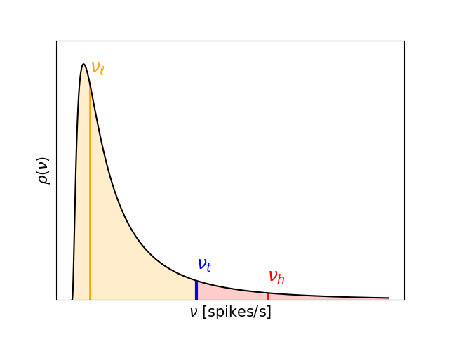
Figure 2: Log-normal distribution of firing rate. The black solid line indicated the probability distribution, which is divided into two sections by the rate threshold $\nu_{\text{t}}$ (blue, vertical line). The amber band represents the distribution of rate below the threshold, whose mean is $\nu_{\ell}$ (amber, vertical line). The red band represents the distribution of neurons whose rate is above threshold. Here the average of this section is $\nu_{\text{h}}$ (red, vertical line).

As in the discrete model, the test set consists of $V$ firing-rate patterns of the neurons of $\mathcal{P}_{1}$, randomly extracted from the $\mathcal{T}$ input patterns of the train set. Here we consider the case where the patterns are unchanged, thus each input patter of the test set is identical to an input pattern of the train set. In a later section we will discuss the effect of altering these patterns by adding noise. To estimate the values of $\langle\mathcal{S}_{\text{2}}\rangle$, $\langle\mathcal{S}_{\text{b}}\rangle$ and $\sigma^{2}_{\text{b}}$ we proceed in a similar way as for the discrete model. First of all we calculate the input signal to a generic non-coding neuron of $\mathcal{P}_{2}$. Let $\mathcal{C}$ be the number of incoming connections to this neuron, $P(k)$ the probability that $k$ of these connections are consolidated, $\nu_{1},\dotsi,\nu_{k}$ the firing rates of the presynaptic neurons of the consolidated connections and $\xi_{1},\dotsi,\xi_{\mathcal{C}-k}$ the firing rates of the presynaptic neurons of the unconsolidated connections. The probability of having $k$ consolidated connections and rates in the range $(\nu_{1},\nu_{1}+d\nu_{1}),\dotsi,(\nu_{k},\nu_{k}+d\nu_{k})$, $(\xi_{1},\xi_{1}+d\xi_{1}),\dotsi,(\xi_{\mathcal{C}-k},\xi_{\mathcal{C}-k}+d\xi_{\mathcal{C}-k})$ is $P(k)\rho(\nu_{1})\dotsi\rho(\nu_{k})\rho(\xi_{1})\dotsi\rho(\xi_{\mathcal{C}-k})d\nu_{1}\dotsi d\nu_{k}d\xi_{1}\dotsi d\xi_{\mathcal{C}-k}$. To calculate the average background signal we should average the expression of $\mathcal{S}_{\text{b}}$, given by equation 5, over all the possible values of $k$ and of the firing rates, thus

$$\begin{split}\langle\mathcal{S}_{\text{b}}\rangle&=\sum_{k}P(k)\int d\nu_{1}\dotsi\int d\nu_{k}\int d\xi_{1}\dotsi\int d\xi_{\mathcal{C}-k}\rho(\nu_{1})\dotsi\rho(\nu_{k})\rho(\xi_{1})\dotsi\rho(\xi_{\mathcal{C}-k})\cdot\\ &\cdot\Bigl{[}\mathcal{W}_{\text{c}}(\nu_{1}+\dotsi+\nu_{k})+\mathcal{W}_{\text{b}}(\xi_{1}+\dotsi+\xi_{\mathcal{C}-k})\Bigr{]}=\\ &=\sum_{k}P(k)\Bigl{[}\mathcal{W}_{\text{c}}k\langle\nu\rangle+\mathcal{W}_{\text{b}}(\mathcal{C}-k)\langle\nu\rangle\Bigr{]}=[\mathcal{W}_{\text{c}}\langle k\rangle+\mathcal{W}_{\text{b}}(\mathcal{C}-\langle k\rangle)]\langle\nu\rangle\end{split}$$ (24)

where we used the fact that $\int\nu\rho(\nu)d\nu=\int\xi\rho(\xi)d\xi=\langle\nu\rangle$. Note that the result obtained in Equation 24 is the same as the one obtained for the discrete model (see Equation 6).

The variance of the background signal can be similarly derived:

$$\begin{split}\sigma^{2}_{\text{b}}&=\langle(\mathcal{S}_{\text{b}}-\langle\mathcal{S}_{\text{b}}\rangle)^{2}\rangle=\sum_{k}P(k)\int d\nu_{1}\dotsi\int d\nu_{k}\int d\xi_{1}\dotsi\int d\xi_{\mathcal{C}-k}\rho(\nu_{1})\dotsi\rho(\xi_{\mathcal{C}-k})\cdot\\ &\cdot\Bigl{[}\mathcal{W}_{\text{c}}\sum_{i=1}^{k}\nu_{i}+\mathcal{W}_{\text{b}}\sum_{i=1}^{\mathcal{C}-k}\xi_{i}-[\mathcal{W}_{\text{c}}\langle k\rangle+\mathcal{W}_{\text{b}}(\mathcal{C}-\langle k\rangle)]\langle\nu\rangle\Bigr{]}^{2}=\\ &=\sum_{k}P(k)\int d\nu_{1}\dotsi\int d\xi_{\mathcal{C}-k}\rho(\nu_{1})\dotsi\rho(\xi_{\mathcal{C}-k})\Bigl{[}\mathcal{W}_{\text{c}}\sum_{i=1}^{k}(\nu_{i}-\langle\nu\rangle)+\mathcal{W}_{\text{b}}\sum_{i=1}^{\mathcal{C}-k}(\xi_{i}-\langle\nu\rangle)+\\ &+(k-\langle k\rangle)(\mathcal{W}_{\text{c}}-\mathcal{W}_{\text{b}})\langle\nu\rangle\Bigr{]}^{2}\end{split}$$ (25)

Where in the last line we used the substitution $\langle k\rangle=k+(\langle k\rangle-k)$ as done for Equation 10. The mixed terms of the equation above are null because $\int\rho(x)(x-\langle x\rangle)dx=0$, ergo we can write the variance of the background signal as follows:

$$\begin{split}\sigma^{2}_{\text{b}}&=\sum_{k}P(k)\int d\nu_{1}\dotsi\int d\xi_{\mathcal{C}-k}\rho(\nu_{1})\dotsi\rho(\xi_{\mathcal{C}-k})\Bigl{[}\mathcal{W}_{\text{c}}^{2}k\langle(\nu-\langle\nu\rangle)^{2}\rangle+\mathcal{W}_{\text{b}}^{2}(\mathcal{C}-k)\langle(\nu-\langle\nu\rangle)^{2}\rangle+\\ &+(\mathcal{W}_{\text{c}}-\mathcal{W}_{\text{b}})^{2}(k-\langle k\rangle)^{2}\langle\nu\rangle^{2}\Bigr{]}=\Bigl{[}\mathcal{W}_{\text{c}}^{2}\langle k\rangle+\mathcal{W}_{\text{b}}^{2}(\mathcal{C}-\langle k\rangle)\Bigr{]}\sigma_{\nu}^{2}+(\mathcal{W}_{\text{c}}-\mathcal{W}_{\text{b}})^{2}\sigma_{k}^{2}\langle\nu\rangle^{2}\end{split}$$ (26)

The variance of $k$ has the same expression as for the discrete case, and is derived in Appendix B. $\mathcal{S}_{\text{2}}$ can be derived similarly to the discrete case as well. We have a contribution from $p_{1}\mathcal{C}$ neurons of $\mathcal{P}_{1}$ at high rate connected by consolidated connections. The remaining $\mathcal{C}^{\prime}=\mathcal{C}-p_{1}\mathcal{C}$ neurons have a low rate and can be connected either by unconsolidated connections or by connections that have been consolidated in input patterns different from the current one. Calling $\langle k^{\prime}\rangle$ the average number of consolidated connections outgoing from the $\mathcal{C}^{\prime}$ low-rate neurons and using the definition of $\langle\nu_{\ell}\rangle$ and $\langle\nu_{\text{h}}\rangle$ given by Equation 22 we can write

$$\begin{split}\langle\mathcal{S}_{\text{2}}\rangle&=\mathcal{W}_{\text{c}}p_{1}\mathcal{C}\langle\nu_{\text{h}}\rangle+(\mathcal{W}_{\text{c}}-\mathcal{W}_{\text{b}})\langle k^{\prime}\rangle\langle\nu_{\ell}\rangle+\mathcal{W}_{\text{b}}\mathcal{C}(1-p_{1})\langle\nu_{\ell}\rangle=\\ &=\mathcal{W}_{\text{c}}p_{1}\mathcal{C}\langle\nu_{\text{h}}\rangle+\Bigl{[}(\mathcal{W}_{\text{c}}-\mathcal{W}_{\text{b}})\langle k\rangle+\mathcal{C}\mathcal{W}_{\text{b}}\Bigr{]}(1-p_{1})\langle\nu_{\ell}\rangle\end{split}$$ (27)

where we used the expression of $\langle k^{\prime}\rangle$ from Equation 12. As can be seen, Equation 27 differs from 13 only because the rates are not discrete but can assume continuous values, thus the discrete values $\nu_{\text{h}}$ and $\nu_{\ell}$ are replaced by the averages $\langle\nu_{\text{h}}\rangle$ and $\langle\nu_{\ell}\rangle$. The modified formula of $\mathcal{S}_{\text{2}}$ that takes into account connection rewiring will be derived in section II.1.4.

In this work we use a log-normal distribution of the firing rates for the continuous model. Indeed, it is known that rate distribution in the cortex are long-tailed and skewed with a log-normal shape [35]. The log-normal distribution is a continuous probability distribution of a random variable $\nu$ whose logarithm $\ln(\nu)$ is normally distributed. The probability density function of this distribution is

$$\rho_{\text{LN}}(\nu)=\frac{1}{\sqrt{2\pi}\sigma\nu}\cdot\exp\Bigl{(}-\frac{(\ln(\nu)-\mu)^{2}}{2\sigma^{2}}\Bigr{)}$$ (28)

where $\mu$ and $\sigma$ are the mean and standard deviation of $\ln(\nu)$. The expressions of the mean value and standard deviation of $\rho_{\text{LN}}(\nu)$ will be derived in Appendix A.

II.1.3 Poisson distribution of incoming connections per neuron

Hitherto we considered a model in which each neuron of $\mathcal{P}_{2}$ has a fixed number of incoming connections, i.e., a fixed in-degree, $\mathcal{C}$. However, a more general and more realistic approach would consider $\mathcal{C}$ as variable across the neurons of $\mathcal{P}_{2}$ according to an appropriate probability distribution $P(\mathcal{C})$. In this work we will focus on the case where the number of incoming connections follows a Poisson distribution (i.e. a Poisson-indegree connection rule), however the approach we will present can be easily extended to other distributions. The values of $\langle\mathcal{S}_{\text{2}}\rangle$ and $\langle\mathcal{S}_{\text{b}}\rangle$, previously averaged over the rate $\nu$ and the number of consolidated connections $k$, should be also averaged over the number of incoming connections, so that

$$\begin{split}\langle\langle\mathcal{S}_{\text{b}}\rangle_{\nu,k}\rangle_{\mathcal{C}}&=\sum_{c}P(\mathcal{C})\langle\mathcal{S}_{\text{b}}\rangle_{\nu,k}\\ \langle\langle\mathcal{S}_{\text{2}}\rangle_{\nu,k}\rangle_{\mathcal{C}}&=\sum_{\mathcal{C}}P(\mathcal{C})\langle\mathcal{S}_{\text{2}}\rangle_{\nu,k}\end{split}$$ (29)

where $\langle\mathcal{S}_{\text{2}}\rangle_{\nu,k}$ is given by Equation 27 and $\langle\mathcal{S}_{\text{b}}\rangle_{\nu,k}$ is given by Equation 24. Since these equations are linear in $\mathcal{C}$ and since $\sum_{\mathcal{C}}\mathcal{C}P(\mathcal{C})=\langle\mathcal{C}\rangle$, Equations 27 and 24 would show $\langle\mathcal{C}\rangle$ instead of $\mathcal{C}$ when averaged over the number of incoming connections per neuron.
The variance can be obtained from the equation:

$$\text{Var}(\langle\langle\mathcal{S}_{\text{b}}\rangle_{\nu,k}\rangle_{\mathcal{C}})=\sigma^{2}_{\nu,k,\mathcal{C}}=\langle\langle\mathcal{S}_{\text{b}}^{2}\rangle_{\nu,k}\rangle_{\mathcal{C}}-\langle\langle\mathcal{S}_{\text{b}}\rangle_{\nu,k}\rangle_{\mathcal{C}}^{2}$$ (30)

Knowing that $\langle\sigma^{2}_{\text{b}}\rangle_{\mathcal{C}}=\langle\langle\mathcal{S}_{\text{b}}^{2}\rangle_{\nu_{k}}-\langle\mathcal{S}_{\text{b}}\rangle_{\nu,k}^{2}\rangle_{\mathcal{C}}=\langle\langle\mathcal{S}_{\text{b}}^{2}\rangle_{\nu,k}\rangle_{\mathcal{C}}-\langle\langle\mathcal{S}_{\text{b}}\rangle_{\nu,k}^{2}\rangle_{\mathcal{C}}$ and that $\langle k\rangle=p\mathcal{C}$ we can write

$$\begin{split}\sigma^{2}_{\nu,k,\mathcal{C}}&=\langle\sigma^{2}_{\text{b}}\rangle_{\mathcal{C}}+\langle\langle\mathcal{S}_{\text{b}}\rangle_{\nu,k}^{2}\rangle_{\mathcal{C}}-\langle\langle\mathcal{S}_{\text{b}}\rangle_{\nu,k}\rangle_{\mathcal{C}}^{2}=\\ &=\langle\sigma^{2}_{\text{b}}\rangle_{\mathcal{C}}+\Bigl{\{}\langle\nu\rangle\Bigl{[}\mathcal{W}_{\text{b}}+p(\mathcal{W}_{\text{c}}-\mathcal{W}_{\text{b}})\Bigr{]}\Bigr{\}}^{2}\Bigl{[}\langle\mathcal{C}^{2}\rangle-\langle\mathcal{C}\rangle^{2}\Bigr{]}=\\ &=\langle\sigma^{2}_{\text{b}}\rangle_{\mathcal{C}}+\langle\nu\rangle^{2}\Bigl{[}\mathcal{W}_{\text{b}}+p(\mathcal{W}_{\text{c}}-\mathcal{W}_{\text{b}})\Bigr{]}^{2}\sigma_{\mathcal{C}}^{2}\end{split}$$ (31)

This equation is also valid for the discrete model.

II.1.4 Connection Rewiring

In the proposed approach, rewiring is implemented by periodically pruning unconsolidated connections and creating new ones. These procedures are performed with a fixed step on the number of training examples, which we will call rewiring step, denoted by the letter $s$. The creation of the new connections is made in such a way as to keep the distribution of the number of incoming connections per neuron unchanged. If $h$ is the number of consolidated incoming connections of a neuron of $\mathcal{P}_{2}$, after pruning all the unconsolidated connections, $\mathcal{C}-h$ new connections will be created. $\mathcal{C}$ is a fixed number if the fixed-indegree connection rule is used, while it is extracted from a Poisson distribution if the Poisson-indegree rule is selected; in both cases, the presynaptic neurons are randomly extracted from $\mathcal{P}_{1}$. For this reason, rewiring leaves the expressions of the background signal and of the variance on this signal unchanged, while, as we will see, it modifies the input signal to coding neurons. A diagram of the rewiring process is shown in Figure 3, which illustrates the activity of a high-rate neuron of $\mathcal{P}_{2}$ and of the presynaptic neurons of its incoming connections in a training example, and the effect of connection rewiring.

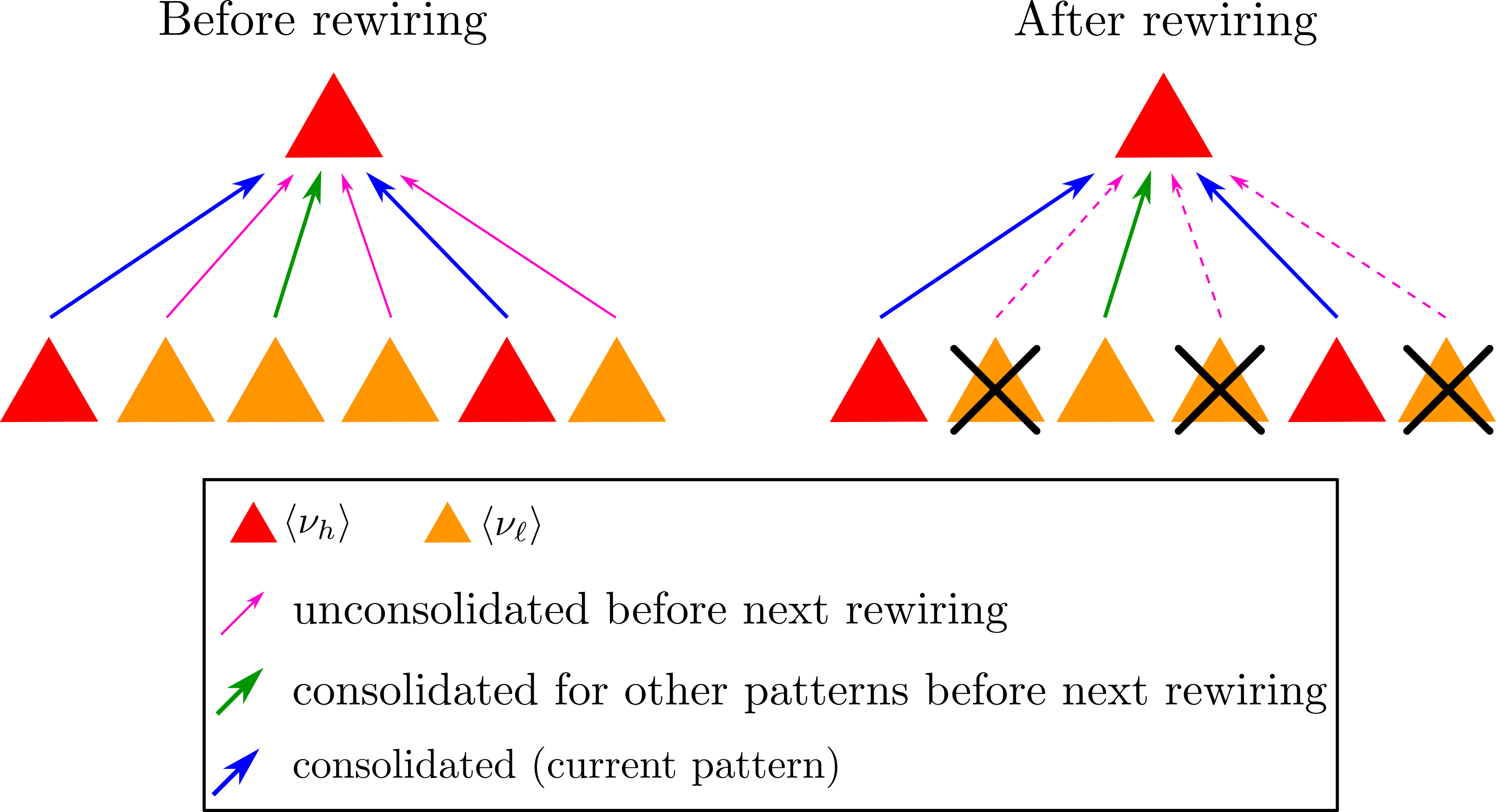
Figure 3: Schematization of the rewiring process and of its effect on the average signal in input to coding neurons of the population $\mathcal{P}_{2}$. Red and amber triangles represent high and low rate neurons respectively. Blue and green connections are consolidated for the current example and for a previous example, whereas pink connections are not consolidated. After rewiring these connections are pruned (here indicated with a dotted arrow), thus the relative presynaptic neurons do not project anymore to the postsynaptic neuron in exam.

The average number of incoming connections that are consolidated in the current example (blue lines) is equal to the average number of high-rate presynaptic neurons, $p_{1}\mathcal{C}$. The average number of incoming connections that are consolidated in other examples after the entire training, $\langle k^{\prime}\rangle$, is given by equation 12:

$$\langle k^{\prime}\rangle=p\mathcal{C}(1-p_{1})$$ (32)

Let $t$ be the next training index for which rewiring will be applied, and $k^{\prime}_{t}$ the number of connections from low-rate neurons that are consolidated before $t$ (green lines in the figure). These connections will not be affected by rewiring, so even in the test phase with the same input pattern they will have low-rate presynaptic neurons. The average value of $k^{\prime}_{t}$ is

$$\langle k^{\prime}_{t}\rangle=p_{t}\mathcal{C}(1-p_{1})$$ (33)

where $p_{t}$ is given by an expression analogous to the one obtained for $p$ (Equation 2)

$$p_{t}=1-(1-p_{1}p_{2})^{t}$$ (34)

On the other hand, there will be $k^{\prime}-k^{\prime}_{t}$ connections displaced by rewiring and consolidated in training examples of index greater than $t$. Putting all the contributions together, we obtain the following expression for $\mathcal{S}_{\text{2}}$:

$$\begin{split}\langle\mathcal{S}_{\text{2}}\rangle&=p_{1}\mathcal{C}\mathcal{W}_{\text{c}}\langle\nu_{\text{h}}\rangle+(\langle k^{\prime}\rangle-\langle k^{\prime}_{t}\rangle)\mathcal{W}_{\text{c}}\langle\nu\rangle+\langle k^{\prime}_{t}\rangle\mathcal{W}_{\text{c}}\langle\nu_{\ell}\rangle+\mathcal{W}_{\text{b}}(\mathcal{C}-p_{1}\mathcal{C}-\langle k^{\prime}\rangle)\langle\nu\rangle=\\ &=p_{1}\mathcal{C}\mathcal{W}_{\text{c}}\langle\nu_{\text{h}}\rangle+\langle k^{\prime}\rangle\mathcal{W}_{\text{c}}\langle\nu\rangle+\mathcal{W}_{\text{b}}[\mathcal{C}(1-p_{1})-\langle k^{\prime}\rangle]\langle\nu\rangle-\langle k^{\prime}_{t}\rangle\mathcal{W}_{\text{c}}(\langle\nu\rangle-\langle\nu_{\ell}\rangle)\end{split}$$ (35)

To obtain the average value of $\mathcal{S}_{\text{2}}$ over all examples, $\langle k^{\prime}_{t}\rangle$ must be averaged over all values of the index $t$ for which rewiring is done. This calculation is shown in Appendix D. Equation 35 is also valid in the case for which neurons can assume discrete values of firing rate. In that case, $\langle\nu_{\ell}\rangle$, $\langle\nu_{\text{h}}\rangle$ and $\langle\nu\rangle$ have to be replaced with the discrete values $\nu_{\ell}$, $\nu_{\text{h}}$ and the average rate $\langle\nu\rangle$ shown in Table 3.

II.1.5 Introduction of noise into input patterns

In a realistic learning model, the test patterns will never be exactly the same as the training ones. The ability of a learning model to generalize is linked to the ability to recognize which training pattern or patterns are most similar to a given test pattern, according to appropriate metrics. To study the generalization capacity of the model proposed in this work, the test input patterns were generated starting from the corresponding training input patterns by adding noise, which is represented by a deviation extracted from a given probability distribution with assigned standard deviation. In Appendix C we describe the effect that a noise with a truncated Gaussian distribution has on the firing rates and on the variables $\mathcal{S}_{\text{b}}$, $\mathcal{S}_{\text{2}}$, $\sigma^{2}_{\text{b}}$ and SDNR, and we derive the modified equations.

II.1.6 Summary of theoretical model equations

Table 4 summarizes the equations of the continuous rate model in case of fixed number of incoming connections per neuron. As mentioned before, when the value of $\mathcal{C}$ follows a Poisson distribution, $\langle\mathcal{S}_{\text{b}}\rangle$ and $\langle\mathcal{S}_{\text{2}}\rangle$ are given by the same expression obtained for the fixed in-degree connection rule with $\mathcal{C}$ replaced by $\langle\mathcal{C}\rangle$. The variance of the background signal has an additional term in that case and is given by Equation 31.

Continuous rate model
Name	Symbol	Equation
Rate distribution	$\rho(\nu)$	$\frac{1}{\sqrt{2\pi}\sigma\nu}\cdot\exp\Bigl{(}-\frac{(\ln(\nu)-\mu)^{2}}{2\sigma^{2}}\Bigr{)}$
Mean of the normal distribution of $\ln(\nu)$	$\mu$	$\ln(\langle\nu\rangle)-\frac{\sigma^{2}}{2}$
Standard deviation of the normal distribution of $\ln(\nu)$	$\sigma$	$\text{erf}^{-1}(q_{1})-\text{erf}^{-1}\Big{(}\frac{q_{1}\langle\nu_{\ell}\rangle}{\langle\nu\rangle}\Big{)}$
Rate threshold	$\nu_{\text{t}}$	$\exp\Big{(}\text{erf}^{-1}(q_{1})\sigma+\mu\Big{)}$
Average high rate	$\langle\nu_{\text{h}}\rangle$	$\frac{1}{p_{1}}\int_{\nu_{\text{t}}}^{\infty}\nu\rho(\nu)d\nu$
Average low rate	$\langle\nu_{\ell}\rangle$	$\frac{1}{q_{1}}\int_{0}^{\nu_{\text{t}}}\nu\rho(\nu)d\nu$
Average rate	$\langle\nu\rangle$	$q_{1}\langle\nu_{\ell}\rangle+p_{1}\langle\nu_{\text{h}}\rangle$
Rate standard deviation	$\sigma_{\nu}^{2}$	$\Big{(}e^{\sigma^{2}}-1\Big{)}e^{2\mu+\sigma^{2}}$
Average background signal	$\langle\mathcal{S}_{\text{b}}\rangle$	$(\mathcal{W}_{\text{c}}-\mathcal{W}_{\text{b}})\langle k\rangle\langle\nu\rangle+\mathcal{W}_{\text{b}}\mathcal{C}\langle\nu\rangle$
Variance of background signal	$\sigma^{2}_{\text{b}}$	$\Bigl{[}\mathcal{W}_{\text{c}}^{2}\langle k\rangle+\mathcal{W}_{\text{b}}^{2}(\mathcal{C}-\langle k\rangle)\Bigr{]}\sigma_{\nu}^{2}+(\mathcal{W}_{\text{c}}-\mathcal{W}_{\text{b}})^{2}\sigma_{k}^{2}\langle\nu\rangle^{2}$
Average coding-neuron signal (without rewiring)	$\langle\mathcal{S}_{\text{2}}\rangle$	$\mathcal{W}_{\text{c}}p_{1}\mathcal{C}\langle\nu_{\text{h}}\rangle+\Bigl{[}(\mathcal{W}_{\text{c}}-\mathcal{W}_{\text{b}})\langle k\rangle+\mathcal{C}\mathcal{W}_{\text{b}}\Bigr{]}(1-p_{1})\langle\nu_{\ell}\rangle$
Average coding-neuron signal (with rewiring)	$\langle\mathcal{S}_{\text{2}}\rangle$	$\mathcal{W}_{\text{c}}p_{1}\mathcal{C}\langle\nu_{\text{h}}\rangle+\Bigl{[}(\mathcal{W}_{\text{c}}-\mathcal{W}_{\text{b}})\langle k\rangle+\mathcal{C}\mathcal{W}_{\text{b}}\Bigr{]}(1-p_{1})\langle\nu\rangle-\langle k^{\prime}_{t}\rangle\mathcal{W}_{\text{c}}(\langle\nu\rangle-\langle\nu_{\ell}\rangle)$

Table 4: Summary of the equations for the continuous model. Equations shown here refers to the case in which the number of incoming connections per neuron $\mathcal{C}$ is constant.

II.2 Computational simulations of the model

The validation of the equations derived in the previous sections was done through simulations with firing-rate-based neuronal network models. The code of the simulator was written in the C++ programming language GCC (https://github.com/gcc-mirror/gcc) (version 10.2.0) and with the GSL (https://www.gnu.org/software/gsl/) (version 2.7) scientific libraries. The simulations have been performed using the supercomputers Galileo 100 and JUSUF [44]. The networks used for the simulations are generated according to the selected connection rule. In particular, in the case of the fixed-indegree rule, $\mathcal{C}$ incoming connections are created for each neuron of the $\mathcal{P}_{2}$ population, where $\mathcal{C}$ has a fixed value. In the case of the Poisson-indegree rule, for each neuron of the population $\mathcal{P}_{2}$ the number of incoming connections $C$ is extracted from a Poisson distribution with mean $\langle C\rangle$. In both cases, the indexes of the presynaptic neurons are randomly extracted on the $\mathcal{P}_{1}$ population. The connection weights are initially set to the baseline value, $\mathcal{W}_{\text{b}}$. Each training input patterns of the discrete model is generated by extracting, for each neuron of $\mathcal{P}_{1}$, a random number $r$ from a uniform distribution in the interval $[0,1]$; if $r<p_{1}$ the rate of the neuron is set to the high level, $\nu_{\text{h}}$, otherwise it is set to $\nu_{\ell}$. An analogous procedure is used to generate the corresponding contextual stimulus pattern on the neurons of the population $\mathcal{P}_{2}$. A connection is consolidated in a training example if both the presynaptic and the postsynaptic neuron are in the high-rate level, $\nu_{\text{h}}$. In the continuous case, the firing rates of the input pattern and those of the contextual pattern are extracted from a log-normal distribution. In this case, a connection is consolidated if the firing rates of both the presynaptic and postsynaptic neurons are above the thresholds $\nu_{t,1}$ and $\nu_{t,2}$, respectively. Connection rewiring is performed every $s$ training steps, as described in section II.1.4. The test set is generated by randomly extracting $V$ input patterns from the train set. In the discrete case, the patterns are not modified. In the continuous case, the patterns of the test set are altered by adding noise extracted from a truncated Gaussian distribution.

To estimate $\langle\mathcal{S}_{\text{b}}\rangle$ and $\langle\mathcal{S}_{\text{2}}\rangle$ we compute the input of each $\mathcal{P}_{2}$ neuron as the sum of the rate of the presynaptic neurons of its incoming connections multiplied by the synaptic weights (i.e., $\mathcal{W}_{\text{c}}$ or $\mathcal{W}_{\text{b}}$). The variance $\sigma^{2}_{\text{b}}$ is evaluated by the formula:

$$\sigma^{2}_{\text{b}}=\langle\mathcal{S}_{\text{b}}^{2}\rangle-\langle\mathcal{S}_{\text{b}}\rangle^{2}$$ (36)

where the mean values are calculated over the input signals to all non-coding neurons of $\mathcal{P}_{2}$.

III Results

This section compares the results of the simulations of the firing rate model with the theoretical predictions described in the previous section. Since we proposed several versions of the model, with different features implemented, the section is divided into different parts that sum up the main characteristics of the model. We present the results of the approaches employing discrete and continuous values for neuron firing rates, comparing the theoretical values of the average input signal to background neurons $\langle\mathcal{S}_{\text{b}}\rangle$, the average input signal to coding neurons $\langle\mathcal{S}_{\text{2}}\rangle$, the variance of the background input signal $\sigma^{2}_{\text{b}}$ and the signal-difference-to-noise ratio with the values obtained from the simulations. This way, we are able to assess the capacity of the population $\mathcal{P}_{2}$, and thus of the network, to recognize a pattern memorized in the training phase. Here, we present simulation results with a Poisson-driven number of incoming connections, with $\langle\mathcal{C}\rangle=5000$. We opted for such an approach since it is more realistic for biological neural circuits with respect to a fixed amount of connections per neuron. Each simulation is repeated $10$ times using a different seed for random number generation to ensure the robustness of the simulation results. The values shown in the plots are a result of averaging over the different seeds.

III.1 Comparison between continuous and discrete firing rate

As previously mentioned, the main difference in calculating $\langle\mathcal{S}_{\text{b}}\rangle$ and $\langle\mathcal{S}_{\text{2}}\rangle$ with the continuous rate model versus the discrete model is that the discrete values of $\nu_{l}$ and $\nu_{h}$ are replaced, respectively, by the average values of the rate below and above threshold, calculated on the continuous probability distribution. On the other hand, the variance of the background signal differs in the two models, because it depends on the variance of the rate, $\sigma^{2}_{\nu}$, which is different in the two cases.
The first study we present is oriented towards the estimation of these parameters as a function of the number of training patterns $\mathcal{T}$. As the number of training patterns increases, so does the number of patterns encoded by each individual neuron. Since $p_{2}$ is the probability that a neuron of $\mathcal{P}_{2}$ is in a high-rate level for a single training pattern, on average such neuron will encode $p_{2}\mathcal{T}$ patterns of the entire training set. This multiple selectivity of individual neurons is also present in biological neural networks, in which the same neuron can be selective for several stimuli [34].
The test set consists of $V=1000$ input patterns, generated as described in the Materials and Methods section. Thus, the simulation outcome used for our analysis is an average over the entire test set of the $\mathcal{S}_{\text{b}}$, $\mathcal{S}_{\text{2}}$, $\sigma^{2}_{\text{b}}$ and SDNR values obtained for each test pattern. Figure 4 shows the comparison of the simulation outcomes using discrete and continuous rate values.

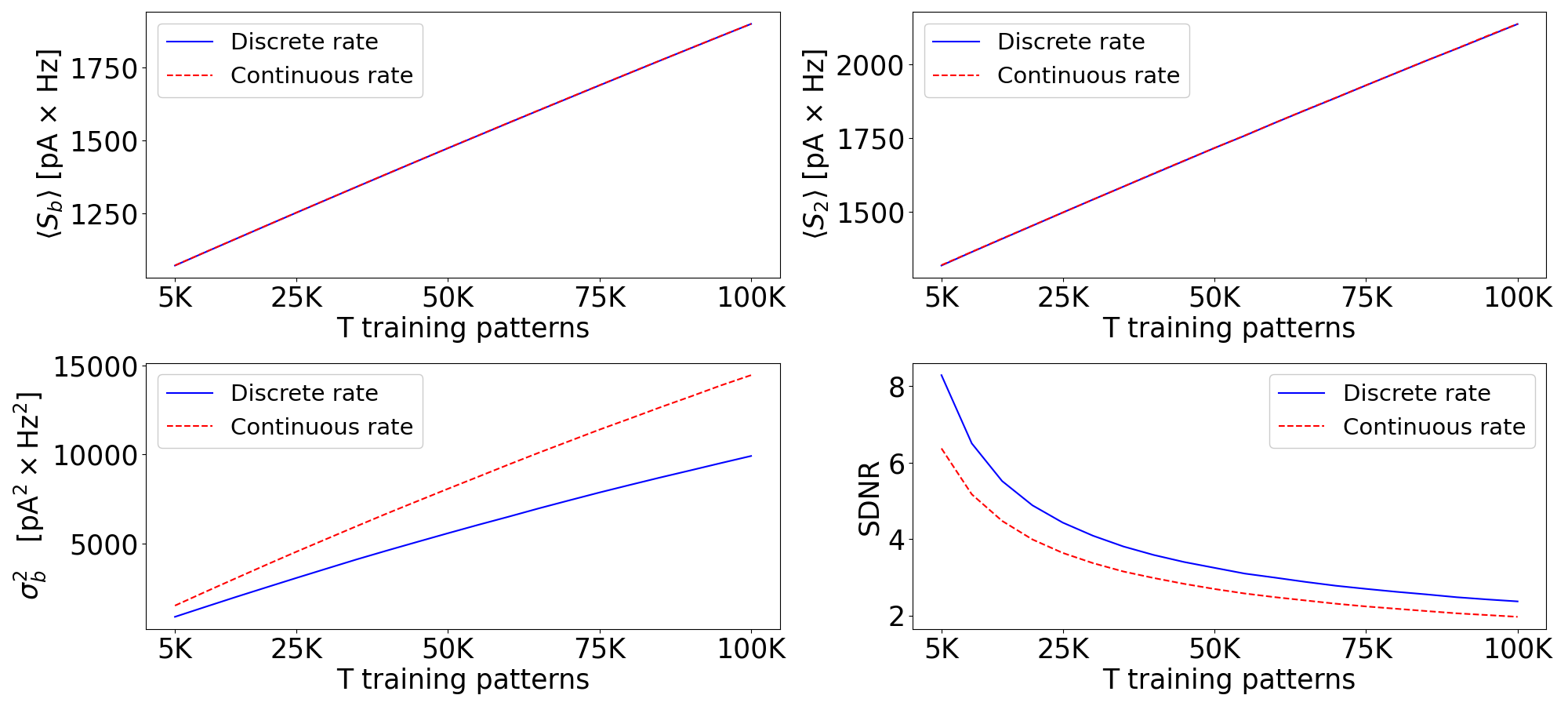
Figure 4: Comparison between $\langle\mathcal{S}_{\text{b}}\rangle$, $\langle\mathcal{S}_{\text{2}}\rangle$, $\sigma^{2}_{\text{b}}$ and SDNR obtained from simulations using discrete (blue line) or continuous (red dotted line) firing rate distribution. The values are given as a function of the number of training patterns $\mathcal{T}$.

We can see that the curves of $\langle\mathcal{S}_{\text{b}}\rangle$ and $\langle\mathcal{S}_{\text{2}}\rangle$ obtained from the simulations using the continuous firing rate distribution are superimposed on those obtained using the discrete model; this is due to the fact that the the choice of the threshold on the log-normal distribution is done so that the average values for low and high rate, $\langle\nu_{l}\rangle$ and $\langle\nu_{h}\rangle$, correspond to the values adopted in the discrete rate model. On the other hand, the variance of the background signal $\sigma^{2}_{\text{b}}$ differs in the two models, because it depends on the variance of the firing rate, $\sigma_{\nu}$, which is different in the two cases. This leads also to the different behavior of the SDNR.

III.2 Comparison between theoretical predictions and simulation results

The results shown in the previous section are obtained from simulations. This section presents a comparison between simulation results and theoretical expectations. To provide a quantitative estimation of the discrepancy between the theoretical predictions and the simulations, we evaluate their relative error, using the theoretical values as a reference.
As described previously, the test input patterns used in the continuous rate model are altered from the corresponding training input patterns by adding noise extracted from a truncated Gaussian distribution, with assigned standard deviation. In this section, we present simulation results and comparisons with theoretical predictions for standard deviation values ranging from $1$ Hz to $5$ Hz. These values are relatively high in relation to the average firing rate of $\mathcal{P}_{1}$, which is slightly higher than $2$ Hz.
Figure 5 shows the curves obtained for the continuous rate model using different values for the standard deviation of the noise, together with the relative error with respect to theoretical predictions. It can be observed that the curves obtained from the simulations are compatible with the theoretical ones for all the noise levels.

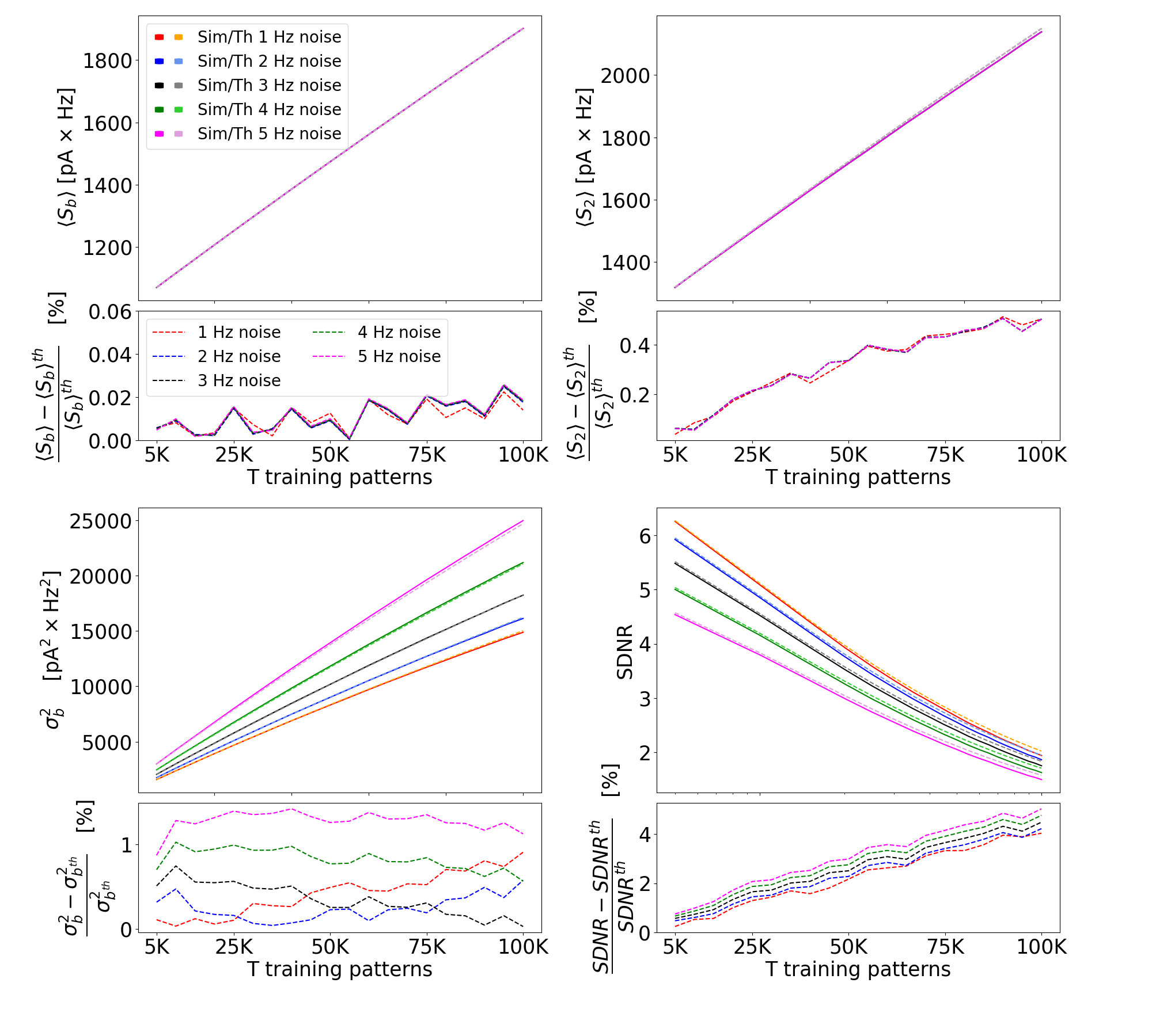
Figure 5: Values of $\langle\mathcal{S}_{\text{b}}\rangle$, $\langle\mathcal{S}_{\text{2}}\rangle$, $\sigma^{2}_{\text{b}}$ and the SDNR and percent error with respect to the theoretical prediction, as a function of the number of training patterns $\mathcal{T}$. Bigger subplots represent the values of the quantities considered as a function of $\mathcal{T}$ for different noise levels, whereas each smaller subplot represent the percentage error of the values shown in the upper subplot. The different color families identify the simulation and theory results when having a noise standard deviation of $1$ Hz (red-orange), $2$ Hz (blue-light blue), $3$ Hz (black-grey), $4$ Hz (green-light green) and $5$ Hz (magenta-pink).

Regarding $\langle\mathcal{S}_{\text{b}}\rangle$ and $\langle\mathcal{S}_{\text{2}}\rangle$, the curves corresponding to different noise levels appear perfectly superimposed. This is due to the fact that the noise is driven by a distribution with zero mean, and thus the addition of noise to the quantities represented in the curves does not alter their average (see Appendix C for the details). Regarding $\sigma^{2}_{\text{b}}$, the values corresponding to different noise levels differ from each other and increase with the standard deviation of the noise, in agreement with the theoretical model.
The relative error between simulation results and theoretical prediction is quite small: for $\langle\mathcal{S}_{\text{b}}\rangle$ and $\langle\mathcal{S}_{\text{2}}\rangle$ the errors span between $0.01$% and $0.4$%, whereas $\sigma^{2}_{\text{b}}$ shows a relative error of around $1$% for all the simulations performed with different number of training patterns.

The addition of noise with fluctuations greater than or comparable to the average firing rate can produce negative rate values for a fraction of the neurons. Considering that negative rate values are not physically possible, this behavior can be corrected in the simulations by simply replacing negative values of the firing rates with zero, i.e. saturating negative rates to zero. This correction is equivalent to having a different noise distribution, with an average value greater than zero. However, the current theoretical model is not able to take this effect into account. Since negative values are replaced by zeros, we would expect the average values of $\mathcal{S}_{\text{b}}$ and $\mathcal{S}_{\text{2}}$ evaluated by the simulations that exploit saturation to be greater than the values predicted by the theoretical model. Figure 6 shows the behavior of the model with this correction on the neurons firing rate.

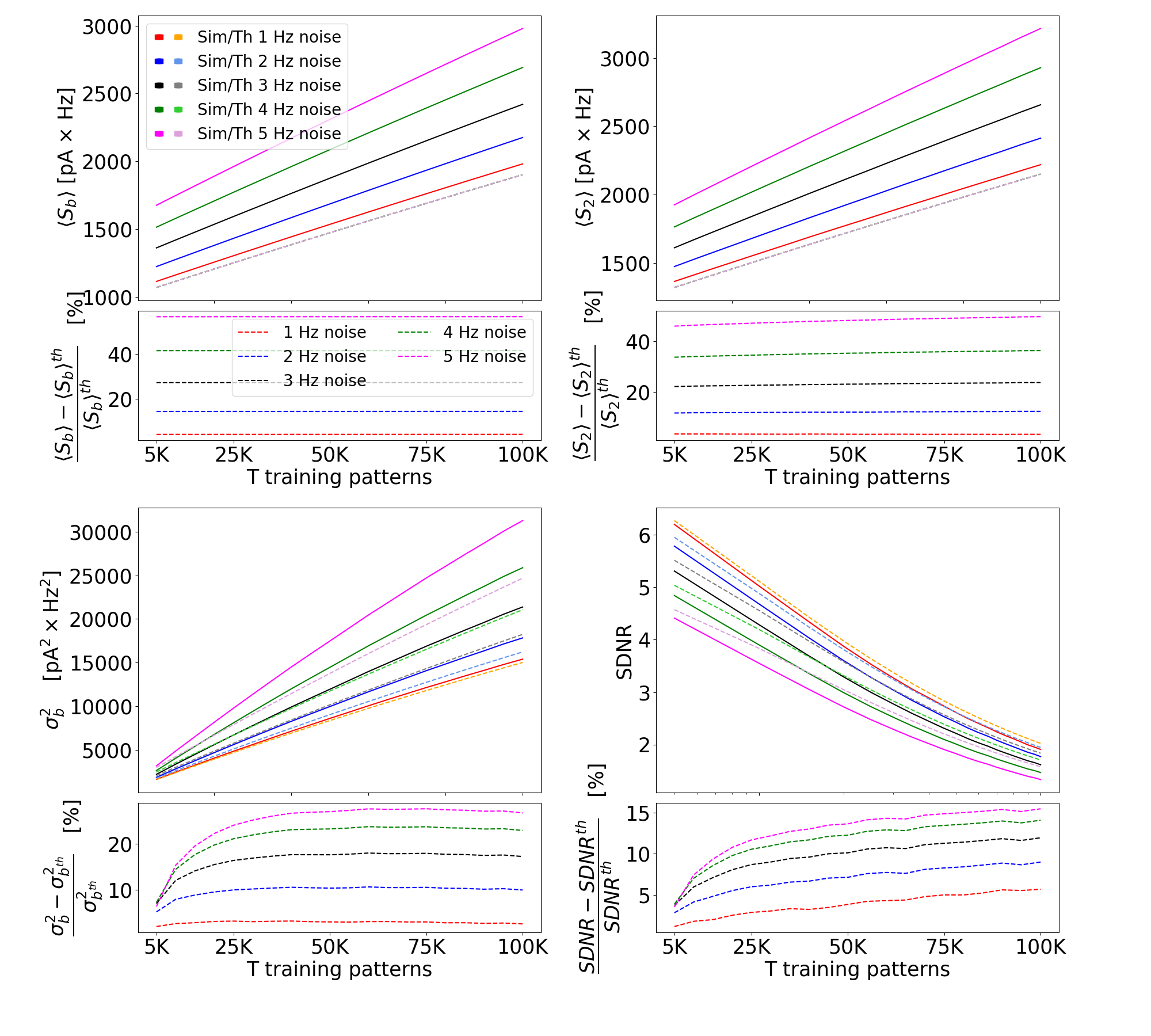
Figure 6: Values of $\langle\mathcal{S}_{\text{b}}\rangle$, $\langle\mathcal{S}_{\text{2}}\rangle$, $\sigma^{2}_{\text{b}}$ and SDNR, and percent error with respect to the theoretical predictions, as a function of the number of training patterns $\mathcal{T}$ when negative rates due to noise addition are saturated to zero. The different color families identify the simulation and theory results when having a noise standard deviation of $1$ Hz (red-orange), $2$ Hz (blue-light blue), $3$ Hz (black-grey), $4$ Hz (green-light green) and $5$ Hz (magenta-pink).

As can be seen from the figure, the discrepancies between simulations and theoretical predictions are much higher and can arrive to $40$%. This is due to the fact that the current theoretical framework is not able to take this correction into account. However it should be considered, as discussed above, that the considered noise levels are relatively high when compared with the average rate used in these simulations. Indeed, a different choice for the values of $\langle\nu_{\ell}\rangle$ and $\langle\nu_{\text{h}}\rangle$ (and thus a different average rate of the whole distribution) would have an impact on the discrepancies shown here. In particular, a higher average rate would strongly diminish the amount of neurons having negative firing rate as a result of the noise addition.

The relative error of $\sigma^{2}_{\text{b}}$ is greater than that shown for $\langle\mathcal{S}_{\text{b}}\rangle$ and $\langle\mathcal{S}_{\text{2}}\rangle$ in Figure 5; this is due to a simplification used in the theoretical model to derive the expression of the variance. The values of $\mathcal{S}_{\text{b}}$ from which we compute the variance are obtained by incoming connections from neurons of $\mathcal{P}_{1}$, but since connections are created randomly, different neurons of the $\mathcal{P}_{2}$ population may have presynaptic neurons in common, and therefore their input signals are correlated. The theoretical model does not take this correlation into account. The average number of presynaptic neurons in common to two arbitrary neurons of $\mathcal{P}_{2}$ depends on the total number of neurons of $\mathcal{P}_{1}$ and on the number of incoming connections per neuron of $\mathcal{P}_{2}$. Calling $\mathcal{N}_{1}=\mathcal{N}$, we can state that the bias due to this simplification becomes more and more relevant when the ratio $\mathcal{C}/\mathcal{N}$ increases. In order to estimate this bias as a function of the $\mathcal{C}/\mathcal{N}$ ratio, we performed a series of simulations with a fixed number of training patterns, $\mathcal{T}=5000$, changing the $\mathcal{C}/\mathcal{N}$ ratio. Figure 7 shows the results of this analysis.

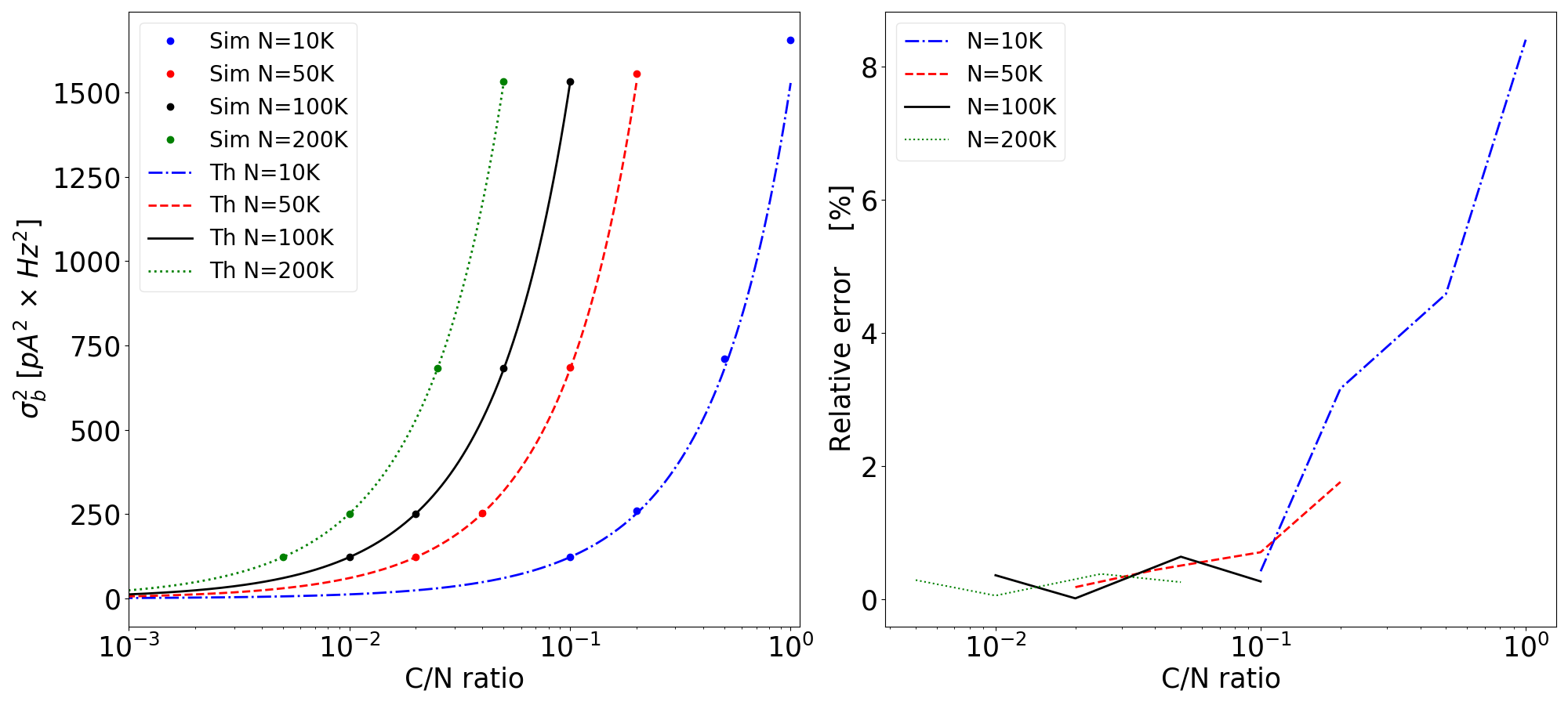
Figure 7: Values of $\sigma^{2}_{\text{b}}$ as a function of the $\mathcal{C}/\mathcal{N}$ ratio for different values of $\mathcal{N}$. On left panel, lines represent the theoretical prediction (Th), whereas dots represent the values obtained from the simulation (Sim). On the right panel, dotted lines represent the relative error between simulation results and theoretical prediction.

As can be seen in the right panel of Figure 7, a greater value of $\mathcal{C}/\mathcal{N}$ leads to a higher discrepancy between theoretical prediction and simulation. However, such a ratio, for natural density circuits in the brain, is very far from values of $\mathcal{C}/\mathcal{N}$ near unity. Indeed, a plausible value of the ratio would be less than $0.1$, resulting in negligible relative errors.

III.3 Impact of synaptic rewiring

In the simulations discussed so far, the rewiring mechanism was always performed with a rewiring step $s=100$. This means that every $100$ training patterns, all the unconsolidated connections are removed, and new connections are created. This operation represents the effect of homeostatic structural plasticity, that aims at keeping the network balanced by reorganizing connections, while activity-dependent structural plasticity focuses on the consolidation of connections.
To motivate the choice of this step for connection rewiring, we show here the results for networks trained for $\mathcal{T}=5000$ patterns with a different rewiring step $s$. We also show the results of a simulation that does not perform rewiring, in order to highlight the different behavior of a network that combines connection consolidation with periodic rewiring and that of a network that exploits only connection consolidation. Figure 8 shows the results obtained by these simulations using different rewiring intervals.

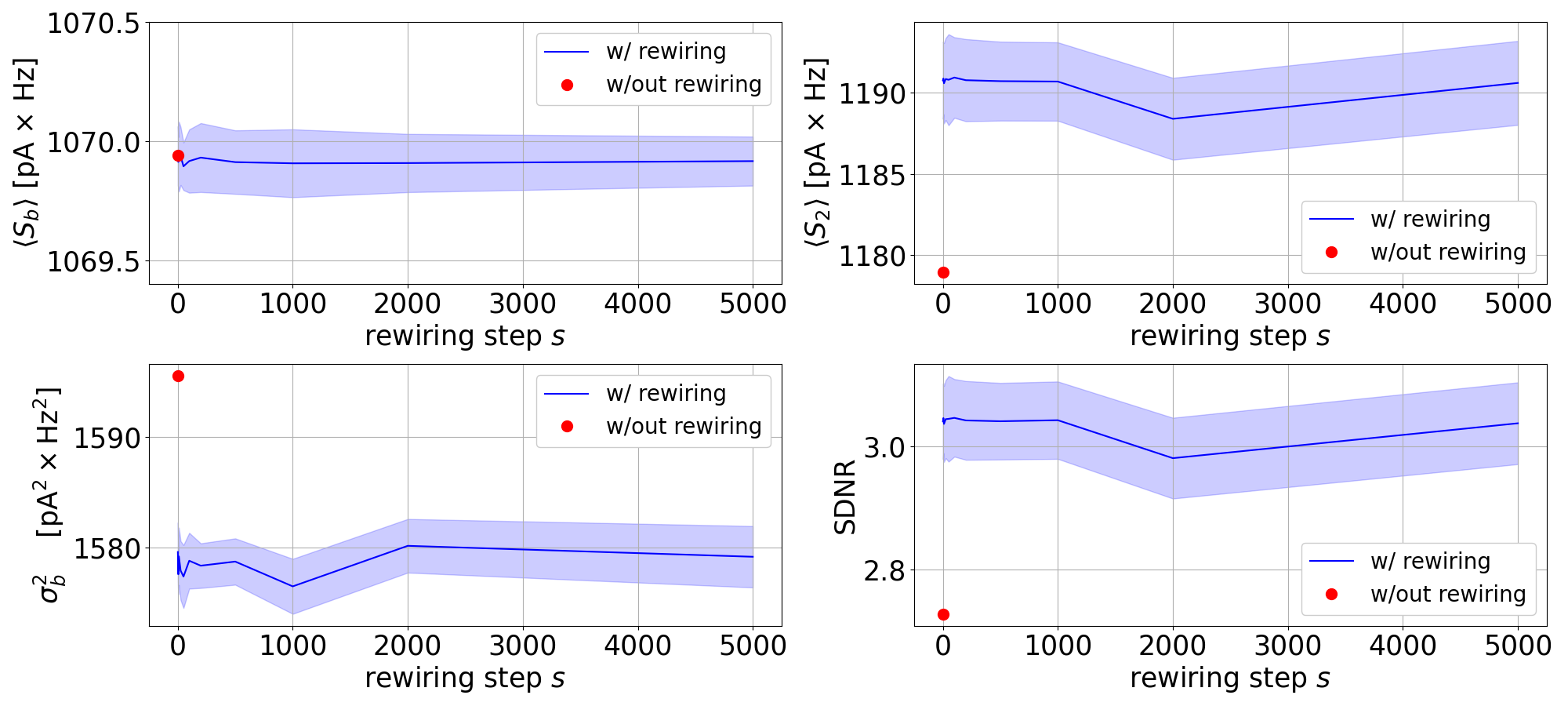
Figure 8: Values of $\langle\mathcal{S}_{\text{b}}\rangle$, $\langle\mathcal{S}_{\text{2}}\rangle$, $\sigma^{2}_{\text{b}}$ and SDNR for a network trained with $5000$ patterns as a function of the rewiring step $s$. The simulations used a continuous rate distribution and a noisy input driven by truncated Gaussian distribution with standard deviation of $1$ Hz. The red dot indicates the simulation outcome when connection rewiring is disabled, whereas the blue line shows the simulation results with connection rewiring, using different values of $s$. Blue shading represents the standard deviation of the mean obtained from $10$ simulations using different seeds for random number generation.

As can be noticed, the values of $\mathcal{S}_{\text{b}}$, $\mathcal{S}_{\text{2}}$, $\sigma^{2}_{\text{b}}$ and SDNR do not change significantly as the rewiring step varies. This means that the value of the step $s$ chosen for the connection rewiring has no impact in the results of the simulations. On the other hand, significant differences emerge when comparing the results of simulations with or without connection rewiring; it can be observed that the signal-difference-to-noise ratio has a lower value when the rewiring is disabled. This confirms that connection rewiring grants a higher capability of recognising an input pattern among the several patterns for which the network was trained.
We also applied a similar protocol for simulations enabling or disabling connection rewiring as a function of the number of training patterns $\mathcal{T}$. The results are shown in Figure 9.
We can say that the performance of the model are improved when connection rewiring is enabled, and the relative difference between a rewired or just consolidated connectivity increases when increasing the number of training patterns.
The effect of rewiring can become more relevant when a greater number of connections is consolidated at every step (i.e., with greater values of $p_{1}$ and $p_{2}$). Furthermore, the importance of the rewiring mechanisms can significantly change when the average number of connections is not constant, but increases or decreases as a result of rewiring itself. This aspect will be explored in a future work.

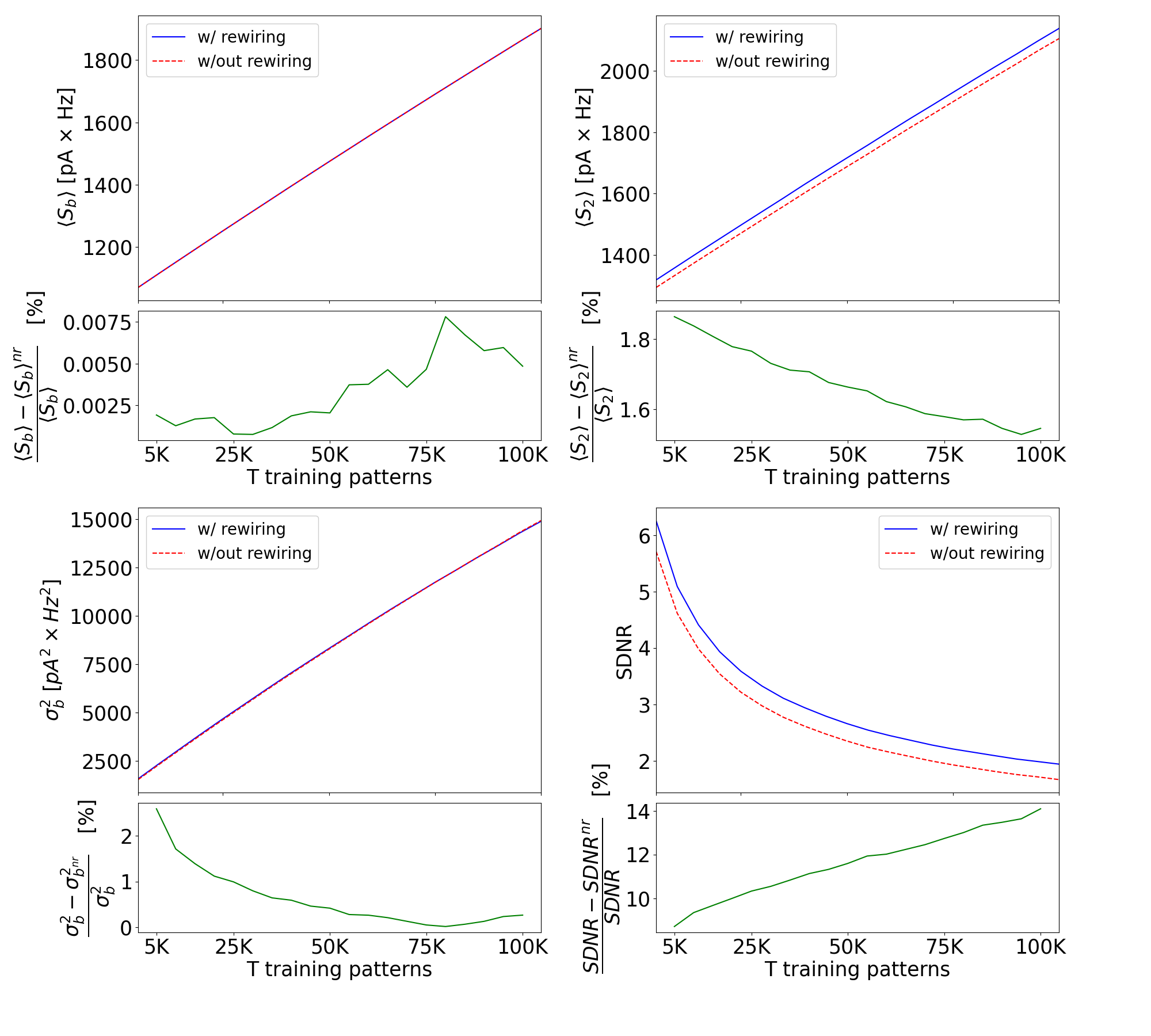
Figure 9: Comparison between simulations exploiting the connection rewiring mechanism performed every $100$ training patterns (blue lines) and simulations without rewiring (red lines) for a network trained with a variable number of training patterns $\mathcal{T}$. Green lines in the sub-panels show the difference between the values obtained with connections rewired or not rewired (indicated with $nr$) as percentage error.

IV Discussion

In the previous section the predictions of the theoretical framework, based on a mean-field approach, have been compared with the results of simulations performed using firing-rate-based neuronal networks. This comparison shows that the proposed framework is able to accurately predict the values of various quantities relevant for assessing learning and memory capacity in the presence of structural plasticity mechanisms, taking into account numerous characteristics of biological neuronal networks. The rates of neurons in the training and test patterns can be distributed according to an arbitrary probability distribution. In this work two cases have been considered, a simplified one in which the rates can assume only two values, high rate and low rate, and a more realistic one in which the rates follow a log-normal distribution in agreement with [35]. Connectivity between regions can be achieved through different connection rules, with fixed number of connections per target neuron or, more realistically, with a random connectivity in which the number of incoming connections of each target neuron follows a Poisson distribution.
Since the biochemical and biophysical mechanisms underlying structural plasticity are multiple and extremely complex, we opted for a phenomenological approach to capture their main aspects: a simple model of structural plasticity has been exploited, able to to represent plasticity processes driven by neuronal activity as well as mechanisms which leads to homeostasis, in agreement with the work of [11] which divides structural plasticity mechanisms in these two categories. Structural plasticity driven by neuronal activity is achieved through the consolidation of synapses connecting neurons that are concurrently in a high-rate level. This process can be triggered by other forms of plasticity that modify synaptic efficacy, such as STDP, followed by mechanisms involving citoarchitectural changes, such as the creation of novel connections next to the already existing ones.
The homeostatic form of structural plasticity involves a balance between pruning connections that are not utilized over time and creation of novel connections. This is achieved in the simulations through a periodic connection rewiring, which consists of a removal of unconsolidated connections followed by creation of new connections. The results show that connection rewiring leads to an increase in SDNR, conducting to an higher capability of recognizing the input patterns when this mechanism is enabled.
In order to evaluate the generalization capability of the framework with the continuous firing-rate distribution model, the test patterns were generated by altering the training input patterns through the addition of noise from a given probability distribution and assigned standard deviation. In particular, in this work a truncated Gaussian distribution has been used for the noise. The results of the simulations are compatible with the theoretical predictions, with differences in the order of $1-2$%, which is a remarkable result for our purpose.
Such an approach can lead to a fraction of the neurons with a negative firing rate as a result of noise addition. Since negative firing rates are not physically possible, a more realistic model would apply a saturation to zero for these rates. Saturation can be activated in the neuronal network simulations, however the current version of the theoretical framework is unable to account for it. This leads to a discrepancy between the simulations with saturation turned on and the theoretical predictions, which grows as the noise increases and becomes relevant when the noise gets significantly greater than the average firing rate. Future work should be devoted to the development of a theoretical model capable of taking into account the saturation of negative firing rates.
Another limitation of the framework comes from a simplification in the calculation of the background signal variance, which does not take into account the correlations between the contributions of presynaptic neurons to the input signals to distinct neurons of the target population. However, the results show that the impact of this simplifications is very small, at most in the order of a few percent.
The theoretical model can be surely extended. It can potentially provide a powerful tool to describe the impact of structural plasticity in cognitive processes such as learning in a large-scale model of the cortex with natural density and plausible characteristics. For instance, the consolidation mechanism can be probability-driven, with a probability depending on the rate of pre- and postsynaptic neurons. This would replace the current deterministic mechanism that requires a firing rate threshold to be exceeded from both the neurons to have synaptic consolidation. Moreover, the probability could depend on other variables not necessarily related to the firing rate. In particular, it has been hypothesized that plasticity mechanisms may also depend on the bursting activity of neurons [4, 31]. The consolidation probability of a connection could therefore depend, in addition to the firing rate of the presynaptic and postsynaptic neurons, also to their bursting activity.
In this work we have considered the connections between two distinct populations $\mathcal{P}_{1}$ and $\mathcal{P}_{2}$. However, the proposed framework also lends itself to the study of structural plasticity in the self-connections of a neuron population. An extension of the model could include recurrent connections in $\mathcal{P}_{2}$, together with an inhibitory population in order to have a more realistic architecture of excitatory and inhibitory neurons. Indeed, it is known that the mechanisms of competition through lateral inhibition play a key role in biological learning [10]. In this extended model, the theoretical framework can allow to obtain the differential equations governing the dynamics of the activity of the population $\mathcal{P}_{2}$ and the dependence of the coefficients of these equations on the number of training patterns and on the other model parameters [38]. Such an extension is currently under development and it will be subject of a future work.
Another extension of the model could describe more in detail the mechanisms of synaptic pruning and rewiring. Indeed, connection rewiring as intended in the current model preserves the total number of connections over time, which is a typical behavior of a healthy adult brain [20]. However, to shed light of the importance of these mechanism in neurological disorders, or to perform studies focused on this mechanism in different life stages, this mechanism should be extended to enable different ”speed” for the processes embedded in structural plasticity.
Moreover, it would be interesting to expand this work through simulations of spiking neural networks, to study learning through structural plasticity in more detail. Indeed, simulators such as NEST [13] and its GPU implementation [41] can lead to fast and efficient simulations of large-scale models on supercomputer clusters.
In conclusion, this work intend to provide a sufficiently general theoretical framework for learning through structural plasticity. This framework is able to describe synaptic consolidation, pruning and rewiring, and includes several features that can be added with a modular fashion. The validation has been performed through simulations with firing-rate-based neuronal network models, showing a remarkable compatibility between the results of the simulations and theoretical predictions.

Author contributions

Conceptualization: Bruno Golosio, Gianmarco Tiddia and Luca Sergi

Data curation: Bruno Golosio, Gianmarco Tiddia and Luca Sergi

Formal analysis: Bruno Golosio, Gianmarco Tiddia and Luca Sergi

Funding acquisition: Bruno Golosio

Investigation: Bruno Golosio, Gianmarco Tiddia and Luca Sergi

Methodology: Bruno Golosio, Gianmarco Tiddia and Luca Sergi

Project administration: Bruno Golosio

Resources: Bruno Golosio and Gianmarco Tiddia

Software: Bruno Golosio, Gianmarco Tiddia and Luca Sergi

Supervision: Bruno Golosio

Validation: Bruno Golosio, Gianmarco Tiddia and Luca Sergi

Visualization: Bruno Golosio, Gianmarco Tiddia and Luca Sergi

Writing - original draft: Bruno Golosio, Gianmarco Tiddia and Luca Sergi

Writing - review and editing: Bruno Golosio, Gianmarco Tiddia and Luca Sergi

Funding

This study was supported by the European Union’s Horizon 2020 Framework Programme for Research and Innovation under Specific Grant Agreements No. 945539 (Human Brain Project SGA3), No. 785907 (Human Brain Project SGA2), and by the Italian Ministry of University and Research (MUR) Piano Nazionale di Ripresa e Resilienza (PNRR), project e.INS Ecosystem of Innovation for Next Generation Sardinia – spoke 10 - CUP F53C22000430001 – MUR code: ECS00000038. We acknowledge the use of Fenix Infrastructure resources, which are partially funded from the European Union’s Horizon 2020 research and innovation programme through the ICEI project under the grant agreement No. 800858.

Data availability statement

All the simulation code needed to reproduce the results reported in this work, together with the related documentation, are freely available in the GitHub repository https://github.com/gmtiddia/structural_plasticity.

V Bibliography

Appendix A Log-normal distribution of the firing rate

The theoretical treatment of the continuous model proposed in this work is valid for a generic firing rate probability distribution. However, the model validation presented in the result section is focused on a log-normal distribution, which is a continuous probability distribution of a random variable $\nu$ whose logarithm $\ln(\nu)$ is normally distributed. The probability density function of this distribution is

$$\rho_{\text{LN}}(\nu)=\frac{1}{\sqrt{2\pi}\sigma\nu}\cdot\exp\Bigl{(}-\frac{(\ln(\nu)-\mu)^{2}}{2\sigma^{2}}\Bigr{)}$$ (37)

where $\mu$ and $\sigma$ are the mean and standard deviation of $\ln(\nu)$. Expanding Equation 22 using Equation 37 we have

$$\begin{split}\langle\nu_{\ell}\rangle&=\frac{1}{q_{1}}\int_{-\infty}^{y_{t}}\nu(y)G_{\sigma,\mu}(y)dy=\frac{1}{q_{1}}\int_{-\infty}^{y_{t}}e^{y}\frac{1}{\sqrt{2\pi\sigma^{2}}}e^{\frac{-(y-\mu)^{2}}{2\sigma^{2}}}dy\\ \langle\nu_{\text{h}}\rangle&=\frac{1}{p_{1}}\int_{y_{t}}^{\infty}\nu(y)G_{\sigma,\mu}(y)dy=\frac{1}{p_{1}}\int_{y_{t}}^{\infty}e^{y}\frac{1}{\sqrt{2\pi\sigma^{2}}}e^{\frac{-(y-\mu)^{2}}{2\sigma^{2}}}dy\end{split}$$ (38)

where $y$ is a variable representing the logarithm of the firing rate, $y=\ln(\nu)$, and follows a normal distribution $G_{\sigma,\mu}(y)$, while $y_{t}$ represents the value linked to the threshold value on the rate $\nu_{t}$ ($y_{t}=\ln(\nu_{t})$).

In the logarithmic representation the area of the portion of the Gaussian $G_{\sigma,\mu}(y)$ having $y<y_{t}$ corresponds to the probability that a neuron has a low rate, $q_{1}$. Therefore we can write:

$$q_{1}=\int_{-\infty}^{y_{t}}G_{\sigma,\mu}(y)dy=\frac{1}{2}+\int_{\mu}^{y_{t}}\frac{1}{\sqrt{2\pi\sigma^{2}}}e^{-\frac{(y-\mu)^{2}}{2\sigma^{2}}}dy$$ (39)

Substituting $x=\frac{y-\mu}{\sqrt{2}\sigma}$ we obtain:

$$q_{1}=\frac{1}{2}+\int_{0}^{\frac{y_{t}-\mu}{\sqrt{2}\sigma}}\frac{1}{\sqrt{\pi}}e^{-x^{2}}dx=\frac{1}{2}+\frac{1}{2}\text{erf}(\frac{y_{t}-\mu}{\sqrt{2}\sigma})$$ (40)

where with $\text{erf}(x)$ we indicate the error function, defined as:

$$\text{erf}(x)=\frac{2}{\sqrt{\pi}}\int_{0}^{x}e^{-t^{2}}dt$$ (41)

and then:

$$y_{t}=\mu+\sqrt{2}\sigma\text{erf}^{-1}(2q_{1}-1)$$ (42)

where $\text{erf}^{-1}$ is the inverse of the erf function. By substituting $z=y-\mu$ we can rewrite $\nu_{h}$ from Equation 38 as:

$$\begin{split}\langle\nu_{h}\rangle=&\frac{1}{p_{1}}\int_{y_{t}-\mu}^{\infty}\frac{1}{\sqrt{2\pi\sigma^{2}}}e^{z+\mu-\frac{z^{2}}{2\sigma^{2}}}dz=\frac{1}{p_{1}}\frac{e^{\mu}}{\sqrt{2\pi\sigma^{2}}}\int_{y_{t}-\mu}^{\infty}e^{-\frac{z^{2}-2\sigma^{2}z}{2\sigma^{2}}}dz=\\ =&\frac{1}{p_{1}}\frac{e^{\mu}}{\sqrt{2\pi\sigma^{2}}}\int_{y_{t}-\mu}^{\infty}e^{-\frac{(z-\sigma^{2})^{2}-\sigma^{4}}{2\sigma^{2}}}dz=\frac{1}{\sqrt{2\pi}}\frac{e^{\mu+\frac{\sigma^{2}}{2}}}{\sigma p_{1}}\int_{y_{t}-\mu}^{\infty}e^{\frac{-(z-\sigma^{2})^{2}}{2\sigma^{2}}}dz\end{split}$$ (43)

Making a further substitution $\xi=\frac{z-\sigma^{2}}{\sqrt{2}\sigma}$ finally we find:

$$\begin{split}\langle\nu_{h}\rangle&=\frac{1}{\sqrt{\pi}}\frac{e^{\mu+\frac{1}{2}\sigma^{2}}}{p_{1}}\int_{\frac{y_{t}-\mu-\sigma^{2}}{\sqrt{2}\sigma}}^{\infty}e^{-\xi^{2}}d\xi=\\ &=\frac{1}{\sqrt{\pi}}\frac{e^{\mu+\frac{1}{2}\sigma^{2}}}{p_{1}}\Bigl{(}\int_{0}^{\infty}e^{-\xi^{2}}d\xi-\int_{0}^{\frac{y_{t}-\mu-\sigma^{2}}{\sqrt{2}\sigma}}e^{-\xi^{2}}d\xi\Bigr{)}=\\ &=\frac{e^{\mu+\frac{1}{2}\sigma^{2}}}{p_{1}}\Bigl{[}\frac{1}{2}-\frac{1}{2}\text{erf}\Bigl{(}\frac{y_{t}-\mu-\sigma^{2}}{\sqrt{2}\sigma}\Bigr{)}\Bigr{]}=\\ &=\frac{\langle\nu\rangle}{2p_{1}}\Bigl{[}1-\text{erf}\Bigl{(}\text{erf}^{-1}(2q_{1}-1)-\frac{\sigma}{\sqrt{2}}\Bigr{)}\Bigr{]}\end{split}$$ (44)

where with $\langle\nu\rangle$ we indicate the average rate, which for the log-normal distribution is given by the known expression

$$\langle\nu\rangle=e^{\mu+\frac{1}{2}\sigma^{2}}$$ (45)

With similar steps we obtain the expression of $\langle\nu_{l}\rangle$:

$$\langle\nu_{l}\rangle=\frac{\langle\nu\rangle}{2q_{1}}\Bigl{[}1-\text{erf}\Bigl{(}\text{erf}^{-1}(2p_{1}-1)-\frac{\sigma}{\sqrt{2}}\Bigr{)}\Bigr{]}$$ (46)

From these two equations we can finally derive the relationships between $\sigma$, $q_{1}$, $\nu$ and $\nu_{h}$ or $\nu_{l}$ respectively:

$$\sigma=\sqrt{2}\Bigl{[}\text{erf}^{-1}(2q_{1}-1)-\text{erf}^{-1}\Bigl{(}1-{\frac{2p_{1}\langle\nu_{h}\rangle}{\langle\nu\rangle}}\Bigr{)}\Bigr{]}$$ (47)

$$\sigma=\sqrt{2}\Bigl{[}\text{erf}^{-1}(2p_{1}-1)-\text{erf}^{-1}\Bigl{(}1-{\frac{2q_{1}\langle\nu_{l}\rangle}{\langle\nu\rangle}}\Bigr{)}\Bigr{]}$$ (48)

Using the equation 45 we can rewrite $\mu$ as:

$$\mu=\ln(\langle\nu\rangle)-\frac{\sigma^{2}}{2}$$ (49)

The average rate $\langle\nu\rangle$ can also be expressed as a function of $\langle\nu_{\text{h}}\rangle$ and $\langle\nu_{\ell}\rangle$:

$$\langle\nu\rangle=p_{1}\langle\nu_{\text{h}}\rangle+q_{1}\langle\nu_{\ell}\rangle$$ (50)

The latter equations allow us to express the parameters of the log-normal distribution $\sigma$ and $\mu$ as a function of the parameters of the model, $p_{1}$, $\langle\nu_{\text{h}}\rangle$ and $\langle\nu_{\ell}\rangle$.

Appendix B Estimation of the variance of $k$

In this appendix we will compute the variance on the number of consolidated connections in input to a neuron of $\mathcal{P}_{2}$ (i.e., $\sigma^{2}_{k}$) which, as we have seen previously, enters the formula for the variance on the background signal. For the calculation we will use the table below which represents the two states, rate high (1) or rate low (0), for a single neuron of the population $\mathcal{P}_{2}$ and for the presynaptic neurons of its input connections in a complete simulation over $\mathcal{T}$ patterns.

t	$\mathcal{O}$	$\mathcal{I}_{0}$	$\mathcal{I}_{1}$	….	$\mathcal{I}_{k-1}$	$\mathcal{I}_{k}$	….	$\mathcal{I}_{\mathcal{C}-1}$
0	1	$x_{00}$			$x_{k-1,0}$	0		0
1	1	..			..	0		0
2	1	..			..	0		0
..	..	..			..	..		..
m-1	1	$x_{0m}$			$x_{k-1,m-1}$	0		0
..	0
..	..
$\mathcal{T}-1$	0

Table 5: Table representing the two states rate high (1) or rate low (0) for a single neuron of the population $\mathcal{P}_{2}$ and for the presynaptic neurons of its input connections in a complete simulation. Each row represents a training pattern, with index ranging from 0 to $\mathcal{T}-1$. The first two columns represent the training pattern index $t$ and the rate level $\mathcal{O}$, high or low, of the $\mathcal{P}_{2}$ neuron. The other columns $\mathcal{I}_{j}$ represent the rate level, high or low, of the presynaptic neurons connected to the neuron of $\mathcal{P}_{2}$ through its $C$ incoming connections. The entries for rate levels can be 0 or 1 for low rate and for high rate respectively; in case of continuous distribution of the rate, the two levels correspond to a rate over or under the threshold $\nu_{\text{t}}$. The table shows the case in which the $\text{P}_{2}$ neuron is in the high-rate level for the first $m$ examples and in the low-rate level for $\mathcal{T}-m$ examples, while the last $\mathcal{C}-k$ presynaptic neurons are in the low-rate level for the first $m$ examples.

Given the scheme of Table 5, we call:

• $p_{1}$: probability that a neuron of $\mathcal{P}_{1}$ is in the high-rate level, i.e. probability that a cell of a column $\mathcal{I}_{j}$ is equal to one;

• $p_{2}$: probability that the neuron of $\mathcal{P}_{2}$ is in the high-rate level for a given example, i.e., probability that a cell of the column $\mathcal{O}$ is equal to one;

• $p_{2}^{m}$: probability that the neuron of $\mathcal{P}_{2}$ is in the high-rate level for the first $m$ patterns;

• $(1-p_{2})^{\mathcal{T}-m}$: probability that the neuron of $\mathcal{P}_{2}$ is in the low-rate level for the remaining $\mathcal{T}-m$ patterns;

• $(1-p_{1})^{m}$: probability that a neuron of $\mathcal{P}_{1}$ is in the low-rate level for the first $m$ patterns;

• $1-(1-p_{1})^{m}$: probability that a neuron of $\mathcal{P}_{1}$ is in the high-rate level for at least one pattern out of the first $m$;

• $[1-(1-p_{1})^{m}]^{k}$: probability that every neuron of $\mathcal{P}_{1}$ of the columns $\mathcal{I}_{0}$, …., $\mathcal{I}_{k-1}$ is above threshold for at least one pattern among the first $m$;

• $(1-p_{1})^{m(\mathcal{C}-k)}$: probability that every neuron of $\mathcal{P}_{1}$ of the last $\mathcal{C}-k$ columns is below threshold for the first $m$ patterns.

Now we can combine all these results to calculate the probability that one neuron of $\mathcal{P}_{2}$ and $k$ presynaptic neurons of its input connections are at the high level for $m$ generic patterns (i.e., not necessarily the first $m$). To do this we have to take into account that the neuron of $\mathcal{P}_{2}$ will not necessarily be at the high level in the first $m$ examples and that the neurons of $\mathcal{P}_{1}$ at the high level will not necessarily be the first $k$ ( as in the case shown in the table). For this we have to use binomial coefficients that will take into account all possible combinations in the choice of $m$ patterns out of all possible $\mathcal{T}$ patterns and in the choice of $k$ presynaptic neurons out of a total of $\mathcal{C}$ connections:

$$Q(m,k)=\binom{\mathcal{T}}{m}p_{2}^{m}(1-p_{2})^{\mathcal{T}-m}\binom{\mathcal{C}}{k}\hskip 5.69054pt[1-(1-p_{1})^{m}]^{k}\hskip 5.69054pt(1-p_{1})^{m(\mathcal{C}-k)}$$ (51)

The probability that $k$ connections of a generic neuron of $\mathcal{P}_{2}$ are consolidated can be calculated by adding $Q(m,k)$ over all possible values of $m$:

$$P(k)=\sum_{m=0}^{\mathcal{T}}Q(m,k)$$ (52)

and the average number of consolidated connections can be calculated as:

$$\begin{split}\langle k\rangle&=\sum_{m,k}kQ(m,k)=\sum_{m}\binom{\mathcal{T}}{m}p_{2}^{m}(1-p_{2})^{\mathcal{T}-m}\sum_{k=0}^{\mathcal{C}}k\binom{\mathcal{C}}{k}(1-q_{1}^{m})^{k}q_{1}^{m(\mathcal{C}-k)}=\\ &=\sum_{m}\binom{\mathcal{T}}{m}p_{2}^{m}(1-p_{2})^{\mathcal{T}-m}\mathcal{C}(1-q_{1}^{m})=\\ &=\mathcal{C}\Bigl{[}\hskip 5.69046pt\sum_{m}\binom{\mathcal{T}}{m}p_{2}^{m}(1-p_{2})^{\mathcal{T}-m}-\sum_{m}\binom{\mathcal{T}}{m}(p_{2}q_{1})^{m}(1-p_{2})^{\mathcal{T}-m}\Bigr{]}=\\ &=\mathcal{C}\Bigl{[}\hskip 5.69046pt1-\sum_{m}\binom{\mathcal{T}}{m}(p_{2}-p_{1}p_{2})^{m}(1-p_{2})^{\mathcal{T}-m}\Bigr{]}\end{split}$$ (53)

where $q_{1}=1-p_{1}$ and we have used the formula for the mean value of a binomial distribution:

$$\sum_{k=0}^{n}k\binom{n}{k}p^{k}(1-p)^{n-k}=np$$ (54)

Using the relationship:

$$(a+b)^{n}=\sum_{k=0}^{n}\binom{n}{k}a^{k}b^{n-k}$$ (55)

we can get the expression of $\langle k\rangle$:

$$\langle k\rangle=\mathcal{C}[1-(1-p_{1}p_{2})^{\mathcal{T}}]$$ (56)

To calculate $\sigma_{k}^{2}$ we must also calculate $\langle k^{2}\rangle$:

$$\begin{split}\langle k^{2}\rangle=\sum_{m,n}Q(m,k)k^{2}\hskip 71.13188pt\\ \langle k^{2}\rangle=\sum_{m}\binom{\mathcal{T}}{m}p_{2}^{m}(1-p_{2})^{T-m}\cdot\sum_{k=0}^{C}\binom{\mathcal{C}}{k}(1-q_{1}^{m})^{k}q_{1}^{m(C-k)}k^{2}\end{split}$$ (57)

After some calculations, analogous to the case of $\langle k\rangle$, we obtain the following formula:

$$\langle k^{2}\rangle=C(C-1)[1+p_{1}p_{2}(p_{1}-2)]^{T}-C(2C-1)(1-p_{1}p_{2})^{T}+C^{2}$$ (58)

Finally, the variance can be calculated from equations 56 and 58 as

$$\sigma_{k}^{2}=\langle k^{2}\rangle-\langle k\rangle^{2}$$ (59)

Appendix C Noise addition during test phase

As anticipated in section II.1.5 in order to assess the generalization capacity of the model proposed in this work, the test input patterns were generated starting from the corresponding training input patterns by adding noise with a given probability distribution. More specifically, each test pattern is generated by adding to the rate of the corresponding training pattern the contribution of a further extraction from a truncated Gaussian distribution $G(\eta)_{\mu_{\text{T}},\sigma_{\text{T}}}$. Therefore the single neuron rate in a test pattern will be given by the following formula:

$$\nu_{\text{tot}}=\nu+\eta$$ (60)

where $\eta$ is a rate driven by the distribution $G(\eta)_{\mu_{\text{T}},\sigma_{\text{T}}}$. The input signal to a neuron of the population $\mathcal{P}_{2}$ can be expressed as the scalar product between the vector $\vec{\mathcal{W}}$ of the weights and the vector $\vec{\nu}_{\text{tot}}$ of the rates of the presynaptic neurons:

$$\vec{\mathcal{W}}\cdot\vec{\nu}_{\text{tot}}=\vec{\mathcal{W}}\cdot\vec{\nu}+\vec{\mathcal{W}}\cdot\vec{\eta}$$ (61)

Since the noise distribution has zero mean, its contribution to the average values of the signals in input to the coding and non-coding neurons, $\langle\mathcal{S}_{\text{2}}\rangle$ and $\langle\mathcal{S}_{\text{b}}\rangle$, will be zero. On the other hand, it will affect the variance of the background signal, $\sigma^{2}_{\text{b}}$. Since $\nu$ and $\eta$ are independent and random variables, the overall variance will be equal to the sum of the variance in the absence of noise $\sigma^{2}_{\text{b}}$ (see Equation 26) plus the variance due to noise. Thus

$$\sigma^{*2}_{\text{b}}=\sigma^{2}_{\text{b}}+\langle k\rangle(\mathcal{W}_{\text{c}}\sigma_{\eta})^{2}+(C-\langle k\rangle)(\mathcal{W}_{\text{b}}\sigma_{\eta})^{2}=\sigma^{2}_{\text{b}}+\sigma^{2}_{\eta}\mathcal{C}\Bigl{[}p\mathcal{W}_{\text{c}}^{2}+(1-p)\mathcal{W}_{\text{b}}^{2}\Bigr{]}$$ (62)

where $\sigma^{2}_{\eta}=\sigma^{2}_{\text{T}}$ is the variance of $G(\eta)_{\mu_{\text{T}},\sigma_{\text{T}}}$. Truncating the Gaussian distribution in the symmetric interval $[-2\sigma,2\sigma]$, the mean is zero, whereas the variance is

$$\sigma^{2}_{\text{T}}=\sigma^{2}\Bigl{[}1-\frac{4\cdot e^{-2}}{\sqrt{2\pi}\text{erf}(\sqrt{2})}\Bigr{]}$$ (63)

Appendix D Calculation of the mean value of $k^{\prime}_{t}$ over the rewiring steps

In section 2 we obtained the expression of $\mathcal{S}_{\text{2}}$ in the presence of rewiring and we observed that this depends on the parameter $k^{\prime}_{t}$, given by (Equation 33):

$$\langle k^{\prime}_{t}\rangle=p_{t}\mathcal{C}(1-p_{1})$$ (64)

where, according to Eq. 34, $p_{t}$ is given by

$$p_{t}=1-(1-p_{1}p_{2})^{t}$$ (65)

In order to calculate the mean value of $\mathcal{S}_{\text{2}}$ for all patterns, $k^{\prime}_{t}$ should be averaged over all the values of the training index $t$ for which the rewiring is performed, i.e.

$$t=si\qquad i=0,\dots,\frac{\mathcal{T}}{s}$$ (66)

where $s$ is the rewiring step and for simplicity we assume that $\mathcal{T}$ is a multiple of $s$ and that there is a final rewiring after the last training step. The average of $p_{t}$ over the rewiring values of $t$ is

$$\langle p_{t}\rangle=\frac{\sum_{i=0}^{\mathcal{T}/s}1-[(1-p_{1}p_{2})^{s}]^{i}}{\frac{\mathcal{T}}{s}+1}=1-\frac{\sum_{i=0}^{\mathcal{T}/s}[(1-p_{1}p_{2})^{s}]^{i}}{\frac{\mathcal{T}}{s}+1}=1-\frac{bs}{\mathcal{T}+s}$$ (67)

where we introduced a parameter $b$ defined as

$$b=\sum_{i=0}^{T/s}[(1-p_{1}p_{2})^{s}]^{i}=\frac{1-[(1-p_{1}p_{2})^{s}]^{T/s+1}}{1-(1-p_{1}p_{2})^{s}}=\frac{1-(1-p_{1}p_{2})^{T+s}}{1-(1-p_{1}p_{2})^{s}}$$ (68)

References

- Amit and Brunel [1997] Amit, D. J.and Brunel, N., “Model of global spontaneous activity and local structured activity during delay periods in the cerebral cortex.” Cerebral Cortex 7, 237–252 (1997), https://academic.oup.com/cercor/article-pdf/7/3/237/9752573/070237.pdf .
- qiang Bi and ming Poo [2001] qiang Bi, G.and ming Poo, M., “Synaptic modification by correlated activity: Hebb's postulate revisited,” Annual Review of Neuroscience 24, 139–166 (2001).
- Bourgeron [2009] Bourgeron, T., “A synaptic trek to autism,” Current Opinion in Neurobiology 19, 231–234 (2009), development.
- Butts, Kanold, and Shatz [2007] Butts, D. A., Kanold, P. O., and Shatz, C. J., “A burst-based “hebbian” learning rule at retinogeniculate synapses links retinal waves to activity-dependent refinement,” PLoS Biology 5, e61 (2007).
- Butz, Wörgötter, and van Ooyen [2009] Butz, M., Wörgötter, F., and van Ooyen, A., “Activity-dependent structural plasticity,” Brain Research Reviews 60, 287–305 (2009).
- Capone et al. [2022] Capone, C., Lupo, C., Muratore, P., and Paolucci, P. S., “Burst-dependent plasticity and dendritic amplification support target-based learning and hierarchical imitation learning,” in Proceedings of the 39th International Conference on Machine Learning, Proceedings of Machine Learning Research, Vol. 162, edited by K. Chaudhuri, S. Jegelka, L. Song, C. Szepesvari, G. Niu, and S. Sabato (PMLR, 2022) pp. 2625–2637.
- Capone et al. [2019] Capone, C., di Volo, M., Romagnoni, A., Mattia, M., and Destexhe, A., “State-dependent mean-field formalism to model different activity states in conductance-based networks of spiking neurons,” Phys. Rev. E 100, 062413 (2019).
- Carlu et al. [2020] Carlu, M., Chehab, O., Dalla Porta, L., Depannemaecker, D., Héricé, C., Jedynak, M., Köksal Ersöz, E., Muratore, P., Souihel, S., Capone, C., Zerlaut, Y., Destexhe, A., and di Volo, M., “A mean-field approach to the dynamics of networks of complex neurons, from nonlinear integrate-and-fire to hodgkin–huxley models,” Journal of Neurophysiology 123, 1042–1051 (2020), pMID: 31851573, https://doi.org/10.1152/jn.00399.2019 .
- Chklovskii, Mel, and Svoboda [2004] Chklovskii, D. B., Mel, B. W., and Svoboda, K., “Cortical rewiring and information storage,” Nature 431, 782–788 (2004).
- Coultrip, Granger, and Lynch [1992] Coultrip, R., Granger, R., and Lynch, G., “A cortical model of winner-take-all competition via lateral inhibition,” Neural Networks 5, 47–54 (1992).
- Fauth and Tetzlaff [2016] Fauth, M.and Tetzlaff, C., “Opposing effects of neuronal activity on structural plasticity,” Frontiers in Neuroanatomy 10 (2016), 10.3389/fnana.2016.00075.
- Fu and Zuo [2011] Fu, M.and Zuo, Y., “Experience-dependent structural plasticity in the cortex,” Trends in Neurosciences 34, 177–187 (2011).
- Gewaltig and Diesmann [2007] Gewaltig, M.-O.and Diesmann, M., “Nest (neural simulation tool),” Scholarpedia 2, 1430 (2007).
- Glantz and Lewis [2000] Glantz, L. A.and Lewis, D. A., “Decreased Dendritic Spine Density on Prefrontal Cortical Pyramidal Neurons in Schizophrenia,” Archives of General Psychiatry 57, 65–73 (2000), https://jamanetwork.com/journals/jamapsychiatry/articlepdf/481552/yoa9030.pdf .
- Golosio et al. [2021] Golosio, B., De Luca, C., Capone, C., Pastorelli, E., Stegel, G., Tiddia, G., De Bonis, G., and Paolucci, P. S., “Thalamo-cortical spiking model of incremental learning combining perception, context and nrem-sleep,” PLOS Computational Biology 17, 1–26 (2021).
- Gough [2009] Gough, B., GNU Scientific Library Reference Manual - Third Edition, 3rd ed. (Network Theory Ltd., 2009).
- Gütig et al. [2003] Gütig, R., Aharonov, R., Rotter, S., and Sompolinsky, H., “Learning input correlations through nonlinear temporally asymmetric hebbian plasticity,” The Journal of Neuroscience 23, 3697–3714 (2003).
- Hopfield [1984] Hopfield, J. J., “Neurons with graded response have collective computational properties like those of two-state neurons.” Proceedings of the National Academy of Sciences 81, 3088–3092 (1984), https://www.pnas.org/doi/pdf/10.1073/pnas.81.10.3088 .
- Hutsler and Zhang [2010] Hutsler, J. J.and Zhang, H., “Increased dendritic spine densities on cortical projection neurons in autism spectrum disorders,” Brain Research 1309, 83–94 (2010).
- Huttenlocher [1979] Huttenlocher, P. R., “Synaptic density in human frontal cortex — developmental changes and effects of aging,” Brain Research 163, 195–205 (1979).
- Knoblauch et al. [2014] Knoblauch, A., Körner, E., Körner, U., and Sommer, F. T., “Structural synaptic plasticity has high memory capacity and can explain graded amnesia, catastrophic forgetting, and the spacing effect,” PLOS ONE 9, 1–19 (2014).
- Knoblauch and Sommer [2016] Knoblauch, A.and Sommer, F. T., “Structural plasticity, effectual connectivity, and memory in cortex,” Frontiers in Neuroanatomy 10 (2016), 10.3389/fnana.2016.00063.
- Lamprecht and LeDoux [2004] Lamprecht, R.and LeDoux, J., “Structural plasticity and memory,” Nature Reviews Neuroscience 5, 45–54 (2004).
- Leon et al. [2013] Leon, P. S., Knock, S. A., Woodman, M. M., Domide, L., Mersmann, J., McIntosh, A. R., and Jirsa, V., “The virtual brain: a simulator of primate brain network dynamics,” Frontiers in Neuroinformatics 7 (2013), 10.3389/fninf.2013.00010.
- Markram et al. [2015] Markram, H., Muller, E., Ramaswamy, S., Reimann, M. W., Abdellah, M., Sanchez, C. A., Ailamaki, A., Alonso-Nanclares, L., Antille, N., Arsever, S., Kahou, G. A. A., Berger, T. K., Bilgili, A., Buncic, N., Chalimourda, A., Chindemi, G., Courcol, J.-D., Delalondre, F., Delattre, V., Druckmann, S., Dumusc, R., Dynes, J., Eilemann, S., Gal, E., Gevaert, M. E., Ghobril, J.-P., Gidon, A., Graham, J. W., Gupta, A., Haenel, V., Hay, E., Heinis, T., Hernando, J. B., Hines, M., Kanari, L., Keller, D., Kenyon, J., Khazen, G., Kim, Y., King, J. G., Kisvarday, Z., Kumbhar, P., Lasserre, S., Bé, J.-V. L., Magalhães, B. R., Merchán-Pérez, A., Meystre, J., Morrice, B. R., Muller, J., Muñoz-Céspedes, A., Muralidhar, S., Muthurasa, K., Nachbaur, D., Newton, T. H., Nolte, M., Ovcharenko, A., Palacios, J., Pastor, L., Perin, R., Ranjan, R., Riachi, I., Rodríguez, J.-R., Riquelme, J. L., Rössert, C., Sfyrakis, K., Shi, Y., Shillcock, J. C., Silberberg, G., Silva, R., Tauheed, F., Telefont, M., Toledo-Rodriguez, M., Tränkler, T., Geit, W. V., Díaz, J. V., Walker, R., Wang, Y., Zaninetta, S. M., DeFelipe, J., Hill, S. L., Segev, I., and Schürmann, F., “Reconstruction and simulation of neocortical microcircuitry,” Cell 163, 456–492 (2015).
- Mattson [1988] Mattson, M. P., “Neurotransmitters in the regulation of neuronal cytoarchitecture,” Brain Research Reviews 13, 179–212 (1988).
- Mongillo, Barak, and Tsodyks [2008] Mongillo, G., Barak, O., and Tsodyks, M., “Synaptic theory of working memory,” Science 319, 1543–1546 (2008), https://www.science.org/doi/pdf/10.1126/science.1150769 .
- Moyer, Shelton, and Sweet [2015] Moyer, C. E., Shelton, M. A., and Sweet, R. A., “Dendritic spine alterations in schizophrenia,” Neuroscience Letters 601, 46–53 (2015), dendritic Spine Dysgenesis in Neuropsychiatric Disease.
- Navlakha, Barth, and Bar-Joseph [2015] Navlakha, S., Barth, A. L., and Bar-Joseph, Z., “Decreasing-rate pruning optimizes the construction of efficient and robust distributed networks,” PLOS Computational Biology 11, 1–23 (2015).
- Pagani et al. [2021] Pagani, M., Barsotti, N., Bertero, A., Trakoshis, S., Ulysse, L., Locarno, A., Miseviciute, I., Felice, A. D., Canella, C., Supekar, K., Galbusera, A., Menon, V., Tonini, R., Deco, G., Lombardo, M. V., Pasqualetti, M., and Gozzi, A., “mTOR-related synaptic pathology causes autism spectrum disorder-associated functional hyperconnectivity,” Nature Communications 12 (2021), 10.1038/s41467-021-26131-z.
- Payeur et al. [2021] Payeur, A., Guerguiev, J., Zenke, F., Richards, B. A., and Naud, R., “Burst-dependent synaptic plasticity can coordinate learning in hierarchical circuits,” Nature Neuroscience 24, 1010–1019 (2021).
- Renart, Brunel, and Wang [2004] Renart, A., Brunel, N., and Wang, X.-J., “Mean-field theory of irregularly spiking neuronal populations and working memory in recurrent cortical networks,” Computational neuroscience: A comprehensive approach , 431–490 (2004).
- Richards et al. [2005] Richards, D. A., Mateos, J. M., Hugel, S., de Paola, V., Caroni, P., Gähwiler, B. H., and McKinney, R. A., “Glutamate induces the rapid formation of spine head protrusions in hippocampal slice cultures,” Proceedings of the National Academy of Sciences 102, 6166–6171 (2005).
- Rigotti et al. [2013] Rigotti, M., Barak, O., Warden, M. R., Wang, X.-J., Daw, N. D., Miller, E. K., and Fusi, S., “The importance of mixed selectivity in complex cognitive tasks,” Nature 497, 585–590 (2013).
- Roxin et al. [2011] Roxin, A., Brunel, N., Hansel, D., Mongillo, G., and van Vreeswijk, C., “On the distribution of firing rates in networks of cortical neurons,” Journal of Neuroscience 31, 16217–16226 (2011), https://www.jneurosci.org/content/31/45/16217.full.pdf .
- Sakai [2020] Sakai, J., “How synaptic pruning shapes neural wiring during development and, possibly, in disease,” Proceedings of the National Academy of Sciences 117, 16096–16099 (2020), https://www.pnas.org/doi/pdf/10.1073/pnas.2010281117 .
- di Santo et al. [2018] di Santo, S., Villegas, P., Burioni, R., and Muñoz, M. A., “Landau–ginzburg theory of cortex dynamics: Scale-free avalanches emerge at the edge of synchronization,” Proceedings of the National Academy of Sciences 115, E1356–E1365 (2018), https://www.pnas.org/doi/pdf/10.1073/pnas.1712989115 .
- Sergi [2023] Sergi, L., Teoria di campo medio dell’apprendimento nei sistemi neurali biologici attraverso la plasticità sinaptica strutturale, Master’s thesis, Department of Physics, University of Cagliari, Italy (2023).
- Song, Miller, and Abbott [2000] Song, S., Miller, K. D., and Abbott, L. F., “Competitive hebbian learning through spike-timing-dependent synaptic plasticity,” Nature Neuroscience 3, 919–926 (2000).
- Spiess et al. [2016] Spiess, R., George, R., Cook, M., and Diehl, P. U., “Structural plasticity denoises responses and improves learning speed,” Frontiers in Computational Neuroscience 10 (2016), 10.3389/fncom.2016.00093.
- Tiddia et al. [2022a] Tiddia, G., Golosio, B., Albers, J., Senk, J., Simula, F., Pronold, J., Fanti, V., Pastorelli, E., Paolucci, P. S., and van Albada, S. J., “Fast simulation of a multi-area spiking network model of macaque cortex on an mpi-gpu cluster,” Frontiers in Neuroinformatics 16 (2022a), 10.3389/fninf.2022.883333.
- Tiddia et al. [2022b] Tiddia, G., Golosio, B., Fanti, V., and Paolucci, P. S., “Simulations of working memory spiking networks driven by short-term plasticity,” Frontiers in Integrative Neuroscience 16 (2022b), 10.3389/fnint.2022.972055.
- Tsodyks, Pawelzik, and Markram [1998] Tsodyks, M., Pawelzik, K., and Markram, H., “Neural Networks with Dynamic Synapses,” Neural Computation 10, 821–835 (1998), https://direct.mit.edu/neco/article-pdf/10/4/821/813807/089976698300017502.pdf .
- Vieth [2021] Vieth, B. V. S., “JUSUF: Modular tier-2 supercomputing and cloud infrastructure at jülich supercomputing centre,” Journal of large-scale research facilities JLSRF 7 (2021), 10.17815/jlsrf-7-179.
- Wilson and Cowan [1972] Wilson, H. R.and Cowan, J. D., “Excitatory and inhibitory interactions in localized populations of model neurons,” Biophysical Journal 12, 1–24 (1972).