Small Sample Estimators for Two-way Capture Recapture Experiments

Abstract

The properties of the generalized Waring distribution defined on the non negative integers are reviewed. Formulas for its moments and its mode are given. A construction as a mixture of negative binomial distributions is also presented. Then we turn to the Petersen model for estimating the population size $N$ in a two-way capture recapture experiment. We construct a Bayesian model for $N$ by combining a Waring prior with the hypergeometric distribution for the number of units caught twice in the experiment. Confidence intervals for $N$ are obtained using quantiles of the posterior, a generalized Waring distribution. The standard confidence interval for the population size constructed using the asymptotic variance of Petersen estimator and .5 logit transformed interval are shown to be special cases of the generalized Waring confidence interval. The true coverage of this interval is shown to be bigger than or equal to its nominal converage in small populations, regardless of the capture probabilities. In addition, its length is substantially smaller than that of the .5 logit transformed interval. Thus a generalized Waring confidence interval appears to be the best way to quantify the uncertainty of the Petersen estimator for populations size.

Keywords: Bayesian estimator, Confidence intervals, Generalized Waring distribution, Petersen estimator

1 Introduction

The two-way capture recapture experiment has an interesting history that is reviewed in Lecren (1965). While Petersen was the first to formulate, in 1889, a probability model for this experiment, Lecren argues that the so-called Petersen estimator for the size of the population was first proposed by Dahl, in 1917, and by Lincoln in 1930. The determination of a confidence interval for this estimator is still open to debate. In his section 3.1.4, Seber (1982) suggests constructing such an interval using various approximations to the hypergeometric distribution for the number of units caught twice. Jensen (1989) shows that the distribution of Petersen estimator $\hat{N}$ is skewed and 100(1-$\alpha$)% confidence intervals constructed using $\hat{N}\pm z_{1-\alpha/2}\sqrt{\hat{v}}$, where $\hat{v}$ is an estimator of the asymptotic variance, have poor coverage properties; he suggests using the $1/N$ transformation. In a large simulation study, Sadinle (2009) compares several confidence intervals for $N$. He concludes that the 0.5 transformed logit confidence interval, presented section 3.2, “ has an exceptionally good performance even for extreme capture probabilities, i.e. near to 0 or 1.” A recent discussion of confidence intervals for $N$ can be found in Lyles et al. (2021). Bayesian methods have been studied for experiments involving several lists, see for instance Castledine (1981) and George and Robert (1992); their implementation in a two-way experiment does not seem to have been fully investigated.

Following García-Pelayo (2006) and Webster and Kemp (2013) the goal of this work is to implement a proposal of Seber (1986), see his equation (6). He suggests to create a Bayesian model for $N$ by combining a prior for $N$ with the hypergeometric distribution for the number of units captured twice, given $N$. Confidence intervals for $N$ would then be constructed using quantiles of the posterior distribution. This paper proposes selecting the Waring distribution (Irwin, 1963) as a prior for $N$. This leads to a simple posterior, the generalized Waring distribution (Irwin, 1975), whose properties have been investigated in the statistical literature, see Johnson et al. (2005) chapter 6. The objectives of this paper are to present the prior information conveyed by the Waring distribution and to investigate the frequentist properties of confidence intervals for $N$ constructed using quantiles of the generalized Waring distribution in small populations of $N=20,50$ units. The findings are that, for non-informative Waring priors, the true coverage of this interval is at least as large as its nominal coverage while its length is, in general, much smaller than that of the .5 transformed logit confidence interval. Thus the generalized Waring confidence interval proposed in this work appears to be the best way to quantify the uncertainty regarding the population size in a two-way capture recapture experiment.

2 The generalized Waring distribution

This section reviews properties of the generalized Waring distribution (GWD) that has been thoroughly investigated in a series of papers, see Irwin (1975) and the references therein. This distribution has a well defined mode and a very long tail that makes it suitable to model accident counts (Xekalaki, 1983). For the Petersen model, this distribution is interesting because the posterior distribution of the population size $N$ belongs to that family for the model considered in Section 3. Thus confidence intervals for the unknown population size $N$ can be constructed using the quantile function of the GWD distribution.

The GWD distribution function is defined on the non-negative integers; it depends on three positive parameters, $a,b,c$ such that $c>a+b$. It is convenient to label it $GWD(a,b,c)$. The probability mass function of $Y$, a random variable with a $GWD(a,b,c)$ distribution, is given by

$$\mbox{Pr}(Y=k)=p_{a,b,c}(k)=\frac{1}{C_{w}}\frac{(a)_{k}(b)_{k}}{(c)_{k}}\frac{1}{k!},\quad k=0,1,\ldots,$$ (1)

where $(a)_{k}=a(a+1)...(a+k-1)$ and $(a)_{0}=1$ and $C_{w}$ is a normalizing constant. This probability mass function is related to the hypergeometric function ${}_{2}F_{1}(a,b;c;z)$ defined by

$${}_{2}F_{1}(a,b;c;z)=\sum_{k=0}^{\infty}\frac{(a)_{k}(b)_{k}}{(c)_{k}}\frac{z^{k}}{k!}\quad\text{for}\,|z|\leq 1.$$

For instance, the normalizing constant is $C_{w}={{}_{2}}F_{1}(a,b;c;1)=\{\Gamma(c-a-b)\Gamma(c)\}/\{\Gamma(c-b)\Gamma(c-a)\}$. This is known as Gauss rule. Also the probability generating function of (1) is $E(z^{Y})={{}_{2}}F_{1}(a,b;c;z)/{{}_{2}}F_{1}(a,b;c;1)$ and the properties of the multivariate hypergeometric function can be used to derive the factorial moments of $Y$. Indeed, its mean and its variance are equal to

$$E(Y)=\frac{ab}{c-a-b-1},\quad\mbox{Var}(Y)=\frac{ab(c-a-1)(c-b-1)}{(c-a-b-2)(c-a-b-1)^{2}},$$ (2)

provided that $c>a+b+2$, see equation (6.24) of Johnson et al. (2005). Irwin (1975) also gives the following formula for the skewness coefficient,

$$\beta_{1}=\frac{(c+a-b-1)^{2}(c-a+b-1)^{2}(c-a-b-2)}{ab(c-a-1)(c-b-1)(c-b-a-3)^{2}},$$

provided that $c>a+b+3$, and another one for the kurtosis, see equations (3.5) and (3.6) of Irwin (1975) for more details. The mode of the distribution is evaluated in equation (5.1) of Irwin (1975); it is equal to

$$\mbox{mode}(Y)=\lfloor\frac{(a-1)(b-1)}{c-a-b+1}\rfloor.$$ (3)

It is the largest integer that is smaller than or equal to $(a-1)(b-1)/(c-a-b+1)$. When either $a$ or $b$ is equal to 1, the mode is at 0 and the probability function (1) decreases with $k$.

The $GWD(1,b,c)$ is called the simple Waring distribution while $a=b=1$ gives Yule (1925) distribution. In this work, the Waring distribution is used as a prior distribution for the population size $N$. This distribution has interesting properties summarized in the next proposition.

Proposition 1.

If $Y$ has a $GWD(1,b,c)$ distribution and $m$ is a positive integer, then

1. The conditional distribution of $Y-m$ given that $Y\geq m$ is a $GWD(1,b+m,c+m)$;

2. $\mbox{Pr}(Y\geq k)=(b)_{k}/(c-1)_{k}$.

The first result is a consequence of (1) while the second can be deduced from equation (1.4) in Irwin (1975).

The generalized Waring distribution can be derived as a mixture of the negative binomial distribution. The probability function of random variable $X$ distributed as a negative binomial with parameter $a>0$ and $p\in(0,1)$ is

$$\mbox{Pr}(X=k|p)=\frac{\Gamma(a+k)}{\Gamma(a)k!}p^{a}(1-p)^{k},\quad k=0,1,\ldots.$$ (4)

Suppose now that $p$ has a Beta distribution with parameters $c-b-a>0$ and $b>0$, then the marginal distribution of $X$, obtained by integrating on $p$, is

$$\mbox{Pr}(X=k) = \frac{\Gamma(a+k)}{\Gamma(a)k!}\frac{\Gamma(c-b)\Gamma(b+k)\Gamma(c-a)}{\Gamma(c+k)\Gamma(c-b-a)\Gamma(b)}$$

$$= \frac{\Gamma(c-b)\Gamma(c-a)}{\Gamma(c)\Gamma(c-a-b)}\frac{(a)_{k}(b)_{k}}{(c)_{k}}\frac{1}{k!},\quad k=0,1,\ldots.$$

This is equal to (1). To evaluate the cumulative GWD distribution function, rather than summing the probabilities (1), we calculate the expectation of a negative binomial distribution function with parameter $a>0$ and $p$ where $p$ has a beta distribution, using the integrate function in R.

Irwin (1975) discusses several limiting distributions for the generalized Waring distribution. If as $n$ goes to $\infty$ the three parameters $(a,b,c)$ are $O(n)$ in such a way that $c-b-a$ is also $O(n)$, then $\{Y-E(Y)\}/\sqrt{\mbox{Var}(Y)}$ is approximately distributed as a standard normal. Another limiting case is obtained when $a$ is fixed and both $c-b-a$ and $b$ are $O(n)$ as the limiting distribution is a negative binomial distribution with parameters $a$ and $p=\lim\,(c-b-a)/(c-a)$.

3 New inference methods for Petersen’s model

This section reviews the sampling model underlying the Petersen estimator. A population contains an unknown number $N$ of units and each can be detected by two sources. The data set contains frequencies $n_{10}$ and $n_{01}$, the number of units detected by respectively the first and second source only, and $n_{11}$ the units found by the two sources. A total of $n_{\bullet\bullet}=n_{10}+n_{01}+n_{11}$ units is detected. The unknown number of units missed in the experiment can be expressed as $k=N-n_{\bullet\bullet}$. The model for $\{n_{11},n_{10},n_{01},k\}$ underlying the Petersen estimator is a multinomial with parameter $N$ and probabilities $\{p_{1}p_{2},p_{1}(1-p_{2}),(1-p_{1})p_{2},(1-p_{1})(1-p_{2})\}$, where $p_{1},p_{2}\in(0,1)$ are the detection probabilities for the two sources.

The sufficient statistics for the nuisance parameters $p_{1}$ and $p_{2}$ are $n_{1\bullet}=n_{10}+n_{11}$ and $n_{\bullet 1}=n_{01}+n_{11}$. Estimators for $N$ can be constructed using the conditional distribution of $n_{11}$ given $(n_{1\bullet},n_{\bullet 1})$. This is the hypergeometric distribution whose probability function is given by

$$\mbox{Pr}(n_{11}|N,n_{1\bullet},n_{\bullet 1}) = \frac{\displaystyle{n_{\bullet 1}\choose n_{11}}{N-n_{\bullet 1}\choose n_{1\bullet}-n_{11}}}{\displaystyle{N\choose n_{1\bullet}}}$$ (5)

$$= \frac{n_{1\bullet}!n_{\bullet 1}!}{n_{10}!n_{01}!n_{11}!}\frac{(N-n_{\bullet 1})!(N-n_{1\bullet})!}{N!(N-n_{\bullet\bullet})!}$$

for $n_{11}=\min(0,N-n_{\bullet 1}-n_{1\bullet}),\ldots,\max(n_{\bullet 1},n_{1\bullet})$, see Seber (1982). One can reexpress (5) in terms of $k=N-n_{\bullet\bullet}$ and of the $GWD$ probability function, $p_{a,b,c}(k)$ given in (1), as

$$\mbox{Pr}(n_{11}|N,n_{1\bullet},n_{\bullet 1})=p_{n_{01}+1,n_{10}+1,n_{\bullet\bullet}+1}(k)\frac{n_{\bullet 1}n_{1\bullet}}{n_{11}(n_{11}-1)}.$$

Since our goal is to estimate $K=N-n_{\bullet\bullet}$, Seber and Schofield (2019) proposed to look at the equation above as a distribution for the unknown $K$ given the data $\{n_{1\bullet},n_{\bullet 1},n_{11}\}$. This gives the $GWD(n_{01}+1,n_{01}+1,n_{\bullet\bullet}+1)$, a result first noted by García-Pelayo (2006) and Webster and Kemp (2013).

3.1 Some Bayesian estimation procedures

Seen from a Bayesian point of view, the $GWD(n_{01}+1,n_{01}+1,n_{\bullet\bullet}+1)$ distribution in (5) is the posterior for $K$ that corresponds to a degenerate prior where all the positive integers receive the same probability mass. To broaden the class of estimators for $N$, we suggest to construct priors for $K$ with a Yule distribution with parameter $\ell\geq 0$, see Fienberg et al. (1999) for a related proposal. This distribution can be expressed as a $GWD(1,1,1+\ell)$. Given that $N\geq n_{\bullet\bullet}$ the prior for $K=N-n_{\bullet\bullet}$ is a Waring distribution, given by $GWD(1,n_{\bullet\bullet}+1,n_{\bullet\bullet}+1+\ell)$ using Proposition 1, i). Using (2), its prior expectation is equal to $(n_{\bullet\bullet}+1)/(\ell-2)$ provided that $\ell>2$. The value $\ell=1$ gives an improper prior with a probability for $K=k$ proportional to $1/(n_{\bullet\bullet}+k+1)$ while for $\ell=2$ the prior’s expectation is infinite. Non integer values of $\ell$ are possible; for instance $\ell=2.2$ gives a prior expectation for the number of units missed equal to the five times the number caught while the prior variance is equal to $\infty$. To help convey the prior information associated to the Waring $GWD(1,n_{\bullet\bullet}+1,n_{\bullet\bullet}+1+\ell)$ distribution, Table 1 gives the prior 95th percentiles corresponding to various values of $\ell$ and of $n_{\bullet\bullet}$. It shows that the $\ell=2$ prior distribution is almost non-informative when compared to that for $\ell=3$.

Table 1: Prior 95th percentile of $K=N-n_{\bullet\bullet}$ for $\ell=2,\ 2.2,\ 3$ and various values of $n_{\bullet\bullet}$

$n_{\bullet\bullet}$	1	2	5	10	20	50
$\ell=2$	38	57	114	208	398	969
$\ell=2.2$	23	34	67	128	235	569
$\ell=3$	8	11	22	39	74	178

The posterior for $K$ corresponding to a $GWD(1,n_{\bullet\bullet}+1,n_{\bullet\bullet}+1+\ell)$ prior is the product of (5) times the prior probability function:

$$\mbox{Pr}(K=k|n_{11},n_{1\bullet},n_{\bullet 1}) \sim \frac{(n_{01}+1)_{k}(n_{10}+1)_{k}}{(n_{\bullet\bullet}+1)_{k}k!}\frac{(n_{\bullet\bullet}+1)_{k}}{(n_{\bullet\bullet}+1+\ell)_{k}}$$ (6)

$$= \frac{(n_{01}+1)_{k}(n_{10}+1)_{k}}{(n_{\bullet\bullet}+1+\ell)_{k}k!},\ k=0,1,\ldots$$

In other words, the posterior distribution for $K=N-n_{\bullet\bullet}$ is a $GWD(n_{01}+1,n_{01}+1,n_{\bullet\bullet}+\ell+1)$ and the Waring distribution is the conjugate prior for parameter $N$. Using (2) the posterior expectation of $K$, the number of units missed is $(n_{01}+1)(n_{10}+1)/(n_{11}-2+\ell)$; this agrees with equation (19) of Webster and Kemp (2013) when $\ell=0$. The mode of this distribution is $\mbox{mode}(Y)=\lfloor n_{10}n_{01}/(n_{11}+\ell)\rfloor$, see (3). This gives the standard Petersen estimator when $\ell=0$ and Chapman bias corrected estimator when $\ell=1$. In a similar way the posterior variance of $K$ is found to be equal to

$$\mbox{Var}(K)=\frac{(n_{01}+1)(n_{10}+1)(n_{1\bullet}-1+\ell)(n_{\bullet 1}-1+\ell)}{(n_{11}+\ell-2)^{2}(n_{11}+\ell-3)},\ n_{11}+\ell>3,$$

This is, when $\ell=2$, larger than the Seber-Wittes bias corrected variance estimator for Petersen estimator (Seber, 1982, chap 3.3).

For a given value of $\ell$, the $100(1-\alpha)\%$ confidence interval for $N$ is calculated using the quantile function, $q_{\alpha,a,b,c}$ of the generalized Waring distribution defined as the smallest integer $m$ for which Pr$\{GWD(a,b,c)\leq m\}\geq\alpha$. The $100(1-\alpha)\%$ confidence interval for $N$ is given by:

$$\mathcal{C}_{100(1-\alpha),\ell}(N)=\{n_{\bullet\bullet}+q_{\alpha/2,n_{01}+1,n_{01}+1,n_{\bullet\bullet}+\ell+1},n_{\bullet\bullet}+q_{1-\alpha/2,n_{01}+1,n_{01}+1,n_{\bullet\bullet}+\ell+1}\}.$$

When $\ell\geq 2$, $\mathcal{C}_{100(1-\alpha),\ell}(N)$ is defined even when $n_{11}=0$. When there are no recaptures, the posterior distribution for $K$ takes large values and provides a very wide interval for $N$. In the sequel we do not consider the $\ell=0$ and the $\ell=1$ estimators as they lead to confidence intervals for $N$ that are much wider than the $\ell=2$ intervals. The $\ell=2$ Waring prior is, for all practical purposes, non-informative; we also present results obtained with the $\ell=3$ prior that assumes that about 50% of the units have been caught and has an infinite variance.

3.2 Approximate asymptotic confidence intervals for $N$

When the population size $N$ goes to $\infty$, the frequencies $\{n_{11},n_{10},n_{01}\}$ go to $\infty$ under Petersen multinomial model. The generalized Waring quantiles can then be approximated by normal quantiles:

$$q_{\alpha,n_{01}+1,n_{01}+1,n_{\bullet\bullet}+\ell+1}$$

$$= \frac{(n_{01}+1)(n_{10}+1)}{n_{11}+\ell}+z_{\alpha}\sqrt{\frac{(n_{01}+1)(n_{10}+1)(n_{\bullet 1}-1+\ell)(n_{1\bullet}-1+\ell)}{(n_{11}+\ell-2)^{2}(n_{11}+\ell-3)}}.$$

Neglecting terms that are $O_{p}(1)$, the confidence interval constructed with the geneneralized Waring distribution is approximately equal to

$$n_{\bullet\bullet}+\frac{n_{01}n_{10}}{n_{11}}\pm z_{1-\alpha/2}\sqrt{\frac{n_{01}n_{10}n_{\bullet 1}n_{1\bullet}}{n_{11}^{3}}}$$ (7)

in large samples. This is the standard Wald confidence interval for $N$, constructed using the asymptotic distribution for the Petersen estimator, see Sadinle (2009). Thus the proposed Bayesian approach yields confidence intervals with good frequentist coverage properties in large samples since they are similar to the standard Wald confidence interval.

Considering the skewness of the GWD distribution, its convergence to the normal distribution might be slow. The normal distribution might provide a better approximation to the distribution function of $\log K$. The asymptotic variance of this variable, neglecting $O_{p}(1)$ terms, is

$$\sigma_{K}^{2} = \left(\frac{n_{11}}{n_{01}n_{10}}\right)^{2}\times\frac{n_{01}n_{10}(n_{01}+n_{11})(n_{10}+n_{11})}{n_{11}^{3}}$$

$$= \frac{(n_{01}+n_{11})(n_{10}+n_{11})}{n_{11}n_{01}n_{10}}$$

$$= \frac{1}{n_{11}}+\frac{1}{n_{10}}+\frac{1}{n_{01}}+\frac{n_{11}}{n_{10}n_{01}},$$

while its asymptotic mean is $\log n_{10}+\log n_{01}-\log n_{11}$. This leads to the following asymptotic confidence interval for $N$:

$$n_{\bullet\bullet}+\frac{n_{01}n_{10}}{n_{11}}\exp\left(\pm z_{\alpha/2}\sqrt{\sigma_{K}^{2}}\right).$$

This is very close to Sadinle (2009) $100(1-\alpha)\%$ 0.5 transformed logit confidence interval that is given by

$$n_{\bullet\bullet}+\frac{(n_{01}+0.5)(n_{10}+0.5)}{n_{11}+.5}\exp\left(\pm z_{\alpha/2}\sqrt{\sigma_{*K}^{2}}\right)-0.5.$$ (8)

where $\sigma_{*K}^{2}$ is calculated by adding 0.5 to the three frequencies $(n_{10},n_{01},n_{11})$ in the formula for $\sigma^{2}_{K}$. This 0.5 transformed logit confidence interval is important because it is the only confidence interval, among all those tested in Sadinle (2009), whose true coverage was larger than the nominal 95% target for all test cases.

3.3 Some examples

For some examples, taken from Seber (1982, chap 3.3), Table 2 gives confidence intervals for $N$ calculated using the Waring prior distributions with parameters $\ell=2,3$ and the 0.5 transformed logit interval given by (8). An estimate of the asymmetry coefficient $\beta_{1}$ of the underlying generalized Waring distribution, when $\ell=0$, is also provided to evaluate the skewness of the underlying GWD distribution.

Table 2: Some 95% confidence intervals (Lb, Ub) for $N$ obtained with Waring’s prior and the 0.5 transformed logit method

Data			$\ell=2$		$0.5$T-logit		$\ell=3$		$\beta_{1}$
$n_{10}$	$n_{01}$	$n_{11}$	Lb	Ub	Lb	Ub	Lb	Ub
493	142	7	5378	21421	5116	20291	4968	18107	7.1
511	232	89	1853	2565	1852	2562	1843	2545	0.2
1	7	5	13	26	13	35	13	24	40.2
10	3	3	17	69	17	74	17	54	NA

The first data set treated in Table 2 has few recaptures. With $n_{\bullet\bullet}=642$, the 97.5th percentile of the $GWD(1,643,645)$ prior is 25 076. This is close to the upper bound of the $\ell=2$ 95% confidence interval; this highlights that the 7 recaptures in this data set are not really informative. The 95% confidence interval for $\ell=2$ in Table 2, (5379, 21431) is much wider than the standard 95% confidence interval constructed using (7) which is given by (3470, 15316). This was expected considering the large skewness ($\beta_{1}=7.1$) of the underlying GWD distribution. For the second data set of Table 2, the skewness is close to 0 ($\beta_{1}=0.2$) and the three 95% confidence intervals are close to (1803, 2495), that obtained using (7). In Table 2, the 0.5 transformed logit confidence intervals are similar to the $\ell=2$ GWD interval, except for the two data sets with small frequencies where it is much larger. This suggests that the log-normal approximation to the large GWD percentiles overestimates their true values in small samples.

Figure 1 considers the fourth example in Table 2. For this data set, the $\ell=2$ posterior distribution for $N$ is the GWD(11,4,19) distribution. Considering (3), the posterior mode is $\hat{N}=21$; the prior and the posterior distribution for $N$ are shown in Figure 1. This figure is similar to one produced by an R shiny app implementing the GWD confidence intervals for Petersen estimator proposed in this work, see Rivest and Yauck (2023).

Figure 1: Prior and posterior distributions for $N$ corresponding to the fourth example in Table 2. Lower and upper bounds for the 95% confidence interval are represented by the vertical lines.

4 The expected length and the coverage of the GWD confidence interval for $N$

In this section we set the population size $N$ to 20 and 50. For a population of size $N$, there are ${(N+3)\choose 3}$ possible capture-recapture samples. For each one, a 95% confidence interval for $N$ can be calculated using one of the methods discussed in Section 3.3. The expected coverage of a confidence interval is the expectation of a dichotomous variable that takes the value 1 if a the confidence contains the populations size $N$ and 0 otherwise. Its value depends on the detection probabilities $p_{1}$ and $p_{2}$. Figure 2 shows the coverage of several confidence intervals as a function of $p_{1}$ and $p_{2}$, for $N=20,50$

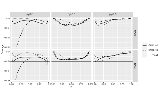
Figure 2: Expected coverage, as a function of $p_{1},p_{2}$, of three 95 % confidence intervals for $N=20$ and $N=50$: the .5 transformed logit (Tlogit) intervals and the GWD intervals for $\ell=2,3$.

Figure 2 reveals that the true coverage of the GWD confidence interval is larger than the nominal value of 95% for $\ell=2$ for almost all the pairs $(p_{1},p_{2})$ considered. It performs as well as the .5 transformed logit confidiecne interval. For $\ell=3$ the GWD coverage when $p_{2}=0.1$ and $p_{1}<.3$ is well below 95%. This could be expected considering the discussion in Section 3.2. In these cases the GWD prior expectation of $K$, $n_{\bullet\bullet}+1$ is in general much smaller than the true number of units that have not been captured. The Waring $\ell=3$ prior underestimates the uncertainty for the population size $N$.

The next step is to compare the relative lengths of the GWD, with $\ell=2$, and the .5 transformed logit confidence intervals. First samples with $n_{11}$ equal to 0 or 1 are excluded, as not containing much information about population size. For the remaining ${(N+1)\choose 3}$ samples, the relative lengths, e.g. the lengths divided by the population size, of the two 95% confidence intervals under study were evaluated. Figure 3 shows boxplots of the $\ell=2$ GWD and the .5 transformed logit relative lengths, for $N=20,50$. The samples for which the length of at least one of the two confidence intervals are larger than 50 have been discarded.

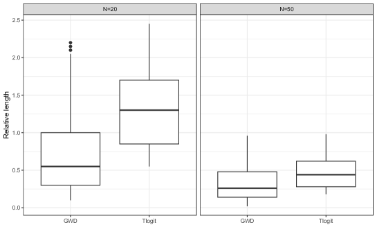
Figure 3: Boxplots for the relative length of the 95% .5 transformed logit (Tlogit) confidence interval and the corresponding GWD, with $\ell=2$, 95% confidence interval. This representation only visualizes the distribution of the relative length when the observed confidence interval length for both methods is less than 50.

In Figure 3 the length of the .5 transformed logit 95% confidence is larger than the corresponding GWD interval with $\ell=2$ for 94.4% of the samples when $N=20$. Indeed the GWD confidence intervals length is less than half that of the .5 transformed logit interval when $N=20$. When $N=50$ the GWD confidence intervals retains its superiority even if the differences are smaller. For larger values of $N$, the $\ell=2$ GWD confidence interval and the .5 transformed logit confidence interval give similar results, as illustrated in the numerical examples of Table 2.

5 Discussion

Generalizations of the methodology presented in this work to experiments with $I>2$ capture occasions is not straightforward. A generalization of Petersen’s model is the class of log-linear models proposed in Fienberg (1972). These models have sufficient statistics for the nuisance parameters and the conditional distribution of the data given those sufficient statistics is sometimes known. For instance, when there are $I=3$ capture occasions, consider the model with an interaction between occasions 2 and 3. The conditional distribution of the data, given the sufficient statistics, is proportional to (5) and the GWD confidence interval applies to this experiment. It suffices to combine capture occasions 2 and 3 in a single capture occasion. In the model of independence between $I>2$ capture occasions, the conditional distribution, given the sufficient statistics for the $I$ capture probabilities, is an extended hypergeometric distribution discussed in Darroch (1958). García-Pelayo (2006) looked at this distribution as one for the population size $N$ given the data. This posterior involves a fairly complex ${{}_{I}}F_{I-1}$ hypergeometric function that does not seem to have been investigated in the statistical literature. Thus, except in some special cases, the methodology presented in this paper does not apply to experiments involving more than two capture occasions and the evaluation of a Bayesian posterior distribution for $N$ needs to be done through a simulation algorithm.

The calculation of most confidence intervals for $N$ in Petersen’s model relies on quantiles of the normal distribution, see Sadinle (2009) and Jensen (1989). GWD confidence intervals are more complex as they involve the GWD distribution. To ease the evaluation of these confidence intervals, R-codes for evaluating the probability mass function (1), the cumulative distribution function and the quantile function of the GWD distribution are provided in the supplementary material. An R-shiny implementing these calculations, ShinywaringCapt, is also available (Rivest and Yauck, 2023).

References

- Castledine (1981) Castledine, B. (1981). “A bayesian analysis of multiple-recapture sampling for a closed population”, Biometrika 68, 197–210.
- Darroch (1958) Darroch, J. N. (1958). “The multiple recapture census I: Estimation of a closed population”, Biometrika 45, 343–359.
- Fienberg (1972) Fienberg, S. E. (1972). “The multiple recapture census for closed populations and incomplete contingency tables”, Biometrika 59, 591–603.
- Fienberg et al. (1999) Fienberg, S. E., Johnson, M. S., and Junker, B. W. (1999). “Classical multilevel and Bayesian approaches to population size estimation using multiple lists”, Journal of the Royal Statistical Society: Series A (Statistics in Society) 162, 383–405.
- García-Pelayo (2006) García-Pelayo, R. (2006). “A Bayesian, combinatorial approach to capture–recapture”, Theoretical population biology 70, 336–351.
- George and Robert (1992) George, E. I. and Robert, C. P. (1992). “Capture—recapture estimation via Gibbs sampling”, Biometrika 79, 677–683.
- Irwin (1963) Irwin, J. O. (1963). “The place of mathematics in medical and biological statistics”, Journal of the Royal Statistical Society 126, 1–41.
- Irwin (1975) Irwin, J. O. (1975). “The generalized Waring distribution. part i”, Journal of the Royal Statistical Society: Series A (General) 138, 18–31.
- Jensen (1989) Jensen, A. L. (1989). “Confidence intervals for nearly unbiased estimators in single-mark and single-recapture experiments”, Biometrics 1233–1237.
- Johnson et al. (2005) Johnson, N. L., Kemp, A. W., and Kotz, S. (2005). Univariate Discrete Distributions. Third Edition, volume 444 (John Wiley & Sons).
- Lecren (1965) Lecren, E. D. (1965). “A note on the history of mark-recapture population estimates”, Journal of Animal Ecology 34, 453–454.
- Lyles et al. (2021) Lyles, R. H., Wilkinson, A. L., Williamson, J. M., Chen, J., Taylor, A. W., Jambai, A., Jalloh, M., and Kaiser, R. (2021). “Alternative capture-recapture point and interval estimators based on two surveillance streams”, in Modern Statistical Methods for Health Research, 43–81 (Springer).
- Rivest and Yauck (2023) Rivest, L.-P. and Yauck, M. (2023). “Shiny: The GWD distribution for capture-recapture”, URL https://stat-appli.shinyapps.io/ShinywaringCapt/.
- Sadinle (2009) Sadinle, M. (2009). “Transformed logit confidence intervals for small populations in single capture–recapture estimation”, Communications in Statistics-Simulation and Computation 38, 1909–1924.
- Seber (1986) Seber, G. A. (1986). “A review of estimating animal abundance”, Biometrics 267–292.
- Seber and Schofield (2019) Seber, G. A. and Schofield, M. R. (2019). “A brief history of capture–recapture”, Capture-Recapture: Parameter Estimation for Open Animal Populations 1–11.
- Seber (1982) Seber, G. A. F. (1982). The Estimation of Animal Abundance and Related Parameters, 2nd edition (Macmillan, New York).
- Webster and Kemp (2013) Webster, A. J. and Kemp, R. (2013). “Estimating omissions from searches”, The American Statistician 67, 82–89.
- Xekalaki (1983) Xekalaki, E. (1983). “The univariate generalized waring distribution in relation to accident theory: proneness, spells or contagion?”, Biometrics 887–895.
- Yule (1925) Yule, G. U. (1925). “Ii.—a mathematical theory of evolution, based on the conclusions of dr. JC Willis”, Philosophical transactions of the Royal Society of London. Series B, containing papers of a biological character 213, 21–87.