1 Experimental setup

1.1 Lock-in detection

To minimize measurement noise, the experiment uses lock-in detection to measure the signal from the balanced photodetector. Ideally, the balanced photodetector output yields $0\text{\,}\mathrm{V}$ in the absence of the THz-pulse. However, drifts can occur due to alignment imperfections or changes caused by thermal effects or by scanning the delay with the Dazzler or mechanical delay stage. To remove these drifts, the THz-pulses are chopped at half the laser repetition rate. Consequently, the balanced photodetector measures periodically one probe pulse with the THz-field and one without it. Since drifts are present in both pulses, it results in a $1\text{\,}\mathrm{k}\mathrm{H}\mathrm{z}$ signal. However, the information about the THz-field strength is present in only one probe pulse yielding a signal at $500\text{\,}\mathrm{H}\mathrm{z}$. By demodulating the signal of the balanced photodetector with a reference signal at $500\text{\,}\mathrm{H}\mathrm{z}$ in a lock-in amplifier, the resulting signal is free from systematic noise and possesses only information about the THz-field.

1.2 Synchronization

Various trigger signals are present in the experimental setup to synchronize the different devices and to ensure accurate data acquisition. Fig. 1 provides a layout of the different trigger signals. The front-end generates a trigger signal at a frequency of $1\text{\,}\mathrm{k}\mathrm{H}\mathrm{z}$ (red) corresponding to the outgoing optical pulse train. This signal triggers both the chopper and the Dazzler. To block every other optical pulse, the chopper uses the first subharmonic of this trigger signal with a frequency of $500\text{\,}\mathrm{H}\mathrm{z}$. This chopping frequency is further used as the demodulation frequency of the lock-in amplifier (green). The Dazzler utilizes the trigger of the Legend to trigger an RF-pulse that drives an acoustic wave in the crystal-unit. A control signal is then sent to the electronic control-board via the ”GATE”-output S1 of the Dazzler (blue, at $1\text{\,}\mathrm{k}\mathrm{H}\mathrm{z}$) for every launched RF-pulse, even if the Dazzler is running but not controlled by the computer.

When a measurement is started by the computer, the information about the acoustic pulses launched within the experiment is send via a USB connection to the Dazzler. The ”PATTERN-GATE” output of the Dazzler becomes high before the first acoustic wave of the sequence is launched, indicating that the Dazzler is running a user-defined sequence controlled by the computer. This output signal remains high until the sequence is over. To ensure that the lock-in signal is sampled only when the user-defined sequence is played and when a pulse passes through the chopper, an electronic control board is used. The board consists of an AND gate and a D-flip-flop. The AND gate combines the ”GATE” and ”PATTERN-GATE” outputs of the Dazzler resulting in a $1\text{\,}\mathrm{k}\mathrm{H}\mathrm{z}$ trigger signal whenever a user-defined sequence is played from the computer. If no user-defined sequence is playing, the AND gate outputs a low signal. In the presence of a sequence, the frequency of the $1\text{\,}\mathrm{k}\mathrm{H}\mathrm{z}$ trigger signal after the AND gate is divided by two using a D-flip-flop to sample only the lock-in amplifier signal of pulses which are passing through the chopper. The signal leaving the electronic board is triggering the data acquisition of the lock-in amplifier.

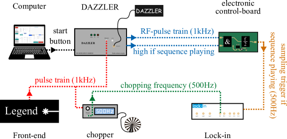
Figure 1: Path of trigger signals required for synchronization and data acquisition

Due to the lack of synchronization between the chopper and the Dazzler in the setup described above, the Dazzler is unable to determine if a pulse is blocked or transmitted by the chopper during the start of a sequence. As a result, in every second measurement in average, the electronic control board produces an incorrect trigger signal sampling the lock-in amplifier when a pulse is blocked by the chopper. In this case, the measurement must be discarded.

1.3 Rapid field measurements

To minimize measurement time, the Dazzler rapidly scans in a shot-to-shot manner, producing the same time delay for a pair of two consecutive probe pulses. Following one pair of probe pulses, a next pair of probe pulses experiences a new delay. As the beam generating the THz-pulse is chopped at half the repetition frequency, each pair of probe pulses coincides with one generated THz-pulse and one blocked pulse. Therefore, for every time-delay within a scan, one probe pulse probes the THz-pulse while the other one serves as a reference. By measuring the probe pulses via a lock-in amplifier, systematic noise present in both probe pulses of a pair is eliminated, leaving only the THz-signal.

For large step sizes or random scanning, the measured signal amplitude can jump from zero to the peak value of the THz-pulse. Hence, the probe pulses have to resolve this and it must be captured with the detection electronics. The UHFLI lock-in amplifier from Zurich Instruments can follow such a jump when using the boxcar averager functionality while reducing noise due to the signals low duty-cycle. Here, the temporal moving average (boxcar) ensures a pure signal of the last data point without any residual contribution by prior data due to the exponential filter function used in traditional lock-in amplifiers.

2 Reconstruction strategy

2.1 Mathematical Description of Compressed Sensing

Compressed Sensing is a technique where an analog signal $s(t)$ is sampled with a low number of $M$ sampling points resulting in the measured $M\times 1$ discrete signal $y[t]$. As it is not feasible to mathematically describe sampling an analog signal $s(t)$, an oversampled $N\times 1$ digital signal $s[t]$ with $N>>M$ sampling points represents the original signal. Sampling this signal can then be described with the $M\times N$ sensing matrix $\Phi$

$$y[t]=\Phi s[t].$$ (1)

As an example, the sensing matrix $\Phi$ can be the spike basis possessing the columns $\phi_{i}[t]=\delta[t-i]$ in the sensing matrix [1].

Compressed Sensing requires the signal $s[t]$ to be sparse in some orthonormal basis. The original signal $s[t]$ can be expressed in this basis with a $N\times N$ basis matrix $\Psi$ and a $N\times 1$ amplitude vector $\vec{c}$

$$s[t]=\Psi\vec{c}.$$ (2)

One example for an orthonormal basis is the Fourier-basis with the discrete-Fourier-transform (DFT) matrix as the basis matrix $\Psi$.

The original signal can be regained by solving the equation

$$y[t]=\Phi\Psi\vec{c}$$ (3)

for the vector $\vec{c}$. Since this system is undetermined, the unique solution can be found by solving for the minimum $l_{0}$ norm of $\vec{c}$. However, to obtain the minimum $l_{0}$ norm, all possible solutions need to be tried out making the problem not feasible to compute.

Hence, in Compressed Sensing one usually solves the optimization problem [2, 1]

$$\text{min }||\vec{c}||_{1}\text{ subject to }y[t]=\Phi\Psi\vec{c},$$ (4)

where $||\vec{c}||_{1}=\sum_{i}|c_{i}|$ is the $l_{1}$ norm. The solution of equation 3 has the minimum $l_{1}$ norm of $\vec{c}$.

The necessary condition to regain $s[t]$ from the measured signal $y[t]$ is that the reconstruction matrix $\Theta=\Phi\Psi$ needs to obey the restricted isometry property (RIP). As this condition is hard to check, the incoherence between the matrices $\Phi$ and $\Psi$ can be used as an indication for a stable and faithful reconstruction. The coherence between the two matrices is defined as [2, 1]

$$\mu(\Phi,\Psi)=\sqrt{N}\max_{i\leq M,j\leq N}|\langle\phi_{i},\psi_{j}\rangle|,$$ (5)

measuring the largest correlation between any of the elements in the two matrices.

The coherence values that can yield values in the range from $1$ to $\sqrt{N}$, with 1 being the value of maximum incoherence. A higher degree of incoherence, which translates to lower coherence values, increases the likelihood of accurately reconstructing the signal $s[t]$. In certain instances, the incoherence value is calculable. For instance, the spike basis possesses a maximum incoherence of $\mu=1$ with the Fourier-basis, while the noiselet basis has a coherence value of $\mu=\sqrt{2}$ with the wavelet basis. For a fixed basis with matrix $\Psi$ of unknown coherence to any sensing matrix $\Phi$, the sensing matrix can be chosen to be a random, orthonormal matrix. This results in a high probability of having a low coherence value with the fixed matrix $\Psi$ [2, 1].

2.2 Convex Compressed Sensing Reconstruction

Equation 4 can be understood as a convex optimization problem which can be solved by linear programming algorithms. Since the problem as stated in equation 4 is not considering noise, the so called basis pursuit algorithm can only reconstruct a stable, faithful solution for noise-free measurements. For noisy measurements, it is not optimal to solve equation 3 exactly. Therefore, a relaxed problem needs to be formulated [2]. Two convex approaches capable of dealing with noisy measurements are investigated for compressed sensing. The first algorithm is called basis pursuit denoising optimizing the problem [3]

$$\min||\vec{c}||_{1}\text{ subject to }\frac{1}{2}\left|\left|\Phi\Psi\vec{c}-y[t]\right|\right|_{2}^{2}\leq\sigma,$$ (6)

where $\sigma$ is a parameter chosen according to the magnitude of noise in the measurement. The second algorithm is solving the so called Lasso problem given as [3]

$$\min\frac{1}{2}\left|\left|\Phi\Psi\vec{c}-y[t]\right|\right|_{2}^{2}\text{ subject to }||\vec{c}||_{1}\leq\tau,$$ (7)

where the parameter $\tau$ is the regularization parameter of the problem.

Open source Lasso and basis-pursuit denoise algorithms are investigated [4, 3]. For the Lasso as well as the basis-pursuit problem, the value of $\tau$, respectively $\sigma$ needs to be determined empirically. For that, one randomly sampled trace with $N=88$ sampling points of the UHLFI measurement set is used for the determination of $\tau$ and $\sigma$. This explicit measurement is taken, since the number of sampling points correspond to the measurement with the linear sampling scheme with $\Delta t=$341\text{\,}\mathrm{f}\mathrm{s}$$. This step size yields a Nyquist-frequency of $f_{\text{Nyquist}}\approx$1.5\text{\,}\mathrm{T}\mathrm{H}\mathrm{z}$$ positioned in the middle of the absorption spectrum of water vapor. Therefore, this measurement correlates to the border in which compressed sensing could outperform the Fourier-transformation of a traditional linear sampling scheme.

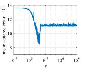
(a) Lasso

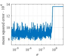
(b) Basis-pursuit denoise

Figure 2: Mean squared error of reconstructed traces from a randomly sampled measurement with $N=88$ sampling points with respect to an oversampled reference trace. The figure compares the mean squared error for the reconstruction performed by the Lasso (a) and the basis-pursuit denoise (b) algorithm for different values of $\tau$, respectively $\sigma$.

The data is fed to the Lasso as well as the basis-pursuit denoise algorithm for different values of $\tau$ and $\sigma$, respectively [5]. For the respective reconstructed traces, the mean squared error to a oversampled reference trace is calculated. The results are depicted in Fig. 2. Both algorithms exhibit a similar minimal value of the mean squared error. However, the Lasso algorithm possesses a distinct global minimum at $\tau\approx 70$, whereas the basis-pursuit denoise algorithm shows a constant minimum value for $\sigma<10^{-1}$. Since it is not always possible to find a reference for arbitrary measurements to optimize the value of $\tau$, the basis pursuit algorithm fits better as a compressed sensing algorithm for accelerating time domain spectroscopy. Consequently, solely the basis pursuit algorithm with a fixed value of $\sigma=10^{-6}$ is investigated.

2.3 StOMP

A reconstruction program consisting of the three algorithms StOMP, TRF and iFFT was developed for evaluating the measured data [The code will be publicly available upon acceptance for publication]. The code aims for fast data processing, minimum human intervention and control characteristics of result. Stagewise Orthogonal Matching Pursuit is a greedy algorithm developed in 2012 which is popular due to the low level of computational complexity resulting in fast data processing [6].

The developed implementation of the iterative algorithm StOMP is shown in Algorithm 1. In each iteration $s$, the different entries of the sparse domain $\vec{c}$ for a residual signal $r_{s}$ are weighted via the matched filter $\kappa_{s}=\Theta^{\text{T}}r_{s}$ (In case of the first iteration: $r_{0}=y$). The result $\kappa_{s}$ scales the presence of the different entries of $\vec{c}$ in the signal $r_{s}$. The most prominent entries are selected via a threshold $\tau_{s}$ yielding a set of outliers $J_{s}=\{j:|\kappa_{s}(j)|>\tau_{s}\}$. The threshold $\tau_{s}=t_{s}\cdot\sigma_{s}$ is constructed by a threshold parameter $t_{s}$ and the formal noise level of the residual $r_{s}$ given by

$$\sigma_{s}=\frac{||r_{s}||_{2}}{\sqrt{\text{dimension}(r_{s})}}.$$ (8)

The entries in this set are merged with all the previous found outliers given in the set $I_{s-1}$ updating the total set of detected outliers $I_{s}=I_{s-1}\cup J_{s}$. The projection of the measured data on the detected outliers $I_{s}$ yields the result for this iteration

$$\vec{c_{s}}=\left(\Theta^{\text{T}}_{I_{s}}\Theta_{I_{s}}\right)^{-1}\Theta^{\text{T}}_{I_{s}}y.$$ (9)

Here, $\Theta_{I_{s}}$ indicates the $M\times|I_{s}|$ matrix which is constructed of $\Theta$ by choosing only the columns according to the index set $I_{s}$. With that, the result $\vec{c_{s}}$ possesses nonzero values for the dominant entries in $I_{s}$ weighted by the projection of the measured signal $y$. If a certain exit condition is fulfilled, $c_{s}$ yields the final result of the algorithm. If the exit condition is not yet fulfilled, the residual for the next iteration is updated by $r_{s+1}=y-\Theta\vec{c_{s}}$. Consequently, the residual of the next iteration $r_{s+1}$ contains the remaining signal contributions which have not been yet detected.

The value of the threshold parameter $t_{s}$ to achieve an optimal reconstruction depends on the input signal $y$ and is varying significantly between different measurements. Hence, we developed an automatic thresholding approach based on the Inter-Quartile Range (IQR) method for outlier detection [7]. The IQR indicates the midspread of a dataset and is defined as the difference of the third and first quartile $IQR=Q_{3}-Q_{1}$. The first and third quartile are hereby defined as the mean of the lower and upper half of a statistical distribution, respectively. In the developed algorithm, $t_{s}$ is calculated by the formula

$$t_{s}=\frac{Q_{3}+\gamma\cdot IQR}{\sigma_{s}},$$ (10)

where $\gamma$ is a set filter value dictating the sensitivity to reconstruct less dominant entries of $\vec{c}$ in the measured signal.

The discussed reconstructions in this work were computed with a filter value of $\gamma=1.8$. The developed algorithm applies the threshold only to entries $\vec{c_{s}}$ within in a set of given boundary conditions. In the case of the presented measurements, only entries corresponding to frequencies within the spectrum of the excitation pulse $f\leq$2.5\text{\,}\mathrm{T}\mathrm{H}\mathrm{z}$$ are considered. To improve the robustness of the algorithm, a range of sparsity for the reconstructed signal is defined. In case the set of detected outliers $I_{s}$ contains a number of entries below the minimum allowed sparsity, the algorithm fills this set by the most prominent entries of $\vec{c_{s}}$ according to the matched filter until the set possesses the minimum allowed sparsity. In case the set $I_{s}$ is above the maximum allowed sparsity, the algorithm stops and returns the solution of the current iteration $c_{s}$.

As StOMP is indifferent towards amplitude optimization, a Nonlinear Least Squares (NLS) solver was included in the reconstruction algorithm. The “Nonlinear Least Squares” solver is a wrapper for scipy.optimize.curve_fit which is a wrapper for scipy.optimize.least_squares, the used algorithm is “Trust Region Reflective”. It has been chosen because it is well suited for large sparse optimization problems. We choose to use scipy.optimize.curve_fit instead of scipy.optimize.least_squares because its user-friendliness compared to other optimization methods in python. Due to the fact that NLS only optimizes the result of StOMP and does not “’add’ any frequency to the optimized result, only a few iterations are needed. NLS tries to minimize the error between the reconstruction and the measurement in time domain. Therefore, it is capable of changing/readjusting all nonzero values of the reconstruction in frequency domain.

Algorithm 1 Our Implementation of StOMP (”IQR”-Mode)

compressed measurement: $y$, reconstruction matrix: $\Theta$, maximum stages: $max_{stages}$, filter value: $\gamma$, boundary condition: $b$, minimum sparsity ratio: $min_{sparsity}$, maximum sparsity ratio: $max_{sparsity}$

for $s=1,s\leq max_{stages}:i\,+=1$ do

     $\kappa_{s}=\Theta^{T}r_{s}$ $\triangleright$ Matched Filter

     if $s==1$ or $J_{s-1}==\{\,\}$ then

         $t_{s}=\frac{\textsc{treshold}(\kappa_{s}\,,b\,,\gamma)}{\sigma_{s}}\text{ for }\kappa_{s}\in\{b\}$

     else

         $t_{s}=t_{s-1}$

     end if

     $J_{s}=\{j:\lvert\kappa_{s}(j)\rvert>t_{s}\sigma_{s}\}$ $\triangleright$ Hard Thresholding

     if sparsity ratio($\kappa_{s}$, $I_{s-1}$, $J_{s}$) $<\;min_{sparsity}$  then

         while sparsity ratio($\kappa_{s}$, $I_{s-1}$, $J_{s}$) $<\;min_{sparsity}$  do $\triangleright$ If sparsity to low increase it until it is ok

              $J_{s}\cup\{j:\lvert\kappa_{s}(j)\rvert\geq\lvert\kappa_{s}(n)\rvert\,\forall\,n\}$

         end while

     end if

     $I_{s}=I_{s-1}\cup J_{s}$ $\triangleright$ Updating Index Set

     $(c_{s})_{I_{s}}=(\Theta^{T}_{I_{s}}\Theta_{I_{s}})^{-1}\Theta^{T}_{I_{s}}y$ $\triangleright$ Projection

     $r_{s+1}=y-\Theta_{I_{s}}c_{s}$ $\triangleright$ Updating residual

     if sparsity ratio($\kappa_{s}$, $I_{s-1}$, $J_{s}$) $\geq\;max_{sparsity}$  then $\triangleright$ If sparsity ok or to hight stop

         end for

     end if

end for

return $c_{s}$

Algorithm 2 sparsity ratio

function sparsity ratio($\kappa_{s}$, $I_{s-1}$, $J_{s}$)

     return $\frac{\mid I_{s-1}\mid+\mid J_{s}\mid}{dim(\kappa_{s})}$

end function

Algorithm 3 Threshold $t_{\text{IQR}}$ Calculation

function threshold($\kappa_{s}$, $b$, $\gamma$)

     $C=\{\mid\kappa_{s}(j)\mid:j\in b\}$ $\triangleright$ absolut values with respect to index boundaries

     $Q_{1}=P_{25}^{\hskip 1.39998ptC}$ $\triangleright$ Percentil $0\text{ to }25\%$

     $Q_{3}=P_{75}^{{\hskip 1.39998ptC}}$ $\triangleright$ Percentil $75\text{ to }100\%$

     $IQR=Q_{3}-Q_{1}$ $\triangleright$ Interquartil range calculation

     $t_{\text{IQR}}=Q_{3}+\gamma\cdot IQR$ $\triangleright$ threshold calculation

     return $t_{\text{IQR}}$

end function

3 Reconstruction details

3.1 Basis and measurement matrix

Compressed sensing algorithms require a measurement matrix $\Phi$ as well as a basis matrix $\Psi$. In this work, the discrete-Fourier-transformation (DFT) is used as the basis matrix $\Psi$. Hence, the entries $\vec{c}$ correspond to the frequency spectrum of the measured signal.

The size of the basis and the corresponding matrix $\Psi$ is determined by the length of the time vector for the reconstructed signal. The time vector and the correlating measurement matrix can be chosen arbitrarily. In the present work, the minimum and maximum of the time vector is bound to the temporal window of the molecular response. This allows to compare the Fourier-transformation of the reconstruction to the one of the linear sampled data laying within this window with equal spectral resolution. The step size of the time vector for the reconstruction is upper bounded by the Nyquist criteria of the signal. By decreasing the step size, the quality of the reconstruction improves since differences between time points of the reconstruction and the random time points of the measurement are decreasing. However, decreasing the step size is increasing the size of the matrices and hence the computation time. In this work, we use a moderate step size of $\Delta t=$75\text{\,}\mathrm{f}\mathrm{s}$$.

In the case of the basis pursuit denoise algorithm, a boundary matrix $\Sigma$ able to set boundary conditions is added to the basis matrix $\Psi_{\text{BPD}}=\Psi\Sigma$. $\Sigma$ allows to define a frequency range for non-zero values while keeping the DFT matrix large. We selected a frequency range from $0$ up to $2.5\text{\,}\mathrm{T}\mathrm{H}\mathrm{z}$ corresponding to the spectrum of the excitation pulse. A large DFT matrix is favorable in BPD, since this corresponds to a fine time step of the reconstructed time signal. For finer time steps, the error calculation $||\Phi\Psi\vec{c}-y[t]||$ is more accurate, as the time points of the reconstructions are closer to the random time points of the measured signal. The boundary matrix transports the vector $\vec{c}$ with entries laying in the defined spectral region into the columns of a large fft matrix corresponding to the respective frequencies of $\vec{c}$.

3.2 BPD reconstruction of measurements with different lock-in amplifier

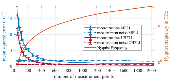
Figure 3: Mean and indicated standard deviation of the mean squared error of reconstructed traces for three different sets of measurements. The mean squared error is calculated with respect to an average of ten oversampled reference traces of the respective measurement set. In the figure, the reference shows the mean squared error of the linear sampled data with respective number of sampling points to the same reference trace.

The quality of reconstructed traces via BPD for two sets of measurements performed with two different lock-in amplifiers (UHLFI and MFLI from Zurich Instruments) are compared. The lock-in amplifier UHFLI is using the boxcar averager option to reduce noise due to the low duty cycle of the signal of the balanced photo diodes. The lock-in amplifier MFLI acquires data without a boxcar averager option. To speed up settling of the MFLI’s low-pass filter to avoid unwanted contribution due to the exponential filter, the time constant is lowered. To attenuate signal contributions of DC offsets, non-linearities and signal components situated at twice the demodulation frequency, a sinc-filter is applied. The combination of the low time constant with the sinc-filter results in higher measurement noise compared to the detection with the boxcar filter. Consequently, we are able to compare the quality of reconstruction of measurements with two different noise levels. For a quantitative comparison, the mean squared error of the reconstructed traces for the random sampled measurements is calculated with respect to the average of the ten linear sampled traces with the lowest step size for the respective set of measurements. The mean as well as the standard deviation for the mean squared error of the ten repetitions for different number of sampling points are shown in Fig. 3. As a measure for the measurement noise, the mean squared error of the linear sampled measurements is depicted for the different number of sampling points. The MFLI measurement exhibits measurement noise which is by a factor of three higher compared to the UHFLI measurement. For measurements possessing a large number of sampling points, the BPD reconstruction is below the noise level for both set of measurements. However, the reconstructions of the MFLI measurement show a bigger noise rejection with respect to the noise level compared to the UHFLI measurement. This shows the potential of compressed sensing in improving the signal quality of noisy measurements.

3.3 BPD reconstruction quality

The reconstruction quality of linearly sampled and randomly sampled measurement are compared in Fig. 4 and 5. The probability to reconstruct absorption peaks via BPD for a randomly sampled waveform with $N=46$ is shown in Fig 6.

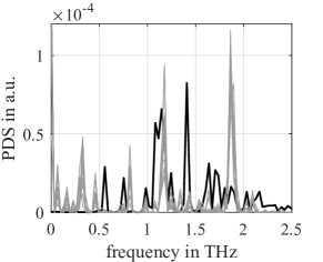
(a)

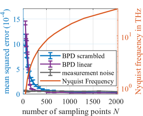
(b)

Figure 4: a) Power density spectrum (PDS) of the reconstruction of ten linear sampled measurements with $N=47$ (gray) and the PDS of an oversampled reference trace (black). b) Mean squared error of the BPD reconstruction of linear (purple) and scrambled (blue) measurements with respect to an oversampled reference for different number of sampling points. The measurement noise (grey) is given by the mean squared error of the raw linear sampled measurements with respect to the oversampled reference. The Nyquist frequency for the corresponding number of sampling points is given in orange.

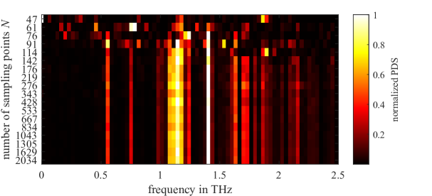
Figure 5: Averaged Power density spectra (PDS) for the BPD reconstruction of ten linear sampled measurements for different number of sampling points.

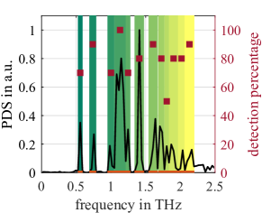
(a) $\text{threshold}=0.005$

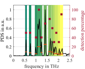
(b) $\text{threshold}=\frac{\text{peak value of reference}}{4}$

Figure 6: Probability to reconstruct absorption peaks via BPD for a randomly sampled waveform with $N=46$ sampling points. An absorption peak is declared as detected if the reconstruction possesses a value greater than the given threshold (orange) in the area of the respective absorption. The threshold is given as the noise level of the reference (black) $\text{threshold}=0.005$ in a) and as a quarter of the respective absorption peak value of the reference in b).

References

- [1] Emmanuel J. Candes and Michael B. Wakin “An Introduction To Compressive Sampling” In IEEE Signal Processing Magazine 25.2, 2008, pp. 21–30 DOI: 10.1109/MSP.2007.914731
- [2] Meenu Rani, S.. Dhok and R.. Deshmukh “A Systematic Review of Compressive Sensing: Concepts, Implementations and Applications” In IEEE Access 6, 2018, pp. 4875–4894 DOI: 10.1109/ACCESS.2018.2793851
- [3] E. Berg and M.. Friedlander “Probing the Pareto frontier for basis pursuit solutions” In SIAM Journal on Scientific Computing 31.2, 2008, pp. 890–912 DOI: 10.1137/080714488
- [4] E. Berg and M.. Friedlander “SPGL1: A solver for large-scale sparse reconstruction” https://friedlander.io/spgl1, 2019
- [5] Kilian Scheffter “Accelerating Terahertz Field-Resolved Spectroscopy”, 2022
- [6] David L. Donoho, Yaakov Tsaig, Iddo Drori and Jean-Luc Starck “Sparse Solution of Underdetermined Systems of Linear Equations by Stagewise Orthogonal Matching Pursuit” In IEEE Transactions on Information Theory 58.2, 2012, pp. 1094–1121 DOI: 10.1109/TIT.2011.2173241
- [7] H.. Vinutha, B. Poornima and B.. Sagar “Detection of Outliers Using Interquartile Range Technique from Intrusion Dataset” In Information and Decision Sciences Singapore: Springer Singapore, 2018, pp. 511–518