The impact of supernova feedback on the mass–metallicity relations

Abstract

Metallicity is a fundamental physical property that strongly constrains galaxy formation and evolution. The formation of stars in galaxies is suppressed by the energy released from supernova explosions and can be enhanced by metal production. In order to understand the impact of this supernova feedback, we compare four different feedback methods, ejecting energy in thermal, kinetic, stochastic and mechanical forms, into our self-consistent cosmological chemodynamical simulations. To minimise other uncertainties, we use the latest nucleosynthesis yields that can reproduce the observed elemental abundances of stars in the Milky Way. For each method, we predict the evolution of stellar and gas-phase metallicities as a function of galaxy mass, i.e., the mass–metallicity relations. We then find that the mechanical feedback can give the best match to a number of observations up to redshift $z\sim 3$, although the predicted gas-phase metallicities seem to be higher than observed at $z>\kern-11.99998pt\lower 4.73611pt\hbox{$\sim$}~{}1$. The feedback modelling can be further constrained by the metallicities in distant galaxies with the James Web Space Telescope and those of a large sample with ongoing and future spectroscopic surveys.

1 Introduction

The evolution of elemental abundances in the universe across cosmic time is essential to understand the formation and evolution of galaxies (e.g., Kobayashi & Taylor, 2023, for a review). While the evolution of dark matter in the standard $\Lambda$ cold dark matter ($\Lambda$-CDM) cosmology is well understood, one of today’s greatest challenges is understanding the evolution of baryonic matter from primordial elements produced in the Big Bang nucleosynthesis to elements heavier than helium produced in stars. Metals are observed in the local to the distant galaxies. The abundances of metals in galaxies give information about the star formation rate (SFR), gas outflows, and inflow during the galaxies’ histories. The study of metallicity also provides crucial information about the exchange of metals between stars, the cold interstellar gas, and the diffuse surrounding gas.

Understanding the origin and behaviour of elements is subject to several studies. Chemical elements are produced during different astronomical events. Hydrogen and helium form through the Big Bang nucleosynthesis, while carbon and heavier elements form in stellar nucleosynthesis from core-collapse supernovae (SNe), asymptotic giant branch (AGB) stars, thermonuclear explosions observed as Type Ia supernovae (SNe Ia), and neutron star mergers observed as kilonovae (Kobayashi et al., 2020b). Metals are produced in stars and are ejected into the interstellar medium (ISM), circumgalactic medium (CGM), and the intergalactic medium (IGM) (e.g., Péroux & Howk, 2020). This ejection happens through losing the outer gaseous envelopes of old/dying stars or the explosion of massive stars as supernovae (with initial masses $>\kern-11.99998pt\lower 4.73611pt\hbox{$\sim$}~{}10M_{\odot}$). The energy released through stellar winds and supernovae explosions is known as stellar feedback (e.g., Larson, 1974). Feedback can efficiently suppress star formation by heating and evaporating dense, star-forming clouds, generating turbulent supersonic shocks, and generating outflows that eject gas from the galaxy. At low halo masses, the dominant feedback is from massive stars (stellar winds, supernova explosions, photoionization, and radiation pressure). Whereas at higher masses, active galactic nucleus (AGN) feedback dominates (e.g., Silk 2013; Taylor & Kobayashi 2015). Different feedback methods are used in different cosmological simulations, such as thermal feedback (e.g., Katz 1992) kinetic feedback (Navarro & White, 1993), stochastic feedback (Dalla Vecchia & Schaye, 2012), and mechanical feedback (Hopkins et al., 2018; Smith et al., 2018). In this paper we investigate the impact of supernova feedback on the metallicities of galaxies using the same stellar yields in our cosmological simulations.

Cosmological simulations consider two different processes for the evolution of galaxies over cosmic time: (1) The hierarchical growth of dark-matter structures on timescales proportional to redshift (Press & Schechter, 1974). (2) The baryonic physics on timescales that are impacted by the processes such as radiative cooling, star formation, and feedback (White & Rees, 1978). The simulation of galaxy formation and evolution remains a significant challenge as it extends from large-scale structures along dark matter filaments to star formation scales. Assumptions and approximations are therefore necessary and depend on the scale we want to resolve. For instance, the semi-analytic models (SAMs) (White & Frenk, 1991) compute the baryonic physics separately from the dark matter. SAMs treat each galaxy as an unresolved object and provide a statistical sample of galaxies. On the other hand, hydrodynamical simulations model the hydrodynamics and gravitational laws and can simulate the baryonic physics simultaneously with the dark matter self-consistently. These simulations can also predict the internal structure of galaxies (i.e., kinematics and spatial distributions). However, the results are still limited to a finite resolution. Therefore, all currently available hydrodynamical models implement analytical laws to attempt to capture the effects of the above mentioned sub-galactic processes on a galaxy scale.

Several hydrodynamical simulations are used to predict the evolution in galaxies, with very different input physics in each simulation. For example, the EAGLE simulations (Schaye et al., 2015) use stochastic feedback (Dalla Vecchia & Schaye, 2012). Illustris uses bipolar winds, IllustrisTNG (Pillepich et al., 2018) uses isotropic, kinetic (wind) feedback from (Springel & Hernquist, 2003), SIMBA (Davé et al., 2019) uses stellar kinetic feedback with decoupled wind particles, HORIZON-AGN (Dubois et al., 2016) uses thermal energy injection to model stellar feedback. In this paper, we use our own chemodynamical code (Taylor & Kobayashi, 2014) based on the GADGET hydrodynamical code (Springel et al., 2001a, 2005) to systematically investigate the effects of supernova feedback on the chemical evolution of galaxies.

Measuring metallicity from observed spectra of galaxies is subject to many previous studies, is an ongoing effort, and is available for stellar populations (e.g., Worthey et al., 1992; Conroy, 2013) and the ISM (e.g., Maiolino & Mannucci, 2019; Kewley & Ellison, 2008). The stellar mass–metallicity relation (MZR) was first discovered in local elliptical galaxies by studying the colour-magnitude diagram (McClure & van den Bergh, 1968). The relation for the ISM was first observed in a small sample of nearby star-forming galaxies by Lequeux et al. (1979). Later on, using the Sloan Digital Sky Survey (SDSS), several authors derived a clearer MZR for stars (e.g., Gallazzi et al. 2006; Zahid et al. 2017) and the ISM (Tremonti et al., 2004; Curti et al., 2020), where galaxy metallicity increases with stellar mass. Various methods are used to infer the metallicity of the gaseous phase. The main ones are different calibrations with the photoionization models (Kewley & Ellison, 2008), strong line calibration (Curti et al., 2020), and direct method based on electron temperature (Curti et al., 2023).

In this paper, we implement and compare four models of stellar feedback in our cosmological simulations. The physical processes included in our simulation are described in section 2. The results of the different feedback models on the MZR are presented in section 3. Comparing with the observed MZRs, we discuss our results and give our perspectives in section 4.

2 Model

Our simulation code is based on the "GAlaxies with Dark matter and Gas intEracT 3" code known as GADGET-3 (Springel et al., 2005). It uses TreeSPH (Hernquist & Katz, 1989), which combines the smoothed particle hydrodynamics (SPH) (Lucy, 1977; Gingold & Monaghan, 1977) to follow the gas dynamics, with the hierarchical tree algorithm to compute the N-body gravitational interactions. The long-range force is calculated with the PM-algorithm using Fourier techniques. We use an improved version of the code that contains several physical processes related to galaxy formation and evolution, such as radiative cooling, star formation, supernovae feedback (Kobayashi et al., 2007), and black hole (BH) physics (Taylor & Kobayashi, 2014).

2.1 Baryonic Physics

Gravitational instability physics (i.e. dark matter structures) is an important starting point in galaxy formation models. However, one of today’s greatest challenges in cosmological simulations is implementing the baryonic astrophysical processes that describe the galaxy population. The key difference between dark and baryonic matter is that the latter can dissipate energy through radiative processes. In what follows, we discuss the main processes involved in galaxy formation.
Radiative Cooling: Radiative cooling is a process that allows a space object to lose heat by thermal radiation. It uses the cooling function $\Lambda(T)$, which expresses gas cooling by thermal radiation. This function assumes that the gas is optically thin (i.e. an emitted photon can typically leave the cloud). An example of a set of cooling curves is given by Sutherland & Dopita (1993) where $\Lambda(T)$ has multiple peaks and valleys because the emission mechanisms are most efficient at specific temperatures. For instance, it is characterised by a big bump at low temperature produced by line radiation and a tail at high temperature (above $10^{7}$K) produced by Bremsstrahlung. We also include Compton heating. In this work, we use the same metallicity-dependent cooling function implemented by Kobayashi (2004), which is computed with the MAPPINGS-III software (Sutherland & Dopita, 1993).
Star Formation: In galaxy simulations the formation of star particles is only allowed in a gas that obeys certain conditions, stars are formed in cool dense gas. As in Kobayashi et al. (2007), we use the star formation criteria used in Katz (1992), which are: (1) Star formation is only allowed in convergent flows, (2) Star formation is only allowed in regions where the cooling time is less than the dynamical time (rapid cooling), and (3) The gas has to be locally Jeans unstable.
Stellar Feedback: It is observed that stars represent less than 10$\%$ of the baryonic matter in the observable Universe (Madau & Dickinson, 2014). However, according to the predictions of the cosmic microwave background (CMB) models, all the gas has already cooled and formed stars by today. This problem was recognised by the earliest models of galaxy formation (White & Rees 1978, Dekel & Silk 1986) where they suggested that this overcooling may be solved by the consideration of the supernova feedback. Supernova energy heats the gas, dispersing out of the galaxy and reducing the galaxy’s baryon fraction, leading to a star formation inefficiency. There are two classes of feedback mechanisms that retard star formation, ejective and preventive feedback. Ejective feedback ejects the gas from the ISM, while preventive feedback stops the gas from accreting into the ISM. On the contrary, dying stars and supernovae eject metals, which enhance cooling and star formation (e.g., Kobayashi et al., 2007). We include these effects self-consitently. More detail is given in Sect. 2.2.
AGN Feedback: In addition to supernova feedback, feedback from AGNs is essential in suppressing star formation in massive galaxies (e.g., Silk, 2013; Taylor & Kobayashi, 2015). In a star-forming galaxy (with cool and dense gas) where the BH is not yet active, part of the gas produces stars, and the other part falls into the BH. After accreting enough gas, the BH becomes active and ejects outflows and radio jets. This mechanism, known as AGN feedback, heats and pushes the gas away, which slows down star formation and stops the BH from growing. No more fuel will cause the BH to deactivate, meaning nothing will heat the gas anymore (for it to expand), so it returns to the initial BH stage. At this stage, the gas can cool again. However, stars only form if the gas is dense enough, which is usually not the case.

As in Taylor & Kobayashi (2014), AGN feedback in our simulation is modelled as (1) BH seed formation: the seed BHs are formed with the first stars, any gas particle with a density higher than the specified critical density and with zero metallicity ($Z=0$) is converted into a BH particle with a seed mass of $1000h^{-1}M_{\odot}$. (2) Growth: The seed BHs grow by accreting gas and by merging with other BHs. (3) AGN feedback: In each timestep, a certain amount of energy is produced by the BH and is distributed in a thermal form to a fixed number of neighbour gas particles.
Chemical Enrichment: In our simulations, a star particle is not a single star but a set of many. We consider a star particle as a simple stellar population (SSP, i.e. stars with the same age and metallicity but different masses) and include a chemical enrichment model that tracks the enrichment of the gas with all elements up to zinc. Oxygen, carbon and iron abundances are mainly produced by core-collapse SNe, AGB stars, and SNe Ia, respectively (Kobayashi et al., 2020b). The initial mass function (IMF) of stars is taken from Kroupa (2008). We compute oxygen abundance for the ISM to compare with observations of metallicities weighted by SFRs. And we use total metals for stellar metallicities weighted by V-band luminosities.

2.2 Stellar feedback

In hydrodynamical simulations, gas particles are affected by nearby star particles locally. We also follow the cooling of the gas particles after the feedback. These are fundamentally different from the loading factor in previous work (e.g., Belfiore et al., 2016; Lian et al., 2018; Lin & Zu, 2023), which is the measure for the average effect of or within the galaxy (see Taylor et al. 2020 for comparison between simulations and observations). In the following, we describe four feedback methods proposed for hydrodynamical simulations.
Thermal feedback: The classical stellar feedback method used in galaxy simulations consists of the distribution of thermal energy from supernova explosions into the surrounding gas (e.g., Katz 1992), namely, to the neighbour particles in a fixed radius or with a fixed number, using a smoothing kernel $W_{j}$.

$$\Delta E=E_{\rm SN}W_{j}$$ (1)

Where $\Delta E$ is the weighted fraction of the supernova energy received by the $j^{\rm th}$ gas particle, and $E_{\rm SN}$ is the total energy ejected by supernovae from an evolving star particle in a given time step. In our simulations, $N_{\mathrm{ngb}}$ nearest neighbour gas particles are selected and receive the supernova energy weighted by the smoothing kernel. Then at each time step, the total ejected energy $E_{\rm SN}$ is divided accordingly to the weighting to heat the gas particles individually.

Our simulations also include hypernova feedback (Kobayashi et al., 2007). Since the energy of hypernovae is more than ten times larger than the supernova energy ($10^{51}$ erg), the temperature increase can be much more significant and can reach $\sim 10^{6}$ K. Once the gas particles are heated to this temperature, they do not cool rapidly due to the low cooling rate. As a result, this reduces the SFR significantly, and the hypernova feedback is expected to be more efficient than supernova-only feedback.
Kinetic feedback: This method consists of implementing outflows where the energy input is partially converted to kinetic energy (Navarro & White, 1993). The thermal energy ejected by each supernova explosion is partially reduced by a parameter $f$ ($0\leq f\leq 1$), representing the fraction of energy distributed as kinetic energy. This model simulates a shocked gas with a kinetic kick of velocity $v$ such as:

$$v=\sqrt{2fE_{\rm SN}\mathrm{W}_{j}/M_{j}}$$ (2)

where $M_{j}$ is the mass of the $j^{\rm th}$ gas particle that receives the energy, and $E_{\rm SN}\mathrm{W}_{j}$ is the weighted fraction of the supernova energy received by the $j^{\rm th}$ gas particle. This velocity is added to the original velocity of neighbour particles isotropically.
Stochastic feedback: This approach was first implemented by Kay et al. (2003) in galaxy simulations, and generalised by Dalla Vecchia & Schaye (2012) to complete the thermal feedback method and efficiently suppress star formation. Thermal feedback may be inefficient because the thermal energy is mostly radiated away before it can be turned into kinetic energy. This may be because the mass of the gas receiving the supernova energy is too large. Without hypernovae the energy emitted by supernovae is not enough to efficiently heat these gas particles; hence the gas temperature remains too low and the cooling time too short. Another reason for the thermal feedback inefficiency may be the lack of resolution: the energy is mainly distributed to a high-density gas because the simulation does not resolve the hot and low-density areas (which remain missing).

The temperature jump of the neighbour gas can be increased by reducing the mass of the heated gas with respect to the star particle. This can be done by reducing the number of heated gas particles or by specifying the temperature jump of the heated gas. The first idea may cause an issue if even one gas particle is too massive. The second way can be done using stochastic feedback, where the probability of the gas particle being heated depends on the star-to-gas mass ratio and the specified temperature jump. For the stochastic feedback, the idea is to select a random number of nearby particles (instead of heating all the neighbour particles as in the thermal feedback model).

We use the same model as in Dalla Vecchia & Schaye (2012) where we define an energy increase $\Delta e$ used to heat the neighbour gas particles.

$$\Delta e=f\frac{E_{\mathrm{SN}}}{N_{\mathrm{ngb}}}$$ (3)

where $E_{\mathrm{SN}}$ is the total supernova energy ejected by an evolving star particle in a given timestep, $N_{\mathrm{ngb}}$ is the number of neighbour gas particles, and $f$ is a parameter which is introduced to hold the probability that each of the $N_{\mathrm{ngb}}$ particles receives an energy increase of $\Delta e$ (i.e., $\Delta e>\frac{E_{\mathrm{SN}}}{N_{\mathrm{ngb}}}$, hence $f>1$). $\Delta e$ is the total energy a single gas particle will receive from the supernovae independently from the distance to the star particle. To determine if a gas particle will receive the energy or not, a random number $0<r<1$ is compared to the condition:

$$r<\frac{E_{\mathrm{SN}}M_{*}}{\Delta e\sum_{j}^{N_{\mathrm{ngb}}}M_{j}}$$ (4)

with $M_{*}$ the mass of the star particle and $M_{j}$ the mass of the $j^{\rm th}$ gas particle receiving the energy. The gas particle receives an energy increase of $\Delta_{e}$ only if this condition is satisfied. Larger $f$ results in a smaller number of gas particles heated with a larger energy $\Delta e$. Note that $M_{j}$ and $M_{*}$ are not constant in our simulations.
Mechanical feedback: Mechanical feedback takes into account the supernova shock wave applied to gas particles. This model uses assumptions depending on the structure of the ISM at small scales and its interaction with the supernova remnants. As the supernova shock wave propagates, it accelerates particles, radiating energy away. There are mainly three phases in the life of a supernova.: i) the free expansion phase, ii) the adiabatic or Taylor-Sedov phase (Taylor, 1950; Sedov, 1959), where the expansion proceeds adiabatically into the surroundings, and radiative losses are negligible. And iii) the radiative or ‘snowplough’ phase, where the gas temperature in the shock wave drops as the cooling function increases and the shock slows until it merges with the surroundings and disappears.

We implement mechanical feedback similar to Hopkins et al. (2014) and Smith et al. (2018), where the supernova shock wave is considered to occur during the Sedov-Taylor phase of expansion, during which the shock wave is energy conserving. As in the kinetic model, a fraction $f$ ($0\leq f\leq 1$) of supernova energy $E_{\rm SN}$ is ejected in a kinetic form, but is converted to a momentum kick. The total momentum injected in the rest frame of the star particle is

$$P_{\mathrm{tot}}=\sqrt{2m_{\rm ej}fE_{\mathrm{SN}}}$$ (5)

with $m_{\rm ej}$ the total mass ejected by the supernovae in a given timestep. Following Kimm et al. (2015), the momentum as the remnant transitions to the snowplough phase is given as

$$P_{\mathrm{fin}} =3\times 10^{10}\mathrm{km\>s}^{-1}\mathrm{M}_{\odot}\mathrm{\>}E_{51}^{16/17}n_{\mathrm{H}}^{-2/17}Z^{\prime-0.14}$$ (6)

with $E_{51}\equiv E_{\mathrm{SN}}/10^{51}$ erg, $n_{\mathrm{H}}$ is the hydrogen number density, and $Z^{\prime}$ the metallicity in solar units $(Z^{\prime}\equiv\max(Z/Z_{\odot},0.01))$. The correct momentum, therefore, depends on the stage of the expansion. We calculate both forms of momentum in the code for each star particle during each timestep, and choose as

$$\Delta P=\mathrm{W}_{j}P_{\mathrm{tot}}\,\min(\delta M,\delta P).$$ (7)

Where $\delta M=\sqrt{1+\frac{m_{j}}{\Delta m_{j}}}$ is associated to the resolved Sedov-Taylor phase, with $m_{j}$ the initial mass of the $j^{\rm th}$ gas particle receiving the energy, and $\Delta m_{j}$ the mass received by the $j^{\rm th}$ gas particle from supernovae in nearby star particles. And $\delta P=\frac{P_{\mathrm{fin}}}{P_{\mathrm{tot}}}$ is associated with the unresolved exit of the Sedov-Taylor phase. $\mathrm{W}_{j}P_{\mathrm{tot}}$ is the portion of momentum received by $j^{\rm th}$ gas particle.

2.3 Initial conditions

We use a $\Lambda$CDM cosmology with $h$ = 0.68, $\Omega_{m}$ = 0.31, $\Omega_{\Lambda}$ = 0.69 and $\Omega_{b}$ = 0.048 (Planck Collaboration, 2020). The simulations presented in this paper are run at the same resolution with the same initial conditions (as in Kobayashi et al. (2007) with updated cosmological parameters): Same number of dark matter and gas with a resolution of $N_{\mathrm{gas}}$=$N_{\mathrm{DM}}$=$128^{3}$ with mass $M_{\rm DM}=3.47\times 10^{7}h^{-1}M_{\odot}$ and $M_{\rm gas}=6.35\times 10^{6}h^{-1}M_{\odot}$. The simulation is run in a periodic, comoving, cubic box volume of 10 $h^{-1}$Mpc on a side, with a gravitational softening lengths of $\epsilon_{\rm DM}$ = 1.6875 and $\epsilon_{\rm gas}$ = 0.84375 $h^{-1}$ kpc. We use the Friend-of-Friends (FoF) algorithm to locate galaxies as in Taylor & Kobayashi (2014).

2.4 Fiducial parameters

We run our simulation with the same initial conditions and different parameter values $f$. For the kinetic feedback we run $f$=[0,1, 0.5, 1, 2, 3, 5, 10, 30, 50, 70, 90]$\%$ and find that the larger is $f$, the stronger the feedback. A large $f$ suppresses star formation too much, while $f<1$ gives very similar results as the thermal feedback (see Appendix A). For these reasons, we decide to use $f=1\%$ as our fiducial parameter. For the mechanical feedback, we run $f$=[1, 2, 5, 10, 30, 50, 70]$\%$, and with the same reasoning as for the kinetic feedback, we choose $f=1\%$ as our fiducial parameter.

For the stochastic feedback, $f$ is the fraction of total energy ejected from supernovae and is proportional to the probability that a gas particle is heated by the supernovae. A large $f$ is equivalent to a large $\Delta e$ which yields the right-hand side of Equation 4 to be small. Therefore, for a large $f$, Equation 4 is rarely satisfied, as only a small number of particles receive the energy increase and are impacted by the supernova feedback. We ran the values $f$ = [1, 3, 5, 10, 30, 50, 70, 90] (see Appendix. A) and found that for $f<50$ the impact of $f$ is not significant, and for $f>50$ the feedback is too weak. Therefore, we choose to use $f=50$ as our fiducial parameter for the stochastic feedback as it is our largest supernova energy fraction where enough particles are heated for the feedback to be effective.

3 results

3.1 Density and temperature evolution

Figure 1 shows the redshift evolution of the gas density in our cosmological simulations from the same initial conditions for the four feedback models with our fiducial parameters. At $z=2$ (bottom row), the density distribution is similar for all models. At $z=1$ (middle row), the kinetic feedback starts to behave differently. For example, if we focus on the top left region of the map, we can notice a large ring-like structure that is not occurring for the other models. At $z=0$ (top row), one can distinguish a rich filamentary structure for the thermal, stochastic, and mechanical feedbacks (columns 1, 2, and 4, respectively); however, with the kinetic feedback, the density becomes very diffuse. There is no significant difference in the dark matter structure. The gas in our simulations is accreted along the filaments falling toward a central node with higher density; this triggers star formation, enhances supernova feedback, and drives galactic winds. The supernova feedback starts earlier in the kinetic model, which explains the “rings” at $z=1$. This pushed gas keeps moving away from galaxies, which causes the diffuse structure at $z=0$. There are no significant differences among the three other models.

Figure 2 shows the gas temperature in our simulations for the four models at $z=0$. Here again, we see a drastic behaviour with the kinetic feedback, which overheats the gas above $10^{6}$ K. The temperature is similarly high also with the stochastic feedback. Therefore, it is expected that the stochastic feedback model will have diffuse density structure similarly to the kinetic feedback model in the future time. On the other hand, the gas temperature in the thermal and mechanical feedback models ranges from $\sim$2000K in low-density regions to $\sim$ 6000K in dense regions. Overall, the mechanical feedback results in colder gas, and the cold areas are more extended than in the case with the thermal feedback.

Figure 3 shows the gas metallicity for the four models at $z=0$. The metallicity is distributed similarly for the thermal, stochastic and mechanical feedbacks, but stochastic feedback gives slightly less extended metallicity distribution. The supernova feedback enhances the production of galactic winds, which mainly enriches the ISM and only slightly the IGM. On the other hand, the kinetic feedback produces much stronger galactic winds and strongly enriches the IGM.

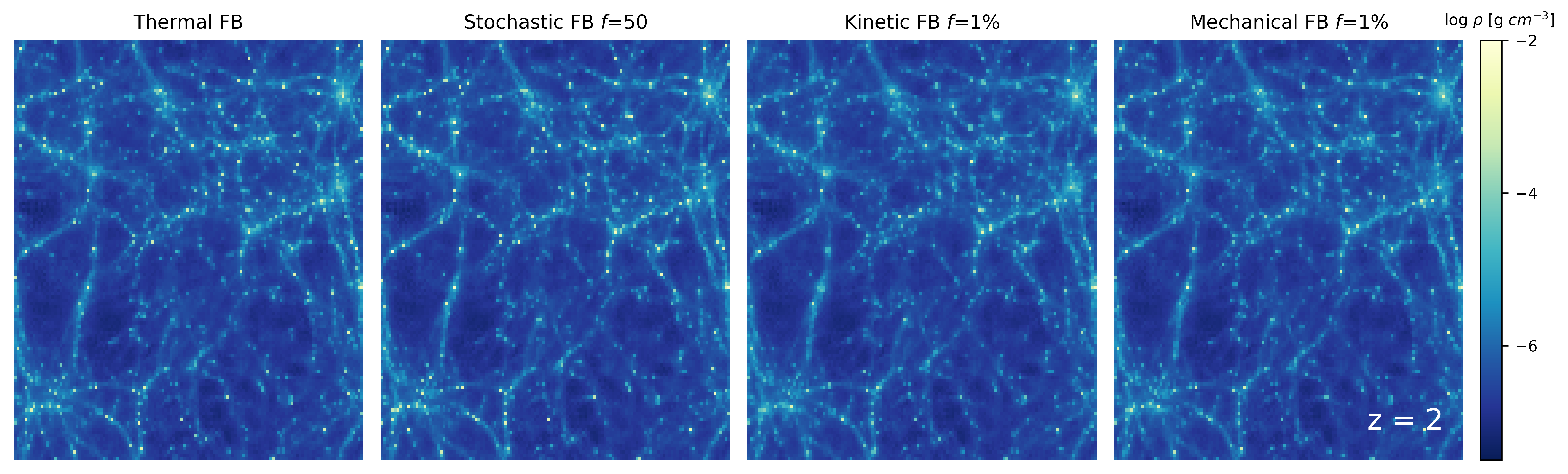
Figure 1: Density evolution of our cosmological simulations in 10 $h^{-1}$ Mpc³ box for our four feedback (FB) models: thermal, kinetic, stochastic, and mechanical in the 1st, 2nd, 3rd, and 4th columns, respectively, with the fiducial parameters in section 2.4. We show projected gas density at $z=0,z=1$, and $z=2$ in the top, middle and bottom rows, respectively.

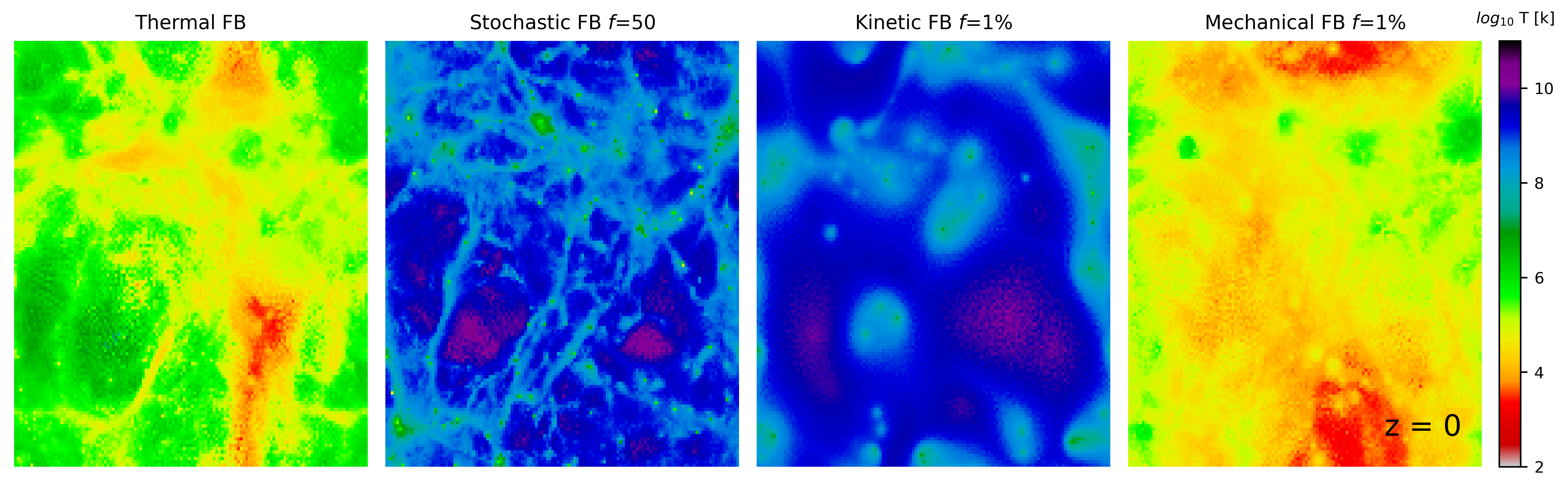
Figure 2: The same as Figure 1 but for temperature maps of our cosmological simulations for the four feedback models at $z=0$.

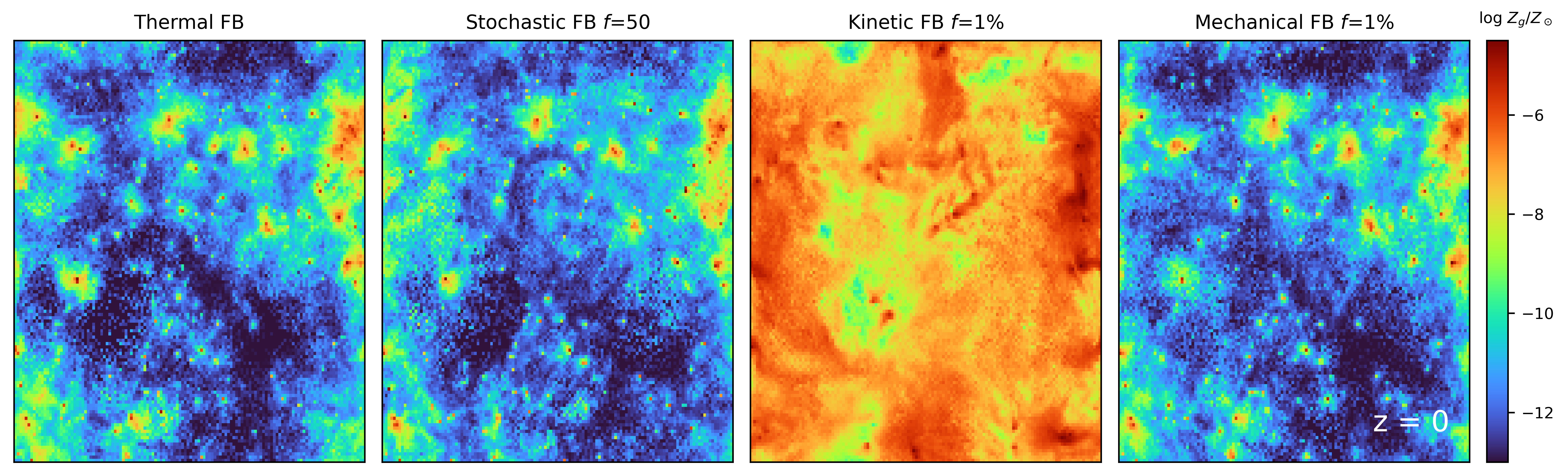
Figure 3: The same as Figure 1 but for the gas-phase metallicity, $\log Z_{\rm g}/Z_{\odot}$, in our cosmological simulations for the four feedback models at $z=0$.

3.2 Gas-phase diagram

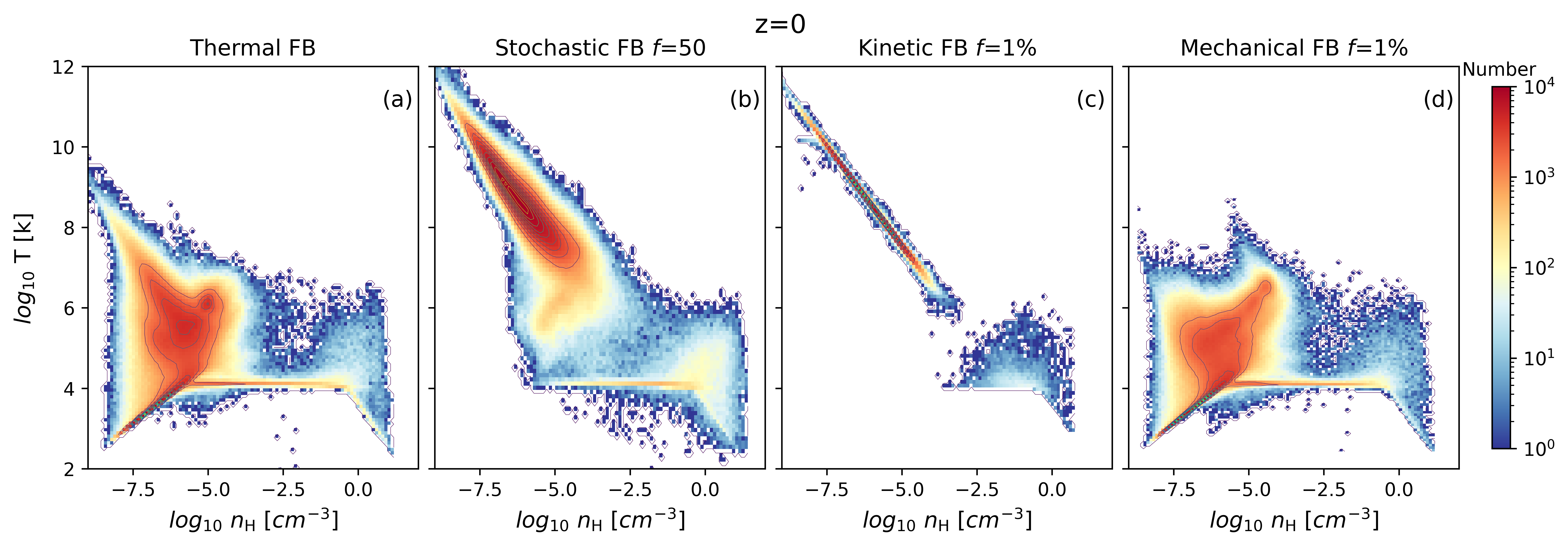
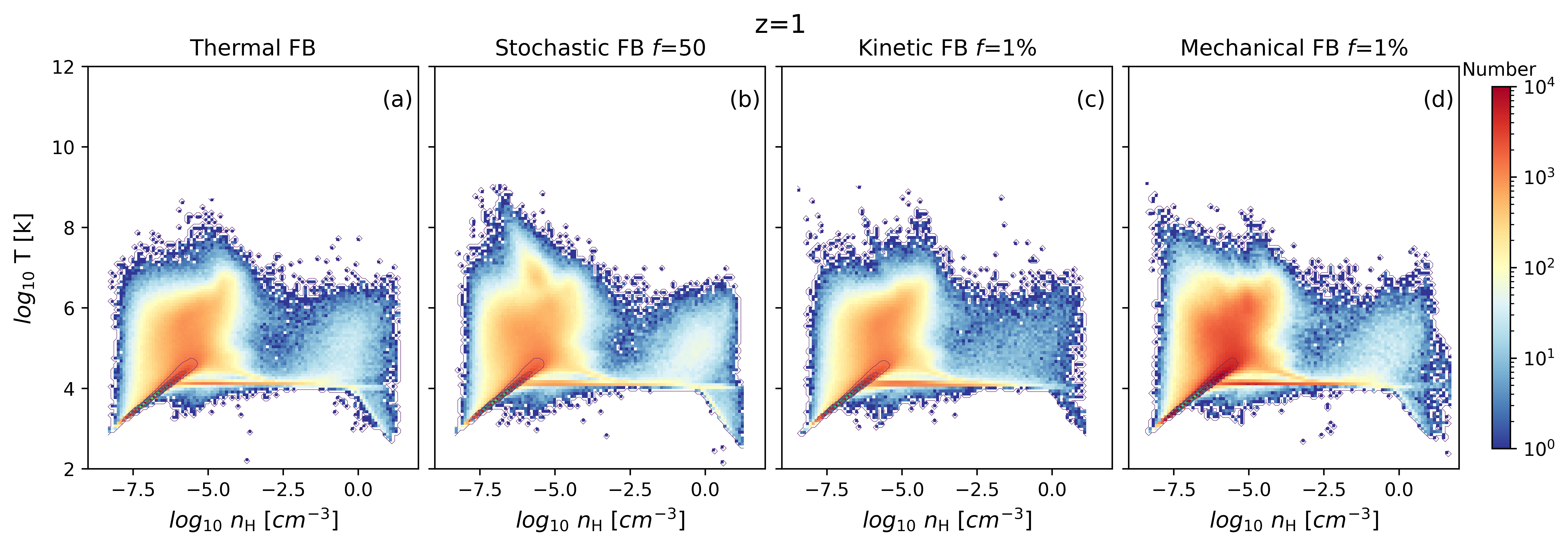
Figure 4: Density-temperature phase space diagrams for thermal (panel a), kinetic (panel b), stochastic (panel c), and mechanical (panel d) feedback models. Each panel shows the temperature as a function of hydrogen number density with the colour contour indicating the number density of the gas particles in the entire simulation volume at $z=0$.

Figure 5: The same as Figure 5 for $z=1$.

As described in Davé et al. (2001), the baryons in the universe are found in four different regions of the gas phase diagram: (1) The diffuse region (low temperature $T<10^{5}$K and low density $\rho$) contains adiabatic gas outside galaxies with no specific role. (2) The condensed region (low temperature $T<10^{5}$K and high density $\rho$) contains stars and cool gas inside galaxies. (3) The hot region ($T>10^{7}$K) contains the hot gas in galaxy clusters. (4) The warm-hot region ($10^{5}K<T<10^{7}$K) contains the baryons in the IGM. Such matter surrounding galaxies more closely can be observed with metal absorption lines and called CGM (Péroux & Howk, 2020).

Figure 5 shows the density-temperature phase space diagram at $z=0$ for the four feedback models with our fiducial parameters. The main noticeable feature is the different behaviours of the warm hot region. The diagrams of the thermal and mechanical models show two bumps at two different temperatures: the first bump is at $T\sim 10^{4}$K which corresponds to the peak of hydrogen cooling temperature, and the second bump is at $T\sim 10^{5}$K which corresponds to the peak of helium cooling.

The straight horizontal line at temperature $T\sim 10^{4}$K is caused by the cooling function sharply dropping below $T\sim 10^{4}$K (see Fig.13 of Kobayashi & Taylor 2023), which prevents gas cooling until it reaches very high density. Note that molecular cooling is not included, which would weaken this behaviour. At high densities, there are more star-forming particles in the stochastic feedback model than in the other models.

The gas phase temperature-density diagram for the kinetic feedback has a strange behaviour as most of the gas is hot and diffuse; this is due to the cooling function used in our simulations, which drops down when the particles are heated beyond $\sim 3\times 10^{5}$ K. This figure supports the prediction that the stochastic feedback will end up with the same behaviour as the kinetic one. These diagrams indicate that the mechanical feedback is a better model for this resolution.

The drastic changes for the kinetic and stochastic feedback happen after $z=1$ (see section 3.4), and Fig. 5 shows the gas phase diagram of the four models at $z=1$ where there is no significant difference between the models. If we look closer, the mechanical feedback has a slightly larger amount of warm gas (at T$\sim 10^{5}$ K); this is due to its efficiency, making the non-star forming gas particles either heated or ejected.

3.3 Cosmic Star Formation Rate

Figure 6 shows the cosmic SFR history obtained with each of the four feedback models with fiducial parameters. The SFR increases with time until the cosmic noon at redshift $\sim 2$, where the SFR was at its maximum. It decreases from $z\sim$ 2 to the present day because most of the cold gas has already turned into stars, but also because the formation of stars is suppressed by the presence of more supernova and AGN feedback. These test runs with a limited box size do not have very massive galaxies and galaxy clusters, which may explain our SFRs are lower at $z<\kern-11.99998pt\lower 4.73611pt\hbox{$\sim$}~{}2$ than observed. The stochastic feedback shows a similar behaviour with a slightly higher SFR (due to weaker feedback). In the kinetic case, the feedback impact can only be seen after sufficient star formation has occurred (i.e. at $z<\kern-11.99998pt\lower 4.73611pt\hbox{$\sim$}~{}$ 6). After $z=6$, the feedback is too strong, and star formation is suppressed too much, compared with the observations. We retrieve the same behaviour for the mechanical feedback with a less strong suppression of SFRs. Observational data are taken from Madau & Dickinson (2014) (grey cross) and Driver et al. (2018) (pink plus).

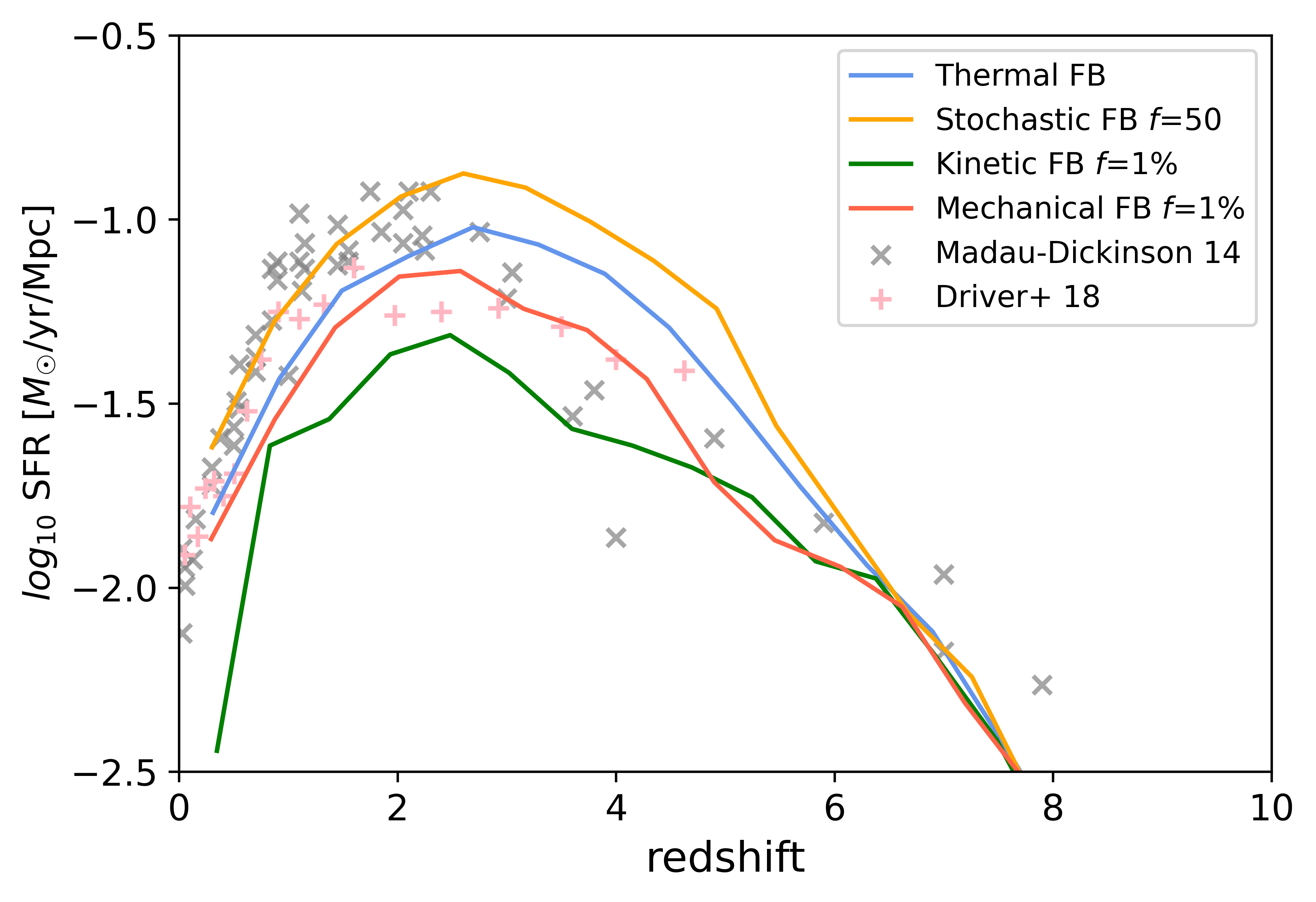
Figure 6: Cosmic star formation rate history of our 10 $h^{-1}$ Mpc simulations with our different feedback models: thermal (blue), stochastic (orange), kinetic (green), and mechanical (red). The observational data are taken from Madau & Dickinson (2014) (grey cross) and Driver et al. (2018) (pink plus).

3.4 Redshift evolution

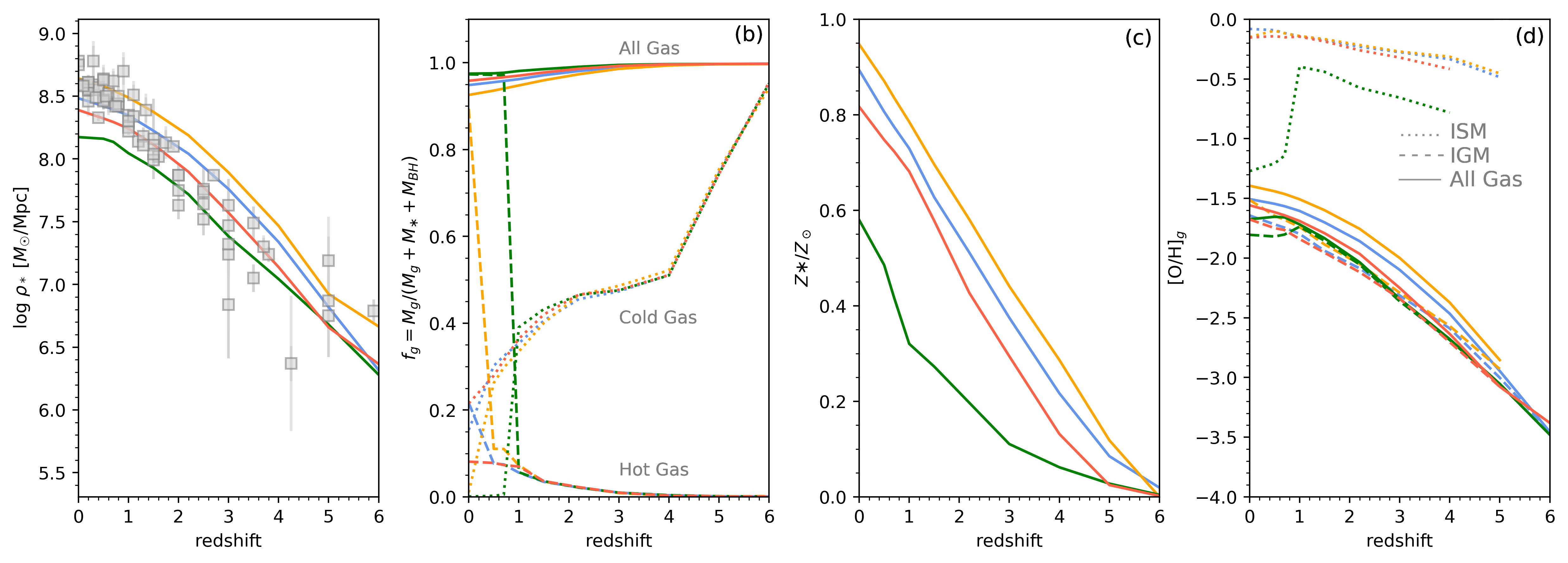
Figure 7: (a) Stellar mass density as a function of redshift, comparing to the observational data (grey square) taken from Madau & Dickinson (2014). (b) Cosmic gas fraction $f_{\rm g}\equiv M_{\rm g}/(M_{\rm g}+M_{*}+M_{\rm BH})$ for all gas (solid lines), hot gas ($T>10^{6}$K, dashed lines), and cold gas ($T<1.5\times 10^{4}$K, dotted lines). (c) Cosmic stellar metallicity evolution. (d) Gas-phase oxygen abundances evolution for all gas (solid lines), ISM (dotted lines), and IGM (dashed lines). In all panels, the thermal, stochastic, kinetic, and mechanical feedbacks are always shown in blue, orange, green, and red, respectively.

In Figure 7, we investigate the redshift evolution of different cosmic quantities of the gas and stars in our simulations. The panel 7a shows the stellar mass density as a function of redshift, obtained with our four feedback models. The kinetic model has the lowest stellar density at all redshifts plotted here since, as shown in the cosmic SFR, it is the strongest feedback that suppresses star formation the most. Our simulations follow a similar trend as observational data from Madau & Dickinson (2014). However, at $z>1$, the kinetic and mechanical feedback seems to fit better, while at $z<1$, the thermal and stochastic feedback work better.

The panel 7b shows the gas fraction defined as $f_{\rm g}$ $\equiv$ $M_{\rm g}/(M_{\rm g}+M_{*}+M_{\rm BH}$) as a function of redshift for the four feedback models. At $z>4$, the total gas fraction (solid lines) is $f_{\rm g}\sim 100\%$ for all models. From $z=4$, the total gas fraction decreases to $f_{\rm g}=94\%$, $92\%$, $97\%$, and $96\%$ at $z=0$, respectively for thermal, stochastic, kinetic, and mechanical feedback. All these are comparable with the observational estimates (e.g., $f_{\rm g}$ = 0.91-0.95 in Madau & Dickinson 2014). The stochastic feedback gives the smallest total gas fraction, and despite the large amount of hot gas in Figure 5, more gas is turned into stars overall (as shown in Fig. 7a). The kinetic feedback has the largest total gas fraction.

The dashed and dotted lines show the hot and cold gas fractions with $T>10^{6}$ and $T<1.5\times 10^{4}$ K, respectively. At $z>6$, most of the gas was cold in all models. The cold gas fraction decreases with time while the hot gas fraction increases, mainly due to stellar and AGN feedback. At $z\leq$2, the cold gas fraction differs depending on the feedback models. The kinetic model has the highest cold gas fraction, which may be explained by the lower SFR than the other models. The gas is drastically heated in the kinetic model at exactly $z=1$ due to the high efficiency of stellar feedback, this transition is not caused by our redshift binning but is real due to the nature of this feedback model. Around this redshift, a large number of gas particles are heated above $10^{5}$ K, where the cooling rate is low (as explained in section 3.2), and are ejected from galaxies, suddenly increasing the hot gas fraction. A similar behaviour is observed for the stochastic feedback later on at $z=0.5$, however, it is less sharp and evolves up to $z=0$. This extreme temperature change starts exactly at $z<1$ and $z<0.5$ for the kinetic and stochastic feedback, respectively. And the difference between $z=0$ and $z=1$ is clearly observed in the gas-phase density-temperature diagrams in Fig. 5 and Fig. 5.

The panel 7c shows the stellar metallicity across cosmic time for the four models, which increases as time followed by star formation. The kinetic model has the lowest stellar metallicity at all redshifts since fewer stars are produced than in any other models. It is clear that the supernova feedback model has an impact on the present-day stellar metallicity, with $Z_{*}/Z_{\odot}$= 0.89, 0.94, 0.57, 0.81 at $z=0$ for thermal, stochastic, kinetic, and mechanical feedback, respectively.

The panel 7d shows the evolution of oxygen abundance with time with the four feedback models for all the gas (solid lines), the ISM (dotted lines) and the IGM (dashed lines), separately. As defined in Kobayashi et al. (2007) and Taylor & Kobayashi (2016), the ISM is all gas particles in galaxies identified by the Friend of Friend algorithm (Springel et al., 2001b), and the IGM is all the other gas particles. The kinetic feedback has a lower oxygen abundance because it has less star formation, therefor fewer heavy elements are produced by supernovae. From $z=1$, the oxygen abundance is reduced in the ISM due to the winds that eject the oxygen-enhanced gas outside the galaxy, but also due to dilution, where all matter is mixed up and fills the ISM with hydrogen, which explains the drop in the plot. Table 1 summarizes the values of the cosmic stellar mass density $\log\rho_{\ast}$, gas fraction $f_{\rm g}$ (for all gas, hot gas, and cold gas), stellar metallicity $Z_{\ast}/Z_{\odot}$, and gas-phase oxygen abundance $[\mathrm{O/H}]_{\rm g}$ (for all gas, ISM, and IGM) at $z=0$, for the four feedback models.

FB Model	Thermal	Stochastic	Kinetic	Mechanical
$\log\rho_{\ast}$	8.483	8.642	8.173	8.389
$f_{\mathrm{g}}$ (All Gas)	0.948	0.925	0.974	0.958
$f_{\mathrm{g}}$ (Cold Gas)	0.154	0.0103	0.0007	0.215
$f_{\mathrm{g}}$ (Hot Gas)	0.216	0.893	0.973	0.081
$Z_{\ast}/Z_{\odot}$	0.893	0.947	0.974	0.816
$[\mathrm{O/H}]_{\mathrm{g}}$ (ISM)	-0.080	-0.148	-1.272	-0.152
$[\mathrm{O/H}]_{\mathrm{g}}$ (IGM)	-1.643	-1.512	-1.805	-1.676
$[\mathrm{O/H}]_{\mathrm{g}}$ (All Gas)	-1.506	-1.393	-1.674	-1.557

Table 1: Cosmic stellar mass density $\log\rho_{\ast}$, gas fraction $f_{\rm g}$ (for all gas, hot gas, and cold gas), stellar metallicity $Z_{\ast}/Z_{\odot}$, and gas-phase oxygen abundances $[\mathrm{O/H}]_{\rm g}$ (for all gas, ISM, and IGM) of the thermal, stochastic ($f=50$), kinetic ($f=1\%$) and mechanical ($f=1\%$) feedback models at $z=0$.

3.5 Mass–Metallicity Relations

3.5.1 Stellar Populations

Figure 8 shows the stellar mass–metallicity relations (MZRs) for the four feedback models, with the integrated metallicity of stars in galaxies weighted by the V-band luminosity of star particles. In our simulations, a star particle is not a single star but a set of many. We consider a star particle a simple stellar population (SSP, i.e. stars with the same age and metallicity but different masses). V-band luminosities of star particles are calculated using the Binary Population and Spectral Synthesis (BPASS) code version 2.2.1 (Stanway & Eldridge, 2018). The stellar metallicity of galaxies is measured in a 15 kpc projection from the galactic centre. The lines in Figure 8 represent the median of the simulated galaxies, while the shaded areas display the $1\sigma$ scatter. The solar metallicity used in the figure is $Z_{\odot}=0.015$.

Our thermal and stochastic models tend to overproduce metals compared with the local observations (black dashed line, with the grey shade for 1$\sigma$) taken from Zahid et al. (2017). Our kinetic feedback is not producing enough metals due to the lower SFR and not keeping enough metals in stars because of the kick velocity that drives the metals out of the galaxy. Among our four models, mechanical feedback gives the closest matches to the observed relation from Zahid et al. (2017) at $z=0$, with this resolution. We aim to confirm this by running even higher resolution in a larger volume of cosmological simulations in our future work.

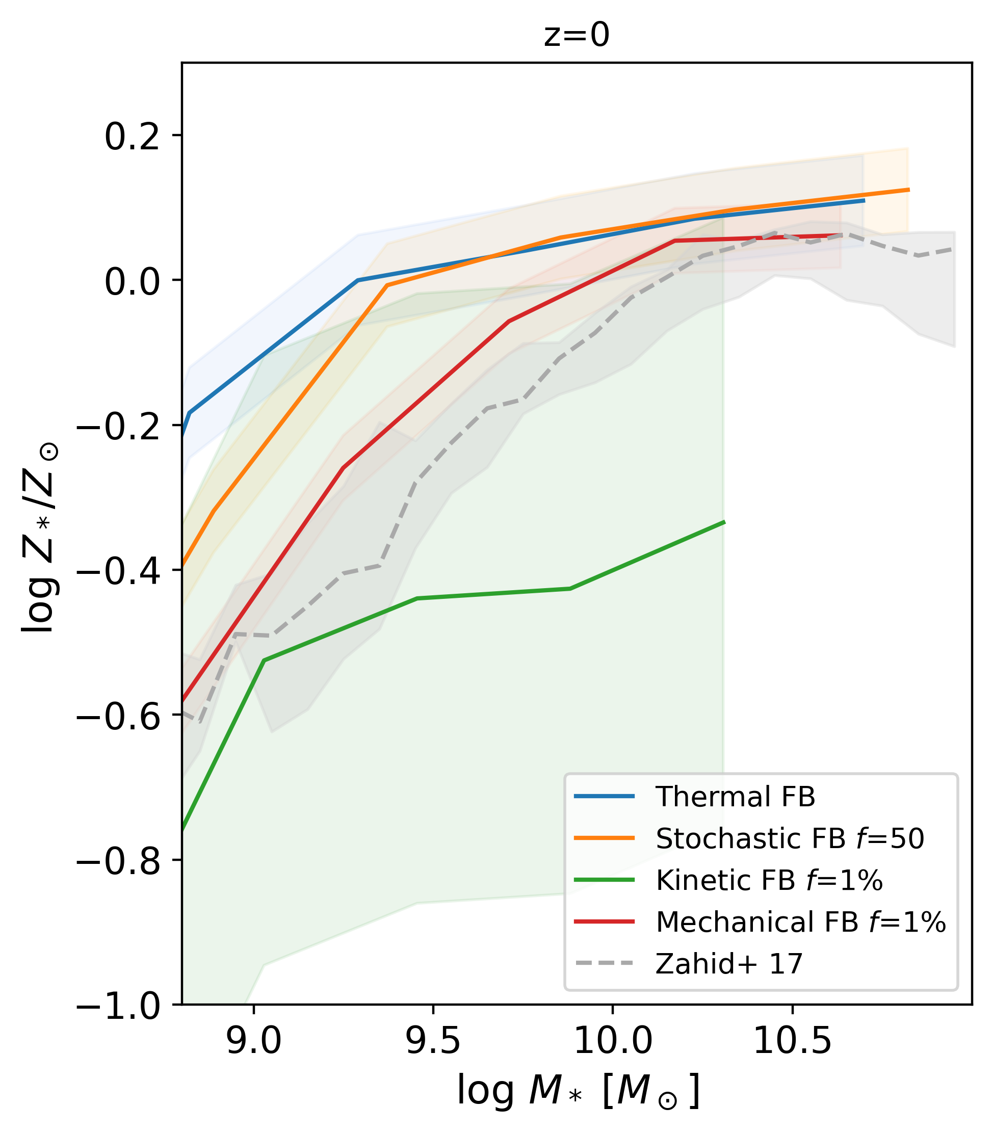
Figure 8: Stellar mass–metallicity relations with thermal (blue), stochastic (orange), kinetic (green), and mechanical (red) feedback models. The stellar metallicity is V-band luminosity-weighted. The lines are for medians and the shaded areas show the 1$\sigma$ scatter. The observational data are taken from Zahid et al. (2017) (grey dashed line, with 1$\sigma$ scatter).

3.5.2 Gas phase

Figure 9 shows the gas-phase MZRs with our four feedback models. We calculate the gas-phase “metallicity” of galaxies by measuring the gas oxygen abundance within 15 kpc from each galactic centre, weighted by the SFRs of gas particles to compare with observations, which are weighted by emission lines. Not many gas particles are forming stars with the current simulation volume and resolution, particularly at the massive end. Therefore, we have limited data points for SFR-weighted gas-phase metallicities. Consequently, we show the metallicities of galaxies (points), in addition to a fit (linear fit of medians; solid lines) in Fig. 9. The solar oxygen abundance adopted for our nucleosynthesis yields is $\sim$ 8.76. At $z=0$, the kinetic feedback gives the highest gas-phase metallicity ($\sim$ 9.1 dex), which is possibly due to the strong ejection of metal-poor gas. From this figure (namely scatter plot), we can conclude that for relatively low-mass galaxies at $\sim 10^{9}M_{\odot}$, the thermal and mechanical feedbacks are in reasonably good agreement with the observed gas-phase MZR from Kewley & Ellison (2008) (grey dashed line). The stochastic feedback seems to give a shallower slope than observed. With the mechanical feedback, higher-mass galaxies ($\sim 10^{10}M_{\odot}$) tend to have slightly lower metallicities than in Kewley & Ellison (2008), and are more comparable with Curti et al. (2020)’s observation (brown dashed line).

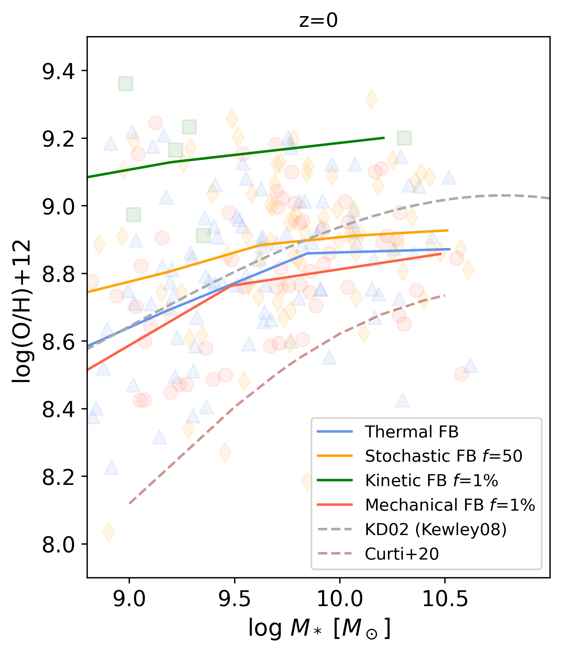
Figure 9: Gas-phase mass–metallicity relations with thermal (blue; triangles), stochastic (orange; diamonds), kinetic (green; squares), and mechanical (red; circles) feedback models. The SFR-weighted, gas-phase oxygen abundances of galaxies (number ratios relative to hydrogen) are shown. The observational data (grey dashed line) are from Tremonti et al. (2004) with the ‘KD02’ scale in Kewley & Ellison (2008), and from Curti et al. (2020) (brown dashed line).

It is important to note that while the shape of the stellar and gas-phase MZR is relatively robust against the methods used for the metallicity determination, the absolute amplitude of the stellar and gas-phase metallicity measurement of galaxies are still quite uncertain (e.g., Goddard et al. 2017 for stellar metallicity measurements with different stellar population synthesis codes and stellar templates and Maiolino & Mannucci 2019 for a review of the various methods for the gas-phase metallicity determination). This can also be seen in Fig. 10 and 11, where multiple sources of the metallicity measurements are included. It is very important to obtain the absolute values of metallicities of both stellar and gas-phase in observations.

3.5.3 Stellar MZR evolution

Figure 10 shows the stellar MZRs from $z=0$ to 3 for the four feedback models. At higher redshifts, all models systematically give lower metallicities at a given mass, showing very similar differences among the models ($\sim$ 0.2 dex from $z=3$ to 0). At all shown redshifts, the thermal feedback always produces slightly more metals than the other models. The low cosmic SFR with the kinetic feedback results in significantly lower stellar metallicities than in the other models. At the low-mass end, the stochastic feedback gives metallicities slightly lower than the thermal feedback by $\sim$ 0.1 dex. Overall, the supernova feedback has a more significant impact on the metallicity at the low-mass end where low-mass galaxies eject more metals (Kobayashi et al., 2007).

The mechanical feedback seems to give the best match to the observations at $z=0$, although the observed stellar metallicities at higher redshifts are either lower or of galaxies with limited overlap in mass compared to the model prediction. In the observations, massive galaxies have super-solar metallicities at $z=0$, which disappear at $z=3$. At $z=0$, as already shown in Fig.8, our model agrees well with the latest analysis by Zahid et al. (2017), although these give significantly higher metallicities than in Gallazzi et al. (2005). At $z=0.7$, although there is no overlap in the mass range, data from Gallazzi et al. (2014) is more consistent with our kinetic model. However, this data set does not reject the other models if we consider the significant offset between Zahid et al. (2017) and Gallazzi et al. (2005) data at $z=0$. We also note the large error bars of $\sim 0.2$ dex for these data. Our mechanical model seems consistent with the Hubble Space Telescope observations at $z=$ 1.1–1.6 (Estrada-Carpenter et al., 2019). These data suggest that the mass–metallicity relation has not significantly evolved since $z\sim 0$ at least at the massive end, contrary to Gallazzi et al. (2014) at $z\sim 0.7$. At $z=3$, the UV observations from Cullen et al. 2019 are for Fe abundances, are shifted by $+0.5$ dex taking account of [O/Fe], but still about $0.2$ dex lower than our predicted metallicities.

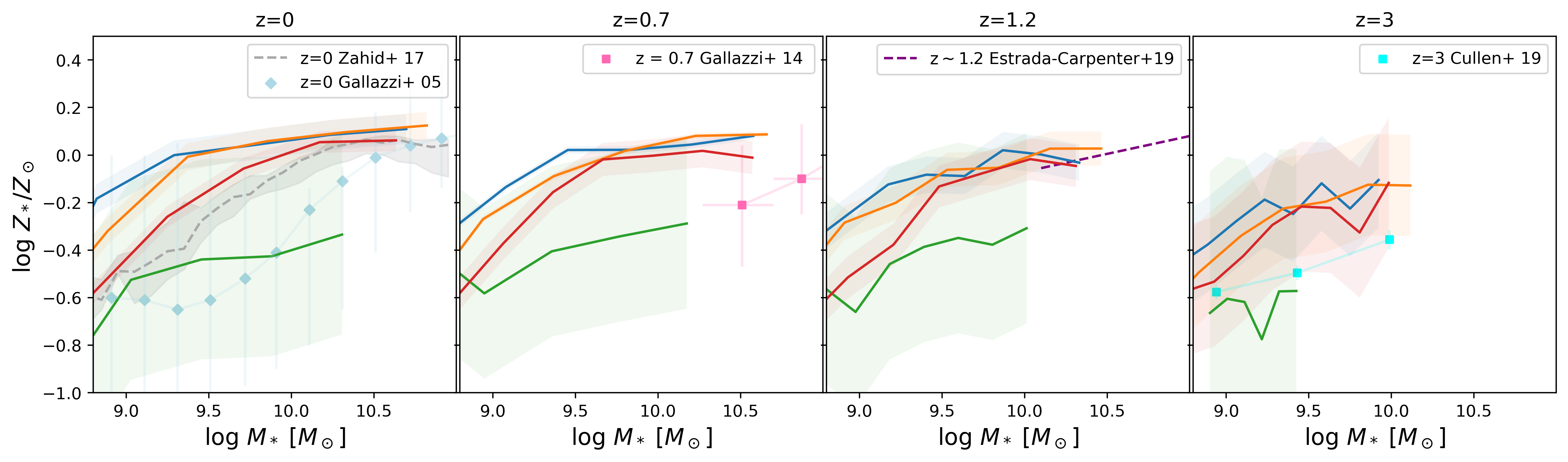
Figure 10: Evolution of the luminosity-weighted stellar MZRs with thermal (blue), stochastic (orange), kinetic (green), and mechanical (red) feedback models. The solid lines are for the medians, and the shaded areas show the $1\sigma$ scatter. Observational data are taken from Zahid et al. (2017, $z=0$), Gallazzi et al. (2005, $z=0$), Gallazzi et al. (2014, $z=1.2$), and Cullen et al. (2019, $z=3$, with $+0.5$ dex shift for [O/Fe]).

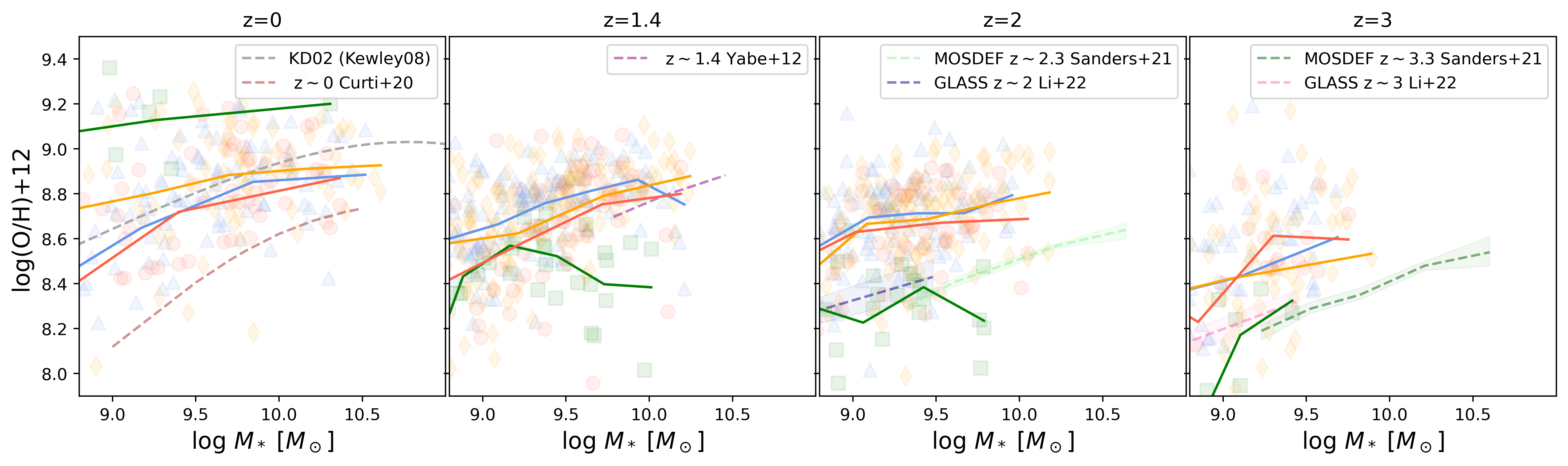
Figure 11: Evolution of the SFR-weighted gas-phase MZRs with thermal (blue; triangles), stochastic (orange; diamonds), kinetic (green;squares), and mechanical (red; circles) feedback models. The solid lines indicate the linear fit to the individual galaxies shown by the symbols with the same colour. Observational data are from Tremonti et al. 2004 ($z=0$) with the KD02 scale in Kewley & Ellison (2008, $z=0$), Curti et al. (2020, $z=0$), Yabe et al. (2012, $z=1.4$), Sanders et al. (2021, $z\sim$ 2–3), Li et al. (2022, $z\sim$ 2–3).

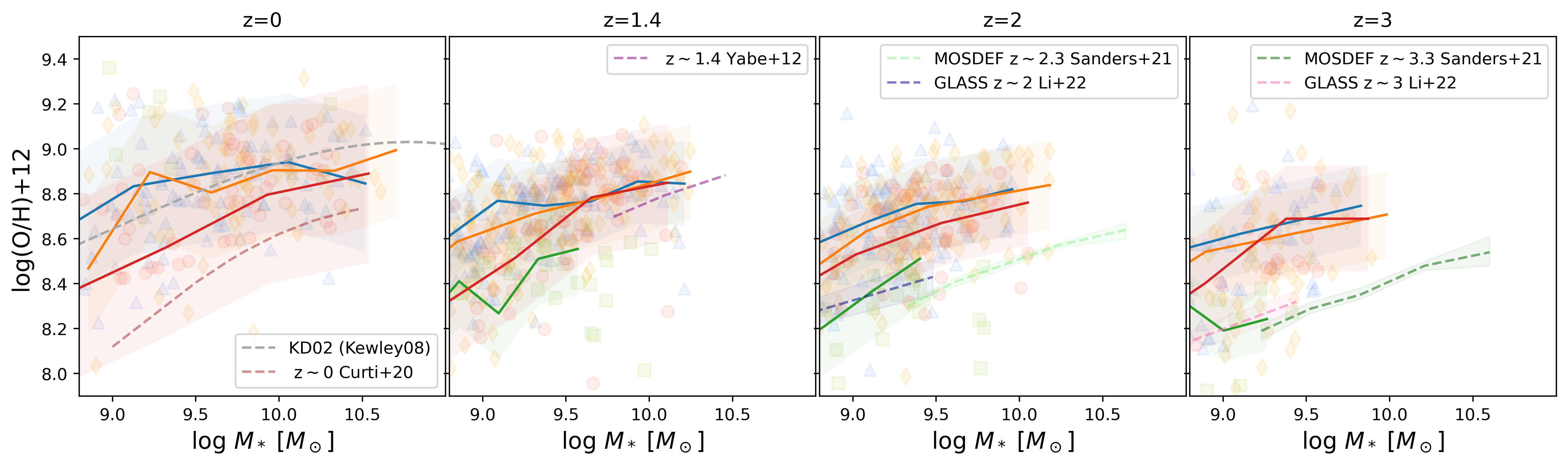
Figure 12: Evolution of the young stellar MZRs (solid lines) comparing to the gas-phase metallicities (symbols, the same as in Fig. 11). The solid lines are the medians of the luminosity-weighted stellar MZRs for stars younger than $0.1$ Gyr, and the shaded areas show the $1\sigma$ scatter.

3.5.4 Gas phase MZR evolution

Figure 11 shows the gas-phase MZRs from $z=0$ to 3 for the four feedback models. Although there is a significant scatter, and the sample is limited with our current resolution, there is a MZR at all redshifts. There is also a redshift evolution from $z=$3 to 0, where the metallicities decrease at higher redshifts notably for the kinetic feedback ($\sim$ 1.4 dex). The thermal feedback has only a mild evolution ($\sim$ 0.05 dex), and the stochastic and mechanical feedbacks have a significant evolution ($\sim$ 0.2 dex). At high redshifts, most low-mass galaxies have fast star formation enriching their ISM. However, the kinetic feedback suppresses this star formation, which leads to only a few metal-poor low-mass galaxies. As discussed previously, the drastic change in the kinetic feedback model, which occurs exactly after $z=1$ removing metal-poor gas and causing the metal-rich ($\sim$ 9.1 dex) galaxies (green squares) at $z=0$.

To verify the consistency between the stellar and gas-phase metallicities, we also show the metallicities of young stars since these are expected to be consistent with the metallicities of gas from which the stars were born. In Figure 12, we show the MZRs of young stars ($<$0.1 Gyr), comparing to the simulated gas-phase metallicities (symbols) and the observed gas-phase MZRs (dashed lines) at each redshift. The young stellar MZRs (solid lines) agree well with the simulated gas-phase metallicities. At $z=0$, the mechanical feedback increases with mass, similar to the observed MZRs. At higher redshifts, the kinetic feedback fits better, as in Figure 11. Note that no line is plotted for the kinetic feedback at $z=0$ because not many young stars form with the kinetic feedback.

The dashed lines represent observational data at various redshifts, which may be suffered by the uncertainties of the analysis methods, as already discussed. All observational data have been converted for the Kroupa IMF. At $z=0$, our mechanical feedback model most agrees with observed data from Tremonti et al. (2004) with the KD02 scale in Kewley & Ellison (2008), which gives 0.5–0.6 dex higher metallicities than in Curti et al. (2020). At $z=1.4$, although we only have galaxies at the low-mass end, we compare with observational data from Yabe et al. (2012) (converted to the method from Kewley & Dopita 2002 with the procedure given by Kewley & Ellison 2008) for massive galaxies. Then we find that the metallicity trend is comparable to our models. At higher redshifts, the MOSDEF (Sanders et al., 2021) and GLASS survey with NIRISS slitless spectroscopy on the James Webb Space Telescope (JWST) (Li et al., 2022) showed $\sim 0.1$ and $\sim 0.07$ dex evolution from $z\sim 2$ to $z\sim 3$, respectively, which is larger than in all our models ($\sim 0.07$ dex), except for the kinetic. The kinetic feedback model fits well with the laters, but as discussed previously, this model is underproducing stars, so this matching does not necessarily support kinetic feedback of supernovae.

4 Conclusions

Implementing four different methods of supernova feedback into our self-consistent cosmological chemodynamical simulations, we confirm that the modelling of feedback has a great impact on the mass–metallicity relations (MZRs), and can be constrained by spectroscopic observations of galaxies. In order to minimise other uncertainties, we have used the latest nucleosynthesis yields that can reproduce the observed elemental abundances of stars in the Milky Way (Kobayashi et al., 2020b, a), and aim to reproduce the stellar and gas-phase metallicities simultaneously.

We compare four supernova feedback models: The classic thermal and kinetic models, where supernova energy is either ejected in pure thermal form or with a partial kinetic kick; The stochastic model, similar to Dalla Vecchia & Schaye (2012), which heats a random number of neighbour gas particles with a fixed energy increase; And the mechanical model from Hopkins et al. (2018), which considers the work done during the Sedov-Taylor phase of supernova expansion. After performing a parameter study (Appendix A), we choose the following fiducial parameters from the observed cosmic SFRs (section 2.4): $f=1\%$, $f=50$, and $f=1\%$ for kinetic, stochastic, and mechanical feedback models, respectively. Cosmic SFRs are significantly reduced with the kinetic feedback, which is too strong and is not producing enough stars, even with only a tiny fraction of supernova energy converted to a kick velocity. On the other hand, thermal and stochastic models are slightly overproducing stars at $z>\kern-11.99998pt\lower 4.73611pt\hbox{$\sim$}~{}2$. Mechanical feedback gives a better match to the observed cosmic SFRs (Fig. 6).

Despite fairly similar cosmic SFRs, we find a drastic change in the heating history of the ISM at $z\sim 1$ with the kinetic feedback, and at $z\sim 0.5$ with the stochastic feedback. This can be clearly seen in the gas-phase space diagram (Figs. 5 and 5) as the hot diffused gas, as well as in the spatial distribution of temperatures (Fig. 2). The spatial distribution of metals (Fig. 3) are fairly similar, except for the kinetic feedback.

Galaxy MZRs are greatly affected by the supernova feedback models. Strong supernova feedback makes star formation inefficient in the galaxy, which results in lower stellar metallicities of galaxies (Fig.8). However, this is not the case for gas-phase metallicities, particularly with kinetic feedback (Fig.9). We find that young ($<0.1$ Gyr) stellar metallicities are consistent with the gas-phase metallicities. Considering both stellar and gas-phase MZRs, our mechanical feedback seems the most plausible in order to explain the observational data of present-day galaxies.

Finally, we show the time evolution of the MZRs. As expected, both stellar and gas-phase metallicities become lower at higher redshifts in all feedback models. With our mechanical feedback, the predicted evolution of stellar MZR is in reasonably good agreement with the observations up to $z\sim 3$ (Fig.10). Our kinetic feedback model gives too low stellar metallicities at all redshifts. For the gas-phase MZR, we find too large evolution in the kinetic model from $z\sim 3$ to 0, and less prominent evolution for the other models (Fig.11). The available observations at $z>1$ seem rather consistent with the kinetic model, and we will investigate this further by comparing higher resolution and larger volume simulations to distant galaxies with the JWST as well as those of a large sample from ongoing and future spectroscopic galaxy surveys on ground-based telescopes.

Data Availability

The simulation data can be shared on request.

Appendix A Star formation rates

We have chosen the fiducial model parameters in order to match the observed cosmic SFR history. Fig. 13 shows the SFRs as a function of redshift for different values of the feedback parameter $f$ as obtained for thermal, kinetic, stochastic and mechanical feedback models, in panels (a),(b), (c), and (d), respectively. For this figure we use a resolution of $N_{\mathrm{gas}}$=$N_{\mathrm{DM}}$=$96^{3}$. All curves show a peak in the SFRs at $z\sim 3$. The box size in our simulation is limited due to the computation time. As a result, it does not include the formation of very massive galaxies and galaxy clusters at low redshifts. This explains the observed SFR peaks around $z\sim 2-3$, which are expected to be more consistent with observations for a larger simulation volume. For the kinetic and mechanical models, a larger $f$ results in a more efficient formation across cosmic time, but not for the stochastic model. The results of our parameter study can be summarised as follows.

• Figure 13(a) shows the SFR for the thermal feedback. The SFR increases from $z\sim 10$ to $z\sim 3$, it decreases from $z\sim 3$ to the present day because: (1) more gas has already turned into stars, (2) more supernova feedback suppressing star formation, and (3) more AGN feedback.

• Figure 13(b) shows the cosmic SFR with the kinetic feedback for different parameter values $f$. It shows that at high redshifts, the slope is the same for all parameters, as stars have not formed yet in these simulations. The feedback impact can only be seen after sufficient star formation has occurred, i.e. around redshift $z=6$. At redshift $z\leq 6$, star formation is suppressed too much for $f>30\%$. Then, the SFR slightly increases around $z=3$. This wave-shaped SFR history is explained independently of the feedback method by self-regulation: strong feedback suppresses star formation, resulting in less stellar feedback, which will, in return, increase star formation. (starting roughly at $z\sim 4$ depending on the parameters). For a small parameter $f<30\%$, the SFR increases from $z\sim 6$ to $z\sim 2$, where the feedback starts suppressing star formation. The kinetic model with $f=0.1\%$ gives similar results to the thermal feedback. In order to demonstrate the impact of the kinetic part, we choose to use $f=1\%$ as our fiducial parameter. Overall, the kinetic feedback in our simulation is too strong and suppresses star formation too much, as even with $f=1\%$, the SFR peak remains too low compared to the observations.

• Figure 13(c) shows the cosmic SFR applying the stochastic feedback with different parameter values $f$. The SFR is larger for a larger $f$. This may be explained using Equation 3 where the energy increase $\Delta e$ is proportional to $f$. Thus a large $f$ results in a large $\Delta e$, which yields the right-hand side of Equation 4 to be small. Therefore, for a large $f$, Equation 4 is rarely satisfied. Hence only a small number of particles receive the energy increase and are impacted by the feedback. When the condition is not satisfied, feedback does not impact the gas particles, which do not receive heating energy. The particles keep getting cool by following the cooling function until their temperature reaches $10^{4}$K. Once the particles are cool, the pressure is lost, the mater collapses toward the cooling particles where the density increases, and then the cooling rate becomes high (i.e. it accelerates the cooling). These features are shown in the star-forming region (low temperature, high density) of the gas-phase space diagram (Fig. 5).

• Finally, mechanical feedback SFR is shown in Figure 13(d), where we retrieve a similar behaviour as for the kinetic feedback, but slightly less efficient. We also find that this method is more affected by numerical resolutions than the other models, and have presented higher resolution results only in the previous sections.

For each method, we select the following fiducial parameters: $f=1\%$ (kinetic feedback), $f=50$ (stochastic feedback), and $f=1\%$ (mechanical feedback).

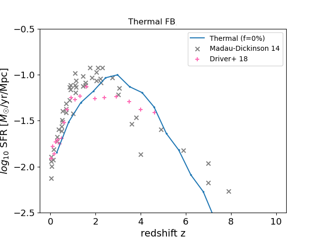
(a)

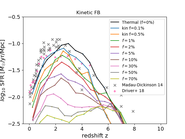
(b)

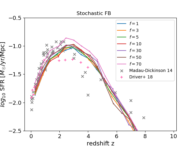
(c)

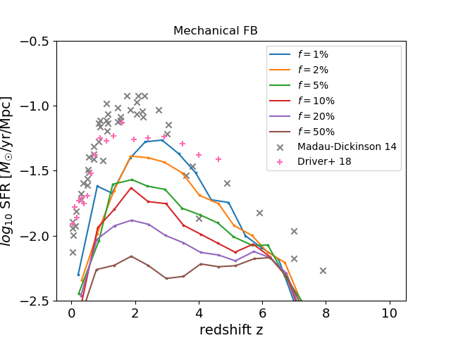
(d)

Figure 13: Cosmic SFRs for thermal, kinetic, stochastic and mechanical feedback models in panels (a), (b), (c) and (d) respectively. For each model we explore a wide range of feedback parameter $f$. The grey cross and magenta plus are observational data taken from Madau & Dickinson (2014) and Driver et al. (2018), respectively, from far UV to mid IR.

Appendix B Stellar Metallicities

In what follows, we compare the impact of the feedback parameter $f$ on the stellar MZR at $z=0$ for each model.

• The MZR for thermal feedback is shown in Figure 14(a), comparing the luminosity-weighted metallicity (blue) with the mass-weighted metallicity (orange). There is a $0.2$dex offset; the luminosity-weighted metallicity is higher because it is weighted for young and metal-rich stars.

• Figure 14(b) shows the MZRs using the kinetic feedback model with different parameter values $f$. It shows that overall the metallicity is always lower than the observed MZR. The metallicity is lower for stronger kinetic feedback (larger $f$) because a large kinetic velocity ejects more outflows, driving the metal-enriched gas out of the galaxy. As explained above, this difference is more visible in low-mass galaxies.

• Figure 14(c) shows the MZRs with the stochastic feedback. At the high-mass end, the MZR is not impacted by the parameter $f$ and the metallicities are always higher than observed. Lower mass galaxies ($M<10^{9}M_{\odot}$) have higher metallicities with a larger $f$. This agrees with what is discussed above for the SFR with the stochastic feedback where a larger $f$ produces more star formation, enhancing the metallicities.

• Finally, the mechanical feedback MZRs are shown in Figure 14(d) where we retrieve a similar behaviour as for the kinetic feedback. The metallicities are higher for a smaller $f$.

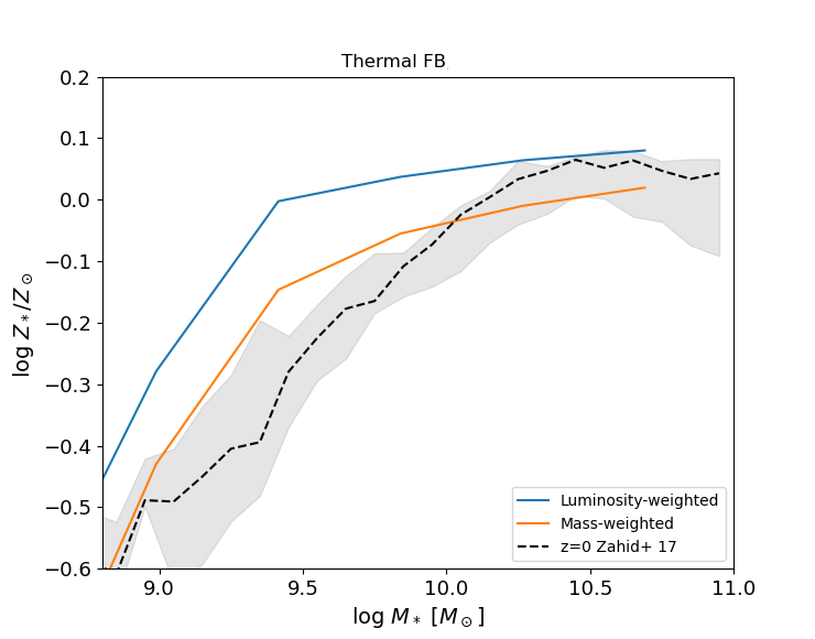
(a)

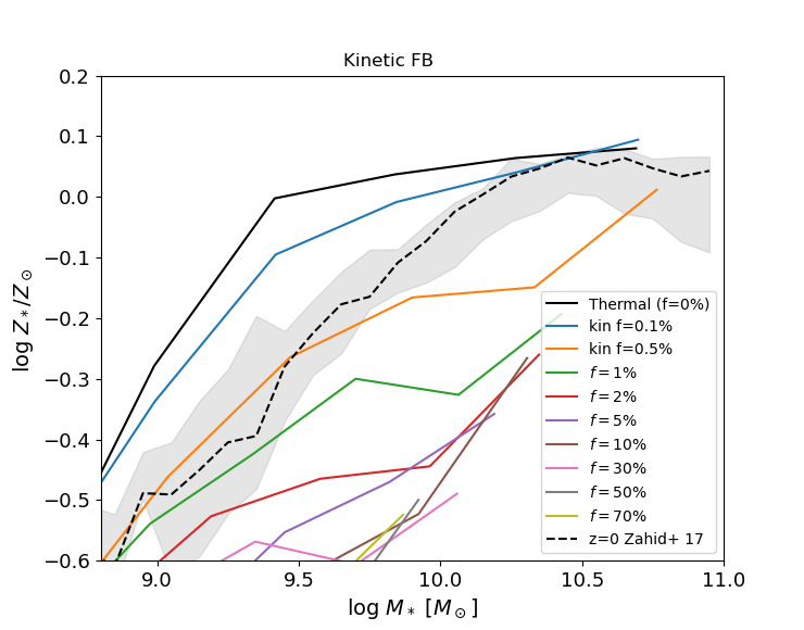
(b)

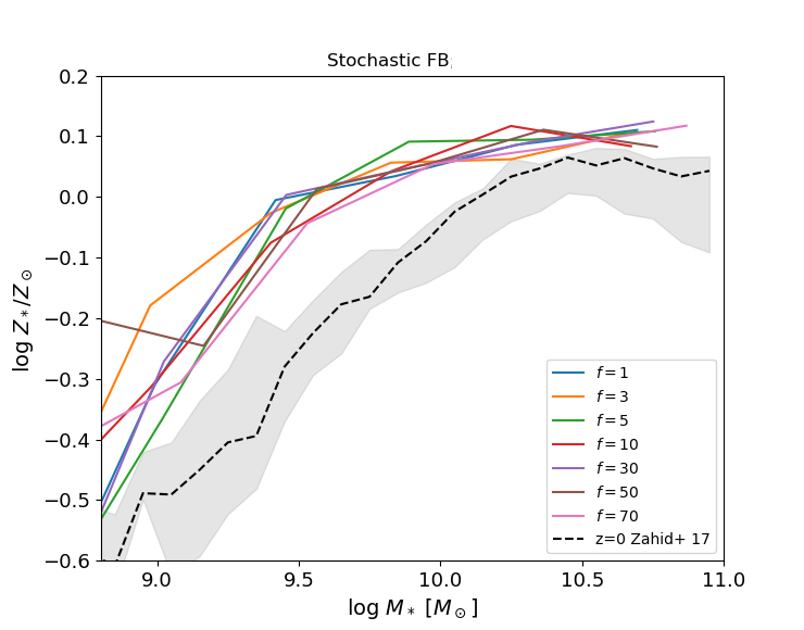
(c)

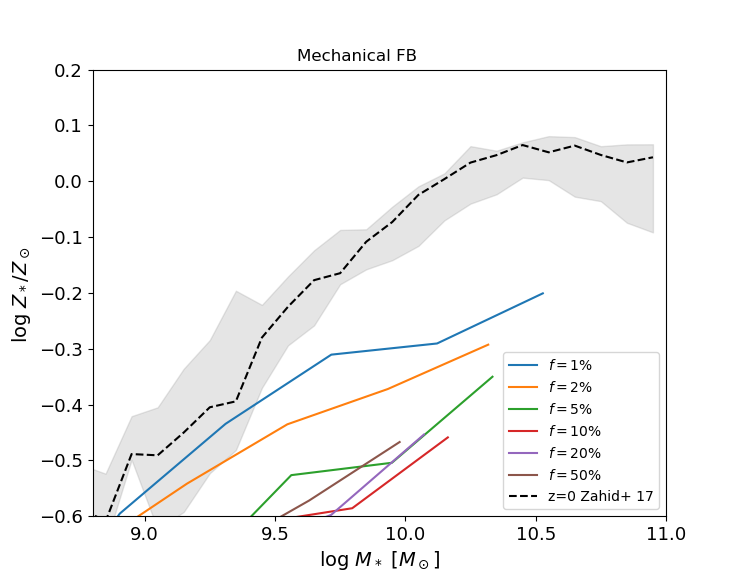
(d)

Figure 14: Stellar MZRs for thermal, kinetic, stochastic and mechanical feedback models are shown in panels (a), (b), (c) and (d), respectively. For the thermal feedback (panel (a)), we compare luminosity-weighted metallicity (blue) with mass-weighted metallicity (orange). For panels (b), (c) and (d), we explore a wide range of feedback parameters $f$, at $z=0$. The black dashed line and shaded are optical observational data taken from Zahid et al. (2017) of star-forming galaxies in the SDSS at $z=0$.

Appendix C Age dependence of the stellar MZRs

In Section 3.5.4, we have shown that young stellar MZRs are roughly consistent with gas-phase MZRs at $z=0$. Here, we show the MZR dependence on the age-unfolding at various redshifts, which might indicate when the stellar MZR is established.

Figure 15 compares the stellar MZRs with different stellar ages (ages of star particles) for the four feedback models. A clear time evolution is seen; younger stars tend to have higher metallicities. Stars $<0.1$ Gyr (blue line) look less metal-rich than green and orange lines at the massive end because of the small sample. The MZRs of stars younger than $\sim$1 Gyr are consistent with simulated gas-phase metallicities (grey points) at all redshifts. At $z\sim 3$, MZRs with 0.1–1 Gyr old stars (orange line) show a similar slope as the other MZRs plotted in this figure; these stars have formed around $z\sim 5$. At $z\sim 2$, MZRs with 1–2 Gyr old stars (green line) show significantly lower metallicities with a larger scatter; these stars have formed around $z\sim 5$. These might mean that MZRs are established at $z\sim 5$, which might be consistent with the lack of a clear MZR in the recent JWST observations of $z\sim 8$ galaxies (Curti et al., 2023). Better statistics would be required to investigate this further.

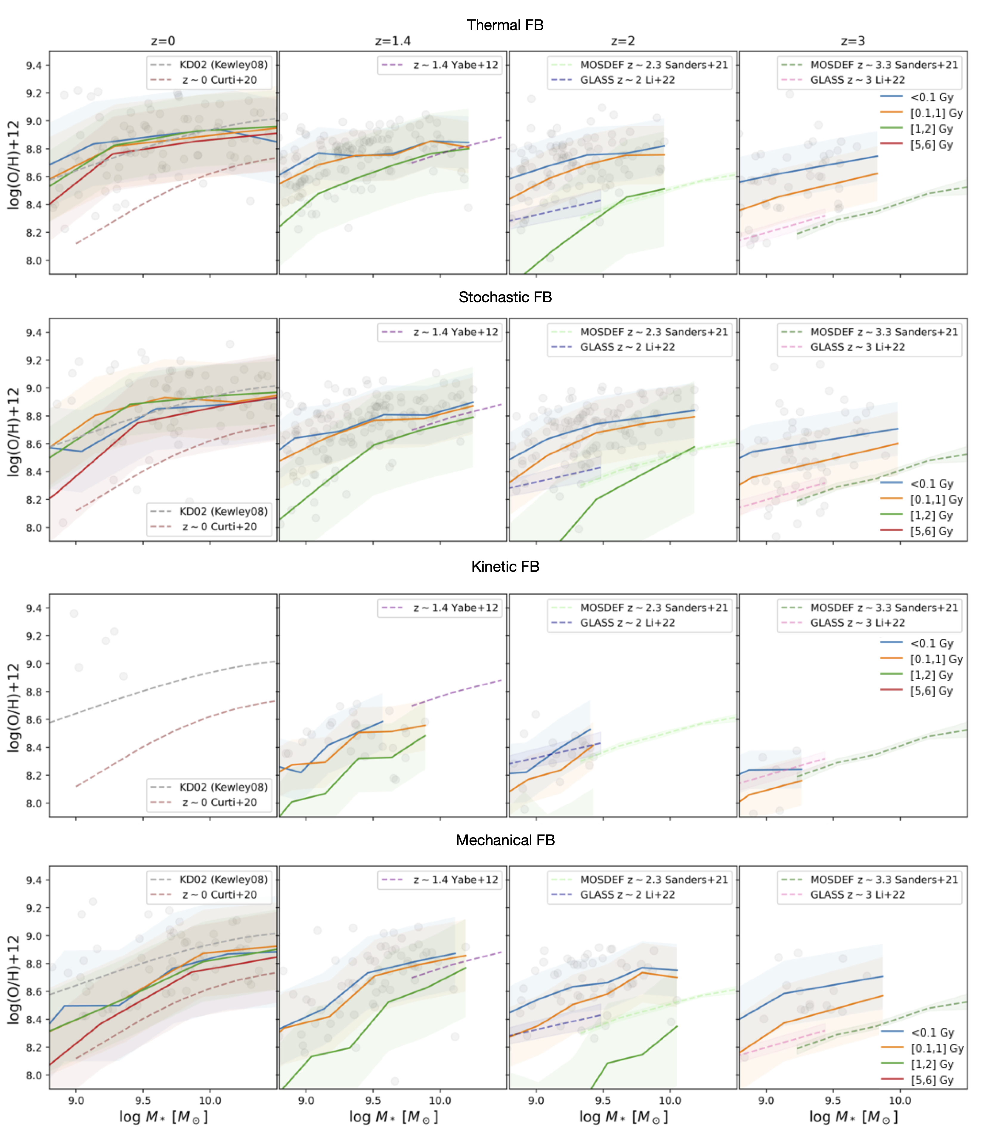
Figure 15: Evolution of luminosity-weighted stellar MZRs of galaxies with different ages of star particles: $<0.1$ (blue), 0.1–1 (orange), 1–2 (green), and 5–6 Gyr (red), comparing to the gas-phase metallicities of galaxies (grey points). From top panel to bottom, the figure shows thermal, stochastic, kinetic and mechanical feedback models. The solid lines are for medians, and the shaded areas show the $1\sigma$ scatter. The dashed lines represent the same observational data for the gas-phase MZRs as in Fig. 11.

References

- Belfiore et al. (2016) Belfiore F., Maiolino R., Bothwell M., 2016, MNRAS, 455, 1218
- Conroy (2013) Conroy C., 2013, ARA&A, 51, 393
- Cullen et al. (2019) Cullen F., et al., 2019, MNRAS, 487, 2038
- Curti et al. (2020) Curti M., Mannucci F., Cresci G., Maiolino R., 2020, MNRAS, 491, 944
- Curti et al. (2023) Curti M., et al., 2023, MNRAS, 518, 425
- Dalla Vecchia & Schaye (2012) Dalla Vecchia C., Schaye J., 2012, MNRAS, 426, 140
- Davé et al. (2001) Davé R., et al., 2001, ApJ, 552, 473
- Davé et al. (2019) Davé R., Anglés-Alcázar D., Narayanan D., Li Q., Rafieferantsoa M. H., Appleby S., 2019, MNRAS, 486, 2827
- Dekel & Silk (1986) Dekel A., Silk J., 1986, ApJ, 303, 39
- Driver et al. (2018) Driver S. P., et al., 2018, MNRAS, 475, 2891
- Dubois et al. (2016) Dubois Y., Peirani S., Pichon C., Devriendt J., Gavazzi R., Welker C., Volonteri M., 2016, Monthly Notices of the Royal Astronomical Society, 463, 3948
- Estrada-Carpenter et al. (2019) Estrada-Carpenter V., et al., 2019, ApJ, 870, 133
- Gallazzi et al. (2005) Gallazzi A., Charlot S., Brinchmann J., White S. D. M., Tremonti C. A., 2005, MNRAS, 362, 41
- Gallazzi et al. (2006) Gallazzi A., Charlot S., Brinchmann J., White S. D. M., 2006, MNRAS, 370, 1106
- Gallazzi et al. (2014) Gallazzi A., Bell E. F., Zibetti S., Brinchmann J., Kelson D. D., 2014, ApJ, 788, 72
- Gingold & Monaghan (1977) Gingold R. A., Monaghan J. J., 1977, MNRAS, 181, 375
- Goddard et al. (2017) Goddard D., et al., 2017, MNRAS, 466, 4731
- Hernquist & Katz (1989) Hernquist L., Katz N., 1989, ApJS, 70, 419
- Hopkins et al. (2014) Hopkins P. F., Kereš D., Oñorbe J., Faucher-Giguère C.-A., Quataert E., Murray N., Bullock J. S., 2014, MNRAS, 445, 581
- Hopkins et al. (2018) Hopkins P. F., et al., 2018, MNRAS, 477, 1578
- Katz (1992) Katz N., 1992, ApJ, 391, 502
- Kay et al. (2003) Kay S. T., Thomas P. A., Theuns T., 2003, MNRAS, 343, 608
- Kewley & Dopita (2002) Kewley L. J., Dopita M. A., 2002, ApJS, 142, 35
- Kewley & Ellison (2008) Kewley L. J., Ellison S. L., 2008, ApJ, 681, 1183
- Kimm et al. (2015) Kimm T., Cen R., Devriendt J., Dubois Y., Slyz A., 2015, MNRAS, 451, 2900
- Kobayashi (2004) Kobayashi C., 2004, MNRAS, 347, 740
- Kobayashi & Taylor (2023) Kobayashi C., Taylor P., 2023, arXiv e-prints, p. arXiv:2302.07255
- Kobayashi et al. (2007) Kobayashi C., Springel V., White S. D. M., 2007, Monthly Notices of the Royal Astronomical Society, 376, 1465
- Kobayashi et al. (2020a) Kobayashi C., Leung S.-C., Nomoto K., 2020a, ApJ, 895, 138
- Kobayashi et al. (2020b) Kobayashi C., Karakas A. I., Lugaro M., 2020b, ApJ, 900, 179
- Kroupa (2008) Kroupa P., 2008, in Aarseth S. J., Tout C. A., Mardling R. A., eds, , Vol. 760, The Cambridge N-Body Lectures. p. 181, doi:10.1007/978-1-4020-8431-7_8
- Larson (1974) Larson R. B., 1974, MNRAS, 169, 229
- Lequeux et al. (1979) Lequeux J., Peimbert M., Rayo J. F., Serrano A., Torres-Peimbert S., 1979, A&A, 80, 155
- Li et al. (2022) Li M., et al., 2022, The Mass-Metallicity Relation of Dwarf Galaxies at the Cosmic Noon in the JWST Era (arXiv:2211.01382)
- Lian et al. (2018) Lian J., Thomas D., Maraston C., Goddard D., Comparat J., Gonzalez-Perez V., Ventura P., 2018, MNRAS, 474, 1143
- Lin & Zu (2023) Lin Y., Zu Y., 2023, MNRAS, 521, 411
- Lucy (1977) Lucy L. B., 1977, AJ, 82, 1013
- Madau & Dickinson (2014) Madau P., Dickinson M., 2014, ARA&A, 52, 415
- Maiolino & Mannucci (2019) Maiolino R., Mannucci F., 2019, A&ARv, 27, 3
- McClure & van den Bergh (1968) McClure R. D., van den Bergh S., 1968, AJ, 73, 313
- Navarro & White (1993) Navarro J. F., White S. D. M., 1993, MNRAS, 265, 271
- Péroux & Howk (2020) Péroux C., Howk J. C., 2020, ARA&A, 58, 363
- Pillepich et al. (2018) Pillepich A., et al., 2018, MNRAS, 473, 4077
- Planck Collaboration (2020) Planck Collaboration 2020, Astronomy & Astrophysics, 641
- Press & Schechter (1974) Press W. H., Schechter P., 1974, ApJ, 187, 425
- Sanders et al. (2021) Sanders R. L., et al., 2021, ApJ, 914, 19
- Schaye et al. (2015) Schaye J., et al., 2015, MNRAS, 446, 521
- Sedov (1959) Sedov L. I., 1959, Similarity and Dimensional Methods in Mechanics
- Silk (2013) Silk J., 2013, ApJ, 772, 112
- Smith et al. (2018) Smith M. C., Sijacki D., Shen S., 2018, MNRAS, 478, 302
- Springel & Hernquist (2003) Springel V., Hernquist L., 2003, MNRAS, 339, 289
- Springel et al. (2001a) Springel V., Yoshida N., White S. D. M., 2001a, New Astron., 6, 79
- Springel et al. (2001b) Springel V., White S. D. M., Tormen G., Kauffmann G., 2001b, MNRAS, 328, 726
- Springel et al. (2005) Springel V., Di Matteo T., Hernquist L., 2005, MNRAS, 361, 776
- Stanway & Eldridge (2018) Stanway E. R., Eldridge J. J., 2018, MNRAS, 479, 75
- Sutherland & Dopita (1993) Sutherland R. S., Dopita M. A., 1993, ApJS, 88, 253
- Taylor (1950) Taylor G., 1950, Proceedings of the Royal Society of London Series A, 201, 159
- Taylor & Kobayashi (2014) Taylor P., Kobayashi C., 2014, MNRAS, 442, 2751
- Taylor & Kobayashi (2015) Taylor P., Kobayashi C., 2015, MNRAS, 448, 1835
- Taylor & Kobayashi (2016) Taylor P., Kobayashi C., 2016, MNRAS, 463, 2465
- Taylor et al. (2020) Taylor P., Kobayashi C., Kewley L. J., 2020, MNRAS, 496, 4433
- Tremonti et al. (2004) Tremonti C. A., et al., 2004, ApJ, 613, 898
- White & Frenk (1991) White S. D. M., Frenk C. S., 1991, ApJ, 379, 52
- White & Rees (1978) White S. D. M., Rees M. J., 1978, MNRAS, 183, 341
- Worthey et al. (1992) Worthey G., Faber S. M., Gonzalez J. J., 1992, ApJ, 398, 69
- Yabe et al. (2012) Yabe K., et al., 2012, PASJ, 64, 60
- Zahid et al. (2017) Zahid H. J., Kudritzki R.-P., Conroy C., Andrews B., Ho I. T., 2017, ApJ, 847, 18