One dimensional Bose-Einstein condensate under the effect of the extended uncertainty principle

Abstract

In this study, an analytical investigation was conducted to assess the effects of the extended uncertainty principle (EUP) on a Bose-Einstein condensate (BEC) described by the deformed one-dimensional Gross-Pitaevskii equation (GPE). Analytical solutions were derived for null potential, while, we used variational and numerical methods for harmonic oscillator potential. Subsequently, we analyzed the probability density, position, and momentum uncertainties as functions of the deformation parameter $\alpha$.

1 Introduction

The Gross-Pitaevskii equation (GPE) is fundamentally used to describe the behavior of a Bose-Einstein condensate (BEC) at very low temperatures ($T\rightarrow 0,\mathrm{K}$) 31 ; 32 . Originally, it appeared in the beginning as a model to study superfluids and the vortex lines modeled by a non-perfect Bose-Einstein gas GPE ; GPE1 ; GPE2 . The GPE is a nonlinear Schrödinger equation with cubic nonlinearity. It has been proven that the 1D cubic nonlinear Schrödinger equation satisfies a solitonic (shape-invariant) solution GPE4 , specifically, bright and dark soliton solutions for self-focusing and self-defocusing respectively. Several works have been done in the context of addressing the GPE experimentally, analytically, and numerically under various types of nonlinearity and potentials. To name a few, A. Weller et al. GPE5 experimentally investigated the oscillating and interacting matter wave dark solitons by releasing a BEC from a double well potential into a harmonic trap in the crossover regime between one dimension and three dimensions. Similarly, A.D Carli et al. GPE6 experimentally studied the excitation modes of bright matter-wave solitons created by quenching the interactions of a Bose-Einstein condensate of cesium atoms in a quasi-one-dimensional geometry. Furthermore, B. Gertjerenken et al. GPE7 studied analytically and numerically the bright solitons scattering of potential in a one-dimensional geometry via the GPE. L. Salasnich et al. GPE8 numerically investigated the formation of bright solitons in a BEC using the GPE with a dissipative three-body term.

In recent years, the extended uncertainty principle (EUP) has attracted great interest due to its ability to replicate the effects of space-time curvature EPJ2020 . Furthermore, it is important to study quantum effects over large distances Physlett . In this context, numerous applications have emerged, including the one-dimensional Klein-Gordan and Dirac oscillators Merad2019 , two-dimensional Dirac oscillator Benkrane , three-dimensional relativistic Coulomb potential Hamil2021 , the two-dimensional Dirac equation with Aharonov–Bohm-Coulomb interaction Hamilscripta , and scalar and vector potentials for the Klein-Gordon equation in one dimension A.Merad2019 .

Our goal is to study the one-dimensional GPE for the bright and dark solitons in the presence of EUP. For this purpose, we generalize the momentum operator as follows

$$\hat{P}=-i\hbar f_{\alpha}(x)\frac{d}{dx},$$ (1)

the EUP is encoded in the positive function $f_{\alpha}(x)$, with $\alpha$ is a small and positive parameter, where $f_{\alpha=0}(x)=1$.

The Eq. (1) leads to the following modified commutation relation and uncertainty principle

$$[\hat{x},\hat{P}]=i\hbar f_{\alpha}(x).$$ (2)

$$\Delta X\Delta P\geq\dfrac{\hbar}{2}\big{<}f_{\alpha}(x)\big{>}.$$ (3)

$\big{<}f_{\alpha}(x)\big{>}$ is the mean value of $f_{\alpha}(x)$. The momentum operator in Eq. (1) is not Hermitian anymore, therefore the Hamiltonian of the system is not Hermitian as well, so the operations, such the scalar product between two functions, the closure and projection relations must be modified respectively as follows

$$\left\langle\Psi\mid\Phi\right\rangle_{\alpha}=\int\frac{dx}{f_{\alpha}(x)}\Psi^{\star}(x)\Phi(x),$$ (4)

$$\int\frac{dx}{f_{\alpha}(x)}\lvert x\rangle\langle x\lvert=\mathbb{I},$$ (5)

$$\langle y\lvert z\rangle_{\alpha}=f_{\alpha}(x)\delta(y-z).$$ (6)

In the context of general relativity, $1/(f_{\alpha}(x))^{2}$ can represent the spatial component of the metric tensor for $(1+1)$-dimensional curved space-time; $(f_{\alpha}(x))^{-2}=g_{xx}$ with determinant $1/f_{\alpha}(x)$ costafilho ; gine . Therefore, as we mentioned earlier, the impact of the EUP is analogous to the curvature of space-time and, consequently, has a strong connection to the gravitational fields. The investigation of the influence of the extended uncertainty principle on the Bose-Einstein condensate has been addressed in Ref. velocity . In which, the authors consider the effects originating from the Planck scale regime during the free expansion of a condensate. They naturally introduce a modified uncertainty principle, which is associated with the quantum structure of space-time. Additionally, in the Ref Qdeformed1 , the authors examine the Gross-Pitaevskii equation within the framework of $q$-deformed or nonextensive statistics which is mathematically equivalent to Eq. (1). This approach aligns with experimental observations of anyons science1 ; science2 ; science3 . To our best knowledge, the topic of the GPE has been addressed in terms of modified momentum operator only once Qdeformed1 . In the current study, we aim to investigate the influence the impact of the EUP by using Eq. (1). Our focus will be on analyzing the probability densities, position, and momentum uncertainties of a Bose-Einstein condensate in both null and harmonic trap potentials.

2 Mathematical analysis

The simplest form of the ordinary one-dimensional Gross-Pitaevskii equation ($\hbar=m=1$ )2013 ,

$$i\frac{\partial\Psi(x,t)}{\partial t}=-\frac{1}{2}\frac{\partial^{2}\Psi(x,t)}{\partial x^{2}}+g\left\arrowvert\Psi(x,t)\right\arrowvert^{2}\Psi(x,t)+V(x)\Psi(x,t),$$ (7)

Here, $x$ presents the position; $-\infty<x<+\infty$, $V(x)$ is the scalar potential of the system and $\Psi(x,t)$ is a complex wave function, where $\left\arrowvert\Psi(x,t)\right\arrowvert^{2}$ is interpreted as atomic density 2013 ; salazar and $g$ as a parameter that determines the type of interaction between atoms salazar , where $g>0$ and $g<0$ are for repulsive and attractive interactions respectively 2013 .

In the context of the extended uncertainty principle, Eq. (7) becomes:

$$i\frac{\partial\Psi(x,t)}{\partial t}=-\frac{1}{2}f_{\alpha}(x)\left(\frac{\partial}{\partial x}f_{\alpha}(x)\frac{\partial}{\partial x}\right)\Psi(x,t)+g\left\arrowvert\Psi(x,t)\right\arrowvert^{2}\Psi(x,t)+V(x)\Psi(x,t).$$ (8)

The existence of a generalized momentum operator leads to an unusual form of the kinetic energy operator, and it may create an effective potential different from the original potential. By using the transformation $\displaystyle d\eta=\frac{dx}{f(x)}$, and putting $\Psi(x,t)=\tilde{\Psi}(\eta,t)$, the Eq. (8) transforms to

$$i\frac{\partial\tilde{\Psi}(\eta,t)}{\partial t}=-\frac{1}{2}\frac{\partial^{2}\tilde{\Psi}(\eta,t)}{\partial\eta^{2}}+g\left|\tilde{\Psi}(\eta,t)\right|^{2}\tilde{\Psi}(\eta,t)+V(x(\eta))\tilde{\Psi}(\eta,t),$$ (9)

since we are going to focus on the stationary systems, the general solution can be written as

$$\tilde{\Psi}(\eta,t)=\tilde{\Phi}(\eta)\exp(-i\varepsilon t),$$ (10)

where $\varepsilon$ can be interpreted as possible energy levels or as the chemical potential of the system.

Throughout this study, we consider the deformation function $f_{\alpha}(x)=1+\alpha x^{2}$, which leads to the following EUP:

$$\Delta X\Delta P\geq\dfrac{1}{2}\left(1+\alpha(\Delta X)^{2}\right),$$ (11)

this implies a maximal length $(\Delta X)_{\text{max}}=1/\sqrt{\alpha}$ and a minimal momentum $(\Delta P)_{\text{min}}=\sqrt{\alpha}$. In fact, the relation (11) simulates an anti-de Sitter space Migenmi ; Bolen . Under these considerations, the new variable $\eta$ is expressed as $\eta=\frac{\arctan(x\sqrt{\alpha})}{\sqrt{\alpha}}$. This transformation allows us to obtain the familiar expressions for the normalization condition and the kinetic energy operator.

2.1 Null potential (V(x)=0)

For $V(x)=0$ and $g=-1$ , the Eq. (7) exhibits a bright soliton which can be written as 2013 ,

$$\Psi(x,t)=\sqrt{2\mu}\operatorname{sech}(\sqrt{2\mu}x)e^{i\mu t},$$ (12)

with $\mu$ is chemical potential. On the other hand, for $g=+1$, it yields a dark soliton solution given by 2016 ,

$$\Psi(x,t)=\sqrt{\mu}\tanh(\sqrt{\mu}x)e^{-i\mu t},$$ (13)

for simplicity, we have assumed the following:
(i) the bright soliton is at rest. (ii) The initial location of the dark soliton is $x_{0}=0$. (iii) The background of the dark soliton is stationary. (vi) The relative velocity between the dark soliton and the background is null. Under the effect of EUP, the solutions (12) and (13) become

$$\tilde{\Psi}_{g=-1}(\eta,t)=\sqrt{2\mu}\operatorname{sech}(\sqrt{2\mu}\eta)e^{i\mu t},$$ (14)

$$\tilde{\Psi}_{g=+1}(\eta,t)=\sqrt{\mu}\tanh(\sqrt{\mu}\eta)e^{-i\mu t}.$$ (15)

For the chosen extended uncertainty principle (11), the bright and dark soliton solutions in terms of the original variable $x$, are expressed as:

$$\Psi_{g=-1}(x,t)=\sqrt{2\mu}\operatorname{sech}\left(\sqrt{2\mu}\frac{\arctan(\sqrt{\alpha}x)}{\sqrt{\alpha}}\right)e^{-i\mu t},$$ (16)

and

$$\Psi_{g=1}(x,t)=\sqrt{\mu}\tanh\left(\sqrt{\mu}\frac{\arctan(\sqrt{\alpha}x)}{\sqrt{\alpha}}\right)e^{-i\mu t},$$ (17)

respectively. For the bright soliton case, the expectation value of $\hat{X^{2}}$ diverges

$$\big{<}\hat{X}^{2}\big{>}=\int_{-\infty}^{+\infty}\dfrac{2\mu\operatorname{sech}^{2}\left(\sqrt{2\mu}\frac{\arctan(\sqrt{\alpha}x)}{\sqrt{\alpha}}\right)x^{2}}{1+\alpha x^{2}}dx\rightarrow+\infty.$$ (18)

However, the EUP leads to a bounded dense domain of the infinite-dimensional Hilbert space $\mathcal{H}$ due to the maximum length constraint Lawson . Consequently, instead of studying the entire Hilbert space $\mathcal{H}=\mathcal{L}^{2}(\mathbb{R})$, we investigate a limited subspace $\mathcal{D}_{\alpha}=\mathcal{L}^{2}(a,b)$, where $a,b\in\mathbb{R}$ and take the values $a=-\ell_{\text{max}}=-1/\sqrt{\alpha},b=\ell_{\text{max}}=1/\sqrt{\alpha}$. In the case of usual quantum mechanics where $\alpha=0$, we recover the total Hilbert space $\mathcal{D}_{\alpha=0}=\mathcal{L}^{2}(\mathbb{R})$. It is worth mentioning that the deformation in momentum space also known as the generalized uncertainty principle leads to minimal length constraint. Additional details on this aspect can be found in ReviewD .

The normalization of the solutions (14) and (16) leads to the following transcendental relation between $\alpha$ and $\mu$:

$$2\sqrt{2\mu}\tanh\left(\pi\sqrt{\frac{\mu}{8\alpha}}\right)=1,$$ (19)

in the conventional case where $\alpha=0$, the chemical potential takes the value $\displaystyle\mu=1/8$. Additionally, it is crucial to highlight that as a result of Eq.(4), the probability density is expressed as $\left|\Psi(x,t)\right|^{2}/(1+\alpha x^{2})$ instead of just $\left|\Psi(x,t)\right|^{2}$.

Further, the uncertainty of a quantity $\hat{Q}$ is given by

$$\Delta Q=\sqrt{\big{<}\hat{Q}^{2}\big{>}-\big{<}Q\big{>}^{2}},$$ (20)

where $\big{<}\hat{Q}\big{>}$ is the mean value of the operator $\hat{Q}$. One can easily see that the bright soliton solution is an even function; therefore, the mean value of the position is $\langle\hat{X}\rangle=0$. On the other hand, the mean value of $\hat{X}^{2}$ is calculated as

$$\big{<}\hat{X}^{2}\big{>}=\int_{-\ell_{max}}^{+\ell_{max}}\dfrac{2\mu\operatorname{sech}^{2}\left(\sqrt{2\mu}\frac{\arctan(\sqrt{\alpha}x)}{\sqrt{\alpha}}\right)x^{2}}{1+\alpha x^{2}}dx,$$ (21)

here, we used the modified scalar product expressed in Eq. (4). Hence, the position uncertainty takes the following form:

$$\Delta X=\sqrt{\int_{-\ell_{max}}^{+\ell_{max}}\dfrac{2\mu\operatorname{sech}^{2}\left(\sqrt{2\mu}\frac{\arctan(\sqrt{\alpha}x)}{\sqrt{\alpha}}\right)x^{2}}{1+\alpha x^{2}}dx},$$ (22)

the uncertainty (22) can be expressed in a simpler form in terms of the new variable $\eta$,

$$\Delta X=\sqrt{\int_{-\pi/(4\sqrt{\alpha})}^{\pi/(4\sqrt{\alpha})}\frac{2\mu\tan^{2}(\sqrt{\alpha}\eta)\operatorname{sech}^{2}(\sqrt{2\mu}\eta)}{\alpha}d\eta}.$$ (23)

Similarly for the momentum uncertainty, we employ $\hat{P}=-i(1+\alpha x^{2})\partial/\partial x=-i\partial/\partial\eta$ and $\Delta P$ becomes:

$$\Delta P=\sqrt{-\int_{-\pi/(4\sqrt{\alpha})}^{\pi/(4\sqrt{\alpha})}2\mu\operatorname{sech}(\sqrt{2\mu}\eta)\dfrac{\partial^{2}}{\partial\eta^{2}}\operatorname{sech}(\sqrt{2\mu}\eta)d\eta}.$$ (24)

As we can see from the Eqs. (23) and (24), the position and momentum uncertainties are influenced by the deformation parameter $\alpha$. To visualize this impact, we depict in terms of $\alpha$ the variation of $\Delta X$, $\Delta P$, and the validation of the extended uncertainty principle in Fig. 1.

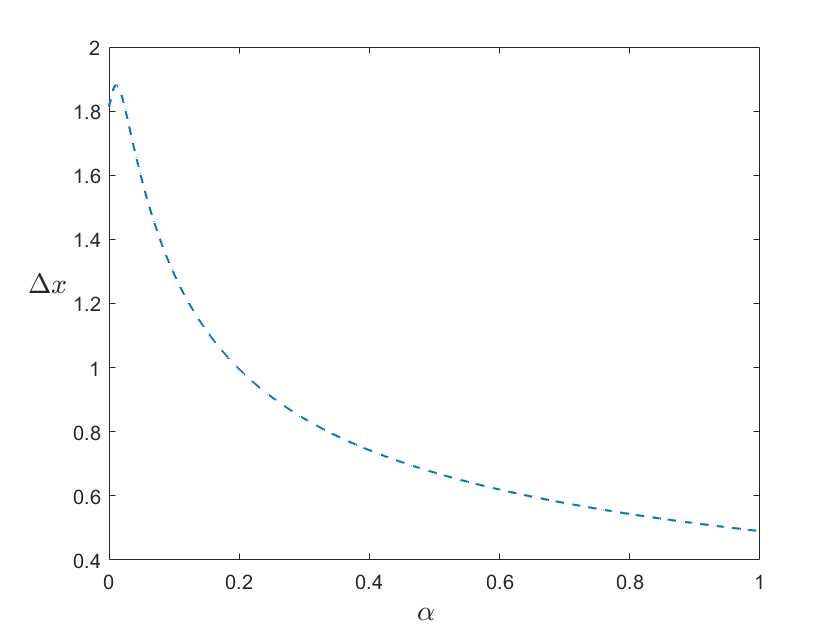
(a)

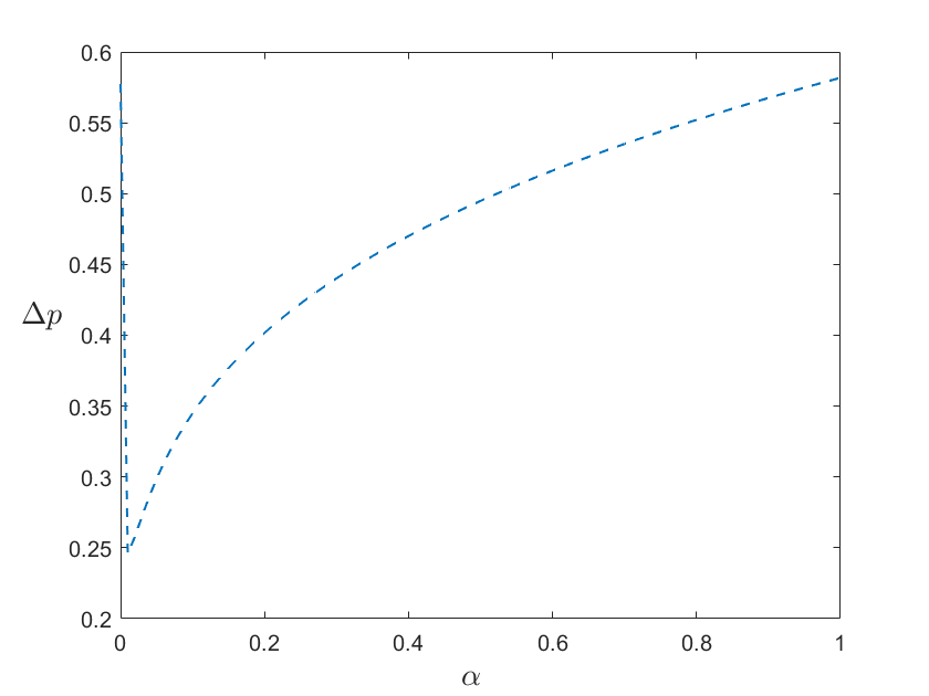
(b)

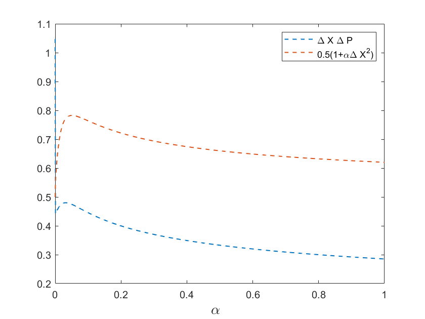
(c)

Figure 1: Bright soliton solution: (a) Position uncertainty, (b) Momentum uncertainty and (c) Extended uncertainty principle validation

For the dark soliton, unlike the ordinary case, the wave function can be normalized under the effect of the EUP. Consequently, we can establish a transcendental relation between the deformation parameter $\alpha$ and the chemical potential $\mu$ which reads:

$$\frac{\mu\pi}{2\sqrt{\alpha}}-2\sqrt{\mu}\tanh\left(\frac{\sqrt{\mu}\pi}{4\sqrt{\alpha}}\right)=1.$$ (25)

The position and momentum uncertainties of the dark soliton solution can be calculated respectively as follows

$$\Delta X=\sqrt{\int_{-\pi/(4\sqrt{\alpha})}^{\pi/(4\sqrt{\alpha})}\frac{\mu\tan^{2}(\sqrt{\alpha}\eta)\tanh^{2}(\sqrt{\mu}\eta)}{\alpha}d\eta},$$ (26)

$$\Delta P=\sqrt{-\int_{-\pi/(4\sqrt{\alpha})}^{\pi/(4\sqrt{\alpha})}\mu\tanh(\sqrt{\mu}\eta)\dfrac{\partial^{2}}{\partial\eta^{2}}\tanh(\sqrt{\mu}\eta)d\eta},$$ (27)

$\Delta X$ and $\Delta P$ along with the validation of EUP for the dark soliton solution are depicted in Fig. (2). Additionally, in Fig. 3, we have plotted the probability density.

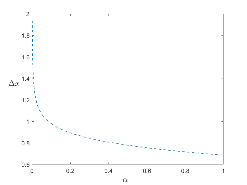
(a)

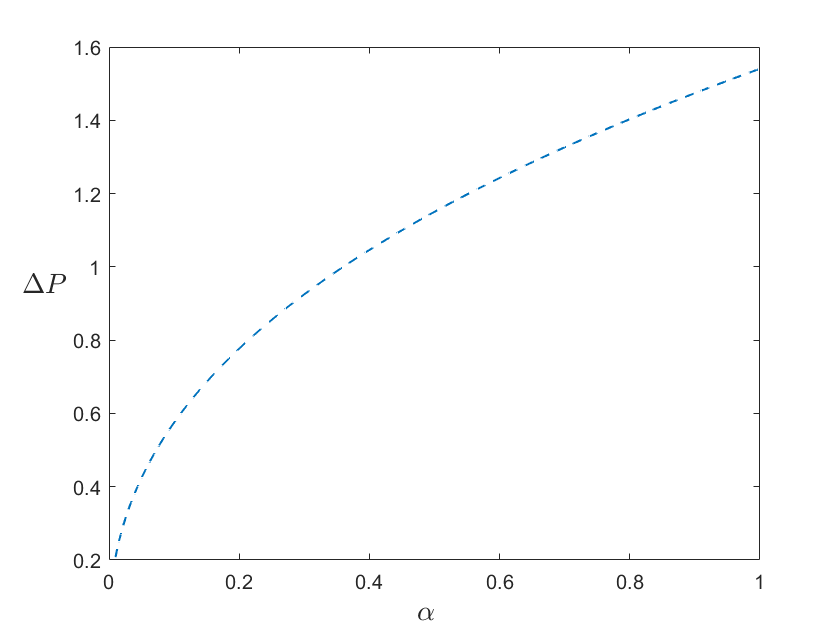
(b)

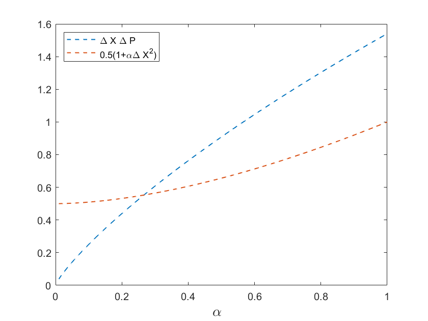
(c)

Figure 2: Dark soliton solution: (a) Position uncertainty, (b) Momentum uncertainty and (c) Extended uncertainty principle validation

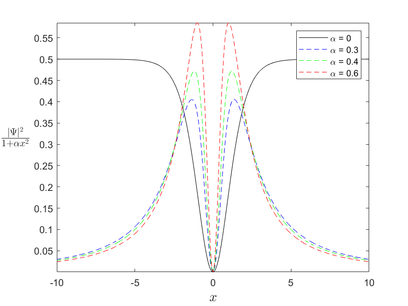
Figure 3: The profile and densities of the dark soliton solution for different values of $\alpha$

2.2 Harmonic trap

In the presence of an external potential, obtaining an exact solution to the GPE becomes intractable and challenging due to its nonlinearity nature. Thus, the focus of this section is to derive a qualitative solution for Eq. (8) subjected to a harmonic oscillator potential using the variational and validate this latter through numerical technique namely the split-step Fourier method (SSFM).

2.2.1 Variational analysis

For the harmonic oscillator (HO) potential $\displaystyle V(x)=\frac{x^{2}}{2}$ (where $\omega=1$), and utilizing the generalized momentum operator $\hat{P}=(1+\alpha x^{2})\hat{p}$, the deformed GPE takes the form:

$$i\frac{\partial\tilde{\Psi}(\eta,t)}{\partial t}=-\frac{1}{2}\frac{\partial^{2}\tilde{\Psi}(\eta,t)}{\partial\eta^{2}}+g\left\arrowvert\tilde{\Psi}(\eta,t)\right\arrowvert^{2}\tilde{\Psi}(\eta,t)+\frac{\tan^{2}(\eta\sqrt{\alpha})}{2\alpha}\tilde{\Psi}(\eta,t).$$ (28)

Here, we used $x=\tan(\sqrt{\alpha}\eta)/\sqrt{\alpha}$, this transformation converts the HO potential to Pöschl–Teller (PT) potential, which is considered a generalization of harmonic vibrators and gives phenomena such as anharmonicity. Benkrane . For stationary solution, we put

$$\tilde{\Psi}(\eta,t)=\phi(\eta)\exp(-i\mu t),$$ (29)

therefore, the effective classical field Hamiltonian for $g=-1$ is

$$H_{eff}=\int\left[\frac{1}{2}\left\lvert\frac{\partial\phi(\eta)}{\partial\eta}\right\lvert^{2}+\frac{\tan^{2}(\sqrt{\alpha}\eta)}{2\alpha}\lvert\phi(\eta)\lvert^{2}-\lvert\phi(\eta)\lvert^{4}\right]d\eta.$$ (30)

Now, we assume the following ansatz

$$\phi(\eta)=\sqrt{\frac{K}{2}}\operatorname{sech}(K\eta),$$ (31)

$K$ is a variational parameter. Taking into account the definitions (30) and(31), the effective Hamiltonian can be expressed in terms of the variational and deformation parameters as follows

$$H_{eff}=\frac{1}{8}K^{3}J_{1}+\frac{1}{4\alpha}KJ_{2}+\frac{1}{4}K^{2}J_{3}.$$ (32)

In which :

$$J_{1}=\int_{-\frac{\pi}{4\sqrt{\alpha}}}^{\frac{\pi}{4\sqrt{\alpha}}}\left(\operatorname{sech}^{2}(K\eta)-\operatorname{sech}^{4}(K\eta)\right)d\eta,$$ (33)

$$J_{2}=\int_{-\frac{\pi}{4\sqrt{\alpha}}}^{\frac{\pi}{4\sqrt{\alpha}}}\tan^{2}(\eta\sqrt{\alpha})\operatorname{sech}^{4}(K\eta)d\eta,$$ (34)

$$J_{3}=\int_{-\frac{\pi}{4\sqrt{\alpha}}}^{\frac{\pi}{4\sqrt{\alpha}}}\operatorname{sech}^{4}(K\eta)d\eta.$$ (35)

Similarly to the free case, we can compute the position and momentum uncertainties along with the validation of EUP as illustrated in Fig. (4). Furthermore, by plotting the effective Hamiltonian as a function of the variational parameters for different values of $\alpha$ (see fig. 5), we can observe that Eq. (30) displays local minima at specific values of $K$. Inserting these values into the soliton ansatz yields profiles of the bright soliton depicted in Fig. 5.

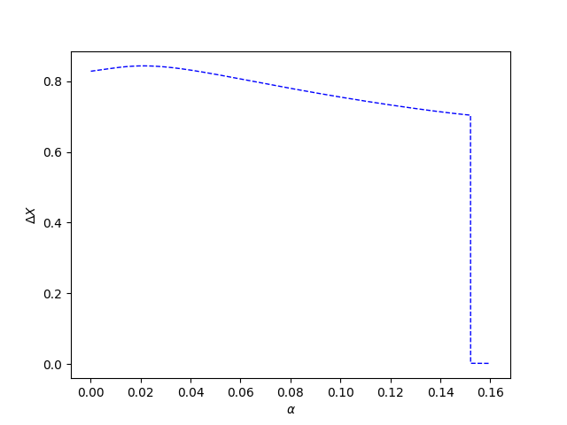
(a)

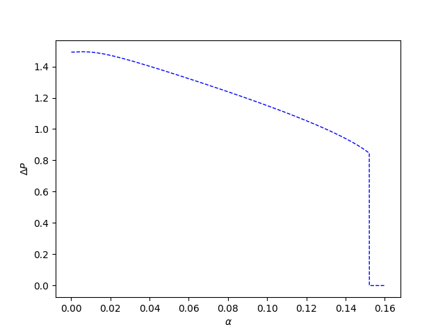
(b)

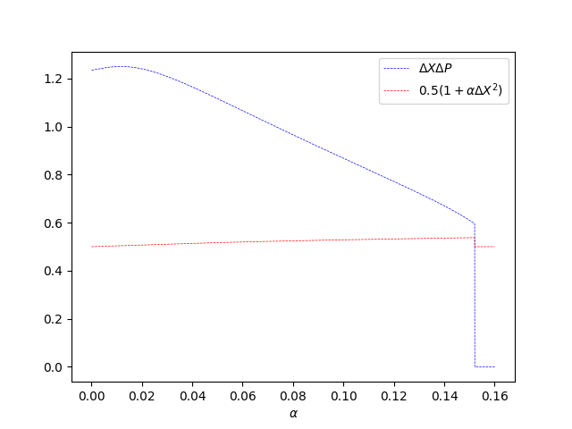
(c)

Figure 4: Variation solution of GPE in the presence of HO potential: (a) Position uncertainty, (b) Momentum uncertainty, and (c) Extended uncertainty principle validation

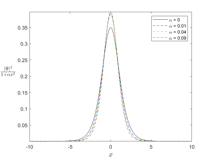
(a)

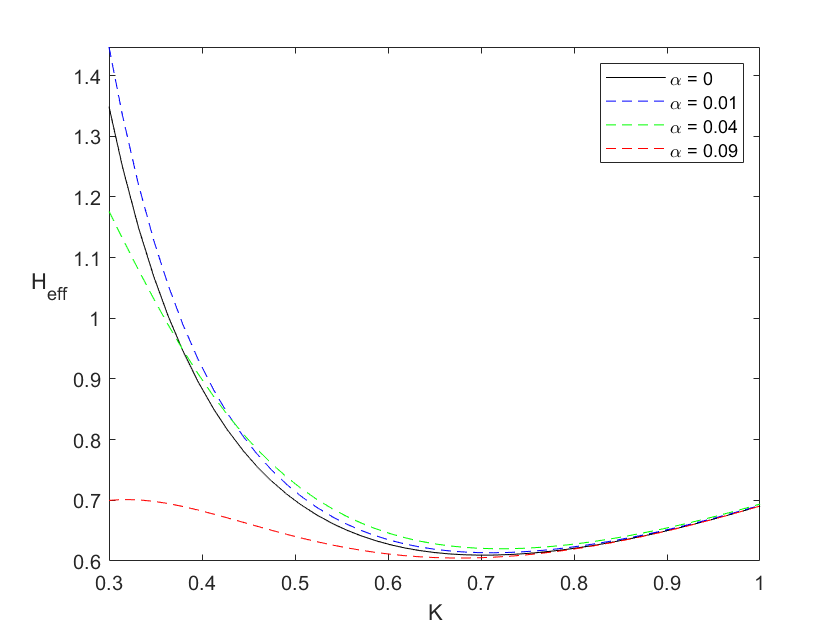
(b)

Figure 5: (a): Probability density for HO. (b): Effective Hamiltonian as a function of $K$ with different values of $\alpha$

2.2.2 Numerical analysis

The numerical solutions of Eq. (28) for various values of $\alpha$ were obtained using the split-step Fourier method (SSFM) Bao2003 , this method has proven to be a reliable approximation for the Gross-Pitaevskii equation Salman2014 ; Caliari2018 ; Wang2005 . The SSFM involves discretizing space and time and then alternating between Fourier transforming and applying evolution operators. The deformed GPE can be expressed as Bogomolov2006 :

$$i\frac{\partial\tilde{\Psi}(\eta,t)}{\partial t}=\left[\hat{\mathcal{L}}+\hat{\mathcal{N}}\right]\tilde{\Psi}(\eta,t),$$ (36)

where the linear operator $\mathcal{L}$ is defined as:

$$\hat{\mathcal{L}}=-\frac{1}{2}\frac{\partial^{2}}{\partial\eta^{2}}.$$ (37)

The nonlinear operator $\mathcal{N}$ is given by:

$$\hat{\mathcal{N}}=-\left\arrowvert\tilde{\Psi}(\eta,t)\right\arrowvert^{2}+\frac{\tan^{2}(\eta\sqrt{\alpha})}{2\alpha}.$$ (38)

Generally, $\hat{\mathcal{L}}$ and $\hat{\mathcal{N}}$ operators do not commute. However, according to the Baker-Hausdorff formula, the error introduced by treating them as if they commute is of order $(\Delta t)^{2}$ Muslu2005 ; Sinkin2003 ; Musetti2018 . Taking small time steps $\Delta t$, we can approximate the solution as follows:

$$\Psi(\mathbf{\eta},t+\Delta t)=e^{-i\hat{\mathcal{L}}\Delta t}e^{-i\hat{\mathcal{N}}\Delta t}\Psi(\mathbf{\eta},t),$$ (39)

To apply the SSFM algorithm we first compute the solution considering the part that involves the nonlinear operator.

$$\Psi(\mathbf{\eta},t+\Delta t)=e^{-i\hat{\mathcal{N}}\Delta t}\Psi(\mathbf{\eta},t)$$ (40)

In the next step, the solution (40) undergoes a transformation into the frequency domain through the application of the Fourier transformation. Subsequently, it is advanced according to the linear operator, wherein the partial derivative is converted using $ik=i\frac{\partial}{\partial\eta}$ where $k$ is the wave number. Finally, the solution is subjected to an inverse Fourier transformation. This entire process is described by the following expression:

$$\Psi(\mathbf{\eta},t+\Delta t)=\mathcal{F}^{-1}\left[e^{-i\Delta t\left(-\frac{1}{2}\mathbf{k}^{2}\right)}\mathcal{F}\left[e^{-i\hat{\mathcal{N}}\Delta t}\Psi(\mathbf{\eta},t)\right]\right],$$ (41)

in which $\mathcal{F}$ and $\mathcal{F}^{-1}$ denote the forward and inverse Fourier transforms, respectively. These steps are iteratively applied to solve Eq. (28) numerically, the code was written in MATLAB and we have taken 20000 Fourier mode with $\Delta t=0.001$, the probability densities compared to the variational solutions are depicted in Fig. (6)

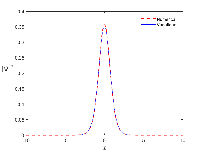
(a)

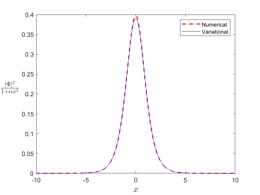
(b)

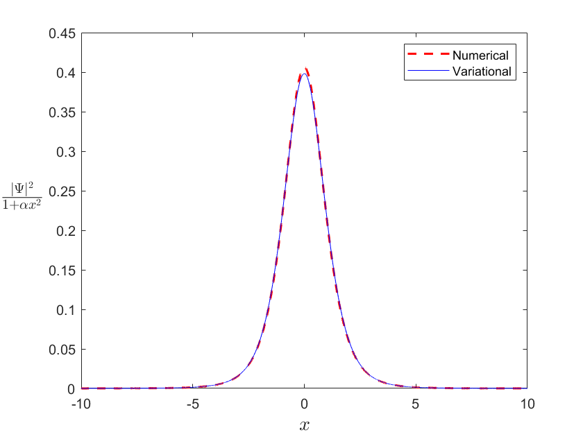
(c)

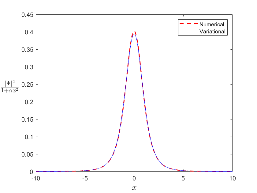
(d)

Figure 6: Numerical results compared to the variational solutions : (a) $\alpha=0$, (b) $\alpha=0.01$,
(c) $\alpha=0.04$, (d) $\alpha=0.09$

3 Discussions

We can observe the effects of EUP on the BEC by plotting the probability densities, position and momentum uncertainties for different values of deformation parameter $\alpha$. Based on the Figs. 1, 2, 3, 4, 5 and 6, we give the following perspectives :

1. In the examination of the free bright soliton solution, we have investigated the position and momentum uncertainties. The results, depicted in Fig. (1) reveal that the EUP does not apply for all values of the deformation parameter $\alpha$. Consequently, it can be asserted that, within the framework of anti-de Sitter space, the bright soliton solution does not correspond to a physical state.

2. The variations of position and momentum uncertainties with EUP validation for free dark soliton are shown in Fig. (2). It is evident that the curved space or the gravitational field enhances the precision of position measurements while concurrently diminishing the precision of momentum measurements, which leads to an increase in BEC depletion 1947 ; rev , consequently, there is a decrease in the BEC fraction 1957 ; rev . It is important to emphasize that these observations are right for the $\alpha$-values that make EUP valid and which can be extracted from Fig (2(c)), specifically starting from $\alpha\simeq 0.3$, the inequality (11) is fulfilled.

3. The Fig. (3) represents the probability density for free dark soliton with position $x$ and for different values of $\alpha$. As the EUP impact increases, the amplitude grows and the width decreases, and since the width, physically, is directly related to the position uncertainty, this confirms the decrease in the $\Delta X$ that we obtained in the fig. (2(a)).

4. The variations of position and momentum uncertainties with extended uncertainty principle validation in terms of the deformation parameter for the harmonic oscillator are illustrated in Figure (4). One can easily observe that as the $\alpha$ parameter increases, $\Delta X$ reaches a maximal value, after which the deformation parameter causes a decrease in position uncertainty. Meanwhile, the EUP directly reduces $\Delta P$, indicating a decrease in Bose-Einstein Condensate depletion and an increase in BEC fraction with space-time curvature. On the other hand, from $\alpha=0$ to $0.15<\alpha<0.155$, the EUP is valid, as depicted in Figure (4(c)).

5. The probability density and effective Hamiltonian of HO potential in the presence of EUP are presented in Fig. (5). It is worth noting that, the amplitude of probability increases with $\alpha$ and vice versa for the width. On the other hand, the effective Hamiltonian has a minimum value in terms of variational parameter $K$ for a range of the deformation parameter $\alpha\leq 0.15$, which reflects the stability of BEC. As $\alpha$ increases beyond this range, the effective Hamiltonian does not display local minima, indicating the instability of BEC.

6. The variational solutions were validated using the SSFM, the two methods show remarkable agreement; Fig. 6 with an error ranging between 0.074 and 0.077.

4 Conclusion

In this study, we explored the effects of the extended uncertainty principle on a Bose-Einstein condensate modeled by the deformed one-dimensional Gross-Pitaevskii equation. Specifically, we investigated free and harmonic trap scenarios.

Our main findings suggest that the EUP significantly influences the position and momentum uncertainties, as well as the amplitude and the width of probability density. This effect varies according to the deformation parameter $\alpha$. For instance, in the case of dark soliton, we found that the curved space increases the accuracy of measuring position and vice versa for momentum for free dark soliton, additionally, we observed the solution becomes in contrast to the ordinary case, and the gravitational effect amplifies the amplitude of the probability density.

For harmonic oscillator potential, we employed variational and numerical approaches, both approaches showed an excellent agreement. The results indicate that the anti-de Sitter space leads to an increase in the amplitude of probability density and a reduction in momentum uncertainty, which contributes to a decrease in condensate depletion and thus an increase in the condensate fraction. Finally, it is important to note that these observations for null and HO potentials are valid for certain ranges of deformation parameter $\alpha$, where the EUP inequality (11) is fulfilled.

References

- [1] Weizhu Bao, Dieter Jaksch, and Peter A Markowich. Numerical solution of the gross–pitaevskii equation for bose–einstein condensation. Journal of Computational Physics, 187(1):318–342, 2003.
- [2] Franco Dalfovo, Stefano Giorgini, Lev P Pitaevskii, and Sandro Stringari. Theory of bose-einstein condensation in trapped gases. Reviews of modern physics, 71(3):463, 1999.
- [3] N Bogoliubov. On the theory of superfluidity. J. Phys, 11(1):23, 1947.
- [4] Eugene P Gross. Hydrodynamics of a superfluid condensate. Journal of Mathematical Physics, 4(2):195–207, 1963.
- [5] Lev P Pitaevskii. Vortex lines in an imperfect bose gas. Sov. Phys. JETP, 13(2):451–454, 1961.
- [6] Aleksei Shabat and Vladimir Zakharov. Exact theory of two-dimensional self-focusing and one-dimensional self-modulation of waves in nonlinear media. Sov. Phys. JETP, 34(1):62, 1972.
- [7] A Weller, JP Ronzheimer, C Gross, J Esteve, MK Oberthaler, DJ Frantzeskakis, G Theocharis, and PG Kevrekidis. Experimental observation of oscillating and interacting matter wave dark solitons. Physical review letters, 101(13):130401, 2008.
- [8] Andrea Di Carli, Craig D Colquhoun, Grant Henderson, Stuart Flannigan, Gian-Luca Oppo, Andrew J Daley, Stefan Kuhr, and Elmar Haller. Excitation modes of bright matter-wave solitons. Physical Review Letters, 123(12):123602, 2019.
- [9] Bettina Gertjerenken, Thomas P Billam, Lev Khaykovich, and Christoph Weiss. Scattering bright solitons: Quantum versus mean-field behavior. Physical Review A, 86(3):033608, 2012.
- [10] L Salasnich, A Parola, and L Reatto. Modulational instability and complex dynamics of confined matter-wave solitons. Physical review letters, 91(8):080405, 2003.
- [11] Mariusz P Dabrowski and Fabian Wagner. Asymptotic generalized extended uncertainty principle. The European Physical Journal C, 80(7):676, 2020.
- [12] JR Mureika. Extended uncertainty principle black holes. Physics Letters B, 789:88–92, 2019.
- [13] A Merad, M Aouachria, M Merad, and Tolga Birkandan. Relativistic oscillators in new type of the extended uncertainty principle. International Journal of Modern Physics A, 34(32):1950218, 2019.
- [14] Abdelhakim Benkrane and Hadjira Benzair. The thermal properties of a two-dimensional dirac oscillator under an extended uncertainty principle: path integral treatment. The European Physical Journal Plus, 138(3):1–16, 2023.
- [15] B Hamil, M Merad, and Tolga Birkandan. Pair creation in curved snyder space. International Journal of Modern Physics A, 35(04):2050014, 2020.
- [16] B Hamil, M Merad, and Tolga Birkandan. The duffin-kemmer-petiau oscillator in the presence of minimal uncertainty in momentum. Physica Scripta, 95(7):075309, 2020.
- [17] A Merad, M Aouachria, and H Benzair. The eup dirac oscillator: A path integral approach. Few-Body Systems, 61(4):36, 2020.
- [18] Raimundo N Costa Filho, João PM Braga, Jorge HS Lira, and José S Andrade Jr. Extended uncertainty from first principles. Physics Letters B, 755:367–370, 2016.
- [19] Jaume Giné and Giuseppe Gaetano Luciano. Modified inertia from extended uncertainty principle (s) and its relation to mond. The European Physical Journal C, 80:1–8, 2020.
- [20] E Castellanos and JI Rivas. Planck-scale traces from the interference pattern of two bose-einstein condensates. Physical Review D, 91(8):084019, 2015.
- [21] Mahnaz Maleki, Hosein Mohammadzadeh, and Zahra Ebadi. Nonextensive gross pitaevskii equation. International Journal of Geometric Methods in Modern Physics, 20(12):2350216–330, 2023.
- [22] Frank Wilczek. Anyons. Scientific American, 264(5):58–65, 1991.
- [23] Frank Wilczek. Disassembling anyons. Physical review letters, 69(1):132, 1992.
- [24] Behrouz Mirza and Hosein Mohammadzadeh. Thermodynamic geometry of fractional statistics. Physical Review E, 82(3):031137, 2010.
- [25] Manjun Ma and Zhe Huang. Bright soliton solution of a gross–pitaevskii equation. Applied Mathematics Letters, 26(7):718–724, 2013.
- [26] Jesus Rogel-Salazar. The gross–pitaevskii equation and bose–einstein condensates. European Journal of Physics, 34(2):247, 2013.
- [27] Salvatore Mignemi. Extended uncertainty principle and the geometry of (anti)-de sitter space. Modern Physics Letters A, 25(20):1697–1703, 2010.
- [28] Brett Bolen and Marco Cavaglia. (anti-) de sitter black hole thermodynamics and the generalized uncertainty principle. General Relativity and Gravitation, 37:1255–1262, 2005.
- [29] Manjun Ma, Chi Dang, and Zhe Huang. Analytical expressions for dark soliton solution of a gross–pitaevskii equation. Applied Mathematics and Computation, 273:383–389, 2016.
- [30] Latévi M Lawson, Prince K Osei, Komi Sodoga, and Fred Soglohu. Path integral in position-deformed heisenberg algebra with maximal length uncertainty. Annals of Physics, page 169389, 2023.
- [31] Kourosh Nozari and Amir Etemadi. Minimal length, maximal momentum, and hilbert space representation of quantum mechanics. Physical Review D, 85(10):104029, 2012.
- [32] Weizhu Bao, Dieter Jaksch, and Peter A. Markowich. Numerical solution of the gross–pitaevskii equation for bose–einstein condensation. Journal of Computational Physics, 187(1):318–342, May 2003.
- [33] Hayder Salman. A time-splitting pseudospectral method for the solution of the gross–pitaevskii equations using spherical harmonics with generalised-laguerre basis functions. Journal of Computational Physics, 258:185–207, February 2014.
- [34] M. Caliari and S. Zuccher. Reliability of the time splitting fourier method for singular solutions in quantum fluids. Computer Physics Communications, 222:46–58, January 2018.
- [35] Hanquan Wang. Numerical studies on the split-step finite difference method for nonlinear schrödinger equations. Applied Mathematics and Computation, 170(1):17–35, November 2005.
- [36] Ya.l. Bogomolov and A.D. Yunakovsky. Split-step fourier method for nonlinear schrodinger equation. In DAYS on DIFFRACTION 2006. IEEE, 2006.
- [37] G.M. Muslu and H.A. Erbay. Higher-order split-step fourier schemes for the generalized nonlinear schrödinger equation. Mathematics and Computers in Simulation, 67(6):581–595, January 2005.
- [38] O.V. Sinkin, R. Holzlohner, J. Zweck, and C.R. Menyuk. Optimization of the split-step fourier method in modeling optical-fiber communications systems. Journal of Lightwave Technology, 21(1):61–68, January 2003.
- [39] Simone Musetti, Paolo Serena, and Alberto Bononi. On the accuracy of split-step fourier simulations for wideband nonlinear optical communications. Journal of Lightwave Technology, 36(23):5669–5677, December 2018.
- [40] N Bogoliubov. On the theory of superfluidity. J. Phys, 11(1):23, 1947.
- [41] Raphael Lopes, Christoph Eigen, Nir Navon, David Clément, Robert P Smith, and Zoran Hadzibabic. Quantum depletion of a homogeneous bose-einstein condensate. Physical review letters, 119(19):190404, 2017.
- [42] Raphael Lopes, Christoph Eigen, Nir Navon, David Clément, Robert P Smith, and Zoran Hadzibabic. Quantum depletion of a homogeneous bose-einstein condensate. Physical review letters, 119(19):190404, 2017.