Feature Map Testing for Deep Neural Networks

Abstract

Due to the widespread application of deep neural networks (DNNs) in safety-critical tasks, deep learning testing has drawn increasing attention. During the testing process, test cases that have been fuzzed or selected using test metrics are fed into the model to find fault-inducing test units (e.g., neurons and feature maps, activating which will almost certainly result in a model error) and report them to the DNN developer, who subsequently repair them (e.g., retraining the model with test cases). Current test metrics, however, are primarily concerned with the neurons, which means that test cases that are discovered either by guided fuzzing or selection with these metrics focus on detecting fault-inducing neurons while failing to detect fault-inducing feature maps.

In this work, we propose DeepFeature, which tests DNNs from the feature map level. When testing is conducted, DeepFeature will scrutinize every internal feature map in the model and identify vulnerabilities that can be enhanced through repairing to increase the model’s overall performance. Exhaustive experiments are conducted to demonstrate that (1) DeepFeature is a strong tool for detecting the model’s vulnerable feature maps; (2) DeepFeature’s test case selection has a high fault detection rate and can detect more types of faults (comparing DeepFeature to coverage-guided selection techniques, the fault detection rate is increased by 49.32%). (3) DeepFeature’s fuzzer also outperforms current fuzzing techniques and generates valuable test cases more efficiently.

I Introduction

Deep neural networks (DNNs) are widely used in safety-critical domains, such as autonomous driving [1] and medical diagnosis [2]. However, DNNs can be complex and susceptible to data bias, overfitting, and underfitting, making them far from dependable for these applications. To address this problem, DNNs must undergo deep learning testing techniques before deployment to ensure their reliability [3, 4]. This testing helps identify and repair units (e.g., neurons and feature maps) in the model that are particularly vulnerable to change and can significantly impact the model’s performance, resulting in a more reliable model.

The deep learning testing technique mainly has three key elements: coverage metric, test case selection, and fuzzing strategy. The testing process typically works in an iterative way. In each iteration, the testing techniques will first feed test cases, which are selected or fuzzed with certain rules (e.g., coverage metric), into the model, after which a coverage metric is calculated. New test cases will be generated to further improve the coverage metric until the metric meets the developers’ requirements.

The most important element mentioned above is the coverage metric since it determines how test cases are generated (i.e., fuzzed or selected from a massive amount of candidate test sets) to reveal the fault-inducing units (e.g., neuron and feature map. Illustrated in Fig. 1) of a tested DNN. Therefore, the main criterion of coverage metrics is to explore as much diversity as possible of a certain subspace defined based on different abstraction levels (e.g., neuron activation [3], neuron activation pattern [4], and neuron activation conditions [5]), while test case selection and fuzzing strategy are used to obtain new test cases, which are fed into the model to increase coverage metrics. To explore more types of model units’ behaviors, multiple Neuron Coverage (NC) metrics, including NAC [3], KMNC [4], IDC [6], and MC/DC [7] have been proposed.

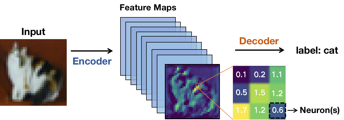
Figure 1: An illustration of feature maps and neurons. A neuron is a basic unit of computation in a neural network. A feature map is a set of neurons that are connected to the same input and that together produce an output that encodes certain features (e.g., color, and texture).

Key problems of existing NC-guided testing. Despite the fact that existing NC-guided testing techniques have greatly advanced deep learning testing, there remains a significant constraint, namely that not all fault-inducing units in the model are neurons. Recent studies [8, 9] have revealed that feature maps are also important fault-inducing units that can affect DNN performance, while NC-guided techniques often focus on analyzing neuron’s behavior and fail to capture and utilize feature-map-level information, causing DNN developers can not detecting feature maps that induce errors. Consequently, NC-guided testing techniques yield a sub-optimal fault detection rate and can merely bring a significant boost to the model [10, 11], as retraining the model with test cases generated by NC-Fuzz (e.g., DeepXplore [3], DeepHunter [12], and ADAPT [13]) can only repair fault-inducing neurons.

In this work, we address this problem by proposing DeepFeature, which test DNNs from feature map level. As opposed to heuristically defining various neuron-level metrics, we establish a clear connection between output variation at the feature-map level and the performance of the model through clear experiments. As illustrated in Fig. 1, the main distinction between DeepFeature and existing neuron coverage testing works is that DeepFeature tests the DNN model from the feature-map level. Specifically, during the testing process, DeepFeature delves into every inner feature map in the model to evaluate its vulnerability. The vulnerable feature maps therein are then repaired by retraining with test cases selected or generated using our corresponding selection and fuzzing strategy while further improving the overall performance of the model.

To validate the effectiveness of DeepFeature, we conduct experiments with four popular DNN models across four widely-used datasets. The experiment results validate our motivation and demonstrate the superiority of our method. Specifically, in comparison to state-of-the-art neuron-level test case selection methods, our DeepFeature yields a higher fault detection rate (e.g., DeepFeature maximum increases 49.32% fault detection rate compared with NC-guided baselines), and in limited test case selection scenarios, DeepFeature can detect more type of faults that are ignored by baselines. DeepFeature’s Fuzzer is further exhibited to be the most effective and efficient among state-of-the-art fuzzing techniques.

In a nutshell, we make the following contributions.

• We propose a novel set of testing metrics to quantify the feature map’s vulnerability.

• We propose a new selection method that can productively select test cases with a high probability of fooling the model from a massive number of unlabeled test cases (e.g., DeepFeature maximum increases 49.32% fault detection rate compared with NC-guided baselines).

• We propose feature-map-guided fuzzing technique that outperforms current fuzzing techniques.

II Background

This section includes several basic knowledge of neural networks, neuron coverage metrics, test case selection, and fuzzing strategies.

II-A Neuron, Feature Map and Neural Network

In this work, we focus on deep learning models (e.g., deep neural networks) for classification, which can be presented as a complicated function $f:\mathcal{X}\rightarrow\mathcal{Y}$ mapping an input $x\in\mathcal{X}$ into a label $y\in\mathcal{Y}$. Unlike traditional software, programmed with deterministic algorithms by developers, DNNs are defined by the training data, along with the network structures.

As shown in Fig. 1, neurons and feature maps are fundamental concepts in the field of deep neural networks (DNNs), which have emerged as powerful tools for image recognition and other tasks involving large amounts of data. A neuron is a basic unit of computation in a neural network. It receives input from other neurons or from the input layer, applies a set of weights and biases to this input, and then applies an activation function to produce an output, where the activation function is a mathematical function that determines the output of a neuron based on its input. Common activation functions include Sigmoid, Tanh, and ReLU. A feature map, on the other hand, is a set of neurons that are connected to the same input and that together produce an output that encodes certain features or patterns in the input. In a DNN, multiple feature maps are typically stacked together to form a hierarchy of features, with lower-level feature maps encoding simpler patterns and higher-level feature maps encoding more complex patterns.

The main difference between neurons and feature maps is that neurons are individual units of computation, whereas feature maps are collections of neurons that work together to extract specific features from the input. Neurons are the building blocks of a DNN, whereas feature maps are the building blocks of the DNN’s ability to recognize patterns in the input data.

II-B Neuron Coverage Metrics

Neuron Activation Coverage (NAC($k$))

NAC($k$) was proposed by DeepXplore [3], NAC($k$) assumes that the more neurons are activated, the more states of DNN are explored. The parameter $k$ of this coverage criteria is defined by the developer to specify how a neuron in a DNN can be counted as covered (i.e., if the output of a neuron is large than $k$, the developer will take the neuron as covered). The rate of NAC($k$) for a test is defined as the ratio of the number of covered neurons to the total number of neurons.

K-multisection Neuron Coverage (KMNC($k$))

Based on the NAC($k$) assumption about the DNN states, DeepGuage [4] further partitions the neuron’s output into $k$ ranges (e.g., 2000), and each range represents one state in DNN. Specifically, suppose that the output of a neuron $N$ on the training set is in the interval $[low_{N},high_{N}]$, and divide them equally into $k$ segments.

II-C Test Case Selection Methods

In this section, we introduce several widely used test case selection methods, which are used to select valuable test cases from a massive number of datasets. Specifically, the goal of the test case selection method is to sampler a fixed size ($N$) subset $I_{N}$ from the total test set $I_{T}$. We divide test case selection methods into two types: coverage-guided test case selection and prioritization test case selection.

II-C1 Coverage-guided test case selection

Coverage-guided (e.g., NAC) selection methods try to select test cases that can reach maximum coverage metrics and lead to a higher fault detection rate [3, 14, 4].

II-C2 Prioritization test case selection

Generally, for a given total test set $I_{T}$, prioritization test selection methods compute a probability $p_{i}$ for each test case $i$ in the total test set. The value of $p_{i}$ represents the probability of test case $i$ sampled by selection methods.

II-D Fuzzing Strategies

DeepXplore [3] is the first DNN testing framework. It proposes a neuron activation coverage (NAC) guided fuzzing strategy to increase the neuron activation coverage metric. Inspired by DeepXplore,  Hu et al. [15] propose DeepMutation++ [15], which generates test cases to increase multi-granularity coverage metrics. Inspired by DeepXplore, and DeepMutation++,  Lee et al. [13] propose ADAPT, which integrates multiple neuron behaviors  (e.g., NAC and TKNC) to fuzz test cases.

Dataset	DNN Model	Neurons	Layers	Ori Acc (%)
MNIST [16]	LeNet-1 [17]	3,350	5	89.50
	LeNet-5 [17]	44,426	7	91.79
CIFAR-10 [18]	ResNet-20 [19]	543,754	20	86.07
	VGG-16 [20]	35,749,834	21	82.52
Fashion [21]	LeNet-1 [17]	3,350	5	78.99
	ResNet-20 [19]	543,754	20	86.12
SVHN [22]	LeNet-5 [17]	44,426	7	84.17
	VGG-16 [20]	35,749,834	21	92.02

TABLE I: Datasets and DNNs for evaluating DeepFeature.

III Methodology

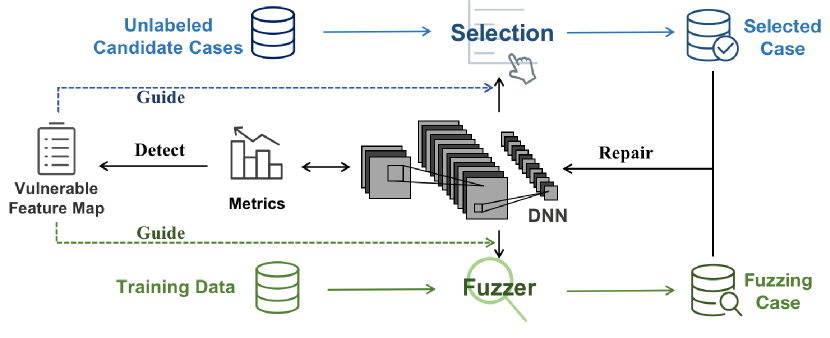
Figure 2: Overview of DeepFeature’s framework.

III-A Motivation

Deep Neural Networks (DNNs) are known to be sensitive to any perturbations in their parameters, leading to vulnerabilities in certain units (e.g., neurons or feature maps), making them more susceptible to perturbations [23, 3, 12]. Deep learning testing aims to discover these vulnerable units and repair them to make the model more reliable. Traditional deep learning testing has only considered the vulnerability of neurons by generating test cases to vary certain neurons’ status and see if a DNN produces wrong labels, but recent studies [9, 8] have shown that without altering any neuron’s status, feature maps (sets of neurons) can also lead to wrong DNN output and thus become vulnerable. Therefore, a feature map may not contain any vulnerable neurons but can still be vulnerable and cause a significant impact on the model’s performance.

Unfortunately, current neuron testing techniques are not equipped to detect vulnerable feature maps due to a lack of proper metrics, evaluation methods for vulnerable feature maps, and testing techniques designed to detect vulnerable feature maps. Existing coverage metrics for deep learning testing are based on neurons, and there are no methods to evaluate the vulnerability of a feature map. As a result, there is a pressing need for a comprehensive testing approach that addresses these limitations.

In this section, we address above-mentioned problem by proposing DeepFeature, a novel feature-map-level testing technique for deep neural networks. DeepFeature can detect vulnerable feature maps in a DNN and repair them. The overall framework of DeepFeature is shown in Fig. 2. For ease of discussion, this section defines the following notations for DNNs and feature maps: $f_{\theta}$ is a DNN parameterized by $\theta$, and there are $C$ channels (i.e., $C$ different feature maps) in the model. The $c$-th feature map in the DNN is denoted as $f_{\theta}^{c}$. $f_{\theta}^{c}(x)$ denotes the output of the corresponding feature map when the network input is $x$.

III-B Feature Map Attack

We first propose the prototype of Feature Map Attack (FMA), which is used to generate mutation cases for a given model’s feature map and test cases. The FMA algorithm, shown in Algorithm 1, iteratively generates mutated samples and maximizes the difference between the feature maps of the mutated cases and the original test cases. Specifically, the algorithm first initializes each test case with added random noise and then performs a specified number of iterations, using a gradient-based optimization method to maximize the difference between the feature maps of the mutated cases and the original test cases. In our algorithm, we add a clamping function to ensure that the perturbations stay within a certain range. We also set the number of iterations as $steps$ while the parameter $\epsilon$ controls the strength of the perturbations.

1

Input: $f_{\theta}^{c}$: model’s feature map to be tested; $x$: test case (clean sample); $\alpha$: step size; $\epsilon$: maximum perturbation; $steps$: mutation steps;

2

output :  $x^{\prime}$: mutation case (adversarial sample).

3

4Function $\text{FMA}(f_{\theta}^{c},x,steps,\alpha,\epsilon)$:

5      

6      Initialize: $x^{{}^{\prime}}\leftarrow x+\text{random\_noise}$;

7      

8      for $step=1$ to $steps$ do

9             $loss\leftarrow\|f_{\theta}^{c}(x)-f_{\theta}^{c}(x^{\prime})\|^{2}$;

10            

11            $grad\leftarrow\frac{\partial loss}{\partial x^{\prime}}$;

12            

13            $x^{{}^{\prime}}\leftarrow x^{{}^{\prime}}+\alpha\cdot\text{sign}(grad)$;

14            

15            $\delta\leftarrow\text{clamp}(x^{{}^{\prime}}-x,-\epsilon,\epsilon)$;

16            

17            $x^{{}^{\prime}}\leftarrow\text{clamp}(x+\delta,0,1)$;

18            

19      

20      return $x^{\prime}$

Algorithm 1 Feature Map Attack

III-C Feature map Attack Score

The attack success rate of DNNs under FMA against different feature maps can vary greatly. Generally, different feature maps in a DNN have different vulnerabilities, and their impact on model attack success rate is also different. Therefore, we propose Feature map Attack Score (FAS) to measure the effect of different feature maps on model performance. The FAS for the $c$-th feature map is defined as the attack success rate of the DNN when the $c$-th feature map is attacked by FMA. Specifically for the $c$-th feature map in the model. $FAS(f_{\theta}^{c},\mathcal{X})$ is defined as:

$$FAS(f_{\theta}^{c})=1-\frac{\sum_{i=0}^{N}\mathbb{I}(f_{\theta}(x_{i}^{\prime})==y_{i})}{\sum_{i=0}^{N}\mathbb{I}(f_{\theta}(x_{i})==y_{i})}$$

Where $\mathcal{X}=\{x_{i}\mid i=1,2,\dots,N\}$ is the developer provided test cases, $\{y_{i}\mid i=1,2,\dots,N\}$ is its ground-truth label and the mutation samples $\{x_{i}^{\prime}\mid i=1,2,\dots,N\}$ is generated by FMA based on the feature map $f_{\theta}^{c}$ (i.e., for different feature map, FMA will generate different mutation samples). The FAS for a feature map ranges between 0 and 1, where the value of 0 means that using FMA to attack the feature map will not affect the performance of the DNN, which indicates the feature map is not vulnerable. The value of 1 means that using FMA to attack the feature map has a significant effect on the performance of the DNN, and the larger the FAS value means the feature map is more vulnerable than others.

Feature Map	FMA steps
Index	3	7	10	20
1	58.85	68.73	68.65	67.72
2	35.15	44.09	44.11	43.07
3	3.45	3.72	3.70	3.91
4	48.26	60.98	59.29	62.81
5	32.90	42.42	42.74	41.09
6	56.68	66.07	66.93	66.39

TABLE II: A example of FAS in LeNet5 pretrained model

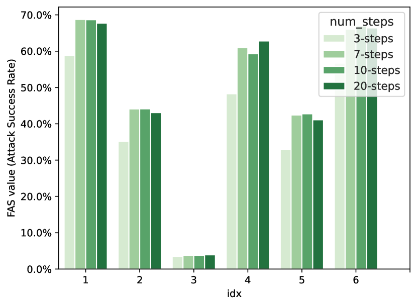
(a) SVHN&LeNet-5

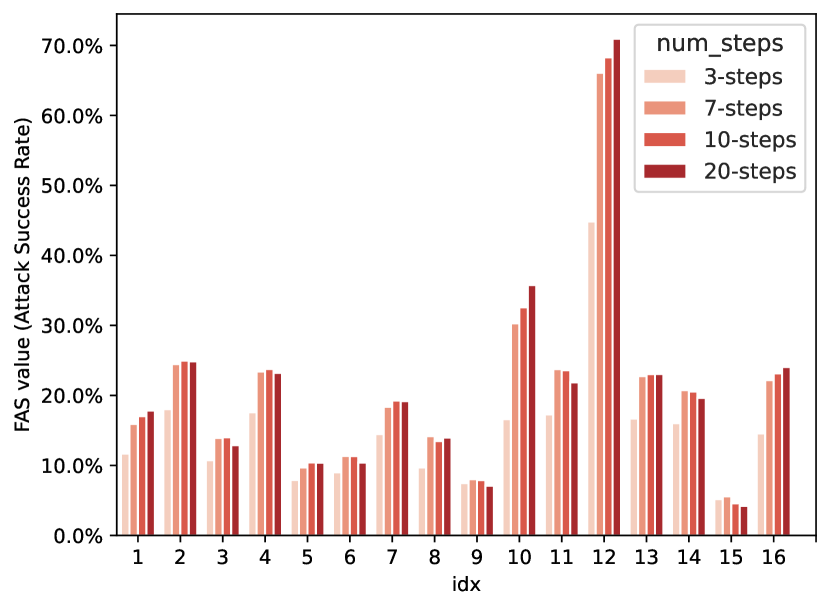
(b) CIFAR10&ResNet-20

Figure 3: Different feature maps’ vulnerability. The x-axis is the index of the feature maps, and the y-axis is the FAS value (attack success rate). A larger FAS value indicates a more vulnerable feature map.

Example 1.

Here we first take a SVHN & LeNet5 pre-trained model as an example to illustrate the FAS introduced above. For the pre-trained model, there are 6 different feature maps in the first layer. Then we feed the labeled dataset $\mathcal{X},\mathcal{Y}$ into the FMA with each feature map. FAS results are shown in Tab. II, we can observe that for different feature maps in the model’s first layer, the FAS will be largely different. For instance, the 3th feature map is the most robust compared with other feature maps, which obtain low FAS for different attack strengths. In contrast, the 1st and 6th feature maps are vulnerable to even a 3-step FMA attack, which indicates that the 1st and 6th feature maps are vulnerable and that the DNN developers need to enhance them to avoid errors in safety-critical scenarios. Then we further illustrate other combinations to evaluate the feature map’s vulnerability. As shown in Fig. 3, the distribution of FAS is consistent across different strengths of the FMA, datasets, and models, indicating that the vulnerability of feature maps is an intrinsic characteristic of pre-trained models. Additionally, the experiment results reveal that there are particularly vulnerable feature maps among those learned in a layer of the model (e.g., the 12th feature map in Fig. 3(b)), attacking it can easily cause the model has incorrect behavior. These feature maps are what DNN developers need to pay extra attention to, as test cases that can induce these feature maps into error can more easily cause the model to misclassify.

Feature Map	Mutation Strength
Index	I	II	III	IV
1	4.88e-4	1.93e-3	4.29e-3	7.52e-3
2	1.89e-4	7.34e-4	1.58e-3	2.70e-3
3	4.97e-8	1.91e-7	4.16e-7	7.40e-7
4	2.39e-4	9.31e-4	2.03e-3	3.52e-3
5	1.83e-4	7.33e-4	1.64e-3	2.91e-3
6	3.16e-4	1.26e-3	2.81e-3	4.96e-3

TABLE III: A example of FVS in LeNet5 pre-trained model

(a) SVHN&LeNet-5

(b) CIFAR10&ResNet20

Figure 4: FVS value of different feature maps. The darker the color indicates the greater the degree of data perturbation, which is aligned with Fig. 3. We use mutation to generate test cases here to be consistent with the selection experiment. Mutation refers to benign augmentation, whose strength is increased by increasing augmentation parameters’ value range (as mentioned in Tab. IV).

Input: $x\in\mathcal{X}:\text{original test cases}\;x^{\prime}\in\mathcal{X^{\prime}}:\text{benign mutation test cases}\;f_{\theta}:\text{DNN to be tested}\;N:\text{The number of test cases to be selected}\;K:\text{TopK vulnerable feature map}$

output : $\mathcal{X_{s}}$: selected test cases

1

2Function FVS-Selection($f_{\theta}$, $\mathcal{X}$, $\mathcal{X}^{\prime}$, $N$, $K$):

       /* Detect TopK Vulnerable Feature Map */

3       $FM$: Initialize vulnerable feature map list

4       $FM\leftarrow f_{\theta}[\text{argsort}(\{FVS(f_{\theta}^{c})\}_{\text{for each }}f_{\theta}^{c}\in f_{\theta})][-K:]$

       /* Test Case Selection Begins */

5       $FVS\_array=[]$

6       for each $x_{i},x_{i}^{\prime}in\mathcal{X},\mathcal{X}^{\prime}$ do

7             $FM\_score=0$

8            

9            for each $f_{\theta}^{c}\in FM$ do

10                   $FM\_score+=FVS(f_{\theta}^{c}(x_{i}),f_{\theta}^{c}(x_{i}^{\prime}))$

11            $FVS\_array.append(FM\_score)$

12      $\mathcal{X_{s}}=\mathcal{X}[\text{argsort}(FVS\_array)][-N:]$

13       return $\mathcal{X_{s}}$

Algorithm 2 Test Case Selection Pipeline

III-D Feature map Vulnerability Score

As discussed in Sec. III-C, FAS will need the ground-truth label to calculate the score, which means once the developers only have unlabelled data, they can not use FAS to detect vulnerable feature maps. To solve this problem, we introduce FVS, another metric to detect vulnerable feature maps which measures the feature maps’ vulnerability by directly computing the feature map output’s difference between the test cases and its mutation examples (i.e., feature map output’s difference between $x$ and $x^{\prime}$). Formally, given a feature map $f_{\theta}^{c}$ in the model, a test set $\mathcal{X}=\{(x_{i})\mid i=1,2,\dots,N\}$ and its corresponding mutated test set $\mathcal{X}^{\prime}=\{(x_{i}^{\prime})\mid i=1,2,\dots,N\}$ generated by a user-defined mutation method (e.g., rotation, shear, blur, and FMA), the FVS is defined as:

$$FVS(f_{\theta}^{c})=\frac{1}{N}\sum_{i=0}^{N}(\|f_{\theta}^{c}(x)-f_{\theta}^{c}(x^{\prime})\|^{2})$$

where $f_{\theta}^{c}(x_{i})$ is the output of $x_{i}$ in the $c$-th feature map of the model $f_{\theta}$. The FVS for a feature map ranges between 0 and $\infty$, where a value of 0 means that the feature map will not be affected by the perturbation, which indicates that this feature map is not vulnerable. A value large than 0 means it will be affected by the perturbation, and the larger FVS for the feature map, the more vulnerable it is.

Example 2.

In this part, we take the same SVHN & LeNet5 pre-trained model as in Sec. III-C to illustrate the effectiveness of FVS introduced above. Specifically, for dataset $\mathcal{X}$ we use mutation methods in Tab. IV to generate $\mathcal{X^{\prime}}$, then we feed these cases into the model to calculate the FVS for each feature maps in the first layer. Results are shown in Tab. III, we can observe that the 3rd feature map has low FVS value, while the 1st and 6th have high FVS values, which means the 3rd feature map is robust while the 1st and 6th are vulnerable for the perturbation. Observations are consistent with the Tab. II, indicating the interchangeability between FVS and FAS in label-agnostic scenarios. Then we further illustrate other combinations to evaluate the FVS. Results shown in Fig. 4, FVS effectively captures the most vulnerable feature maps in the model. We find that FVS and FAS have the same distribution under the same model, which means we can use FVS to replace FAS in label-agnostic scenarios (i.e., unlabeled dataset).

Input: $f_{\theta}$: pretrained DNN model, $x\in\mathcal{X}$: test cases; $\epsilon$: the fuzzing boundary, $\alpha$: and fuzzing step size, $steps$: the maximum number of steps to fuzz for a test case, $K$: TopK vulnerable feature map

output : $\mathcal{X_{s}}$: fuzzing cases generated by FMA-Fuzzer

1 Function FMA-Fuzzer($f_{\theta}$,$\mathcal{X}$,$\epsilon$,$\alpha$,$steps$,$K$):

       /* Detect TopK Vulnerable Feature Map */

2      

3      $FM$: Initialize vulnerable feature map list

4      $FM\leftarrow f_{\theta}[argsort([FVS(f_{\theta}^{c})\ for\ each\ f_{\theta}^{c}\in f_{\theta}])[-K:]]$

      /* FMA-Fuzzer Begins */

5       for each $x\in\mathcal{X}$ do

6             for each $f_{\theta}^{c}\in FM$  do

7                   $x^{\prime}=FMA(f_{\theta}^{c},x,steps,\alpha,\epsilon)$ if $f_{\theta}(x^{{}^{\prime}})!=y$ then

8                         $\mathcal{X_{s}}$.append($x^{{}^{\prime}}$)

9                  

10            

11      return $\mathcal{X_{s}}$

Algorithm 3 Fuzzer Pipeline

III-E Enhancing the DNN with DeepFeature

III-E1 Test Case Selection From Unlabeled Data

Both testing and repairing the DNN-driven system rely on manually labeled data. While collecting a massive amount of unlabeled data is usually easy to achieve, the cost of manual labeling is much greater. For data with strong expertise knowledge (e.g., medical data), it is unrealistic to blindly label all collected data. Therefore, DNN test case selection is crucial to select valuable data, reducing the labeling cost.

To select valuable test cases from unlabeled data, we propose a FVS-guided test case selection method, which select test cases with high FVS value. Algo 2 demonstrates the workflow of our FVS-guided test case selection. Specifically, we first feed the unlabeled test cases and its benign mutation cases into the $FVS-Selection()$, then we will use $\mathcal{X}$ and $\mathcal{X}^{\prime}$ to obtain the vulnerable feature map list (Algo 2 line 3). After obtain the vulnerable feature map list, we will begin to select test cases. For each input $x$ and its mutation case $x^{\prime}$, we will calculate the $FM\_score$ and then return the $\mathcal{X_{s}}$ that have larger $FM\_score$ than others.

III-E2 Data augmentation by Fuzzing

Another important application of DeepFeature is to generate data to increase the dataset capacity when the dataset is limited. Specifically, as one of the main elements for training DNN models, the dataset’s size seriously affects the trained model’s performance. We apply DeepFeature to the data augmentation task to solve this problem by using our FMA-Fuzzer to expand the dataset. Algorithm 3 presents the details of our proposed FMA-Fuzzer. The inputs include the model $f_{\theta}$, the original test cases $\mathcal{X}$, the fuzzing boundary $\epsilon$, the maximum number of steps to fuzz for a test case $step$, and fuzzing step size $step\_size$. For each test case $x\in\mathcal{X}$, FMA-Fuzzer generates multiple samples corresponding to multiple vulnerable feature maps (Alg 3). Specifically, for each test case $x$, we iteratively generate perturbations targeting each feature map by maximizing the FVS value (Alg 3 line 5-9). We first add a random perturbation to generate the initial $x^{{}^{\prime}}$ as the first step. As we need to make sure the $loss$, formulated as:

$$loss=FVS(f_{\theta}^{c}(x^{\prime}),f_{\theta}^{c}(x))$$

starts at a non-zero value to obtain a non-zero gradient. The generated sample will be then added to the fuzzing list $\mathcal{X_{s}}$ if the model misclassifies it.

IV Evaluation

We evaluate DeepFeature and answer the following research questions.

• RQ1: How effective is DeepFeature’s test case selection?

• RQ2: How effective is DeepFeature’s fuzzing algorithm?

• RQ3: Can DeepFeature behave stable under different settings?

IV-A Experiment Setup

Datasets and Models.

We adopt four widely used image classification benchmark datasets for the evaluation (i.e., MNIST [16], Fashion MNIST [21], SVHN [24], and CIFAR10 [18]), which are most commonly used datasets in deep learning testing [3, 15, 25, 4, 12, 26, 14, 6, 10, 13, 27, 23]. Table I presents the detail of the datasets and models. The MNIST [16] dataset is a large collection of handwritten digits. It contains a training set of 60,000 examples and a test set of 10,000 examples. The CIFAR-10 [18] dataset consists of 60,000 32x32 color images in 10 classes, with 6,000 images per class. There are 50,000 training images and 10,000 test images in CIFAR-10. Fashion [21] is a dataset of Zalando’s article images—consisting of a training set of 60,000 examples and a test set of 10,000 examples. Each example is a 28x28 grayscale image associated with a label from 10 classes. SVHN [22] is a real-world image dataset that can be seen as similar in flavor to MNIST (e.g., the images are of small cropped digits). SVHN is obtained from existing house numbers in Google Street View images. The models we evaluated include LeNet [17], VGG [20], and ResNet [19], which are also commonly used in deep learning testing tasks  [3, 15, 25, 4, 12, 26, 14, 6, 10, 13, 27, 23].

Test Case Generation.

We follow the prior data simulation [26, 7, 27] to generate realistic test cases. Specifically, we use seven well-used benign mutations (i.e., shift, rotation, scale, shear, contrast, brightness, and blur) to generate the test case with its original label. The configurable parameters of the mutation are shown in Tab. IV. We do not choose adversarial attack (e.g., FGSM, PGD, and BIM) to generate test cases because these data can not represent data collected from the real-world scenario and may lead to unreliable conclusions [28]. During the test case generation, for each test data in the dataset, we randomly select one benign data augmentation from our seven augmentations to mutate a test case with its original label. When the original test size is 10,000, we will generate the same size of test cases.

Fuzzing Case Generation.

A branch of existing works [13, 25, 29, 3, 30, 15] have been proposed for generating fuzzing cases. To show the effectiveness of DeepFeature, we select the state-of-the-art neuron coverage-guided fuzzing method (i.e., ADAPT [13]) and DeepMutation++ [15] as our baseline. Compared with other existing works, ADAPT integrates with 29 neuron characteristics (e.g., NAC), while others only have one to four different characteristics, which are even contained in ADAPT. The DeepMutation++ is also intergrate multiple coverage guided fuzzing metrics, e..g., Neuron-Level (NAC), and layer-level (e.g., TKNC). We believe evaluate DeepFeature’s fuzzing module with ADAPT and DeepMutation++ can sohws DeepFeature’s effectiveness. We also notice that DeepHyperion [31] generates test cases from the feature map level, so we chose it as one of our baseline.

Test Case Selection

Multiple test case selections have been proposed by recent works (e.g., NC-guided [3, 26, 4, 6, 32], Priority [25, 33], Active learning guided [27, 34], robust-guided [23, 35, 36], SA-guided [14]). However, robust-guided selection [23, 35, 36] focus on model robustness, as mentioned by Zhang et al. [37], there is a trade-off between the accuracy and robustness, which means using these (e.g., RobOT [23], and PACE [36]) strategies to increase model robustness, the accuracy will decrease. So we will not choose these strategies as our baselines.

To show the effectiveness of DeepFeature, we use the most famous metric (i.e., NAC) and its fine-grained version (i.e., KMNC) proposed by DeepGauge [4]. To evaluate DeepFeature with SOTA coverage metrics, we take NPC [32] as our baseline. Compared with DC/MC, it can evaluate the DNN decision logic flows for each connected layer directly, which can reduce the overhead of DC/MC. Since DeepFeature’s test case selection is a prioritization technique (i.e., priority the test cases with certain rules and return cases with larger priority), we take DeepGini, the SOTA open-sourced prioritization technique as our baseline. Compared with PRIMA [33], it only need $1/100$ times to select test cases. To compare DeepFeature with SA metrics, we use DSA, which is proposed by Kim et al. [14], to evaluate DeepFeature’s effectiveness. Then to evaluate DeepFeature’s effectiveness with the current SOTA active learning guided selection strategies, we use ATS [27] as our baseline. Finally, we also use Random Selection (RS) as a natural baseline, which can help us evaluate whether a selection method is effective. The configurable parameters of the selection strategies are shown in Tab. V.

Transformations	Parameters	Parameter ranges
Shift	$(s_{x},s_{y})$	[0.05, 0.15]
Rotation	$q~{}(degree)$	[5, 25]
Scale	$r~{}(ratio)$	[0.8,1.2]
Shear	$s~{}(angle)$	[15, 30]
contrast	$\alpha~{}(gain)$	[0.5,1.5]
Brightness	$\beta~{}(bias)$	[0.5,1.5]
Blur	$ks~{}(kernelsize)$	{3,5,7}

TABLE IV: Transformations and parameters used by DeepFeature for generating test cases.

Criteria	Parameters	Parameter Config
Random	-	-
NAC	t (threshold)	0.5
KMNC	k (k-bins)	1000
NPC	$\alpha$	0.7
DSA	$n$	1000
Gini	None	None
ATS	None	None
DeepFeature	K=5, step_size=7, $\alpha=\epsilon/4=1/255$

TABLE V: The parameter configuration of test case selection. The $step\_size=7$ is from Fig. 3.

Dataset(DNN)	Select 5% Test Cases								Select 10% Test Cases
	Our	NAC	KMNC	NPC	DSA	Gini	ATS	RS	Our	NAC	KMNC	NPC	DSA	Gini	ATS	RS
MNIST (L-1)	84.4	22.6	42.2	20.2	22.2	61.8	58.7	21.3	78.0	20.8	38.7	20.2	22.5	55.7	54.3	21.3
MNIST (L-5)	66.2	18.4	25.8	21.6	22.6	58.2	60.2	18.8	61.4	18.1	20.8	20.0	21.3	50.5	52.3	18.8
Fashion (L-1)	67.0	32.7	35.9	31.0	31.1	57.8	53.3	31.2	63.8	30.9	35.9	31.0	31.0	48.2	48.7	31.0
Fashion (R-20)	79.8	21.1	23.7	30.5	24.1	55.0	40.3	26.3	70.6	20.5	22.0	28.4	27.1	48.7	35.2	26.2
SVHN (L-5)	73.0	29.1	28.8	31.0	31.1	53.2	47.8	28.8	67.6	29.1	27.2	31.0	31.1	47.3	42.1	29.1
SVHN (V-16)	63.6	21.5	16.2	18.9	24.5	53.0	55.3	16.0	59.6	19.6	16.2	17.1	23.4	43.1	48.7	16.0
CIFAR-10 (V-16)	67.4	28.4	16.4	30.6	43.6	60.2	62.1	30.9	60.2	29.4	17.4	30.3	43.3	56.2	56.3	30.8
CIFAR-10 (R-20)	59.6	28.2	24.6	26.0	27.4	50.4	50.2	28.8	53.7	25.8	21.8	28.7	27.4	45.0	47.1	28.9
Dataset(DNN)	Select 15% Test Cases								Select 20% Test Cases
	Our	NAC	KMNC	NPC	DSA	Gini	ATS	RS	Our	NAC	KMNC	NPC	DSA	Gini	ATS	RS
MNIST (L-1)	70.7	21.6	35.3	20.6	23.6	50.1	47.6	21.3	62.1	22.0	35.7	20.9	23.5	45.4	41.5	21.3
MNIST (L-5)	56.2	18.5	19.3	19.3	21.0	46.2	40.2	18.7	51.5	18.4	19.4	19.1	20.8	42.3	37.1	18.7
Fashion (L-1)	58.4	30.5	34.2	31.0	31.0	44.4	45.1	31.21	56.8	30.3	34.6	31.1	31.0	39.4	40.1	31.3
Fashion (R-20)	66.1	21.1	22.2	27.3	27.8	47.2	30.3	26.2	60.7	21.4	22.8	26.7	27.6	42.7	28.5	26.2
SVHN (L-5)	64.7	29.1	27.5	30.9	31.0	41.3	38.9	28.9	62.3	29.1	28.3	30.9	31.0	35.4	33.1	28.9
SVHN (V-16)	59.3	18.6	15.5	17.0	23.5	34.7	43.2	15.9	58.6	18.2	15.6	16.6	23.1	28.9	40.1	15.9
CIFAR-10 (V-16)	54.4	27.0	17.7	30.6	42.8	51.9	50.5	30.8	50.8	29.8	18.3	30.7	42.3	48.5	46.1	30.8
CIFAR-10 (R-20)	48.3	25.6	21.5	28.8	27.2	40.6	42.7	28.9	47.9	26.4	20.7	28.5	26.4	35.4	36.9	28.9

TABLE VI: Fault Detection Rate of DeepFeature and baselines.

Dataset(DNN)	Select 5% Test Cases								Select 10% Test Cases
	Our	NAC	KMNC	NPC	DSA	Gini	ATS	RS	Our	NAC	KMNC	NPC	DSA	Gini	ATS	RS
MNIST (L-1)	8.01	7.07	7.31	7.10	7.10	7.54	7.41	7.09	8.18	7.14	7.42	7.14	7.15	7.91	7.82	7.14
MNIST (L-5)	8.65	7.04	7.24	7.03	7.04	7.57	7.21	7.04	9.27	7.06	7.31	7.08	7.07	8.21	7.24	7.06
Fashion (L-1)	6.03	4.95	5.01	4.98	4.97	5.31	5.73	4.97	6.44	5.04	5.11	5.05	5.03	5.77	6.23	5.04
Fashion (R-20)	6.17	6.08	6.10	6.09	6.10	6.13	6.15	6.08	7.39	6.14	6.23	6.12	6.16	6.37	6.42	6.14
SVHN (L-5)	7.10	3.86	3.94	3.85	3.86	4.21	4.23	3.85	7.49	4.12	4.22	4.13	4.14	5.21	5.17	4.13
SVHN (V-16)	3.77	2.11	2.41	2.12	2.12	2.57	2.81	2.11	4.08	2.40	2.51	2.38	2.39	2.92	3.03	2.38
CIFAR-10 (V-16)	7.17	1.51	1.61	1.50	1.51	2.12	2.05	1.50	8.21	1.82	1.91	1.81	1.82	2.73	2.33	1.81
CIFAR-10 (R-20)	4.43	2.35	2.47	2.35	2.34	2.79	2.81	2.35	5.13	2.44	2.54	2.43	2.41	3.02	3.15	2.43
Dataset(DNN)	Select 15% Test Cases								Select 20% Test Cases
	Our	NAC	KMNC	NPC	DSA	Gini	ATS	RS	Our	NAC	KMNC	NPC	DSA	Gini	ATS	RS
MNIST (L-1)	8.21	7.20	7.49	7.21	7.20	8.03	7.93	7.20	8.24	7.26	7.53	7.26	7.27	8.07	8.01	7.26
MNIST (L-5)	9.42	7.07	7.37	7.09	7.08	8.43	7.25	7.08	9.49	7.09	7.41	7.10	7.08	8.62	7.25	7.08
Fashion (L-1)	6.75	5.10	5.21	5.09	5.08	6.01	6.31	5.09	7.01	5.12	5.24	5.12	5.13	6.15	6.47	5.12
Fashion (R-20)	7.70	6.26	6.31	6.27	6.27	6.52	6.60	6.26	7.79	6.31	6.37	6.32	6.31	6.63	6.63	6.32
SVHN (L-5)	7.80	4.38	4.45	4.36	4.37	5.77	5.48	4.37	7.98	4.61	4.72	4.61	4.59	5.92	5.69	4.61
SVHN (V-16)	4.21	2.57	2.65	2.58	2.57	3.16	3.17	2.57	4.25	2.80	2.92	2.82	2.79	3.32	3.40	2.81
CIFAR-10 (V-16)	8.30	2.02	2.22	2.04	2.03	3.21	2.51	2.04	8.33	2.49	2.57	2.49	2.49	3.37	2.77	2.49
CIFAR-10 (R-20)	5.77	2.55	2.71	2.55	2.56	3.47	3.41	2.56	5.81	2.71	2.77	2.72	2.72	3.91	3.76	2.71

TABLE VII: Increase in DNN’s accuracy (%) after repairing the DNN with test cases selected by DLS testing.

IV-B RQ1:How effective is DeepFeature’s test case selection?

IV-B1 Fault Detection Effectiveness

Similar to traditional software testing [38, 39, 40], test case selection tries to find valuable test cases from a large pool of candidate unlabeled test set, which can reduce the cost of manual labeling time once the labeling resource is limited. For a given selection method, a selected test set that can trigger more faults means it could reveal more defects in the software. We take Fault Detection Rate (FDR) as our evaluation metric to measure the effectiveness of DeepFeature’s test case selection method. Specifically, the FDR is defined as follows:

$$FDR(X)=\frac{|X_{wrong}|}{|X|}$$

where $|X|$ denotes the size of the selected test cases, and $|X_{wrong}|$ represents the number of test cases being misclassified by DNN.

As shown in Tab. VI, we compare the FDR of DeepFeature and our baselines at different test case selection rates (5%, 10%, 15%, and 20%). First, we found that NC-guided and test case selection methods (i.e., NAC, KMNC, and NPC) have poor performance in fault detecting, and sometimes their FDR are very similar to RS’s, which indicates that neuron coverage is not a proper metric to guided test case selection, and this is consistent with previous research [28, 10]. And we also notice that DSA is also similar with RS’s performance, which may because the surprise adaquacy is also not correlated with FDR or not correlated with the prediction confidence. Compared to the coverage-guided test selection baseline, DeepFeature, DeepGini, and ATS show a higher defect detection capability, while DeepFeature is still the best result for most combinations. Specifically, compared to coverage-guided and prioritization test case selection methods, DeepFeature can improve FDR by up to 49.32% and 24.8% in MNIST&LeNet1, respectively. We believe that the main reason for DeepFeature having a higher FDR is that, as a feature-map-guided testing technique, DeepFeature can detect more types of defects that do not induce neuron-type defects, but feature-map-type defects (see Sec. IV-B3).

IV-B2 Repairing Effectiveness

Finding faults and using them to enhance the DNN model by retraining is the ultimate purpose of DNN testing. To evaluate the repairing effectiveness of DeepFeature, we add selected test cases, with selection ratios ranging from 5% to 20%, to retrain the models, as listed in Table VII. For each dataset & model combination, we use the same training hyperparameters (e.g., epoch, optimizer settings) to perform a fair comparison. Specifically, all models are trained for 40 epochs, with the learning rate initialized to 0.001 and stepped down to one-tenth of the original in the 20th and 30th epochs. We use SGD as the optimizer with a Nesterov momentum of 0.99. Detailed accuracy improvement results are listed in Tab. VII. We achieved the highest model accuracy improvement across all datasets, models, and test case selection ratios (e.g., In CIFAR 10 & ResNet20 combination, DeepFeature can increase 5.81% accuracy while baselines can only maximum increase 3.91% accuracy), which indicates that DeepFeature can repair more faults in DNN models compared with our baselines.

(a) MNIST & LeNet5

(b) Fashion & LeNet1

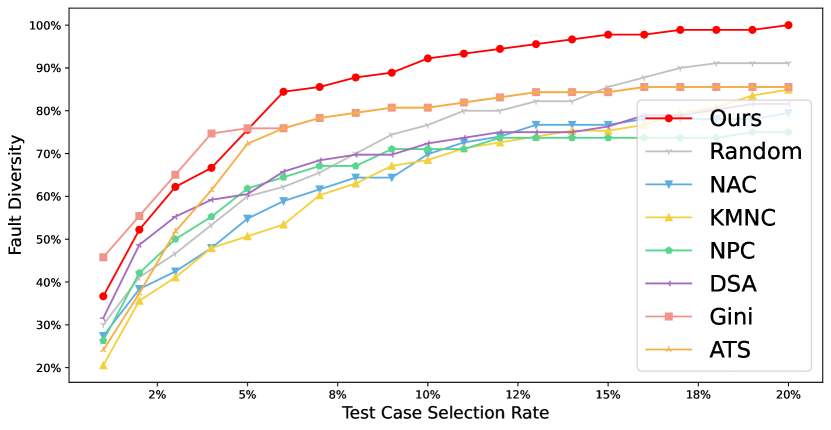
(c) CIFAR10 & ResNet20

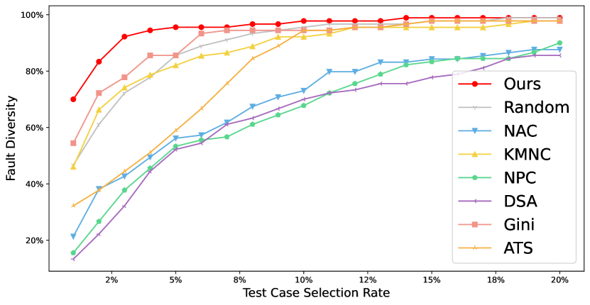
(d) SVHN & LeNet5

Figure 5: The cumulative sum of the fault types coverage rate (FTCR) found by our selection method. We only report four combinations due to page limitaion. Please refer to Tab. VIII for quantitative results.

IV-B3 Fault Type Detection Effectiveness

In this part, we delve deeper into the reasons why DeepFeature has a higher FDR and can increase more in accuracy than the baselines. Insights from traditional software testing found error-inducing inputs are very dense, inspiring DNN testing that detecting a greater variety of errors may also be as important as detecting more errors. We use the concept of fault type to answer this question. For a given test case $x$ that has been misclassified, its fault type is defined as:

$$Fault\_Type(x)=(Predict(x)\rightarrow Label(x))$$

where $Label(x)$ denotes the ground-truth label, and $Predict(x)$ denotes the DNN prediction. For instance, if the $Predict(x)$ is “7”, while the $Label(x)$ is “9”, then the fault type of $x$ is denoted as: $Fault\_Type(x)=7\rightarrow 9$. For a typical classification dataset with 10 different categories, the number of possible fault types is $10\times 9=90$. As the candidate test cases to be selected may not introduce all types of errors, we use the Fault Type Coverage Rate (FTCR), the proportion of error types introduced by our selected test cases among the error types introduced by all samples, to quantify the ability to select diverse faults.

Plots of FTCR with the percentage of selected cases increasing from 1% to 20% are shown in Fig. 5. Our selection method achieved better fault diversity compared to random selection and baseline methods under the vast majority of dataset&model combinations, indicating that DeepFeature can detect more types of faults in DNN, which explains why DeepFeature has higher FDR and can increase more accuracy compared with baselines. Second, we can see that in most of our experiments, the neuron coverage-driven selection stops increasing after the FTCR reaches 80%. Even if we increase the selection rate after that, their FTCR still converges to 80%. However, DeepFeature’s FTCR continues to increase to 100%, implying that some cases are not detected by neuron coverage-guided selection. In contrast, DeepFeature can detect them, implying that these cases will induce feature map types of errors.

As shown in the Tab. VIII, we also calculated the ratio of area under the curve (RAUC) of FTCR to quantitatively demonstrate how well each approach can identify various defects. It can be seen that existing neuron-coverage metrics are generally weaker than even random selection in terms of detecting diverse defects. Homogeneous faults from neuron coverage guided selection make only a trivial contribution to follow-up repairing. Nevertheless, DeepFeature tries to select more types of faults, yielding greater accuracy improvement after retraining (repairing) the model.

IV-C RQ2: How effective and efficient is DeepFeature’s fuzzing algorithm?

To answer this question, we compare DeepFeature with the SOTA fuzzing algorithm ADAPT and DeepMutation++ (DeepM++), and DeepHyperion (DeepH). We run DeepFeature and baselines for the same period of time (i.e., 5 minutes) to generate test cases. For the baselines’ parameter, we follow the default settings in its original paper (i.e., the fuzzing time for each case is limited to 1 second, and the coverage follows Tab. V). Then we retrain the models with generated cases and re-evaluate them to compare the accuracy improvement brought by DeepFeature and baselines.

Table IX shows our experiment results. We can see that for the same amount of time, DeepFeature can mutate more valuable fuzzing cases, which will be misclassified by the model, than baselines. Then, we also evaluate the quality of the fuzzing cases generated by baselines and ours. Considering baselines’ fuzzing cases are less than DeepFeature, we randomly select the same number of cases from DeepFeature to make a fair comparison for the fuzzing effectiveness (e.g., we only select 771 cases from DeepFeature in MNIST & LeNet1 combination). We then retrain the model using these fuzzing cases. Experiment results reveal that DeepFeature brings greater improvement on model accuracy in the majority of dataset & model combinations (e.g., we improve the accuracy of MNIST&LeNet1 into 93.45%, while baselines only improve to 92.84% and 92.88%.), denoting that test cases fuzzed by DeepFeature are more valuable than baselines.

Then, we can also observe that compared with DeepH, DeepFeature can generate more misclassified cases 5 to 20 times, which is because DeepHyperion will use illumination search to generate test cases for each feature map in the model, which causes it becomes time-consuming. Then we can also observe that using the same number of cases to repair the model, DeepFeature can increase more accuracy compared with DeepH, which is because cases generated by DeepFeature are focused on repairing vulnerable feature maps, while cases generated by DeepH may fine-tune the feature maps that are robustness, which decrease the repairing efficiency.

IV-D Can DeepFeature behave stable under different settings?

The FDR experiment results in Tab. VI are based on the five most vulnerable feature maps across all datasets and models. However, a fixed number of feature maps may not generalize well to models of different sizes, so we also analyze how the number of vulnerable feature maps would affect the estimation of the value of a test case and further affect the FDR. Specifically, for each experiment combination, we use the top-1, 5, 10, 15, 20, and 25 vulnerable feature maps to guide test case selection. Results are listed in Tab. X. We find that once the number of selected vulnerable feature maps are larger than 5, the effectiveness of DeepFeature will become stable. For instance, when number from 5 to 25, DeepFeature’s FDR only change from 62.10% to 62.01% in MNIST&LeNet1 combination, and the RAUC only change from 87.97% to 88.55%, which indicate the DeepFeature are stable under different number of selected vulnerable feature maps.

Perturbation.

In Algorithm 1, we will use $\epsilon$ to constrain the maximum perturbation of the FMA. To evaluate the impact of $\epsilon$ and $\alpha$ for the model, use four different $\epsilon$ and $\alpha$ setting to compare DeepFeature’s effectivenss (for ease of discussion, we set $\alpha=\epsilon/4$). The experiment results are shown in Tab. XI. We can observe that under different perturbation strength, DeepFeature’s effectiveness do not have large change for each model. For instance, when $\alpha$ increase from $1/255$ to $4/255$, DeepFeature’s FDR only change from 62.10% to 62.29% in MNIST&LeNet1 combination, and the RAUC also only change from 87.97% to 88.17%, which indicate DeepFeature are stable under different perturbation size.

Dataset	MNIST		Fashion		CIFAR10		SVHN
Model	LeNet1	LeNet5	LeNet1	ResNet20	VGG16	ResNet20	LeNet5	VGG16
NAC	57.36	55.49	54.12	46.71	58.81	65.53	69.75	47.15
KMNC	81.48	55.86	81.57	52.63	65.39	64.71	88.35	47.98
NPC	50.68	61.29	52.78	63.15	62.07	65.07	65.61	49.84
DSA	59.77	56.46	60.72	70.45	77.03	68.27	63.83	67.02
Gini	85.00	85.33	82.96	62.28	62.23	78.53	91.54	88.47
ATS	84.48	83.98	81.57	62.28	63.48	75.42	80.96	85.69
RS	74.01	65.37	70.04	71.59	74.15	72.66	90.02	74.62
Our	87.97	86.03	84.86	70.07	77.25	79.42	95.17	86.11

TABLE VIII: When selecting 20% test cases, the ratio of area under the curve (RAUC) of FTCR plots.

	ADAPT	DeepM++	DeepH	Our
Dataset&Model	Cases/Acc(%)	Cases/Acc(%)	Cases/Acc(%)	Cases/Acc(%)
MNIST (LeNet1)	771/92.84	3071/92.88	2315/92.81	41196/93.45
MNIST (LeNet5)	2254/95.22	5032/96.31	2431/95.33	46048/97.92
Fashion (LeNet1)	6578/80.01	10571/82.77	7759/81.03	48202/85.36
Fashion (ResNet20)	1105/91.61	3086/91.83	1037/90.07	12422/91.75
SVHN (LeNet5)	11273/86.50	17533/86.37	13375/96.77	37724/87.59
SVHN (VGG16)	559/93.77	3989/93.20	1277/93.39	19411/94.21
CIFAR10 (VGG16)	732/83.61	2554/84.33	1132/83.55	10244/86.96
CIFAR10 (ResNet20)	1622/86.14	3488/86.93	2441/86.76	12255/88.86

TABLE IX: DeepFeature and baselines generated fuzz test cases, which will be misclassied by DNN, within 5 minutes. In the repairing experiments, we randomly select the same number of cases as ADAPT to eliminate the effect of training case size (e.g., we only select 771 cases from DeepFeature and other baseliens in MNIST & LeNet1). DeepM++ and DeepH mean DeepMutation++ and DeepHyerion.

Dataset (DNN)	FDR of Top k vulnerable feature maps
	1	5	10	15	20	25
MNIST (LeNet-1)	56.15	62.10	62.72	62.30	62.10	62.01
Fashion (ResNet-20)	46.85	60.70	60.30	60.01	58.30	58.30
SVHN (LeNet-5)	50.20	62.34	62.32	62.30	62.17	62.15
CIFAR-10 (ResNet-20)	51.30	50.40	50.15	49.80	50.35	50.75
Dataset (DNN)	RAUC of Top k vulnerable feature maps
	1	5	10	15	20	25
MNIST (LeNet-1)	88.09	87.97	88.31	88.42	88.51	88.55
Fashion (ResNet-20)	59.68	70.07	66.66	66.03	64.84	62.30
SVHN (LeNet-5)	84.78	95.17	94.82	95.23	94.46	95.10
CIFAR-10 (ResNet-20)	76.89	78.78	81.11	78.89	81.63	85.93

TABLE X: FDR and FTCR with the different number of vulnerable feature maps ranging from 5 to 25, when 20% of the test cases have been selected. We only report four combinations, while other combinations have similar results.

Dataset (DNN)	FDR of different $\alpha$
	1/255	2/255	3/255	/4/255
MNIST (LeNet-1)	62.10	62.17	62.24	62.29
Fashion (ResNet-20)	60.70	60.78	60.85	60.90
SVHN (LeNet-5)	62.34	62.39	62.43	62.48
CIFAR-10 (ResNet-20)	50.40	50.48	50.55	50.60
Dataset (DNN)	RAUC of different $\alpha$
	1/255	2/255	3/255	/4/255
MNIST (LeNet-1)	87.97	88.09	88.14	88.17
Fashion (ResNet-20)	70.07	70.14	70.17	70.18
SVHN (LeNet-5)	95.17	95.30	95.41	94.44
CIFAR-10 (ResNet-20)	78.78	78.89	78.89	78.90

TABLE XI: FDR and FTCR with the different $\alpha$ and $\epsilon$.

IV-E Threats to Validity

Test subject selection. The selection of evaluation subjects (i.e., datasets and DNN models) could be a threat to validity. We try to counter this by using four commonly studied datasets (i.e., MNIST, Fashion, SVHN, and CIFAR10); for DNN models, we use four well-known pre-trained DNN-based models (i.e., LeNet-1, LeNet-5, ResNet-20, and VGG-16) of different sizes and complexity ranging from 3,350 neurons up to more than 35,749,834 neurons. However, it doesn’t guarantee that DeepFeature can be applied to all models. Additional models will be used to evaluate DeepFeature in future work.

Data simulation. Another threat to validity comes from the augmented test input generation. In order to generate test cases, we choose seven well-used benign mutations (i.e., shift, rotation, scale, shear, contrast, brightness, and blur) as our baselines to simulate faults from different sources and granularity. Although these data simulations are very similar to virtual environment noise, it is impossible to guarantee that the distribution of the real unseen input is the same as our simulation. Additional experiments based on real unseen inputs need to be conducted in future work.

Parameters settings. The last threat could be the parameter settings in baselines. To compare with neuron coverage-guided and prioritization test set selection methods, we reproduced existing coverage methods for DNN, which may include user-defined parameters. By fine-tuning the parameter settings, the selected data could be different. To alleviate the potential bias, we follow the authors’ suggested settings or employ the default settings of the original papers. Due to page constrain, the impact of different $step\_size$ are not discussed in the paper, which will be evaluated in the future.

V Related Work

This section discusses the related work in two groups: testing the DNN model and deep learning testing.

V-A Neuron Coverage Metrics

Pei et al. [3] proposes the first white-box coverage criteria (i.e., NAC), which calculates the percentage of activated neurons. Since NAC is coase-grain neuron metric, DeepGauge [4] then extends NAC and proposes a set of more fine-grained coverage criteria by considering the distribution of neuron outputs from the training data. Noticing that DNNs have millions of neuron, testing all neuron is a large overhead,  [6] propose IDC, which focus on an important neuron in DNNs. Inspired by the coverage criteria in traditional software testing, some conventional coverage metrics [41, 42, 7] are proposed. DeepCover [41] proposes the MC/DC coverage of DNNs based on the dependence between neurons in adjacent layers. To explore how inputs affect neuron internal decision logic flow, Xie et al. [32] propose NPC to explore the neuron path coverage. DeepCT [42] adopts the combinatorial testing idea and proposes a coverage metric that considers the combination of different neurons at each layer. DeepMutation [7] adopts the mutation testing into DL testing and proposes a set of operators to generate mutants of the DNN. Furthermore, DeepConcolic [5] analyzed the limitation of existing coverage criteria and proposed a more fine-grained coverage metric that considers the relationships between two adjacent layers and the combinations of values of neurons at each layer. Since neuron coverage testing can not detect fault-inducing feature maps in the DNN, in this work, we propose DeepFeature to address this problem, which can detect faults that are induced by the feature maps in the DNN (Sec. IV-B).

V-B Deep Learning Testing

Pei et al. [3] propose the first deep learning testing technique (i.e., DeepXplore), which test DNN internal neuron activation parttern. Based on the DeepXplore’s coverage metric, Tian et al. [26] propose DeepTest, which is used to generate test cases to explore DNN behaviors. Noticing DeepXplore is coarse-grained, Ma et al. [4] propose DeepGuage, which tests DNN by fine-grained metrics. Based on the DeepGauge [4], Ma et al. [7] propose DeepMutation [7] and DeepMutation++ [15], these techniques are used to mutate test case to explore model incorrect behaviors.  Odena et al. [29] also uses metrics proposed by the above-mentioned coverage metric to generate test cases. Since the test cases generated are not always useful, and feeding all test cases into the model is time-consuming and the benign selection strategies used by coverage metrics are also time-consuming,

Based on the above-mentioned testing techniques, some automated testing techniques [41, 29, 3, 26, 5, 15, 12] are proposed to generate test inputs towards explore DNN incorrect behaviours. In addition, while the neuron coverage guided testing techniques are widely studied, the existing work [10, 25, 28, 27] found that using NC-guided testing can not detect all types of faults in DNN. Such findings motivate this work that proposes a new type of test unit, i.e., feature map, to detect more types of faults that are not detected by neuron criteria testing techniques.

VI Conclusion

In this work, we propose DeepFeature, which test DNNs from feature map level, for testing DNNs. Unlike existing neuron testing techniques, DeepFeature take the feature map as a testing unit, which delves into every inner feature maps that the models learned and detects vulnerable ones in the testing process. The key component of DeepFeature is its testing metrics called FVS and FAS. FVS quantifies the vulnerability of the model feature maps, and FAS measures the impact of vulnerable feature maps on the model’s accuracy. Then we propose a new feature map guided test case selection, which selects test cases by measuring each test case’s FVS value in vulnerable feature maps. Compared with coverage-guided and prioritization test case selection methods, DeepFeature’s test case selection increases the fault detection rate by 49.97% and 24.8% on average, respectively. Finally, we utilize the proposed FVS metric to automatically fuzz for more valuable test cases to repair vulnerable feature maps and improve the model’s accuracy. The source code of DeepFeature with all the evaluation details are available on our Github Page [43].

References

- Bojarski et al. [2016] M. Bojarski, D. W. del Testa, D. Dworakowski, B. Firner, B. Flepp, P. Goyal, L. D. Jackel, M. Monfort, U. Muller, J. Zhang, X. Zhang, J. Zhao, and K. Zieba, “End to end learning for self-driving cars,” ArXiv, vol. abs/1604.07316, 2016.
- Rajpurkar et al. [2017] P. Rajpurkar, J. A. Irvin, K. Zhu, B. Yang, H. Mehta, T. Duan, D. Y. Ding, A. Bagul, C. Langlotz, K. S. Shpanskaya, M. P. Lungren, and A. Ng, “Chexnet: Radiologist-level pneumonia detection on chest x-rays with deep learning,” ArXiv, vol. abs/1711.05225, 2017.
- Pei et al. [2017] K. Pei, Y. Cao, J. Yang, and S. Jana, “Deepxplore: Automated whitebox testing of deep learning systems,” in proceedings of the 26th Symposium on Operating Systems Principles, 2017, pp. 1–18.
- Ma et al. [2018a] L. Ma, F. Juefei-Xu, F. Zhang, J. Sun, M. Xue, B. Li, C. Chen, T. Su, L. Li, Y. Liu et al., “Deepgauge: Multi-granularity testing criteria for deep learning systems,” in Proceedings of the 33rd ACM/IEEE International Conference on Automated Software Engineering, 2018, pp. 120–131.
- Sun et al. [2018a] Y. Sun, M. Wu, W. Ruan, X. Huang, M. Kwiatkowska, and D. Kroening, “Concolic testing for deep neural networks,” 2018 33rd IEEE/ACM International Conference on Automated Software Engineering (ASE), pp. 109–119, 2018.
- Gerasimou et al. [2020] S. Gerasimou, H. F. Eniser, A. Sen, and A. Cakan, “Importance-driven deep learning system testing,” 2020 IEEE/ACM 42nd International Conference on Software Engineering: Companion Proceedings (ICSE-Companion), pp. 322–323, 2020.
- Ma et al. [2018b] L. Ma, F. Zhang, J. Sun, M. Xue, B. Li, F. Juefei-Xu, C. Xie, L. Li, Y. Liu, J. Zhao, and Y. Wang, “Deepmutation: Mutation testing of deep learning systems,” 2018 IEEE 29th International Symposium on Software Reliability Engineering (ISSRE), pp. 100–111, 2018.
- Jahangir and Shafait [2022] M. Jahangir and F. Shafait, “Adversarial attack using sparse representation of feature maps,” IEEE Access, vol. 10, pp. 120 724–120 734, 2022.
- Wang et al. [2021a] Z. Wang, H. Guo, Z. Zhang, W. Liu, Z. Qin, and K. Ren, “Feature importance-aware transferable adversarial attacks,” in Proceedings of the IEEE/CVF international conference on computer vision, 2021, pp. 7639–7648.
- Harel-Canada et al. [2020] F. Harel-Canada, L. Wang, M. A. Gulzar, Q. Gu, and M. Kim, “Is neuron coverage a meaningful measure for testing deep neural networks?” ser. ESEC/FSE 2020. New York, NY, USA: Association for Computing Machinery, 2020, p. 851–862. [Online]. Available: https://doi.org/10.1145/3368089.3409754
- Li et al. [2019a] Z. Li, X. Ma, C. Xu, and C. Cao, “Structural coverage criteria for neural networks could be misleading,” in 2019 IEEE/ACM 41st International Conference on Software Engineering: New Ideas and Emerging Results (ICSE-NIER), 2019, pp. 89–92.
- Xie et al. [2018] X. Xie, L. Ma, F. Juefei-Xu, H. Chen, M. Xue, B. Li, Y. Liu, J. Zhao, J. Yin, and S. See, “Deephunter: Hunting deep neural network defects via coverage-guided fuzzing,” arXiv: Software Engineering, 2018.
- Lee et al. [2020] S. Lee, S. Cha, D. Lee, and H. Oh, “Effective white-box testing of deep neural networks with adaptive neuron-selection strategy,” in Proceedings of the 29th ACM SIGSOFT International Symposium on Software Testing and Analysis, ser. ISSTA 2020. New York, NY, USA: Association for Computing Machinery, 2020, p. 165–176. [Online]. Available: https://doi.org/10.1145/3395363.3397346
- Kim et al. [2019] J. Kim, R. Feldt, and S. Yoo, “Guiding deep learning system testing using surprise adequacy,” in 2019 IEEE/ACM 41st International Conference on Software Engineering (ICSE). IEEE, 2019, pp. 1039–1049.
- Hu et al. [2019] Q. Hu, L. Ma, X. Xie, B. Yu, Y. Liu, and J. Zhao, “Deepmutation++: A mutation testing framework for deep learning systems,” in 2019 34th IEEE/ACM International Conference on Automated Software Engineering (ASE), 2019, pp. 1158–1161.
- Deng [2012] L. Deng, “The mnist database of handwritten digit images for machine learning research,” IEEE Signal Processing Magazine, vol. 29, no. 6, pp. 141–142, 2012.
- LeCun et al. [1998] Y. LeCun, L. Bottou, Y. Bengio, and P. Haffner, “Gradient-based learning applied to document recognition,” Proceedings of the IEEE, vol. 86, no. 11, pp. 2278–2324, 1998.
- Krizhevsky [2009] A. Krizhevsky, “Learning multiple layers of features from tiny images,” Tech. Rep., 2009.
- He et al. [2016] K. He, X. Zhang, S. Ren, and J. Sun, “Deep residual learning for image recognition,” in Proceedings of the IEEE conference on computer vision and pattern recognition, 2016, pp. 770–778.
- Simonyan and Zisserman [2014] K. Simonyan and A. Zisserman, “Very deep convolutional networks for large-scale image recognition,” arXiv preprint arXiv:1409.1556, 2014.
- Xiao et al. [2017] H. Xiao, K. Rasul, and R. Vollgraf. (2017) Fashion-mnist: a novel image dataset for benchmarking machine learning algorithms.
- Netzer et al. [2011a] Y. Netzer, T. Wang, A. Coates, A. Bissacco, B. Wu, and A. Y. Ng, “Reading digits in natural images with unsupervised feature learning,” 2011.
- Wang et al. [2021b] J. Wang, J. Chen, Y. Sun, X. Ma, D. Wang, J. Sun, and P. Cheng, “Robot: Robustness-oriented testing for deep learning systems,” 2021 IEEE/ACM 43rd International Conference on Software Engineering (ICSE), pp. 300–311, 2021.
- Netzer et al. [2011b] Y. Netzer, T. Wang, A. Coates, A. Bissacco, B. Wu, and A. Ng, “Reading digits in natural images with unsupervised feature learning,” 2011.
- Feng et al. [2020] Y. Feng, Q. Shi, X. Gao, J. Wan, C. Fang, and Z. Chen, “Deepgini: Prioritizing massive tests to enhance the robustness of deep neural networks,” in Proceedings of the 29th ACM SIGSOFT International Symposium on Software Testing and Analysis, ser. ISSTA 2020. New York, NY, USA: Association for Computing Machinery, 2020, p. 177–188. [Online]. Available: https://doi.org/10.1145/3395363.3397357
- Tian et al. [2018] Y. Tian, K. Pei, S. S. Jana, and B. Ray, “Deeptest: Automated testing of deep-neural-network-driven autonomous cars,” 2018 IEEE/ACM 40th International Conference on Software Engineering (ICSE), pp. 303–314, 2018.
- Gao et al. [2022] X. Gao, Y. Feng, Y. Yin, Z. Liu, Z. Chen, and B. Xu, “Adaptive test selection for deep neural networks,” in 2022 IEEE/ACM 44th International Conference on Software Engineering (ICSE), 2022, pp. 73–85.
- Li et al. [2019b] Z. Li, X. Ma, C. Xu, and C. Cao, “Structural coverage criteria for neural networks could be misleading,” in 2019 IEEE/ACM 41st International Conference on Software Engineering: New Ideas and Emerging Results (ICSE-NIER). IEEE, 2019, pp. 89–92.
- Odena et al. [2019] A. Odena, C. Olsson, D. Andersen, and I. Goodfellow, “TensorFuzz: Debugging neural networks with coverage-guided fuzzing,” in Proceedings of the 36th International Conference on Machine Learning, ser. Proceedings of Machine Learning Research, K. Chaudhuri and R. Salakhutdinov, Eds., vol. 97. PMLR, 09–15 Jun 2019, pp. 4901–4911. [Online]. Available: https://proceedings.mlr.press/v97/odena19a.html
- Guo et al. [2018] J. Guo, Y. Jiang, Y. Zhao, Q. Chen, and J. Sun, “Dlfuzz: differential fuzzing testing of deep learning systems,” Proceedings of the 2018 26th ACM Joint Meeting on European Software Engineering Conference and Symposium on the Foundations of Software Engineering, 2018.
- Zohdinasab et al. [2021] T. Zohdinasab, V. Riccio, A. Gambi, and P. Tonella, “Deephyperion: Exploring the feature space of deeplearning-based systems through illumination search,” in Proceedings of the ACM SIGSOFT International Symposium on Software Testing and Analysis, ser. ISSTA ’21. Association for Computing Machinery, 2021.
- Xie et al. [2022] X. Xie, T. Li, J. Wang, L. Ma, Q. Guo, F. Juefei-Xu, and Y. Liu, “Npc: Neuron path coverage via characterizing decision logic of deep neural networks,” ACM Transactions on Software Engineering and Methodology (TOSEM), vol. 31, pp. 1 – 27, 2022.
- Wang et al. [2021c] Z. Wang, H. You, J. Chen, Y. Zhang, X. Dong, and W. Zhang, “Prioritizing test inputs for deep neural networks via mutation analysis,” 2021 IEEE/ACM 43rd International Conference on Software Engineering (ICSE), pp. 397–409, 2021.
- Ren et al. [2020] P. Ren, Y. Xiao, X. Chang, P.-Y. Huang, Z. Li, X. Chen, and X. Wang, “A survey of deep active learning,” ACM Computing Surveys (CSUR), vol. 54, pp. 1 – 40, 2020.
- Madry et al. [2017] A. Madry, A. Makelov, L. Schmidt, D. Tsipras, and A. Vladu, “Towards deep learning models resistant to adversarial attacks,” arXiv preprint arXiv:1706.06083, 2017.
- Chen et al. [2020] J. Chen, Z. Wu, Z. Wang, H. You, L. Zhang, and M. Yan, “Practical accuracy estimation for efficient deep neural network testing,” ACM Transactions on Software Engineering and Methodology (TOSEM), vol. 29, pp. 1 – 35, 2020.
- Zhang et al. [2019] H. Zhang, Y. Yu, J. Jiao, E. P. Xing, L. E. Ghaoui, and M. I. Jordan, “Theoretically principled trade-off between robustness and accuracy,” ArXiv, vol. abs/1901.08573, 2019.
- Gligorić et al. [2015] M. Gligorić, L. Eloussi, and D. Marinov, “Practical regression test selection with dynamic file dependencies,” Proceedings of the 2015 International Symposium on Software Testing and Analysis, 2015.
- Zhang [2018] L. Zhang, “Hybrid regression test selection,” 2018 IEEE/ACM 40th International Conference on Software Engineering (ICSE), pp. 199–209, 2018.
- Legunsen et al. [2016] O. Legunsen, F. Hariri, A. Shi, Y. Lu, L. Zhang, and D. Marinov, “An extensive study of static regression test selection in modern software evolution,” Proceedings of the 2016 24th ACM SIGSOFT International Symposium on Foundations of Software Engineering, 2016.
- Sun et al. [2018b] Y. Sun, X. Huang, and D. Kroening, “Testing deep neural networks,” ArXiv, vol. abs/1803.04792, 2018.
- Ma et al. [2019] L. Ma, F. Juefei-Xu, M. Xue, B. Li, L. Li, Y. Liu, and J. Zhao, “Deepct: Tomographic combinatorial testing for deep learning systems,” 2019 IEEE 26th International Conference on Software Analysis, Evolution and Reengineering (SANER), pp. 614–618, 2019.
- DeepFeature [2022] DeepFeature, “Deepfeature,” 2022. [Online]. Available: https://github.com/ASE2023Paper/deepfeature/