Symmetry Analysis with Spin Crystallographic Groups:
Disentangling Spin-Orbit-Free Effects
in Emergent Electromagnetism

Abstract

Recent studies identified spin-order-driven phenomena such as spin-charge interconversion without relying on the relativistic spin-orbit interaction. Those physical properties can be prominent in systems containing light magnetic atoms due to sizable exchange splitting and may pave the way for realizations of giant responses correlated with the spin degree of freedom. In this paper, we present a systematic symmetry analysis based on the spin crystallographic groups and identify physical property of an vast number of magnetic materials up to 1500 in total. Absence of spin-orbital entanglement leads to the spin crystallographic symmetry having richer property compared to the well-known magnetic space group symmetry. By decoupling the spin and orbital degrees of freedom, our analysis enables us to take a closer look into the relation between the dimensionality of spin structures and the resultant physical properties and to identify the spin and orbital contributions separately. In stark contrast to the established analysis with magnetic space groups, the spin crystallographic group manifests richer symmetry including spin translation symmetry and leads to nontrivial emergent responses. For representative examples, we discuss geometrical nature of the anomalous Hall effect and magnetoelectric effect, and classify the spin Hall effect arising from the spontaneous spin-charge coupling. Using the power of computational analysis, we apply our symmetry analysis to a wide range of magnets, encompassing complex magnets such as those with noncoplanar spin structures as well as collinear and coplanar magnets. We identify emergent multipoles relevant to physical responses and argue that our method provides a systematic tool for exploring sizable electromagnetic responses driven by spin ordering.

I introduction

Spintronics has experienced tremendous growth, and the concept has been discussed in various fields including topological electronic systems and superconductors. In recent years, spin-orbit coupling (SOC), a relativistic interaction between the charge and spin degrees of freedom, is particularly of matter due to its rich physical consequences. Search for candidate materials have been taken place to maximize the physical responses associated with spin-orbit interaction in these decades. For example, giant spin-momentum splittings have been identified in systems with heavy atoms having large SOC. Their strong spin-orbital entanglement has been demonstrated by spectroscopy [1, 2] and transport measurements [3]. The progress may let us consider the possibility of physics originating from SOC covering a broader range of materials other than what consists of heavy atoms, such as materials based on $3d$ transition metal elements with negligible relativistic SOC.

To this end, a concept of spontaneous spin-charge locking has been proposed in theories [4, 5, 6, 7]. This coupling arises from the spontaneous magnetic ordering, which can exhibit exchange splitting energy comparable to the Coulomb interaction. The concept illuminates the potential impacts of light elements for the spintronic application and further identified advantageous properties compared to conventionally-studied materials; e.g., strong exchange splitting energy and large transition temperature. Notably, the magnetic order gives rise to characteristic spin-momentum-locking structure due to coupling between the order and structural property of crystals as found in antiferromagnetic materials. These aspects are valuable for applications in the field of antiferromagnetic spintronics gathering considerable interest as an emerging field in condensed matter physics [8, 9, 10]; for instance, various physical phenomena free from SOC have been clarified in the previous works such as the spin-polarized current induction [11, 12, 13, 14, 15], nonlinear response [16, 17], piezomagnetic effect [4, 18], and magnetoresistance [19].

Released from the SOC constraint, the array of localized spins does not have any favorable orientation described by the crystal structure. The decoupling between spin and orbital degrees of freedom leads to a magnetic symmetry higher than the conventional magnetic space group symmetry (Shubnikov group). Such magnetic symmetry without SOC is covered by the spin crystallographic group [20, 21] which includes a richer group structure due to the absence of SOC. The spin crystallographic groups have applied to analyzing the electronic structure modified by the spontaneous spin order, particularly in the case of the order labeled by the zero propagation vector such as collinear antiferromagnetic order [4, 5, 22, 7].

In spite of intensive studies of those having collinear spin structures dubbed as altermagnets [10], non-zero propagation spin structures have not been fully investigated from the viewpoint of spin-crystallographic-group symmetry. This class of magnetic materials encompasses intriguing systems such as noncoplanar magnets and multiferroic magnets. A prototypical phenomena unique to these materials is the geometrical Hall effect [23]. The effect stems from the fictitious magnetic flux formed by the noncoplanar spin structure observed in materials such as systems with a triangular or kagomé net. The resultant time-reversal-symmetry breaking mimics the orbital-flux order proposed in Ref. [24], and does not require the relativistic SOC effect. The SOC-free nature is in highly-contrast to the well-known anomalous Hall effect arising from the collinear and coplanar spin order [25, 26, 27] and may be responsible for the anomalous Hall responses of magnetic skyrmion crystals [28, 29]. These prior studies indicate that the dimension of the spin structure is key to identifying the emergent physical responses induced by the spin order without the help of SOC. In this regard, the spin crystallographic group is advantageous compared to the widely-used magnetic space group, because its group symmetry reflects a given spin-structure dimension.

In this paper, we present the spin-group symmetry analysis covering not only the simple magnetic materials having collinear and coplanar spin structures but also complex spin-ordered systems such as noncoplanar magnets and those with non-zero propagation vectors. The analysis incorporates the dimensionality of the spin structure and hence provides a convenient tool for identifying the emergent symmetry breaking and associated phenomena which cannot been distinguished from the SOC-assisted contribution in terms of the SOC-accounted symmetry analysis (magnetic space/point group analysis) [30].

Specifically, we demonstrate the following points of the present symmetry analysis; by separating the spin and orbital spaces, we can identify the contribution of each degree of freedom to physical responses. Our method captures the non-trivial translation symmetry accompanied by the spin-space operation keeping high symmetry in the spin space, which is unexpected by the magnetic-space group analysis. The symmetry unique to the system without SOC implies the spin-geometry-induced response with negligible contribution due to the relativistic SOC effect. Furthermore, our result suggests that emergent physical responses can be examined in a semi-quantitative manner by combining the spin-group symmetry analysis with the physical insights into spin fluctuations correlated with the dimensionality of a spin structure. We explain these features by taking several physical properties such as the anomalous Hall effect, magnetoelectric effect, and spin Hall effect.

The symmetry analysis is computationally performed with the use of the algorithm for searching the spin space group developed by Shinohara et al. [31]. By classifying a vast number of magnetic materials ($\sim$ 1500), we systematically clarify the SOC-free emergent properties of real magnetic materials.

The organization of the paper is the following. In Sec. II, we overview the spin space group and introduce the symmetry analysis with it. Based on the spin point group, the symmetry analysis applies to some of ferromagnetic and antiferromagnetic materials and their physical responses in Sec. III. Section IV is devoted to a high-throughput symmetry analysis of magnetic materials listed in magndata [32, 33]. In the light of emergent magnetic multipoles and rotators for spin-charge coupling, we investigate the SOC-free physical properties and demonstrate that our symmetry analysis clarifies the importance of the spin-structure dimension. We summarize the contents in Sec. V. The procedure of the symmetry analysis is sketched in Fig. 1.

The symmetry analysis with given spin space group $\mathcal{G}$ and magnetic space group $\mathbf{G}$ are automatically computed on the basis of spglib [34, 35] and spinspg [31]. Terms related to group theory can be found in Appendix A.

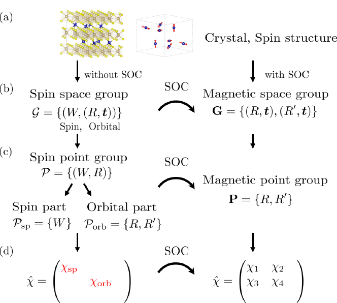
Figure 1: Procedure of symmetry analysis. (a) Input of crystal and spin structures. Dozens of data imported from magndata. (b) Spin space group $\mathcal{G}$ and magnetic space group $\mathbf{G}$ computationally identified. The effect of spin-orbit-coupling (SOC) is not considered in $\mathcal{G}$ but taken into account in $\mathbf{G}$. The spin-space-group symmetry is given by the spin rotation ($W$) and by orbital-space operations such as rotation ($R$) and translation ($\bm{t}$) operations. The magnetic space group comprises the orbital-space operations $(R,\bm{t})$ with or without the time-reversal operation $R^{\prime}=\theta R$. For the magnetic space group $\mathbf{G}$, the orbital-space operations $R,R^{\prime}$ also act on spins due to the SOC constraint. (c) The space group is reduced to its point group by omitting the translation operation $\bm{t}$. Spin ($\mathcal{P}$) and magnetic ($\mathbf{P}$) point groups are obtained from $\mathcal{G}$ and $\mathbf{G}$, respectively. The spin point group is further divided into ($\mathcal{P}_{\text{sp}},\mathcal{P}_{\text{orb}}$) consisting of either spin- or orbital-space symmetry. The spin crystallographic groups ($\mathcal{G},\mathcal{P}$) are reduced to the spin-orbital-coupled groups ($\mathbf{G},\mathbf{P}$) by SOC. (d) The symmetry-adapted form of a given tensor $\hat{\chi}$ obtained by the spin or magnetic point group symmetry. The red-colored components ($\chi_{\text{sp}},\chi_{\text{orb}}$) originates from the spin-ordering symmetry breaking without SOC, and the origin of each components is further distinguished into the spin ($\chi_{\text{sp}}$) and orbital ($\chi_{\text{orb}}$) degree of freedom. SOC entangles the spin contribution with the orbital ($\chi_{1},\chi_{4}$) and induces additional components ($\chi_{2},\chi_{3}$).

II Spin-group operations and spin crystallographic group

We introduce the transformation property of symmetry operations and overview the spin crystallographic symmetry such as the spin space group and spin point group. We do not detail the mathematical aspects of the spin crystallographic group. Interested readers can refer to Refs. [21, 36, 31].

Owing to the absence of generic spin-orbital coupling, the rotation operation separately acts on the spin and orbital space in terms of the spin group symmetry. Let $g=\left(R,W\right)$ be the combination of symmetry operations $W$ and $R$ acting on the spin and orbital space, respectively.

Firstly, we consider the point group symmetry with rotation operations $W,R$ and raise some examples of the basic transformation property such as position $\bm{r}$, momentum $\bm{p}$, and spin $\bm{s}$. For instance, let us take the orbital-space-only operation $g_{\text{orb}}=\left(R,1\right)$, the time-reversal operation $\theta=\left(1,-1\right)$, and spin-space proper rotation $g_{\text{sp}}=\left(1,W\right)$ (det $W=+1$). The operators are transformed under each symmetry operation as shown in Fig. 2. The anti-unitary property of a given symmetry operation is represented by the improperness of the spin-space operation $W$; i.e., $g=\left(R,W\right)$ is unitary for $\text{det}\,W=+1$ and anti-unitary for $\text{det}\,W=-1$. Thus, the time-reversal operation $\theta$ can act on the orbital space as it flips the time-reversal-odd quantities, e.g., $\bm{p}$ [Fig. 2(b)] and orbital magnetization. On the other hand, the proper rotation in the spin space does affect only the spin degree of freedom [Fig. 2(c)]. For a spin-group operation $g=\left(R,W\right)$, the operators are transformed as

$$g\,r_{a}\,g^{-1} =r_{b}T_{ba}(R),$$ (1)

$$g\,p_{a}\,g^{-1} =\text{det}W\cdot p_{b}T_{ba}(R),$$ (2)

$$g\,s_{a}\,g^{-1} =s_{b}T_{ba}(W),$$ (3)

where we introduced the three-dimensional orthogonal matrices $\hat{T}(u)$ ($u\in\text{O(3)}$) in accordance with the vectorial symmetry of each object.

We generalize the symmetry argument to the case of the tensor quantity $O_{abc\cdots}$. The transformation is written by

$$g\,O_{abc\cdots}\,g^{-1} =O_{a^{\prime}b^{\prime}c^{\prime}\cdots}D_{a^{\prime}a}^{(A)}(g)D_{b^{\prime}b}^{(B)}(g)D_{c^{\prime}c}^{(C)}(g)\cdots,$$ (4)

where we introduced the representation matrices for physical quantities $A,B,C,\cdots$ labeled by the indices $a,b,c,\cdots$, respectively. For the afore-mentioned three quantities, the representation matrices are explicitly given by

$$\hat{D}^{(r)}(g)=\hat{T}(R),~{}\hat{D}^{(p)}(g)=\text{det}\,W\cdot\hat{T}(R),~{}\hat{D}^{(s)}(g)=\hat{T}(W).$$ (5)

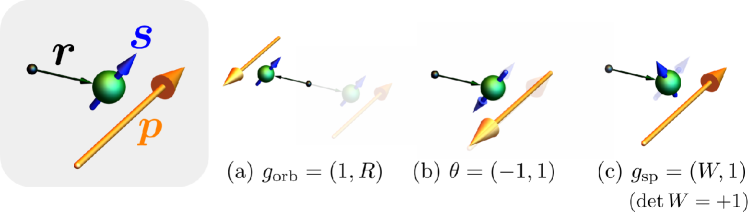
Figure 2: Spin-group transformation of electron depicted by position $\bm{r}$, momentum $\bm{p}$, and spin $\bm{s}$. The spin-group operation $g=\left(R,W\right)$ ($W$ is spin-space rotation, $R$ is orbital-space rotation). (a) Orbital-space operation ($W=1$) acting on position and momentum while leading to no action on spins. (b) Spin-space inversion operation same as the time-reversal operation ($W=-1,~{}R=1$). (c) Spin-space operation ($R=1$) satisfying the proper-rotation condition (det $W=+1$). It gives no transformation related with the orbital-space objects.

Next, we consider the structure of the group consisting of spin-group operations. In terms of the space group symmetry, the orbital-space operation $h$ is comprised of the point group operation $R$ and the translation operation $\bm{t}$ as $h=\left(R,\bm{t}\right)$. The spin space group $\mathcal{G}$ is a set of symmetry operations $g=\left(h,W\right)$ under which crystal structures and spin configuration dwelling on each magnetic atom are invariant. In stark contrast to the well-known magnetic space group (Shubnikov group) $\mathbf{G}$ [37], we can take symmetry operations acting on objects in the orbital and spin space independently [36]. The difference can be inferred from the adopted Hamiltonian.

Let us consider Hamiltonian having the spin-space-group symmetry. The Hamiltonian not only consists of kinetic and potential Hamiltonians $H_{0}$ for paramagnetic states but also takes into account the spontaneous spin ordering as the molecular field. The total Hamiltonian is given by

$$H_{\text{SG}}=H_{0}+H_{\text{mag}},$$ (6)

where the molecular-field term is

$$H_{\text{mag}}=\sum_{i}\bm{B}^{(i)}\cdot\bm{s}^{(i)},$$ (7)

with the indices for the sites $i$. The exchange-splitting field $\bm{B}^{(i)}$ is defined at each magnetic site ($\bm{B}^{(i)}=\bm{0}$ for nonmagnetic atoms). The Hamiltonian [Eq. (6)] is invariant under the associated spin space group as

$$g\in\mathcal{G},~{}g\,H_{\text{SG}}\,g^{-1}=H_{\text{SG}}.$$ (8)

The paramagnetic part satisfies the following relation for $g=\left(h,W\right)\in\mathcal{G}$ as

$$\left(h,W\right)H_{0}\left(h,W\right)^{-1}=\left(h,1\right)H_{0}\left(h,1\right)^{-1}=H_{0},$$ (9)

where the spin rotation $W$ is irrelevant. The orbital-space part $h$ is therefore restricted by the atomic configuration and generated by the space group of a given crystal structure. On the other hand, the exchange Hamiltonian is transformed by both of $h$ and $W$ as

$$g\left(\sum_{i}B_{a}^{(i)}s_{a}^{(i)}\right)g^{-1} =\sum_{i}B_{a}^{(i)}\cdot\left(g\,s_{a}^{(i)}\,g^{-1}\right),$$ (10)

$$=\sum_{i}B_{a}^{(i)}\cdot s_{b}^{(i_{h})}T_{ba}(W).$$ (11)

The orbital-space operation permutes the sites as $h:\bm{r}_{i}\mapsto\bm{r}_{i_{h}}=h^{-1}\,\bm{r}_{i}\,h$. Owing to Eq. (8), the spin-group operations should satisfy

$$\hat{T}(W)\,\bm{B}^{(i)}=\bm{B}^{(i_{h})},$$ (12)

for every site, and the coupling spontaneously arises between the orbital and spin degrees of freedom. Importantly, the operations $h$ and $W$ are taken in an independent manner as long as they satisfy Eq. (12). The property clearly distinguishes the spin space group from the magnetic space group.

For the case of the magnetic space group, we similarly treat the magnetic order as the molecular fields and further add spin-orbit interaction $H_{\text{SOC}}$ to the Hamiltonian. The Hamiltonian reads

$$H_{\text{MG}}=H_{0}+H_{\text{mag}}+H_{\text{SOC}},$$ (13)

where the SOC Hamiltonian is explicitly given by

$$H_{\text{SOC}} =\lambda\bm{L}\cdot\bm{s}.$$ (14)

$\bm{L}$ denotes the orbital angular momentum and $\lambda$ is the strength of SOC. The additional symmetry constraint by the SOC Hamiltonian leads to the the group-subgroup relation $\mathcal{G}$ ($\mathbf{G}<\mathcal{G}$). In stark contrast to the spin space group $\mathcal{G}$, the SOC Hamiltonian imposes the following constraint on $\left(h,W\right)=\left(\left(R,\bm{t}\right),W\right)\in\mathbf{G}$,

$$\text{det}R\cdot R=\text{det}W\cdot W.$$ (15)

That is, the proper-rotation parts in $h$ and $W$ should be the same as each other [31]. Eq. (15), along with Eq. (12), ties the orbital space with the spin space.

Then, let us overview the group structure of spin space group $\mathcal{G}$ which has been investigated in Refs. [38, 36, 31]. $\mathcal{G}$ comprises the spin-only group $\mathcal{G}_{\text{so}}$ as a normal subgroup ($\mathcal{G}\triangleright\mathcal{G}_{\text{so}}$). The spin-only group solely consists of the spin symmetry operations such as

$$\mathcal{G}_{\text{so}}=\left((1,\bm{0}),\mathcal{P}_{\text{so}}\right)=\{\left((1,\bm{0}),W\right)\}.$$ (16)

The group is determined by the dimension of a given spin configuration [21]. For one-dimensional magnets (collinear magnets), the magnetic moments are parallel or anti-parallel to the axis $\bm{n}$ in the spin space. The spin-only group is given by an internal semidirect product,

$$\mathcal{P}_{\text{so}}=\text{SO(2)}\rtimes\{1,m_{\parallel}\},$$ (17)

by which the vector $\bm{n}$ axis is invariant. we can take rotation operations along $\bm{n}$ with an arbitrary angle and mirror reflection $m_{\parallel}$ whose mirror plane contains the axis $\bm{n}$. For the two-dimensional (noncollinear but coplanar) case, the spin-only group is

$$\mathcal{P}_{\text{so}}=\{1,m_{\perp}\}.$$ (18)

The mirror operation $m_{\perp}$ shares its plane with the spins spanning the two-dimensional plane. Lastly, in the three-dimensional (noncoplanar) case, the spin-only group is trivial

$$\mathcal{P}_{\text{so}}=\{1\}.$$ (19)

By using the spin-only group, the spin space group is decomposed as [38]

$$\mathcal{G}=\mathcal{G}_{\text{so}}\times\overline{\mathcal{G}}.$$ (20)

As a result, we obtain the nontrivial spin space group $\overline{\mathcal{G}}$ whose spin-space operation $W$ is the identity or intimately coupled to the orbital-space operation $h=(R,\bm{t})$ such as the combined operation of spin rotation and translation $g=\left((1,\bm{t}),W\right)$; i.e., the symmetry operation $\left((R,\bm{t}),W\right)$ with $W\neq 1$ satisfies $(R,\bm{t})\neq(1,\bm{0})$. The set of spin translation operations $\{\left((1,\bm{t}),W\right)\}$ forms the group which we denote the spin translation group $\overline{\mathcal{G}}_{\text{st}}$. When the spin ordering does not modify the paramagnetic unit cell, the spin translation group is the translation group $\mathcal{T}=\{\left((1,\bm{t}),1\right)\}$ spanned by the Bravais vectors. The spin translation group is a normal subgroup of the nontrivial spin space group ($\overline{\mathcal{G}}\triangleright\overline{\mathcal{G}}_{\text{st}}$). Thus, we decompose $\overline{\mathcal{G}}$ by $\overline{\mathcal{G}}_{\text{st}}$ as

$$\overline{\mathcal{G}}=\bigcup_{i}~{}\overline{g}_{i}\,\overline{\mathcal{G}}_{\text{st}}.$$ (21)

The representative operation $\overline{g}_{i}=\left(\left(R,\bm{t}\right),W\right)$ indicates that the spin-space operation accompanies with the orbital-space operations but otherwise the identity ($W=1$); in other words, the orbital-space point group operation is nontrivial ($R\neq 1$) except for the identity operation $\left((1,\bm{0}),1\right)$. The complete tabulation of the spin space group $\mathcal{G}$ has not been accomplished while $\mathcal{G}$ of given crystal and spin structures can be computationally obtained [31].

For instance, we consider the body-centered-cubic Fe (space group $Im\bar{3}m$) whose ferromagnetic spin polarization is along the $[001]$ axis. The magnetic space group $\mathbf{G}=I4/mm^{\prime}m^{\prime}$ indicates the spontaneous crystalline symmetry reduction from the cubic to tetragonal under the SOC effect. On the other hand, the spin space group $\mathcal{G}$ retains high symmetry in the ordered state. The spin space group comprises the spin-only group $\mathcal{G}_{\text{so}}$ given by Eq. (17) with the spin-space axis $\bm{n}=[001]$. By dividing $\mathcal{G}$ by the spin-only group, we obtain the nontrivial spin space group $\overline{\mathcal{G}}$ [Eq. (20)]. Since the ferromagnetic order does not modify the unit cell, the spin translation group is trivially the translation group $\mathcal{T}_{\text{bcc}}$ for the bcc centering;

$$\overline{\mathcal{G}}=\bigcup_{i}~{}\overline{g}_{i}\,\overline{\mathcal{G}}_{\text{st}}=\bigcup_{i}~{}\overline{g}_{i}\mathcal{T}_{\text{bcc}},$$ (22)

where $\{\overline{g}_{i}\}$ forms the cubic point group same as that for the paramagnetic state ($m\bar{3}m$). As a result, the nontrivial spin space group is the same as paramagnetic one $\overline{\mathcal{G}}=Im\bar{3}m$ (spin-space operations are trivial and omitted), and the overall spin space group symmetry is given by

$$\mathcal{G}=\left\{\left(h,W\right)|~{}W\in\text{SO(2)}\rtimes\{1,m_{\parallel}\},~{}h\in Im\bar{3}m\right\}.$$ (23)

The cubic symmetry remains intact in its spin space group. The symmetry restoration results from releasing the system from the SOC constraint of Eq. (15). The restoration is observed for many magnetic materials as well as the ferromagnet.

The macroscopic physical properties are of our interest, and thus it is enough to take into account the spin point group given by

$$\mathcal{P}(\mathcal{G})=\{\left(R,W\right)|\left(\left(R,\bm{t}\right),W\right)\in\mathcal{G}\}.$$ (24)

Ignoring the translation operations, we get $\mathcal{P}(\mathcal{G})$

$$\mathcal{P}(\mathcal{G})=\mathcal{P}_{\text{so}}\times\overline{\mathcal{P}}.$$ (25)

In the right-hand side, $\overline{\mathcal{P}}$ is derived from the nontrivial spin space group $\overline{\mathcal{G}}$ similarly to Eq. (24).

Following the convention in Ref. [39], the spin point group is denoted by the paired operations ${}^{W}R$ for $g=\left(R,W\right)$. For example, the spin point group is obtained such as

$${}^{2}2/^{-1}m.$$ (26)

It is generated by a set of operations

$$\left(2,2\right),~{}\left(m,-1\right).$$ (27)

The orbital point group symmetry is given by $2/m$ whose two-fold rotation and mirror reflection are connected with the spin-space two-fold rotation and inversion, respectively.

Bearing in mind that the anti-unitary operation is equal to improper rotation in the spin space, we reduce a given spin crystallographic point group to the point groups consisting of either spin-space or orbital-space operations. The spin-space part is defined by

$$\mathcal{P}_{\text{sp}}(\mathcal{P})=\{W|\left(R,W\right)\in\mathcal{P}\},$$ (28)

where the orbital-space operations ($R$) are irrelevant. The orbital-space part corresponds to a well-known magnetic point group and similarly reads

$$\mathcal{P}_{\text{orb}}(\mathcal{P})=\{R_{W}|\left(R,W\right)\in\mathcal{P}\},$$ (29)

where $R_{W}=R$ for det $W=+1$ and $R_{W}=R^{\prime}\equiv\theta R$ for det $W=-1$. We again note that the improperness of the spin-space operation $W$ should be incorporated into the orbital-space symmetry to respect the anti-unitary transformation property. For the example of Eq. (26), the spin-space and orbital-space point groups are respectively given by

$$\mathcal{P}_{\text{sp}}(\mathcal{P})=2/m,$$ (30)

and

$$\mathcal{P}_{\text{orb}}(\mathcal{P})=2/m^{\prime},$$ (31)

To demonstrate the role of spin-group symmetry analysis, it is better to make a comparison to the conventional analysis based on magnetic point groups with the SOC effect. The spin-orbital-coupled (SO-coupled) magnetic point group $\mathbf{P}$ is derived from $\mathcal{P}_{\text{orb}}(\mathcal{P})$ by respecting the SOC constraint of Eq. (15). Corresponding to Eq. (27), we obtain the colorless magnetic point group

$$\mathbf{P}=2,$$ (32)

comprised of no anti-unitary operation in contrast to the black-white magnetic point group of Eq. (31). The structure of spin space and point groups are summarized in Fig. 1.

We aim to identify the physical phenomena emerging from the spin order without relying on SOC, and the series of point groups $(\mathcal{P},\mathcal{P}_{\text{sp}},\mathcal{P}_{\text{orb}},\mathbf{P})$ are convenient; The orbital (spin) part of the spin point group suffices to analyze the symmetry of the object in the orbital (spin) space, while that of the spin-orbital-entangled object is determined by the spin point group symmetry. In the following parts, we raise examples of spin crystallographic groups. The group symmetry is identified by the computational methods proposed in Refs. [34, 35, 31], and hence we do not show explicit derivations.

III Spin-group classification of physical property

We consider the physical properties of the magnetic materials with or without SOC on the basis of Sec. II. Firstly, we present the spin group symmetry analysis of the linear response function similar to that with the SO-coupled magnetic point group [30]. Then, we classify the response into electric and magnetic contributions [40, 41, 42, 43].

In particular, we identify two aspects of the spin-group symmetry analysis through the comparative study with the magnetic point group; (1) intact symmetry in the orbital space leads to vanishing responses irrelevant to the spin degree of freedom, while it is not the case for the spin-related phenomena. (2) the nontrivial spin translation symmetry makes the spin space highly symmetric even in the presence of the spontaneous spin order and hence severely forbids the spin-related phenomena such as spin magnetoelectric effect and spin Hall effect. These contrasting circumstances are demonstrated by sections following Sec. III.1. We also introduce multipolar degrees of freedom relevant to those responses.

III.1 Response function and electric-magnetic decomposition

We consider the linear response formula to illustrate the symmetry of the transport phenomena. The formula reads

$$X_{i}(\omega)=\chi_{ij}^{XY}(\omega)F_{j}^{(Y)}(\omega),$$ (33)

where the physical quantities $X_{i},Y_{j}$ and the force $F_{j}^{(Y)}$ conjugate to $Y_{j}$ are in the frequency ($\omega$) representation. In the framework of the linear response theory [44], we can derive the constraint on the response coefficient from the preserved symmetry in a quantum-mechanical manner [45]. Applying the symmetry operation $g$ of a given point group $G$, we obtain the symmetry constraint

$$\chi_{ij}^{XY}(\omega)=\chi_{kl}^{XY}(\omega)D_{ki}^{(X)}(g)D_{lj}^{(Y)}(g),$$ (34)

for the unitary operation and

$$\chi_{ij}^{XY}(\omega)=\chi_{kl}^{YX}(\omega)\left(D_{kj}^{(Y)}(g)\right)^{\ast}\left(D_{li}^{(X)}(g)\right)^{\ast},$$ (35)

for the anti-unitary operation. We introduced the representation matrices for $X_{i}$ and $Y_{j}$ as in Eq. (4). The anti-unitary symmetry relates the response function $\chi_{ij}^{XY}$ with $\chi_{ji}^{YX}$ for the inverse response $Y_{j}=\chi_{ji}^{YX}F_{i}^{(X)}$. The force $\bm{F}^{(X)}$ is required to be conjugate to the field conjugate to $\bm{X}$. When the current participates in the response such as the electric conductivity $J_{i}=\sigma_{ij}E_{j}$, it is convenient to rewrite the response function by the canonical correlation function. The symmetry argument is similarly described for the canonical correlation (see Appendix B).

Furthermore, it is convenient to decompose the response into the reactive and absorptive parts [41]. The Lehmann representation of the response function is

$$\chi_{ij}^{XY}(\omega) =\sum_{ab}\frac{\rho_{a}-\rho_{b}}{\omega+i\eta+\epsilon_{a}-\epsilon_{b}}\Braket{a}{X_{i}}{b}\Braket{b}{Y_{j}}{a},$$ (36)

$$\equiv\sum_{ab}\frac{\rho_{ab}}{\omega+i\eta+\epsilon_{ab}}X_{ab}^{i}Y_{ba}^{j},$$ (37)

with the adiabaticity parameter $\eta=+0$. The indices $a,b$ are for the eigenstates of the many-body Hamiltonian in equilibrium, $\epsilon_{a}$ is the eigen-energy, and $\rho_{a}$ is the Boltzmann factor parametrized by $\epsilon_{a}$. The absorptive and reactive parts are defined by partitioning the prefactor into

$$\frac{\rho_{ab}}{\omega+i\eta+\epsilon_{ab}} =\frac{\omega+i\eta}{\left(\omega+i\eta\right)^{2}-\epsilon_{ab}^{2}}\rho_{ab}-\frac{\epsilon_{ab}}{\left(\omega+i\eta\right)^{2}-\epsilon_{ab}^{2}}\rho_{ab},$$ (38)

$$=\kappa_{ab}^{\text{abs}}+\kappa_{ab}^{\text{rea}}.$$ (39)

These terms show the odd or even parity under the permutation of indices $(a,b)$, and accordingly we can decompose $\chi_{ij}^{XY}=\chi_{ij}^{XY,\text{abs}}+\chi_{ij}^{XY,\text{rea}}$. We similarly decompose the product of matrix elements of $X_{i}$ and $Y_{j}$.

$$X_{ab}^{i}Y_{ba}^{j} =\frac{1}{2}\left(X_{ab}^{i}Y_{ba}^{j}+X_{ba}^{i}Y_{ab}^{j}\right)+\frac{1}{2}\left(X_{ab}^{i}Y_{ba}^{j}-X_{ba}^{i}Y_{ab}^{j}\right),$$ (40)

$$\equiv\left\{X_{i},Y_{j}\right\}_{ab}+\left[X_{i},Y_{j}\right]_{ab}.$$ (41)

By taking the summation $(a,b)$, the surviving terms are $\kappa_{ab}^{\text{rea}}\left\{X_{i},Y_{j}\right\}_{ab}$ and $\kappa_{ab}^{\text{abs}}\left[X_{i},Y_{j}\right]_{ab}$.

When the time-reversal symmetry is supposed to be intact, we obtain

$$X_{ab}^{i}Y_{ba}^{j}=\theta_{X}\theta_{Y}X_{\bar{b}\bar{a}}^{i}Y_{\bar{a}\bar{b}}^{j},$$ (42)

where $\bar{a}$ is the time-reversal partner of the eigenstate $a$. Since the paired states have the same energy ($\epsilon_{a}=\epsilon_{\bar{a}}$), it is shown that only the reactive part survives for the case of $\theta_{X}\theta_{Y}=+1$ while the absorptive part does when $\theta_{X}\theta_{Y}=-1$. Once the time-reversal symmetry is lost, we obtain the other contributions, that is, the reactive term for $\theta_{X}\theta_{Y}=-1$ and the absorptive for $\theta_{X}\theta_{Y}=+1$. We label the contributions allowed in time-reversal-symmetric systems by electric contributions and those arising from the time-reversal-symmetry breaking by magnetic contributions.

Keeping the reactive and absorptive decomposition in Eq. (39) in mind, the reactive and absorptive parts of $\chi_{ij}^{XY}$ are recast as

$$\chi_{ij}^{XY,\text{rea}}(\omega) =\frac{1}{2}\left(\chi_{ij}^{XY}(\omega)+\chi_{ji}^{YX}(\omega)\right),$$ (43)

$$\chi_{ij}^{XY,\text{abs}}(\omega) =\frac{1}{2}\left(\chi_{ij}^{XY}(\omega)-\chi_{ji}^{YX}(\omega)\right).$$ (44)

The electric contribution gives rise to $\chi_{ij}^{XY,\text{rea}}$ for $\theta_{X}\theta_{Y}=+1$ and $\chi_{ij}^{XY,\text{abs}}$ for $\theta_{X}\theta_{Y}=-1$. On the other hand, magnetic contribution is complementary to the electric, that is, $\chi_{ij}^{XY,\text{rea}}$ for $\theta_{X}\theta_{Y}=-1$ and $\chi_{ij}^{XY,\text{abs}}$ for $\theta_{X}\theta_{Y}=+1$.

The reactive-absorptive or electric-magnetic partition implies the frequency dependence of the response. To be more specific, each term is even- or odd-order of frequency $\omega$ as $\hat{\chi}^{\text{abs}}\sim\omega^{2n+1}$ and $\hat{\chi}^{\text{rea}}\sim\omega^{2n}$ [Eq. (39)]. Considering the static limit ($\omega\to 0$), two parts similarly indicate the dependence on the relaxation time $\tau$. This can be intuitively understood by replacing the adiabaticity parameter with the phenomenological relaxation time as $\eta\to\tau^{-1}$. For instance, the absorptive part is transformed as

$$\chi_{ij}^{XY,\text{abs}}\to\sum_{a,b}\frac{-i\tau^{-1}}{\tau^{-2}+\epsilon_{ab}^{2}}\{X_{i},Y_{j}\}_{ab},$$ (45)

whose equi-energy matrix elements give rise to contribution $\sim\tau^{1}$ such as the Drude term of electric conductivity. The absorptive term leads to the term $O(\tau^{2n+1})$ which may be characteristic of the transport phenomena in metals, and the reactive term corresponds to the contributions as large as $O(\tau^{2n})$ including what may appear in insulators. In some cases, the dc absorptive term is labeled by an extrinsic (dissipative) effect, while the reactive is intrinsic (dissipation-less) [40, 41].

It is noteworthy that the reactive responses may be related with equilibrium properties of materials. When we assume equilibrium conditions for Eq. (33), that is, the dc limit and zero absorptive contribution, the remaining term is solely reactive and satisfies

$$\chi_{ij}^{XY}=\chi_{ji}^{YX},$$ (46)

The symmetry of ($X_{i},Y_{j}$) implies the phenomenological free energy given by

$$\mathcal{F}_{XY}=-\chi_{ij}^{XY}F_{i}^{X}F_{j}^{Y}.$$ (47)

The relation of Eq. (46) is reproduced by the free energy because $X_{i}=-\partial\mathcal{F}_{XY}/\partial F_{i}^{X}$ and $Y_{i}=-\partial\mathcal{F}_{XY}/\partial F_{j}^{Y}$. The discussion can apply to various equilibrium properties such as piezoelectric, piezomagnetic, magnetoelectric effects, and so on [30].

In Table 1, we summarize the classification in terms of the reactive and absorptive parts and of the electric and magnetic contributions. We also list some examples of the electric-magnetic classifications by taking $(X,Y)=(\bm{J},\bm{E})$ (electric conductivity), $(\bm{M},\bm{E})$ (magnetoelectric effect [46], spin-galvanic effect [47, 48, 49]), $(\hat{\varepsilon},\bm{E})$ with strain $\varepsilon_{ij}$ (piezoelectric and magneto-piezoelectric effect), and $(\hat{\varepsilon},\bm{H})$ (piezomagnetic and kinetically-piezomagnetic effect). The magnetic contribution $(\hat{\varepsilon},\bm{E})$, called magnetopiezoelectric effect, has recently been proposed by theories [50, 41] and demonstrated in experiments [51, 52, 53].

Table 1: Classification of the response function by reactive and absorptive parts. The frequency dependence for the ac response $\hat{\chi}(\omega)$ and relaxation-time dependence for the dc response $\hat{\chi}_{\text{dc}}$ are listed. The reactive and absorptive terms are further categorized by the electric and magnetic contributions according to the total time-reversal parity $\theta_{\text{tot}}=\theta_{X}\theta_{Y}$. We tabulate some specific classification of responses $(X,Y)$ denoted by the pair of response $X$ and field $Y$.

	Absorptive		Reactive
$\hat{\chi}(\omega)$	$\omega^{2n+1}$		$\omega^{2n}$
$\hat{\chi}_{\text{dc}}$	$\tau^{2n+1}$		$\tau^{2n}$
$\theta_{\text{tot}}$	+1	-1	+1	-1
E/M	magnetic	electric	electric	magnetic
$(\bm{X},\bm{Y})$
$(\bm{J},\bm{E})$		Drude		Hall
$(\bm{M},\bm{E})$		magnetogalvanic		magnetoelectric
$(\hat{\varepsilon},\bm{E})$	magnetopiezoelectric		piezoelectric
$(\hat{\varepsilon},\bm{H})$	kinetically-piezomagnetic		piezomagnetic

We introduce the symmetry of response functions based on the unitary and anti-unitary properties of symmetry operations without specifying the group. Thus, the symmetry argument works in the case with and without SOC. We also note that the decomposition plays a powerful role in the nonlinear response as well [54, 55, 56]. In the same spirit of the electric-magnetic decomposition, the theoretical studies have been presented in a diagrammatic fashion [57, 58].

III.2 Geometrical Hall effect and spin/orbital magnetization

We revisit the relation between the Hall response and the magnetization from the viewpoint of the spin crystallographic group symmetry. The Hall response reads

$$J_{i}=\epsilon_{ijk}\sigma_{k}^{\text{H}}E_{j},$$ (48)

where the Hall conductivity may be classified into three parts $\bm{\sigma}^{\text{H}}=\bm{\sigma}^{\text{n}}+\bm{\sigma}^{\text{KL}}+\bm{\sigma}^{\text{g}}$; Normal Hall effect $\bm{\sigma}^{\text{n}}$ realized by the external magnetic field, Karplus-Luttinger (KL) Hall effect $\bm{\sigma}^{\text{KL}}$, and geometrical (spontaneous, topological) Hall effect $\bm{\sigma}^{\text{g}}$. The latter two contributions result from the spontaneous spin ordering and therefore summarized to the anomalous Hall effect, while these two effects differ in terms of whether they require SOC or not [23, 10]. The KL Hall effect can appear in the presence of SOC in many magnetic materials such as ferromagnets, those with weak ferromagnetism, and compensated collinear and coplanar antiferromagnets [59, 60, 61, 62, 63, 64]. In contrast, the geometrical Hall effect is characteristic of the system with the noncoplanar magnetic order and does not require the SOC effect.

The Hall conductivity $\bm{\sigma}^{\text{H}}$ is an axial and time-reversal-odd vector defined in the orbital space, which coincides with the symmetry of the orbital magnetization $\bm{M}_{\text{orb}}$. Then, we can verify the anomalous Hall effect by $\bm{M}_{\text{orb}}$ of a given magnetic material. Actually, the orbital magnetization may cover a broad range of materials hosting the anomalous Hall effect such as systems with orbital flux [24] and Graphene-based ferromagnetic systems [65]. The correlation between orbital magnetization and anomalous Hall effect can be found in insulators as clarified by the well-known Středa formula [66]. The symmetry-adapted form of $\bm{M}_{\text{orb}}$ is computationally identified by Eq. (4) with a given magnetic symmetry.

It is of paramount interest how the KL and geometrical terms are distinguished since the distinction clarifies the SOC effect on emergent physical responses. For instance, the geometrical effect has been intensively studied in early works such as those with the pyrochlore ferromagnets such as Nd₂Mo₂O₇ [26, 67, 27, 68]. Nd₂Mo₂O₇ undergoes the ferromagnetic order of Mo atoms and subsequently noncoplanar magnetic order of Nd atoms as temperature is lowered. The two magnetic states having different spin-structure dimensions are labeled by the same magnetic point group symmetry in the framework of the SO-coupled magnetic point group. Two types of anomalous Hall responses therefore cannot be distinguished by the symmetry in the conventional context. This is, however, not the case when in the spin-group symmetry analysis.

From the viewpoint of the spin group symmetry, the spin-only-group symmetry may forbid the KL Hall responses. Considering the ferromagnetic Fe of Eq. (23), we derive the orbital-space point group $\mathcal{P}_{\text{orb}}$ by Eq. (29) to identify the symmetry of orbital magnetization $\bm{M}_{\text{orb}}$ dwelling on the orbital space. The obtained $\mathcal{P}_{\text{orb}}$ is the gray group written by

$$\mathcal{P}_{\text{orb}}=m\bar{3}m1^{\prime},$$ (49)

in which the time-reversal symmetry comes from the spin-only group of Eq. (17) containing improper rotations. The gray group symmetry indicates the zero orbital magnetization and vanishing anomalous Hall effect. On the other hand, once the SOC is switched on, the point group symmetry is reduced to the magnetic point group $\mathbf{P}=4/mm^{\prime}m^{\prime}$ allowing for $\bm{M}_{\text{orb}}\parallel[001]$. As a result, the Hall response of Fe is attributed to the KL contribution assisted by SOC ($\bm{\sigma}^{\text{c}}\neq\bm{0},~{}\bm{\sigma}^{\text{g}}=\bm{0}$). This argument can apply to spin space groups for all the one- and two-dimensional spin configurations [Eqs. (17),(18)]. Then, if the magnetic moments spanning low-dimensional structure are supposed to originate from the spin magnetization, it can be said that the ordered state is “time-reversal-symmetric”. It similarly indicates the absence of physical phenomena originating from the time-reversal symmetry breaking such as the orbital piezomagnetic effect (see Sec. III).

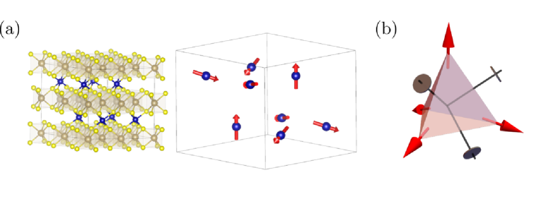
Figure 3: (a) Crystal (left panel) and spin (right panel) structures of CoTa₃S₆. (b) The tetrahedron spanned by four spins in the magnetic structure. The black lines denote the two-fold rotation axes relevant to the spin translation group.

The anomalous Hall response does not suffer from such severe symmetry constraint in the case of the noncoplanar spin configuration because the spin-only group is trivial [Eq. (19)]. It is noteworthy that the nontrivial spin translation symmetry realizes the spin-free orbital polarization. We take a layered material CoTa₃S₆ for an example [69, 70] (Fig. 3). After the computational search for the magnetic symmetry [35], the magnetic space group symmetry is identified to be

$$\mathbf{G}=P32^{\prime}.$$ (50)

The associated SO-coupled magnetic point group $\mathbf{P}=32^{\prime}$ leads to the conclusion that the spin ($\bm{M}_{\text{sp}}$) and orbital magnetization ($\bm{M}_{\text{orb}}$) can concurrently show up along the three-fold rotation axis. Thus, we cannot distinguish the KL and geometrical contributions to the Hall effect within the conventional magnetic point group analysis.

Next, We consider the spin-group symmetry identified by utilizing the method proposed in Ref. [31]. Owing to the noncoplanar spin structure, the spin-only group is trivial and the spin space group is coincident with the nontrivial spin space group, $\mathcal{G}=\overline{\mathcal{G}}$ in Eq. (20). The spin space group is written by the internal semidirect product of the spin translation group $\mathcal{G}_{\text{st}}$ and the remaining part $\mathcal{H}$;

$$\mathcal{G}=\overline{\mathcal{G}}_{\text{st}}\rtimes\mathcal{H}.$$ (51)

Since we are interested in the macroscopic physical property, it is sufficient to take into account the point group symmetry. The point group is obtained from Eq. (51) as

$$\mathcal{P}=\mathcal{P}_{\text{st}}\rtimes\mathcal{P}_{\mathcal{H}}.$$ (52)

The point groups $\mathcal{P}_{\text{st}}$ and $\mathcal{P}_{\mathcal{H}}$ is respectively derived from $\overline{\mathcal{G}}_{\text{st}}$ and $\mathcal{H}$ as in Eq. (24). The spin translation part $\mathcal{P}_{\text{st}}$ gives rise to the spin only point group symmetry written by

$$\mathcal{P}_{\text{st}}=\left\{\left(1,W\right)|W\in\{1,2_{X},2_{Y},2_{Z}\}\right\}.$$ (53)

The point group $222=\{1,2_{X},2_{Y},2_{Z}\}$ is constructed from the orthogonal two-fold rotation axes $(X,Y,Z)$ by which four orientations of Co spins are interchanged [Fig. 3(b)]. The remaining part is

$$\mathcal{P}_{\mathcal{H}}=^{3}6^{m_{(100)}}2^{m_{(010)}}2.$$ (54)

We notice that the six-fold symmetry of the crystal (space group $P6_{3}22$, No. 182) remains in the ordered phase without considering SOC.

We are interested in the spin and orbital magnetization which are related with the KP and geometrical Hall effects, respectively. Then, it is enough to consider the spin and orbital parts projected from $\mathcal{P}$ as in Eqs. (28), (29). The spin part is

$$\mathcal{P}_{\text{sp}}(\mathcal{P})=222\rtimes 3m=\bar{4}3m,$$ (55)

and the orbital part is

$$\mathcal{P}_{\text{orb}}(\mathcal{P})=62^{\prime}2^{\prime}.$$ (56)

The spin translation symmetry of Eq. (53) leads to the cubic symmetry $\mathcal{P}_{\text{sp}}=\bar{4}3m$ in spite of the hexagonal crystal structure of CoTa₃S₆. The spin point group symmetry enhanced by the spin translation symmetry has not been addressed in previous studies of emergent responses. On the other hand, the orbital part manifests the axial symmetry whose rotation axis is $[001]$ similar to the SO-coupled case of Eq. (50). Given that these spin and orbital parts of the spin point group, we identify the allowed spin and orbital magnetization,

$$\bm{M}_{\text{sp}}=\bm{0},~{}\bm{M}_{\text{orb}}\parallel[001].$$ (57)

As a result, the anomalous Hall conductivity vector $\bm{\sigma}^{\text{H}}\parallel[001]$ can appear as well as the orbital magnetization without the help of SOC. Furthermore, the zero spin magnetization follows from the cubic symmetry in the spin space. These properties indicate that the anomalous Hall effect of CoTa₃S₆ can be attributed to the geometrical origin ($\bm{\sigma}^{\text{g}}$) and that the KP contribution ($\bm{\sigma}^{\text{KP}}$) may be suppressed due to vanishing spin polarization. The obtained symmetry argument may be consistent with the recent experimental finding [69].

We have observed two characteristic aspects of spin group symmetry in this section. The spin-only group associated with low-dimensional spin configuration gives rise to strong constraints on the orbital-space objects, which may forbid physical responses unique to the time-reversal-odd phase. On the other hand, the noncoplanar spin structure may lead to such emergent responses while it holds the highly-symmetric spin space due to the spin translation group which instead leads to vanishing responses relevant to the spin degree of freedom instead. These contrasting situations are systematically understood by the spin-group symmetry analysis incorporating more details of spin structures such as spin-structure dimension.

III.3 magnetoelectric effect and spin/orbital magnetic quadrupole moments

The spin-group symmetry analysis distinguishes the role of spin and orbital degrees of freedom in the magnetoelectric effect as it seperately identifies the spin and orbital magnetization as demonstrated Eq. (57). We here consider the correlation between magnetization and electric polarization written by

$$P_{i}=\chi_{ij}^{PM}H_{j},~{}M_{i}=\chi_{ij}^{MP}E_{j}.$$ (58)

The frequency dependence is suppressed. In particular, the reactive term is called magnetoelectric effect and the absorptive term is the inverse magneto-galvanic effect [48, 46] (see also Table 1).

In the following, we focus on the dc magnetoelectric effect $\alpha_{ij}=\chi_{ij}^{MP,\text{rea}}(\omega=0)$, which appears even in systems with no electric conductivity, that is, insulators at the zero temperature. The magnetoelectric effect is further classified into the spin and orbital parts $\alpha_{ij}^{\text{sp}}$, $\alpha_{ij}^{\text{orb}}$ where the spin and orbital magnetization participate in the response, respectively.

Firstly, we consider a prototypical magnetoelectric material Cr₂O₃ [71, 72] [Fig. 4(a)]. Its collinear antiferromagnetic order does not break translation symmetry, and the spin translation group is trivially the translation group without spin-space rotations ($\overline{\mathcal{G}}_{\text{st}}=\mathcal{T}$). Supposing that the spins are aligned to the $[001]$ axis in the spin space, the spin crystallographic point group is

$$\mathcal{P}=\mathcal{P}_{\text{so}}\times\overline{\mathcal{P}},$$ (59)

where the spin-only group $\mathcal{P}_{\text{so}}$ is for the one-dimensional spin configuration [Eq. (17)]

$$\mathcal{P}_{\text{so}}=\text{SO(2)}\rtimes\left\{1,m_{\parallel}\right\}.$$ (60)

The nontrivial spin point group is

$$\overline{\mathcal{P}}=^{\bar{3}}\bar{3}^{m}m.$$ (61)

The spin part associated with $\mathcal{P}$ manifests the centrosymmetric point group symmetry as

$$\mathcal{P}_{\text{sp}}(\mathcal{P})=\text{O(2)}\rtimes\{1,m_{\parallel}\},$$ (62)

and the orbital part is given by a centrosymmetric gray group

$$\mathcal{P}_{\text{orb}}(\mathcal{P})=\bar{3}m1^{\prime},$$ (63)

which differs from the noncentrosymmetric black-white point group under SOC, $\mathbf{P}=\bar{3}^{\prime}m^{\prime}$.

In the framework of spin group symmetry, the symmetry of spin and orbital magnetoelectric effect is determined by Eqs. (59) and (63), respectively. The orbital contribution is absent $\alpha_{ij}^{\text{orb}}=0$ following from either of the space-inversion [$\left(-1,W\right)\in\mathcal{P}$ (det $W=+1$)] or orbital time-reversal symmetry [$\left(1,W\right)\in\mathcal{P}$ (det $W=-1$)]. On the other hand, taking into account the spin-space rotations, the spin point group of Eq. (59) does not preserve the trivial time-reversal or space-inversion symmetry. By the computational symmetry analysis, we found that only the spin contribution $\alpha_{zz}^{\text{sp}}\neq 0$ survives. This is because the spin-only group forbids spin polarization transverse to the collinear axis ($\alpha_{yj}^{\text{sp}},\alpha_{zj}^{\text{sp}}=0$). For comparison, the SO-coupled case with $\mathbf{P}=\bar{3}^{\prime}m^{\prime}$ leads to all the diagonal components $\alpha_{xx},\alpha_{yy},\alpha_{zz}$. Then, only the component $\alpha_{zz}^{\text{sp}}$ corresponding to longitudinal spin polarization can respond to the electric field in the SOC-free manner and is purely ascribed to the spin origin.

Although we assumed the dc case, the result is similarly obtained in the ac case. The ac magnetoelectric effect denoted by $\chi_{ij}^{MP,\text{rea}}(\omega)$ triggers the nonreciprocal optical activity [73, 74, 75]. Owing to the spin group symmetry, the optical activity arises solely from the spin-dipole transition but does not include the orbital-dipole and electric-quadrupole effects in the absence of SOC.

Next, we again consider CoTa₃S₆ to demonstrate the role of spin translation symmetry in the magnetoelectric effect. Similarly to zero spin magnetization, the cubic spin-space symmetry [Eq. (55)] forbids the spin magnetoelectric effect, $\alpha_{ij}^{\text{sp}}=0$. On the other hand, the orbital part of Eq. (56) leads to finite orbital magnetoelectric effects $\alpha_{xy}^{\text{orb}}=\alpha_{yx}^{\text{orb}}$. Then, the magnetoelectric effect of CoTa₃S₆ is summarized as

$$\alpha_{ij}^{\text{sp}}=0,~{}\alpha_{xy}^{\text{orb}}=-\alpha_{yx}^{\text{orb}}\neq 0.$$ (64)

In the SO-coupled point group symmetry of Eq. (50), $\alpha_{xy}=-\alpha_{yx}$ is similarly allowed while the spin contribution participates as well.

The symmetry analysis shows the possibility of the spin-orbit-free magnetoelectric effect dominated by the orbital contribution. Among known mechanisms for the magnetoelectricity [76], the identified response may originate from the exchange striction mechanism [77, 78] and the dynamical phase [79] which do not require SOC. Note that we here discussed the orbital magnetoelectric effect induced by the spin order [80] rather than that what arises from the orbital-current order [81].

We took the overview of the relation between the anomalous Hall effect and orbital magnetization in Sec. III.2. A similar discussion can be found in the case of the magnetoelectricity; the response may be correlated with higher-order anisotropy of magnetic charge, that is, the magnetic quadrupole moment $\mathrm{Q}_{ij}$ [82, 83]. The symmetry of $\mathrm{Q}_{ij}$ is schematically given by the tensor product of the magnetization and position as $\mathrm{Q}_{ij}\sim M_{i}r_{j}$ such as magnetic toroidal moment $\mathrm{Q}_{xy}-\mathrm{Q}_{yx}=\left(\bm{M}\times\bm{r}\right)_{z}$. According to the space-time symmetry, we can find the correspondence between the magnetic quadrupole moments and magnetoelectric effect given by

$$\mathrm{Q}_{ij}\leftrightarrow\alpha_{ij}.$$ (65)

The magnetization $M_{i}$ can be classified into the spin and orbital contributions in terms of the spin group symmetry. Then, the symmetry analysis of the allowed magnetoelectric effect can be reproduced by identifying the relevant spin/orbital magnetic quadrupole moments with the use of Eq. (4). Interestingly, recent theoretical studies identified that the magnetic quadrupole moment [84, 85, 86, 87] covers not only the magnetoelectric effect but also other cross-correlated responses [88].

For instance, let us consider the multipolar degree of freedom corresponding the magnetoelectric effect of CoTa₃S₆. The allowed multipole moment is the orbital toroidal moment $\mathrm{Q}_{xy}^{\text{orb}}-\mathrm{Q}_{yx}^{\text{orb}}$ where the toroidal moment is a polar vector with the odd time-reversal parity. The symmetry of toroidal moment is consistent with that of the orbital magnetoelectric effect [Eq. (64)]. The toroidal moment polarized along the $[001]$ direction can be intuitively understood by its orbital magnetization and crystal structure. The space group symmetry of CoTa₃S₆ (No. 182, $P6_{3}22$) does not comprise any improper rotation symmetry in the orbital space [89], and hence every axial quantity can be coupled to the corresponding polar quantity with preserving the time-reversal parity. In the present case, the orbital magnetization (axial time-reversal-odd vector) is coupled to the orbital toroidal moment (polar time-reversal-odd vector) as in the case of magnetochiral anisotropy [90] [Fig. 4(b,c)]. The coupling between the orbital magnetization and toroidal moment is a consequence of its chiral crystal structure, and the ligands surrounding magnetic Co atoms play essential roles. We checked that the noncoplanar spin structure of Co atoms does give rise to orbital magnetization but have no orbital toroidal moment without Ta and S atoms.

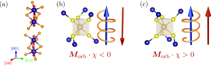
Figure 4: (a) Crystal and spin structures of Cr₂O₃ with collinear axis in the $[001]$ direction. (b,c) Chirality of the crystal structure of CoTa₃S₆ implied by TaS₆ prism with the twisted coordination of Co atoms. The twisting arrangement determines the chirality. When orbital magnetization (blue-colored vector) is formed along the $[001]$ direction due to its noncoplanar spin ordering, (b) the toroidal moment (red-colored vector) is anti-parallel to it, (c) while it is parallel with the opposite chirality.

III.4 Spin Hall response and rotators

Let us consider another spin-related response, electric-field ($E_{j}$) induction of spin-polarized current $J_{i}^{s_{k}}$. The spin-polarized current may be given by $J_{i}^{s_{k}}=\{J_{i},s_{k}\}/2$ which is the product of the spin- and orbital-space objects. The response formula reads

$$J_{i}^{s_{k}}=\sigma_{ij}^{k}E_{j}.$$ (66)

The parity under the time-reversal symmetry is $\theta_{J^{s}}\theta_{E}=+1$, and the electric contribution is reactive while the magnetic is absorptive according to the classification in Sec. III.1. For the dc limit, the electric effect includes the well-known spin Hall effect prominent in the spin-orbit-coupled semiconductors [91, 92], while the magnetic is in magnetic metals as discussed in studies of magnetic spin Hall effect [93, 11, 12, 13, 94, 95]. The absence of SOC and spin order leads to the isotropic spin-space symmetry indicating the vanishing response.

We refer to the symmetry analysis of Refs. [11, 12] and decompose $\sigma_{ij}^{k}$ into the electric and magnetic components. The target material, a noncollinear and coplanar magnet Mn₃Sn, is attracting a lot of attention because of its potential application for spintronics and magneto-optical components [Fig. 5(a)]. The spin crystallographic point group is given by

$$\mathcal{P}=\mathcal{P}_{\text{so}}\times\overline{\mathcal{P}}.$$ (67)

The spin-only group is

$$\mathcal{P}_{\text{so}}=\left\{\left(1,W\right)|W\in\{1,m_{(001)}\}\right\},$$ (68)

for a two-dimensional spin structure. The nontrivial spin point group $\overline{\mathcal{P}}$ is [22]

$$\overline{\mathcal{P}}=^{3}6/^{1}m^{m_{(120)}}m^{m_{(110)}}m,$$ (69)

where the spin configuration is taken to preserve the spin point group symmetry for $g=\left(2_{[100]},2_{[100]}\right)$. The spin part associated with $\mathcal{P}$ is

$$\mathcal{P}_{\text{sp}}(\mathcal{P})=m_{(001)}\times 3m=\bar{6}2m,$$ (70)

and the orbital part is

$$\mathcal{P}_{\text{orb}}(\mathcal{P})=6/mmm1^{\prime},$$ (71)

coinciding with the magnetic point group of the paramagnetic state, while the SO-coupled magnetic point group shows the reduction of its crystal class as $\mathbf{P}=mm^{\prime}m^{\prime}$. Thus, as long as we consider phenomena related to orbital degrees of freedom, the antiferromagnetic state exhibited by Mn₃Sn does not show any symmetry breaking. On the other hand, owing to the spontaneously-emerged anisotropy in the spin space, the electric field can produce rise to the spin-polarized current. The response is explicitly given by

$$\sigma_{xy}^{z}=-\sigma_{yx}^{z},$$ (72)

for the electric contribution and

$$\sigma_{xx}^{x}=\sigma_{xy}^{y}=\sigma_{yx}^{y}=-\sigma_{yy}^{x},$$ (73)

for the magnetic. These spin-orbit-free components may overwhelm those requiring SOC [11, 12].

Following the parallel discussion of the previous sections III.2 and III.3, the symmetry analysis can apply to more complex spin structures and be extended to include the orbital counterpart such as the orbital Hall effect [96, 97]. The orbital counterpart is obtained by using the current whose magnetic polarization is attributed to the orbital origin. For instance, CoTa₃S₆ with the cubic spin-space symmetry [Eq. (55)] indicates the zero spin-related part $\sigma_{ij}^{k,\text{sp}}=0$. The orbital counterpart, however, is allowed even without SOC such as the magnetic contributions $\sigma_{xx}^{z,\text{orb}},\sigma_{yy}^{z,\text{orb}},\sigma_{zz}^{z,\text{orb}}$.

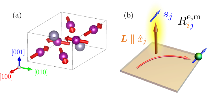
Figure 5: (a) Spin structure of Mn₃Sn. (b) Transverse conversion between the charge and spin currents denoted by the rotator $R_{ij}$. The Hall plane perpendicular to the $x_{i}$ direction is for the current whose spin is polarized along the $x_{j}$ direction in the spin space.

We further consider the equilibrium quantities relevant to the electric/magnetic spin Hall responses by the analogy of the SOC Hamiltonian [43]. In the expression for the atomic SOC of Eq. (14), the orbital momentum $\bm{L}\sim\bm{r}\times\bm{p}$ may be replaced with the cross product of the electric field and current $\bm{E}\times\bm{J}$, since each pair of vectors share the same space-time symmetry. Then, the relativistic spin-orbit interaction has a correspondence with the response as

$$\bm{L}\cdot\bm{s}\sim\left(\bm{J}\times\bm{E}\right)\cdot\bm{s}=\epsilon_{ijk}E_{j}J_{i}s_{k}\leftrightarrow\sigma_{ij}^{k}=\epsilon_{ijk}\sigma_{0},$$ (74)

where $\epsilon_{ijk}\sigma_{0}$ indicates the (electric) spin Hall effect whose spin polarization is perpendicular to the Hall plane defined by the $\bm{E}$ and $\bm{J}$ [Fig. 5(b)]. That is why the spin Hall effect is allowed under the SOC effect. The correspondence between the electric spin Hall effect and the product of $L_{i}$ and $s_{j}$ may be generalized to that in the framework of spin group symmetry. Then, we here introduce the rotator $R_{ij}^{\text{e}}$ giving the transverse correlation between charge and spin currents. The symmetry of $R_{ij}^{\text{e}}$ coincides with the product of the time-reversal-odd ($\theta_{X}=-1$) and axial vectors $R_{ij}^{\text{e}}\sim L_{i}s_{j}$. $L_{i}$ and $s_{j}$ are defined in the orbital and spin space, respectively. The rotator implies the Hall response denoted by the Hall plane perpendicular to the $i$-directed for the $x_{j}$-polarized spin current [Fig. 5(b)],

$$R_{ij}^{\text{e}}\leftrightarrow\epsilon_{iab}\sigma_{ab}^{j}.$$ (75)

Specifically, the trace $\sum_{i}R_{ii}^{\text{e}}$ corresponds to the SOC of Eq. (14). We note that $\sigma_{ab}^{j}$ in the right hand side is the reactive contribution, since the rotator $R_{ij}^{\text{e}}$ totally shows the even parity under the time-reversal operation ($\theta_{L}\theta_{s}=+1$) and therefore indicates the nonmagnetic (electric) spin Hall effect. For instance, referring to the spin crystallographic point group of Mn₃Sn [Eq. (67)], we identify the rotator $R_{zz}^{\text{e}}$ corresponding to the spin Hall response of Eq. (72) where the $z=(001)$ Hall plane is obtained as $(\bm{E}\times\bm{J})_{z}$ and the spin is polarized along the $z$-direction. The nonmagnetic spin Hall effect is a response characteristic of noncollinear spin systems under no SOC effect [12] as we corroborate in Sec. IV.

It is straightforward to similarly derive the quantity relevant to the magnetic spin Hall effect, that is, magnetic rotator $R_{ij}^{\text{m}}\sim\overline{L}_{i}s_{j}$ with the time-reversal-even and axial vector $\overline{L}_{i}$ defined in the orbital space [43]. The rotator $R_{ij}^{\text{m}}$ is time-reversal-odd and corresponds to the magnetic spin Hall effect given by $\epsilon_{iab}\sigma_{ab}^{j}$. In the case of Mn₃Sn, the magnetic rotator is absent without SOC, $R_{ij}^{\text{m}}=0$. This is consistent with the symmetry analysis of Eq. (73) whose field and response can be longitudinal to each other.

IV High-throughput symmetry analysis of spin group symmetry

The computational search for the spin space group symmetry allows us to identify physical properties free from the SOC effect [35, 31]. We present symmetry analysis with dozens of observed spin configurations obtained from magndata [33, 32]. We have performed the symmetry analysis of 1512 magnetic materials which have no site disorder. For the spin-structure dimension, 914 one-dimensional, 403 two-dimensional, and 195 three-dimensional systems are studied. The magnetic materials are numbered by following the identification number provided in magndata such as Cr₂O₃ (# 0.59).

In this section, we discuss the physical quantities such as spin/orbital magnetization and magnetic quadrupole moments, and electric/magnetic rotators introduced in Sec. III to investigate spin-orbit-free physical phenomena. Providing some examples of spin space group ($\mathcal{G}$) with comparison to the analysis with magnetic space group ($\mathbf{G}$), we investigate characteristic physical properties in the viewpoint of symmetry.

IV.1 Spin crystallographic symmetry

Let us classify the magnetic materials in terms of the spin crystallographic or magnetic space group symmetry. Since the spin space group comprises its corresponding magnetic space group as a subgroup, the orders of groups satisfies the relation $|\overline{\mathcal{G}}|/|\mathbf{G}|\in\mathbb{N}=\{1,2,3,\cdots\}$ where we consider the nontrivial spin space group $\overline{\mathcal{G}}$ instead of $\mathcal{G}$. Figure 6 illustrates how many symmetries are restored by neglecting SOC. For instance, the maximal symmetry restoration occurs in the case of a noncoplanar magnet CrSe (# 2.35) [98]. The hexagonal crystalline symmetry (space group No. 194, $P6_{3}/mmc$) is intact for the spin space group $\mathcal{G}$, while the crystal class is reduced to the trigonal for the magnetic space group $\mathbf{G}$. The spin translation group as large as $|\overline{\mathcal{G}}_{\text{st}}|=3$ also contributes to the higher symmetry of $\overline{\mathcal{G}}$ [31].

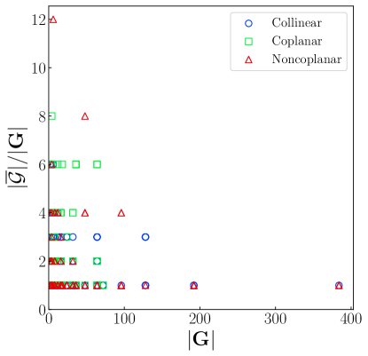
Figure 6: Distribution of magnetic materials parametrized by the order of the magnetic space group ($|\mathbf{G}|$) and by the ratio between the order of the nontrivial spin space group ($|\overline{\mathcal{G}}|$) and $|\mathbf{G}|$. The distributions are categorized based on whether the spin-structure dimension is collinear, coplanar (but noncollinear), or noncoplanar.

For a more detailed comparison, we classify the orbital symmetry of the spin point group ($\mathcal{P}_{\text{orb}}$) and of the SO-coupled magnetic point group ($\mathbf{P}$) in terms of the anti-unitary symmetry such as colorless, gray, and black-white groups. Owing to the spin-only group, the low-dimensional spin structure ($\mathcal{D}_{\text{sp}}=1,2$) makes the orbital-space symmetry $\mathcal{P}_{\text{orb}}$ gray-type irrespective of its SO-coupled magnetic point group symmetry [Eq. (23) for $\mathcal{D}_{\text{sp}}=1$ and Eq. (67) for $\mathcal{D}_{\text{sp}}=2$]. On the other hand, the noncoplanar system ($\mathcal{D}_{\text{sp}}=3$) can be characterized by any of three different types of magnetic point groups. Table 2 shows the classification result. The absence of the SOC constraint [Eq. (15)] allows for the additional anti-unitary symmetry and hence some of the colorless groups among $\mathbf{P}$ are turned into gray groups for the classification of $\mathcal{P}_{\text{orb}}$.

Table 2: Classification table of the spin point group and SO-coupled magnetic point group for the noncoplanar magnets in the light of anti-unitary symmetry.

	Colorless	Gray	Black-White
$\mathbf{P}$	46	46	103
$\mathcal{P}_{\text{orb}}$	42	46	107

We take some examples to compare the magnetic symmetry with and without SOC. For an example of low-dimensional spin structures, we consider a coplanar magnet Ba₃MnSb₂O₉ (# 1.0.46). The material crystalizes in the structure denoted by the centrosymmetric space group $C2/m$ (No. 15) [99], and its coplanar spin structure ($\mathcal{D}_{\text{sp}}=2$) is formed by magnetic moments at Mn atoms [Fig. 7(a)]. No anti-unitary symmetry exists in the magnetic space group $\mathbf{G}=C2$ (type I) allowing for both of ferroelectric and ferromagnetic polarizations. On the other hand, such multiferroic property vanishes if there exists no SOC effect. The spin space group reads

$$\mathcal{G}=\mathcal{G}_{\text{so}}\times\overline{\mathcal{G}}.$$ (76)

The two-dimensional spin structure corresponds to the spin-only group

$$\mathcal{G}_{\text{so}}=\{\left((1,\bm{0}),1\right),~{}\left((1,\bm{0}),m_{(001)}\right)\},$$ (77)

and the nontrivial part $\overline{\mathcal{G}}$ is isomorphic to the space group $C2/m$. $\overline{\mathcal{G}}$ is generated by

$$\left((1,\bm{t}),1\right),\left((-1,\bm{0}),m_{(010)}\right),~{}\left((2_{[010]},\bm{t}^{\prime}),m_{(100)}\right)\in\overline{\mathcal{G}},$$ (78)

in addition to the trivial translation operations associated with the monoclinic crystal structure. We here introduced the translations $\bm{t}=[0.5,0.5,0]$ and $\bm{t}^{\prime}=[0,0,0.5]$. When $\mathcal{G}$ is reduced to the spin crystallographic point group $\mathcal{P}$, the orbital part of $\mathcal{P}$ is centrosymmetric and gray as

$$\mathcal{P}_{\text{orb}}(\mathcal{P})=2/m1^{\prime},$$ (79)

in contrast to the SO-coupled case ($\mathbf{P}=2$). Consequently, the spin group symmetry forbids various physical phenomena activated by the time-reversal or space-inversion symmetry breaking.

Next, we consider a noncoplanar magnet Mn₃CuN (# 2.5) [100]. The complex spin structure consists of magnetic moments at Mn atoms having two different moduli [Fig. 7(b)]. The magnetic space group is

$$\mathbf{G}=P4/m,$$ (80)

from which the magnetic point group is $\mathbf{P}=4/m$. Thus, owing to the spin order and SOC, the cubic crystalline symmetry (space group No. 221, $Pm\bar{3}m$) is reduced to the tetragonal. The magnetic symmetry allows for the magnetization along the $[001]$ axis.

Then, let us consider its spin space group symmetry. Owing to the finite propagation vector of the order parameter, the spin space group includes the spin translation group $\overline{\mathcal{G}}_{\text{st}}$ generated by

$$\left((R,\bm{t}),W\right)=\left((1,\bm{t}),2_{z}\right)$$ (81)

with $\bm{t}=(0.5,0.5,0)$ and by trivial translation operations without any spin-space rotations. Then, we obtain the coset decomposition of the spin space group as

$$\mathcal{G}=\bigcup_{i}g_{i}\,\overline{\mathcal{G}}_{\text{st}},$$ (82)

where the representative operations $g_{i}$ are taken by

$$\left((R,\bm{t}),W\right)=\left((-1,\bm{0}),1\right),~{}\left((4^{+}_{[001]},\bm{0}),4^{+}_{[001]}\right),~{}\left((m_{(010)},\bm{0}),m_{\alpha}\right),~{}\left((m_{(100)},\bm{0}),m_{\beta}\right).$$ (83)

The mirror operation $W=m_{\alpha}$ is depicted in Fig. 7(c). Importantly, the spin-space-group operations related to $m_{\alpha},m_{\beta}$ are preserved without the SOC condition of Eq. (15) and makes the orbital-space symmetry twin-colored. The spin point group is obtained as

$$\mathcal{P}=^{2_{[001]}}1^{4_{[001]}}4/^{1}m^{m_{\beta}}m^{m_{\gamma}}m,$$ (84)

with the spin-space mirror operation $W=m_{\gamma}$ associated with the orbital-space mirror reflection $R=m_{(1\bar{1}0)}$. Accordingly, we obtain

$$\mathcal{P}_{\text{sp}}=4mm,$$ (85)

for the spin part, and

$$\mathcal{P}_{\text{orb}}(\mathcal{P})=4/mm^{\prime}m^{\prime},$$ (86)

for the orbital part. The resulting orbital-space symmetry of $\mathcal{P}_{\text{orb}}$ differs from the colorless magnetic point group $\mathbf{P}=4/m$ for the SO-coupled case.

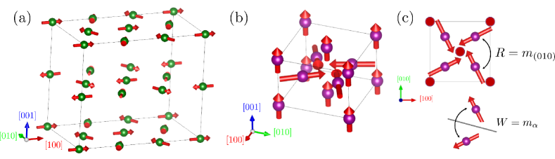
Figure 7: Spin configurations of (a) Ba₃MnSb₂O₉ with only Mn atoms and of (b,c) Mn₃CuN. In (c), the symmetry for the spin space operation $\left((m_{(010)},\bm{0}),m_{\alpha}\right)$ is depicted. The mirror operations $W=m_{\beta},m_{\gamma}$ can be similarly obtained.

IV.2 Emergent physical properties

IV.2.1 Magnetization

Here we consider the spin and orbital magnetization arising from the spin ordering. Although the uniform spin magnetization trivially appears in the ferromagnetic materials, the orbital counterpart is severely forbidden due to the spin-only group of simple spin structures such as collinear and coplanar configurations (see Sec. III.2). Then, we focus on the 195 noncoplanar magnets which may possess orbital magnetization. We show the classification concerning magnetization in Table 3. The classification also covers the magnetization identified by the magnetic symmetry ($\mathbf{G},\mathbf{P}$) including the SOC effect, that is, the spin-orbital-entangled magnetization denoted by $\bm{M}_{\text{SOC}}$. When either non-zero spin or orbital magnetization is present in a given spin space group, $\bm{M}_{\text{SOC}}$ is similarly allowed due to the group-subgroup relation of $\mathbf{G}<\mathcal{G}$. Then, we classify the noncoplanar magnets into five classes in terms of magnetization.

The system with orbital-free spin magnetization (Class M2 of Table 3) is trivial since such kind of materials can be found in typical ferromagnetic materials. On the other hand, the spin-free orbital magnetization (Class M3) indicates a nontrivial spin group symmetry hosting the orbital magnetization not to be concomitant with spin magnetization. The materials of Class M3 are as follows; DyCrWO₆ (# 0.316), CuB₂O₄ (# 0.431), Fe₃F₈(H₂O)₂ (# 2.61), TbCrO₃ (# 2.62), DyCrO₃ (# 2.63, # 2.64), and MgCr₂O₄ (# 3.4). The candidate materials are mostly insulators in contrast to the noncoplanar magnetic metal CoTa₃S₆ discussed in Sec. III.2. Thus, they may not be promising candidates for the geometrical Hall effect, whereas the orbital magnetization should participates in similar phenomena for quasiparticles conductive in electrically-insulating materials such as phonon and magnon [101]. The orbital magnetization also plays an important role in various magneto-optical phenomena such as Faraday rotations [102]. Interestingly, the optical response may be tolerant to extrinsic effects such as skew scattering yielding anomalous Hall effect [23] and hence it can be a good testbed for investigating the intrinsic role of the orbital magnetization in emergent responses.

We observe that CrSe (# 2.35) shows the magnetization if and only if SOC is taken into account (Class M4). This is because the cubic symmetry of spin space group $\mathcal{G}$ is reduced to the trigonal magnetic point group under SOC.

We also notice that the spin and orbital contributions to the equilibrium properties may be distinguished even when both are allowed such as in Class M1 of Table 3. As an example for Class M1 of Table 3, the spin group symmetry of Mn₃O₄ (# 2.52) leads to the spin and orbital magnetization given by

$$\bm{M}_{\text{sp}}\parallel[010],~{}\bm{M}_{\text{orb}}\parallel[001].$$ (87)

The two perpendicular magnetizations get entangled with each other under the SOC effect, and the magnetization can be in the $(100)$ plane. Note that we cannot determine the relative orientation of spin space axes with respect to the orbital-space coordinate system without SOC. We, however, determined the spin-space axes of Eq. (87) by referring to the spin configuration observed in experiments, and thus the peculiar relation between spin and orbital magnetization may give an implication; e.g., the anomalous Hall effect $\sigma_{xy}=-\sigma_{yx}$ may be larger than the other $\sigma_{zx}=-\sigma_{xz}$, because the former is due to the orbital magnetization $\bm{M}_{\text{orb}}\parallel[001]$ while the latter results from a weak SOC effect of Mn atoms.

Table 3: Classification of noncoplanar magnetic materials in terms of spin and orbital magnetization $\bm{M}_{\text{sp}},\bm{M}_{\text{orb}}$. $\bm{M}_{\text{SOC}}$ denotes the magnetization under the SOC effect. “Num.” denotes the number of data of magnetic materials belonging to each class.

	$(\bm{M}_{\text{sp}},\bm{M}_{\text{orb}},\bm{M}_{\text{SOC}})$	Num.
M1	$(\bigcirc,\bigcirc,\bigcirc)$	69
M2	$(\bigcirc,\times,\bigcirc)$	2
M3	$(\times,\bigcirc,\bigcirc)$	7
M4	$(\times,\times,\bigcirc)$	1
M5	$(\times,\times,\times)$	117
Total		195

Finally, we comment on the relation between Class M2 and the spin scalar chirality. The noncoplanar nature, indispensable for the orbital magnetization and geometrical Hall effect, can be quantified by the spin scalar chirality vector $\bm{C}$

$$C_{i}=\int d\bm{r}\epsilon_{ijk}\bm{s}(\bm{r})\cdot\left[\frac{\partial}{\partial r_{j}}\bm{s}(\bm{r})\times\frac{\partial}{\partial r_{k}}\bm{s}(\bm{r})\right],$$ (88)

which has the same spin-orbital symmetry as that of the orbital magnetization $\bm{M}_{\text{orb}}$. The importance of the spin scalar chirality has been explored in various materials such as Kagomé lattice [26, 27, 68, 103] and magnetic skyrmion crystals [28, 29]. The spin scalar chirality may be defined in a lattice system as

$$\overline{C}_{a}=\sum_{\triangle}\bm{S}_{i}\cdot\left(\bm{S}_{j}\times\bm{S}_{k}\right)\left(\left\{i,j,k\right\}\in\triangle\right),$$ (89)

where three spins spanning the triangle ($\triangle$) are in the same plane normal to the $x_{a}$ axis [Fig. 8(a)] [104]. Let us consider the noncoplanar magnet MgCr₂O₄ (# 3.4) [105]. The spin moments dwelling on Cr atoms show the coplanar structure in each of $[001]$-stacked planes [Fig. 8(b)]. Thus, no matter how we take a triangle unit, the system has no spin scalar chirality defined by Eq. (89). On the other hand, the orbital magnetization $\bm{M}_{\text{orb}}$ and spin scalar chirality $\bm{C}$ in continuum space is identified to be along the $[001]$ direction according to our computational methods. It implies that our symmetry analysis unambiguously identifies the geometrical Hall effect for complex magnetic materials whose spin chirality may hard to identify.

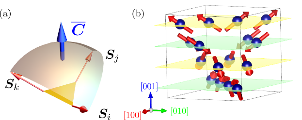
Figure 8: (a) Spin scalar chirality vector $\overline{\bm{C}}$ in a lattice system defined by the three noncoplanar spins within the same plane. (b) Spin structure of MgCr₂O₄. Only the magnetic atoms (Cr) are shown. The noncoplanar spin structure is decomposed into the coplanar spin structure stacked along the $[001]$ direction. The discrete spin scalar chirality $\overline{C}_{[001]}$ is zero for each plane (yellow- or green-colored plane)

IV.2.2 Magnetic quadrupole moment

We consider the spin and orbital quadrupole moments $\mathrm{Q}_{ij}^{\text{sp}},~{}\mathrm{Q}_{ij}^{\text{orb}}$. While the orbital contribution similarly does not appear without a noncoplanar spin structure, the low-dimensional spin structures are of interest due to the spin contribution. Furthermore, we can gain insight into relativistic effects on the quadrupole-mediated physical responses such as the magnetoelectric effect from the comparison between the magnetic quadrupole moments with and without SOC. We therefore categorize the magnetic materials by the spin/orbital/spin-orbital-coupled ($\mathrm{Q}_{\text{SOC}}$) quadrupole moments and their spin-structure dimension (Table 4).

Table 4: Classification of magnetic quadrupole moments. The spin ($\mathrm{Q}_{\text{sp}}$), orbital ($\mathrm{Q}_{\text{orb}}$), and spin-orbital-coupled contributions ($\mathrm{Q}_{\text{SOC}}$) are classified by the spin-structure dimension ($\mathcal{D}_{\text{sp}}=1,2,3$).

	$(\mathrm{Q}_{\text{sp}},\mathrm{Q}_{\text{orb}},\mathrm{Q}_{\text{SOC}})~{}~{}~{}$	$\mathcal{D}_{\text{sp}}$
		1	2	3
Q1	$(\bigcirc,\bigcirc,\bigcirc)$	0	0	42
Q2	$(\bigcirc,\times,\bigcirc)$	142	94	0
Q3	$(\times,\bigcirc,\bigcirc)$	0	0	4
Q4	$(\times,\times,\bigcirc)$	93	24	1
Total		235	212	47

To be consistent with the spin-only group for the spin-structure dimension $\mathcal{D}_{\text{sp}}=1$ and $2$, the quadrupole moments originate from only the spin degree of freedom (Class Q2) without SOC, while both spin and orbital contributions are admixed (Class Q1) in noncoplanar case ($\mathcal{D}_{\text{sp}}=3$). Interestingly, only the orbital quadrupole moment is allowed in the spin-orbit-free manner (Class Q3) for U₃As₄ (# 0.169), U₃As₄ (# 0.170), CrSe (# 2.35), MgCr₂O₄ (# 3.4). It is noteworthy that the noncoplanar magnet CrSe possesses the orbital quadrupole moment without any uniform magnetization (Class M5 of Table 3). The Class Q4 of Table 4 indicates the system whose magnetic quadrupole moment appears if and only if SOC is included. The magnetoelectric property is not kept without SOC in some collinear antiferromagnets because of strong constraints from the spin-only group.

The magnetoelectric effect related to magnetic quadrupole moment has been intensively studied mainly with collinear magnets [46] and with incommensurate magnetic systems [106, 76]. It, however, has been rarely explored for commensurate but noncollinear magnetic structures such as what solely manifests the orbital magnetoelectric effect [107, 80, 108]. Thus, the present classification may lead us to a deep comprehension of the relation between the spin-structure dimension and magnetoelectric effect.

IV.2.3 Rotators for the spin-polarized current responses

Finally, let us consider the electric and magnetic spin-current rotators $R_{ij}^{\text{e,m}}$. These quantities comprise the spin degree of freedom in $j$-th component of $R_{ij}$ and vanishes in the paramagnetic state without SOC. Under the SOC effect, the electric rotator $R_{ij}^{\text{e}}$ is trivially induced in every system, while the magnetic rotator $R_{ij}^{\text{e}}$ requires the time-reversal symmetry breaking . Then, we identify candidate materials possessing the electric rotator without SOC ($R_{ij}^{\text{e}}$), magnetic rotator without SOC ($R_{ij}^{\text{m}}$), and magnetic rotator under the SOC effect ($R_{ij}^{\text{mS}}$) for each spin-structure dimension (Table 5).

Table 5: Classification of the spin current rotators. Magnetic material data with the spin-structure dimension $\mathcal{D}_{\text{sp}}=1,2,3$ are classified by the electric ($R_{\text{e}}$), magnetic ($R_{\text{orb}}$), and SO-coupled magnetic rotators ($R_{\text{mS}}$).

	$(R_{\text{e}},R_{\text{m}},R_{\text{mS}})~{}~{}~{}$	$\mathcal{D}_{\text{sp}}$
		1	2	3
R1	$(\bigcirc,\bigcirc,\bigcirc)$	0	115	100
R2	$(\times,\bigcirc,\bigcirc)$	130	19	0
R3	$(\times,\times,\bigcirc)$	123	42	5
R4	$(\bigcirc,\times,\times)$	0	164	79
R5	$(\bigcirc,\times,\bigcirc)$	0	5	4
Total		253	345	188

For the collinear case ($\mathcal{D}_{\text{sp}}=1$), the electric rotator vanishes due to the spin-only group symmetry ($R_{\text{e}}=0$), but the magnetic contribution is allowed (Class R2 and R3). As a result, the spin Hall effect of collinear magnets is generically attributed to the magnetic origin and hence is unique to magnetic metals. In particular, the candidates for Class R2 may show a sizable spin Hall effect without the help of SOC [12]. It is noteworthy that the spin current induced by the magnetic spin Hall effect is not accompanied by the charge current in the collinear and coplanar magnets due to the absence of the anomalous Hall effect without SOC. This situation is distinct from the Hall effect of SO-coupled systems where the magnetic spin Hall current is admixed with the charge Hall current [14].

For coplanar and noncoplanar magnets ($\mathcal{D}_{\text{sp}}=2,3$), both the electric and magnetic rotators are not forbidden in general. As in the case of Mn₃Sn, the electric rotator can appear in a lot of magnetic materials in a SOC-free manner. On the other hand, to be different from the collinear case, the magnetic rotator rarely appears without being admixed with the electric rotator (Class R2 and R3), because a complex spin structure providing the magnetic rotator secondarily induces the time-reversal symmetric spin-charge anisotropy as well.

We note that the symmetry analysis refers to the spin structures reported in experiments, that is, the spin configurations including the SOC effect such as small canting by the Dzyaloshinskii-Moriya interaction. To obtain a proper insight into the SOC-free responses, we have to remove the SOC corrections by performing the comparative first principle study with and without the SOC effect [109, 110].

V Discussion and Summary

We mainly focused on linear responses such as anomalous Hall, magnetoelectric, and spin Hall responses. The powerful feature, such as electric-magnetic decomposition and classification in terms of spin and orbital degrees of freedom, works in analyzing nonlinear responses as well. We exemplify it by nonreciprocal dc current-induction of CoTa₃S₆. The response reads

$$J_{i}(\omega=0)=\sigma_{i;jk}E_{j}(\omega_{0})E_{k}(-\omega_{0}).$$ (90)

This is called photocurrent response for $\omega_{0}\neq 0$ [111] or nonreciprocal conductivity for $\omega_{0}=0$ [112]. Performing the electric and magnetic decompositions, we obtain the allowed components

$$\sigma_{z;xy}=-\sigma_{z;yx},~{}\sigma_{y;zx}=-\sigma_{y;xz},~{}\sigma_{x;yz}=-\sigma_{x;zy},$$ (91)

for the electric contribution and

$$\sigma_{z;xx}=\sigma_{z;xx},~{}\sigma_{x;zx}=\sigma_{y;zy},~{}\sigma_{x;xz}=\sigma_{y;yz},~{}\sigma_{z;zz},$$ (92)

for the magnetic. Although the electric components are trivially allowed due to the noncentrosymmetric crystal structure of CoTa₃S₆, the magnetic component is correlated with emergence of the orbital magnetic toroidal moment [see Sec. III.3 and Fig. 4(b)] [90, 113, 114, 115]. This implies the giant nonlinear response driven by the nonrelativistic spin-charge coupling [17].

We can separate the spin and orbital contributions to the magnetization-related nonlinear responses. By replacing the dc electric current of Eq. (90) with the spin-/orbital-polarized dc current $J_{i}^{s_{a}}$/$J_{i}^{L_{a}}$, the symmetry analysis can apply to the nonreciprocal spin/orbital current induction $\sigma_{i;jk}^{a,\text{sp}}$/$\sigma_{i;jk}^{a,\text{orb}}$. Owing to the nontrivial spin translation symmetry of Eq. (53), the spin part vanishes ($\sigma_{i;jk}^{a,\text{sp}}=0$) but the orbital contribution survives ($\sigma_{i;jk}^{a,\text{orb}}\neq 0$). The situation is different from that considered in the previous study of the spin contribution [116].

Our work provides a systematic tool for investigating SOC-free responses, whereas it does not address quantitative aspects of responses within the symmetry analysis. Previous studies reported that the spin-orbit-free physical response can be sizable such as spin-polarized current induction [12, 15] and piezomagnetic effect [18], but criteria for identifying giant spin-driven phenomena remain elusive. These problems may be addressed in future works as guided by our symmetry analysis. For instance, the classification of the magnetic quadrupole moments (Table 4) may motivate us to revisit the magnetoelectric effect. Historically, the effect has been mainly explored with simple and collinear magnets such as Cr₂O₃. For collinear magnets without SOC, the one-dimensional spin-only group allows for only the longitudinal magnetoelectric effect where induced magnetization is collinear with the spins. Given that small longitudinal spin fluctuations suppress the magnetoelectric effect at the low temperature [73], the SOC-free magnetoelectric effect is typically small for the collinear magnets. On the other hand, coplanar and noncoplanar magnetic materials may host significant magnetoelectric responses due to remaining spin fluctuations. Although the importance of the noncollinear property has been highlighted by prior theoretical studies [80], candidate materials are not fully explored. The developed spin-group symmetry analysis incorporated into the computational design of magnetic materials [109] may facilitate further investigations into complex spin structures enhancing magnetoelectric responses.

Previous theoretical studies investigated the spin-momentum coupling originating from the spin ordering without the SOC effect [117, 5, 6, 118, 7]. The purpose of this paper is to clarify the macroscopic physical properties in terms of the spin-space-group symmetry, and the spin-group analysis of the spin-splitting structure is beyond our scope. The systematic classification, however, can be similarly obtained by combining the spin-space-group symmetry with spin-momentum-locking classification in the light of multipolar degrees of freedom [41, 42, 43]. By properly taking the characteristics of the spin space group, we can get accurate criteria for spontaneous spin-momentum splitting [119].

To summarize, we established the spin-group symmetry analysis applicable to complex spin structures such as what has a nontrivial spin translation symmetry. Our symmetry analysis is powerful to develop further understandings of spin-order-induced emergent responses and relativistic corrections to them in various magnetic materials. In stark contrast to the widely-adopted magnetic space group, the spin space group takes into account the spin-structure dimension and conveniently allows us to identify the geometric contributions to physical responses such as anomalous Hall and magnetoelectric effects. The spin space group symmetry and characteristic physical responses are automatically identified by our computational methods developed in Ref. [31] and in this work. Performing the computational classification of dozens of magnetic materials, we systematically identified intriguing systems such as what hosts pure orbital magnetization, pure magnetic quadrupole-polarization, and the electric/magnetic spin Hall effect. The developed symmetry analysis will deepen our understanding of spin-orbit-free phenomena by combining first-principle material design.

The program of searching the symmetry-adapted tensors with a given spin space group is on the basis of spglib [34, 35] and spinspg [31], and it is distributed under the BSD 3-clause license.

Note added—

After finalizing the manuscript, we noticed Refs. [120, 121, 122] relevant to our work. These works similarly worked on the identification and classification of spin space groups.

Appendix A Notes on group theory

A.1 General properties of group theory

The terminology used in the paper is briefly mentioned to make the paper self-contained. Let $g=\left(h,W\right),g^{\prime}=\left(h^{\prime},W^{\prime}\right)$ be operations of the spin space group $\mathcal{G}$, the multiplication law is defined as

$$g\cdot g^{\prime}=\left(h\cdot h^{\prime},W\cdot W^{\prime}\right),$$ (93)

where the multiplication of the spin- and orbital-space operations are similarly defined in that for the O(3) group and for the space group, respectively. Accordingly, the spin space group satisfies the group axioms, that is, associativity ($g\cdot g^{\prime}\in\mathcal{G}$), the existence of identity (id.) operation (for $\text{id.}\in\mathcal{G}$, $g\cdot\text{id.}=\text{id.}\cdot g=g$), and the existence of the inverse operation (for $g\in\mathcal{G}$, there uniquely exists the operation $g^{-1}\in\mathcal{G}$ such that $g\cdot g^{-1}=g^{-1}\cdot g=\text{id.}$). We denote $|G|$ as the order of a group $G$ (the number of operations in $G$).

Let $H$ be a group whose all the operations are in $G$, and the group-subgroup relation holds as $H\leq G$. In particular, if there exists $g\in G$ such that $g\not\in H$, the group $H$ is a proper subgroup of $G$ written as $H<G$. Let us consider the subgroup $H$ commuting with every operation of its supergroup $G$ as

$$g\in G,~{}gH=Hg,$$ (94)

then $H$ is a normal subgroup of $G$ written by

$$H\triangleleft G.$$ (95)

A trivial normal subgroup is $G$ itself ($G\triangleleft G$).

The group-subgroup relation indicates that the group $G$ can be decomposed by its subgroup $H<G$ as

$$G =g_{1}H\cup g_{2}H\cup\cdots\cup g_{n}H,$$ (96)

$$=\bigcup_{i}g_{i}H,$$ (97)

in which $g_{i}\in G$ but $g_{i}\not\in g_{j}H$ ($i=1,2,\cdots,n$ and $j=1,2,\cdots,i-1$). The decomposition is similarly performed from the left-hand side as

$$G=\bigcup_{i}H\,\overline{g}_{i}.$$ (98)

As a special case, if $H\triangleleft G$ holds, two-fold decompositions coincide with each other. In that case, the representative operations $\{g_{i}\}$ form the group $G/H$ called the factor group. The factor group is defined by the following multiplication law

$$g_{i}H\cdot g_{j}H=(g_{i}g_{j})H\in G/H.$$ (99)

While the representative operations of the factor group $\{g_{i}\}$ themselves do not form a group in general, there can exist the group $K=\{g_{i}\}$ satisfying the group axiom such as $g_{i}\cdot g_{j}\in K$. Accordingly, $G$ is recast as the internal semidirect product of $H$ and K,

$$G=H\rtimes K,$$ (100)

where $H,K<G$ , $H\triangleleft G$, and there exists the trivial intersection between $H$ and $K$ as $K\cap H=\{\text{id.}\}$. If we further demand the relation $K\triangleleft G$, the group $G$ is given by the (internal) direct product

$$G=H\times K.$$ (101)

When we have the internal semidirect product $G=H\rtimes K$, the operations in $G$ can be written as

$$G=\left\{h\cdot k|h\in H,~{}k\in K\right\}.$$ (102)

In particular, if $G=H\times K$, operations $h\in H$ and $k\in K$ commute with each other.

A.2 Group structure of spin space group

The entire group can be rewritten as the internal direct product by using the spin-only group $\mathcal{G}_{\text{so}}$ as [38]

The spin space group $\mathcal{G}$ has a hierarchical structure given as follows [38].

$$\mathcal{G}=\mathcal{G}_{\text{so}}\times\overline{\mathcal{G}}.$$ (103)

After decomposition, the nontrivial spin space group $\overline{\mathcal{G}}$ is obtained. By taking the trivial point group operation in the orbital space ($R=1$), we obtain a normal subgroup of the nontrivial spin space group defined by

$$\overline{\mathcal{G}}_{\text{st}}=\left\{\left((1,\bm{t}),W\right)|\left((1,\bm{t}),W\right)\in\overline{\mathcal{G}}\right\},$$ (104)

which includes the translation operations without the spin rotation ($W=1$). We call $\overline{\mathcal{G}}_{\text{st}}$ the nontrivial spin translation group. Using the relation $\overline{\mathcal{G}}\triangleright\overline{\mathcal{G}}_{\text{st}}$, we get a coset decomposition

$$\overline{\mathcal{G}}=\bigcup_{i}g_{i}\,\overline{\mathcal{G}}_{\text{st}}.$$ (105)

The nontrivial spin space group is not always given by the internal semidirect product. For instance, $\overline{\mathcal{G}}$ in Eq. (82) cannot be given by such a product. On the other hand, it may be given by such form in some cases [CoTa₃S₆ of Eq. (51)]. See also Ref. [31].

The representative operations for the factor group $\overline{\mathcal{G}}/\overline{\mathcal{G}}_{\text{st}}$ are $g=\left((R,\bm{t}),W\right)$ such that $R\neq 1$ otherwise $g=\text{id.}$. Then, the factor group is isomorphic to a nontrivial spin point group $\overline{\mathcal{P}}$ [39, 22] defined by

$$\overline{\mathcal{P}}=\{\left(R,W\right)|\text{if }W\neq 1,~{}R\neq 1\}.$$ (106)

We can introduce the spin translation group for a given spin space group $\mathcal{G}$ as

$$\mathcal{G}_{\text{st}}=\left\{\left((1,\bm{t}),W\right)|\left((1,\bm{t}),W\right)\in\mathcal{G}\right\},$$ (107)

by which we obtain the relation $\mathcal{G}_{\text{st}}=\mathcal{G}_{\text{so}}\times\overline{\mathcal{G}}_{\text{st}}$. Since the relation $\mathcal{G}_{\text{st}}\triangleleft\mathcal{G}$, we similarly derive the coset decomposition

$$\mathcal{G}=\bigcup_{i}g_{i}\,\mathcal{G}_{\text{st}}.$$ (108)

In the main text, we discuss $\overline{\mathcal{G}}_{\text{st}}$ and simply refer to it as the spin translation group.

A.3 Conventional classification of magnetic symmetry

The magnetic space and point groups account for the magnetic symmetry of nonmagnetic and magnetic systems. In the following, we consider widely-used magnetic symmetry, that is, what with the SOC constraint. The group comprises symmetry operations with and without the time-reversal operation which are respectively unitary and anti-unitary, while it has only unitary operations in some cases. In particular, when there exists an anti-unitary symmetry in group $G$, $G$ has a normal subgroup $H$ consisting of only unitary operations whose order is half that of $G$ ($|H|=|G|/2$). Then, we obtain the coset decomposition

$$G=H\cup aH,$$ (109)

where $a\not\in H$ is an anti-unitary operation including the time-reversal operation $\theta$. Otherwise, the group is formed by only the unitary operations. In terms of anti-unitary symmetry, magnetic symmetry is classified as follows.

Magnetic point group

The magnetic point group is comprised of orbital-space unitary operations ($R$) and anti-unitary operations ($R^{\prime}=\theta R$) where $R$ belongs to the O(3) group. The magnetic point group $\mathbf{P}$ is classified into three types;

Colorless group

no anti-unitary operation in $\mathbf{P}$,

Gray group

trivial anti-unitary symmetry holds as $1^{\prime}=\theta\in\mathbf{P}$,

Black-White group

otherwise ($a=R^{\prime}$ with $R\neq 1$ in Eq. (109)).

Magnetic space group

The magnetic space group $\mathbf{G}$ is formed by the point-group operation $R$ ($R^{\prime}$) without (with) the time-reversal operation and by the translation operation $\bm{t}$. These two operations are frequently summarized to the Seitz notation such as $(R,\bm{t}).~{}(R^{\prime},\tilde{\bm{t}})$.

Similarly to the magnetic point group, the magnetic space group is classified into the four types by its anti-unitary symmetry [39].

Type I

no anti-unitary operation in $\mathbf{G}$,

Type II

trivial anti-unitary symmetry holds as $(1^{\prime},\bm{0})\in\mathbf{G}$,

Type III

$a=(R^{\prime},\bm{t})$ with $R\neq 1$ in Eq. (109),

Type IV

$a=(1^{\prime},\tilde{\bm{t}})$ with $\tilde{\bm{t}}\not\equiv\bm{0}$ (mod centering vectors) in Eq. (109).

Appendix B Canonical correlation for linear response theory and its symmetry constraint

Let us introduce the linear response function of $X_{i}=\chi_{ij}^{XY}F_{j}^{(Y)}$ defined in Eq. (33) in the frequency domain as

$$\chi_{ij}^{XY}(\omega)=\int_{0}^{\infty}dte^{i\omega t-\eta t}\chi_{ij}^{XY}(t),$$ (110)

with the infinitesimal positive parameter $\eta=+0$ building the causality into the response. The response function in the time domain can be written as the form of canonical correlation as [44]

$$\chi_{ij}^{XY}(t)\equiv\kappa_{ij}^{X\dot{Y}}=\int_{0}^{1/T}d\tau\text{Tr}\left[\rho_{\text{eq}}\dot{Y}(-i\tau)X(t)\right].$$ (111)

The operators are in the Heisenberg representation, $X(t)=e^{iHt}Xe^{-iHt}$ with the unperturbed Hamiltonian $H$. We also introduced the temperature $T$ and the density operator for the (unperturbed) equilibrium state $\rho_{\text{eq}}=e^{-H/T}/\text{Tr}\left[e^{-H/T}\right]$. Following Ref. [45], the transformation property of the canonical correlation function (in the frequency domain) is

$$\kappa_{ij}^{X\dot{Y}}(\omega)=\kappa_{kl}^{X\dot{Y}}(\omega)D_{ki}^{(\bm{X})}(g)D_{lj}^{(\bm{Y})}(g),$$ (112)

for a preserving unitary operation $g$ and

$$\kappa_{ij}^{X\dot{Y}}(\omega)=-\kappa_{kl}^{\dot{Y}X}(\omega)\left[D_{ki}^{(\bm{X})}(g)\right]^{\ast}\left[D_{lj}^{(\bm{Y})}(g)\right]^{\ast},$$ (113)

for an anti-unitary operation. Let us consider the electric conductivity by adopting the electric current $\bm{X}=\bm{J}$ and the electric polarization $\bm{Y}=\bm{P}$. When the orbital time-reversal symmetry $g=\left(1,W\right)$ (det $W=-1$) is preserved in a given magnetic group such as spin point group $\mathcal{P}$ and SO-coupled magnetic point group $\mathbf{P}$, we can relate different components of the electric conductivity $\sigma_{ij}=\chi_{ij}^{JP}$ with each other as

$$\sigma_{ij}=\chi_{ij}^{JP}=\kappa_{ij}^{JJ}=-\kappa_{kl}^{JJ}\left(-\mathds{1}\right)_{kj}\left(\mathds{1}\right)_{li}=\kappa_{ji}^{JJ}=\chi_{ji}^{JP}=\sigma_{ji},$$ (114)

by using $\dot{\bm{P}}=\bm{J}$. This means the Onsager reciprocity.

Appendix C Classification of noncoplanar magnets

We summarize the classification of noncoplanar magnets shown in Sec. IV. For details of the definitions of each quantity, please refer to the corresponding tables.

Table 6: Classification of noncoplanar magnets in terms of magnetization ( $\bm{M}_{\text{sp}}$, $\bm{M}_{\text{orb}}$, $\bm{M}_{\text{SOC}}$), magnetic quadrupole moment ( $\mathrm{Q}_{\text{sp}}$, $\mathrm{Q}_{\text{orb}}$, $\mathrm{Q}_{\text{SOC}}$), and rotators ( $R_{\text{e}}$, $R_{\text{m}}$, $R_{\text{mS}}$). The names of each material refer to MAGNDATA.

#	$\bm{M}_{\text{sp}}$	$\bm{M}_{\text{orb}}$	$\bm{M}_{\text{SOC}}$	$\mathrm{Q}_{\text{sp}}$	$\mathrm{Q}_{\text{orb}}$	$\mathrm{Q}_{\text{SOC}}$	$R_{\text{e}}$	$R_{\text{m}}$	$R_{\text{mS}}$
0.102_Mn2GeO4.mcif							$\checkmark$	$\checkmark$	$\checkmark$
0.103_Mn2GeO4.mcif	$\checkmark$	$\checkmark$	$\checkmark$				$\checkmark$	$\checkmark$	$\checkmark$
0.106_DyVO3.mcif	$\checkmark$	$\checkmark$	$\checkmark$				$\checkmark$	$\checkmark$	$\checkmark$
0.127_Dy3Al5O12.mcif							$\checkmark$
0.135_Ni3B7O13Br.mcif	$\checkmark$	$\checkmark$	$\checkmark$	$\checkmark$	$\checkmark$	$\checkmark$	$\checkmark$	$\checkmark$	$\checkmark$
0.136_Co3B7O13Br.mcif	$\checkmark$	$\checkmark$	$\checkmark$	$\checkmark$	$\checkmark$	$\checkmark$	$\checkmark$	$\checkmark$	$\checkmark$
0.141_Tb5Ge4.mcif				$\checkmark$	$\checkmark$	$\checkmark$	$\checkmark$
0.145_Co3TeO6.mcif				$\checkmark$	$\checkmark$	$\checkmark$	$\checkmark$
0.150_NiS2.mcif							$\checkmark$	$\checkmark$	$\checkmark$
0.151_Tm2Mn2O7.mcif	$\checkmark$	$\checkmark$	$\checkmark$				$\checkmark$	$\checkmark$	$\checkmark$
0.157_Yb2Sn2O7.mcif	$\checkmark$	$\checkmark$	$\checkmark$				$\checkmark$	$\checkmark$	$\checkmark$
0.158_Yb2Ti2O7.mcif	$\checkmark$	$\checkmark$	$\checkmark$				$\checkmark$	$\checkmark$	$\checkmark$
0.167_Nd3Sb3Mg2O14.mcif	$\checkmark$	$\checkmark$	$\checkmark$				$\checkmark$	$\checkmark$	$\checkmark$
0.168_NH4Fe2F6.mcif							$\checkmark$	$\checkmark$	$\checkmark$
0.169_U3As4.mcif	$\checkmark$		$\checkmark$		$\checkmark$	$\checkmark$			$\checkmark$
0.170_U3P4.mcif	$\checkmark$		$\checkmark$		$\checkmark$	$\checkmark$			$\checkmark$
0.184_Nd5Si4.mcif	$\checkmark$	$\checkmark$	$\checkmark$	$\checkmark$	$\checkmark$	$\checkmark$	$\checkmark$	$\checkmark$	$\checkmark$
0.185_Nd5Ge4.mcif	$\checkmark$	$\checkmark$	$\checkmark$				$\checkmark$	$\checkmark$	$\checkmark$
0.203_Mn3Ge.mcif	$\checkmark$	$\checkmark$	$\checkmark$				$\checkmark$		$\checkmark$
0.204_Ca2MnReO6.mcif	$\checkmark$	$\checkmark$	$\checkmark$				$\checkmark$	$\checkmark$	$\checkmark$
0.20_MnTe2.mcif							$\checkmark$	$\checkmark$	$\checkmark$
0.218_Co2SiO4.mcif							$\checkmark$	$\checkmark$	$\checkmark$
0.219_Co2SiO4.mcif							$\checkmark$	$\checkmark$	$\checkmark$
0.220_Mn2SiO4.mcif	$\checkmark$	$\checkmark$	$\checkmark$				$\checkmark$	$\checkmark$	$\checkmark$
0.221_Fe2SiO4.mcif							$\checkmark$	$\checkmark$	$\checkmark$
0.236_CaFe4Al8.mcif							$\checkmark$	$\checkmark$	$\checkmark$
0.240_Er2Cu2O5.mcif				$\checkmark$	$\checkmark$	$\checkmark$	$\checkmark$	$\checkmark$	$\checkmark$
0.250_(NH2(CH3)2)(FeCo(HCOO)6).mcif	$\checkmark$	$\checkmark$	$\checkmark$				$\checkmark$	$\checkmark$	$\checkmark$
0.251_(NH2(CH3)2)(FeMn(HCOO)6).mcif	$\checkmark$	$\checkmark$	$\checkmark$				$\checkmark$	$\checkmark$	$\checkmark$
0.268_Tb2MnNiO6.mcif	$\checkmark$	$\checkmark$	$\checkmark$	$\checkmark$	$\checkmark$	$\checkmark$	$\checkmark$	$\checkmark$	$\checkmark$
0.269_Tb2MnNiO6.mcif	$\checkmark$	$\checkmark$	$\checkmark$				$\checkmark$	$\checkmark$	$\checkmark$
0.281_Co2V2O7.mcif				$\checkmark$	$\checkmark$	$\checkmark$	$\checkmark$
0.292_NiTe2O5.mcif							$\checkmark$	$\checkmark$	$\checkmark$
0.294_Cu4(OD)6FBr.mcif	$\checkmark$	$\checkmark$	$\checkmark$				$\checkmark$	$\checkmark$	$\checkmark$
0.29_Er2Ti2O7.mcif							$\checkmark$	$\checkmark$	$\checkmark$
0.2_Cd2Os2O7.mcif							$\checkmark$
0.311_CoGeO3.mcif				$\checkmark$	$\checkmark$	$\checkmark$	$\checkmark$
0.316_DyCrWO6.mcif		$\checkmark$	$\checkmark$	$\checkmark$	$\checkmark$	$\checkmark$	$\checkmark$	$\checkmark$	$\checkmark$
0.318_Tm2CoMnO6.mcif	$\checkmark$	$\checkmark$	$\checkmark$				$\checkmark$	$\checkmark$	$\checkmark$
0.326_Nd2Sn2O7.mcif							$\checkmark$
0.339_Nd2Hf2O7.mcif							$\checkmark$
0.33_HoMnO3.mcif				$\checkmark$	$\checkmark$	$\checkmark$	$\checkmark$	$\checkmark$	$\checkmark$
0.340_Nd2Zr2O7.mcif							$\checkmark$
0.342_Tb3Ge5.mcif				$\checkmark$	$\checkmark$	$\checkmark$	$\checkmark$	$\checkmark$	$\checkmark$
0.347_Er2ReC2.mcif				$\checkmark$	$\checkmark$	$\checkmark$	$\checkmark$
0.349_Nd2NiO4.mcif	$\checkmark$	$\checkmark$	$\checkmark$				$\checkmark$	$\checkmark$	$\checkmark$
0.352_TbFeO3.mcif	$\checkmark$	$\checkmark$	$\checkmark$				$\checkmark$	$\checkmark$	$\checkmark$
0.357_CaFe5O7.mcif	$\checkmark$	$\checkmark$	$\checkmark$				$\checkmark$	$\checkmark$	$\checkmark$
0.368_(CH3NH3)(Co(COOH)3.mcif	$\checkmark$	$\checkmark$	$\checkmark$				$\checkmark$	$\checkmark$	$\checkmark$
0.369_(CH3NH3)(Co(COOH)3.mcif	$\checkmark$	$\checkmark$	$\checkmark$				$\checkmark$	$\checkmark$	$\checkmark$
0.388_Co3Al2Si3O12.mcif				$\checkmark$	$\checkmark$	$\checkmark$	$\checkmark$
0.394_Cu2CdB2O6.mcif				$\checkmark$	$\checkmark$	$\checkmark$	$\checkmark$
0.39_Nd2NaRuO6.mcif	$\checkmark$	$\checkmark$	$\checkmark$				$\checkmark$	$\checkmark$	$\checkmark$
0.411_Tb5Ge4.mcif				$\checkmark$	$\checkmark$	$\checkmark$	$\checkmark$
0.412_Tb5Ge4.mcif				$\checkmark$	$\checkmark$	$\checkmark$	$\checkmark$
0.419_ErGe2O7.mcif				$\checkmark$	$\checkmark$	$\checkmark$	$\checkmark$	$\checkmark$	$\checkmark$
0.42_HoMnO3.mcif							$\checkmark$
0.430_Yb3Pt4.mcif				$\checkmark$	$\checkmark$	$\checkmark$	$\checkmark$
0.431_CuB2O4.mcif		$\checkmark$	$\checkmark$	$\checkmark$	$\checkmark$	$\checkmark$	$\checkmark$	$\checkmark$	$\checkmark$
0.43_HoMnO3.mcif							$\checkmark$
0.440_SrCuTe2O6.mcif				$\checkmark$	$\checkmark$	$\checkmark$	$\checkmark$	$\checkmark$	$\checkmark$
0.450_Nd5Ge4.mcif	$\checkmark$	$\checkmark$	$\checkmark$				$\checkmark$	$\checkmark$	$\checkmark$
0.478_SmCrO3.mcif							$\checkmark$	$\checkmark$	$\checkmark$
0.479_SmCrO3.mcif	$\checkmark$	$\checkmark$	$\checkmark$				$\checkmark$	$\checkmark$	$\checkmark$
0.488_YbMnO3.mcif							$\checkmark$
0.489_YbMnO3.mcif							$\checkmark$
0.48_Tb2Sn2O7.mcif	$\checkmark$	$\checkmark$	$\checkmark$				$\checkmark$	$\checkmark$	$\checkmark$
0.490_YbMnO3.mcif	$\checkmark$	$\checkmark$	$\checkmark$	$\checkmark$	$\checkmark$	$\checkmark$	$\checkmark$	$\checkmark$	$\checkmark$
0.49_Ho2Ru2O7.mcif	$\checkmark$	$\checkmark$	$\checkmark$				$\checkmark$	$\checkmark$	$\checkmark$
0.51_Ho2Ru2O7.mcif	$\checkmark$	$\checkmark$	$\checkmark$				$\checkmark$	$\checkmark$	$\checkmark$
0.530_SrCuTe2O6.mcif				$\checkmark$	$\checkmark$	$\checkmark$	$\checkmark$	$\checkmark$	$\checkmark$
0.544_Mn2FeReO6.mcif	$\checkmark$	$\checkmark$	$\checkmark$				$\checkmark$	$\checkmark$	$\checkmark$
0.545_Mn2FeReO6.mcif	$\checkmark$	$\checkmark$	$\checkmark$				$\checkmark$	$\checkmark$	$\checkmark$
0.571_CoSO4.mcif							$\checkmark$	$\checkmark$	$\checkmark$
0.572_Na2NiCrF7.mcif	$\checkmark$	$\checkmark$	$\checkmark$				$\checkmark$	$\checkmark$	$\checkmark$
0.573_Na2NiCrF7.mcif	$\checkmark$	$\checkmark$	$\checkmark$				$\checkmark$	$\checkmark$	$\checkmark$
0.574_MnFeF5(H2O)2.mcif	$\checkmark$	$\checkmark$	$\checkmark$	$\checkmark$	$\checkmark$	$\checkmark$	$\checkmark$	$\checkmark$	$\checkmark$
0.576_Cr2F5.mcif	$\checkmark$	$\checkmark$	$\checkmark$				$\checkmark$	$\checkmark$	$\checkmark$
0.578_NaBaFe2F9.mcif	$\checkmark$	$\checkmark$	$\checkmark$				$\checkmark$	$\checkmark$	$\checkmark$
0.584_Fe2F5(H2O)2.mcif	$\checkmark$	$\checkmark$	$\checkmark$				$\checkmark$	$\checkmark$	$\checkmark$
0.60_[NH2(CH3)2]n[FeIIIFeII(HCOO)6]n.mcif	$\checkmark$	$\checkmark$	$\checkmark$				$\checkmark$	$\checkmark$	$\checkmark$
0.64_MnV2O4.mcif	$\checkmark$	$\checkmark$	$\checkmark$				$\checkmark$	$\checkmark$	$\checkmark$
0.652_HoMnO3.mcif							$\checkmark$
0.658_BaCuTe2O6.mcif							$\checkmark$
0.696_SmCrO3.mcif	$\checkmark$	$\checkmark$	$\checkmark$				$\checkmark$	$\checkmark$	$\checkmark$
0.697_SmCrO3.mcif	$\checkmark$	$\checkmark$	$\checkmark$				$\checkmark$	$\checkmark$	$\checkmark$
0.70_Na3Co(CO3)2Cl.mcif							$\checkmark$	$\checkmark$	$\checkmark$
0.715_HoCrWO6.mcif				$\checkmark$	$\checkmark$	$\checkmark$	$\checkmark$	$\checkmark$	$\checkmark$
0.726_CsMn2F6.mcif	$\checkmark$	$\checkmark$	$\checkmark$				$\checkmark$	$\checkmark$	$\checkmark$
0.727_CsMn2F6.mcif	$\checkmark$	$\checkmark$	$\checkmark$				$\checkmark$	$\checkmark$	$\checkmark$
0.740_Dy3Ga5O12.mcif							$\checkmark$
0.741_Er3Ga5O12.mcif							$\checkmark$
0.743_Ho3Al5O12.mcif							$\checkmark$
0.744_Tb3Al5O12.mcif							$\checkmark$
0.745_Ho3Ga5O12.mcif							$\checkmark$
0.746_Tb3Ga5O12.mcif							$\checkmark$
0.756_GaV4S8.mcif	$\checkmark$	$\checkmark$	$\checkmark$	$\checkmark$	$\checkmark$	$\checkmark$	$\checkmark$	$\checkmark$	$\checkmark$
0.763_Mn5(PO4)2(PO3(OH))2(HOH)4.mcif	$\checkmark$	$\checkmark$	$\checkmark$				$\checkmark$	$\checkmark$	$\checkmark$
0.764_Mn5(PO4)2(PO3(OH))2(HOH)4.mcif	$\checkmark$	$\checkmark$	$\checkmark$				$\checkmark$	$\checkmark$	$\checkmark$
0.765_Mn5(PO4)2(PO3(OH))2(HOH)4.mcif	$\checkmark$	$\checkmark$	$\checkmark$				$\checkmark$	$\checkmark$	$\checkmark$
0.77_Tb2Ti2O7.mcif	$\checkmark$	$\checkmark$	$\checkmark$				$\checkmark$	$\checkmark$	$\checkmark$
0.78_NiN2O6.mcif	$\checkmark$	$\checkmark$	$\checkmark$				$\checkmark$	$\checkmark$	$\checkmark$
0.806_Fe2Se2O7.mcif				$\checkmark$	$\checkmark$	$\checkmark$	$\checkmark$
0.807_Fe2Se2O7.mcif				$\checkmark$	$\checkmark$	$\checkmark$	$\checkmark$
0.808_Fe2Se2O7.mcif				$\checkmark$	$\checkmark$	$\checkmark$	$\checkmark$
0.809_Fe2WO6.mcif				$\checkmark$	$\checkmark$	$\checkmark$	$\checkmark$
0.851_C7H14NFeCl4.mcif	$\checkmark$	$\checkmark$	$\checkmark$	$\checkmark$	$\checkmark$	$\checkmark$	$\checkmark$	$\checkmark$	$\checkmark$
0.862_Eu2Ir2O7.mcif							$\checkmark$
0.870_Pr2NiIrO6.mcif	$\checkmark$	$\checkmark$	$\checkmark$				$\checkmark$	$\checkmark$	$\checkmark$
0.874_Nd2NiIrO6.mcif	$\checkmark$	$\checkmark$	$\checkmark$				$\checkmark$	$\checkmark$	$\checkmark$
0.875_Nd2NiIrO6.mcif	$\checkmark$	$\checkmark$	$\checkmark$				$\checkmark$	$\checkmark$	$\checkmark$
0.877_Nd2ZnIrO6.mcif							$\checkmark$
0.878_Nd2ZnIrO6.mcif							$\checkmark$
0.879_Nd2ZnIrO6.mcif							$\checkmark$
0.883_NaCo2(SeO3)2(OH).mcif	$\checkmark$	$\checkmark$	$\checkmark$				$\checkmark$	$\checkmark$	$\checkmark$
0.898_Mn3IrSi.mcif				$\checkmark$	$\checkmark$	$\checkmark$	$\checkmark$	$\checkmark$	$\checkmark$
0.899_Mn3IrGe.mcif				$\checkmark$	$\checkmark$	$\checkmark$	$\checkmark$	$\checkmark$	$\checkmark$
0.900_Mn3CoGe.mcif				$\checkmark$	$\checkmark$	$\checkmark$	$\checkmark$	$\checkmark$	$\checkmark$
0.90_Rb2Fe2O(AsO4)2.mcif							$\checkmark$	$\checkmark$	$\checkmark$
0.916_Cd2Os2O7.mcif							$\checkmark$
0.91_Rb2Fe2O(AsO4)2.mcif	$\checkmark$	$\checkmark$	$\checkmark$				$\checkmark$	$\checkmark$	$\checkmark$
0.941_Er2O3.mcif							$\checkmark$	$\checkmark$	$\checkmark$
0.942_Er2Ge2O7.mcif				$\checkmark$	$\checkmark$	$\checkmark$	$\checkmark$	$\checkmark$	$\checkmark$
0.943_Yb2Ge2O7.mcif	$\checkmark$	$\checkmark$	$\checkmark$	$\checkmark$	$\checkmark$	$\checkmark$	$\checkmark$	$\checkmark$	$\checkmark$
0.944_Yb2Ir2O7.mcif	$\checkmark$	$\checkmark$	$\checkmark$				$\checkmark$	$\checkmark$	$\checkmark$
0.945_Yb2Ir2O7.mcif							$\checkmark$
0.948_CaNi3P4O14.mcif	$\checkmark$	$\checkmark$	$\checkmark$				$\checkmark$	$\checkmark$	$\checkmark$
0.950_LaErO3.mcif							$\checkmark$	$\checkmark$	$\checkmark$
0.954_Nd2Ir2O7.mcif							$\checkmark$
0.958_Mn3Si2Te6.mcif	$\checkmark$	$\checkmark$	$\checkmark$				$\checkmark$	$\checkmark$	$\checkmark$
0.96_CoSO4.mcif							$\checkmark$	$\checkmark$	$\checkmark$
0.97_FeSb2O4.mcif						$\checkmark$			$\checkmark$
1.0.23_Dy3Ru4Al12.mcif	$\checkmark$	$\checkmark$	$\checkmark$				$\checkmark$	$\checkmark$	$\checkmark$
1.0.52_Tb14Ag51.mcif				$\checkmark$	$\checkmark$	$\checkmark$	$\checkmark$
1.102_U2Ni2In.mcif							$\checkmark$
1.115_Dy3Ru4Al12.mcif							$\checkmark$
1.135_C8H10Co2O11.mcif							$\checkmark$
1.138_MgV2O4.mcif							$\checkmark$
1.161_PrFe3(BO3)4.mcif							$\checkmark$
1.167_NiS2.mcif							$\checkmark$
1.201_Cr2ReO6.mcif							$\checkmark$
1.207_U2Rh2Sn.mcif							$\checkmark$
1.235_Ba(TiO)Cu4(PO4)4.mcif							$\checkmark$
1.267_Dy2Co3Al9.mcif							$\checkmark$
1.274_DyFeWO6.mcif							$\checkmark$
1.279_Ho2Cu2O5.mcif							$\checkmark$
1.299_GdMn2O5.mcif							$\checkmark$
1.300_GdMn2O5.mcif							$\checkmark$
1.303_Dy3Ru4Al12.mcif							$\checkmark$
1.307_Mn5Si3.mcif
1.326_PrMn2O5.mcif							$\checkmark$
1.327_LaMn2O5.mcif							$\checkmark$
1.342_Co3(PO4)2.mcif							$\checkmark$
1.498_Cu6(SiO3)6(H2O)6.mcif							$\checkmark$
1.595_CaCoSO.mcif							$\checkmark$
1.680_Nd2NiIrO6.mcif							$\checkmark$
1.710_BaFe2Se3.mcif							$\checkmark$
1.720_Yb2O3.mcif							$\checkmark$
1.73_CaV2O4.mcif							$\checkmark$
1.75_BiMn2O5.mcif							$\checkmark$
1.85_alpha-Mn.mcif							$\checkmark$
1.89_DyFe3(BO3)4.mcif							$\checkmark$
1.92_HoFe3(BO3)4.mcif							$\checkmark$
2.18_Sc2NiMnO6.mcif							$\checkmark$
2.19_Mn3ZnC.mcif	$\checkmark$	$\checkmark$	$\checkmark$				$\checkmark$		$\checkmark$
2.32_Dy3Ru4Al12.mcif	$\checkmark$	$\checkmark$	$\checkmark$				$\checkmark$	$\checkmark$	$\checkmark$
2.33_Na2Mn3Se4.mcif							$\checkmark$
2.35_CrSe.mcif			$\checkmark$		$\checkmark$	$\checkmark$			$\checkmark$
2.37_La8Cu7O19.mcif							$\checkmark$
2.38_Pb2MnWO6.mcif				$\checkmark$	$\checkmark$	$\checkmark$	$\checkmark$	$\checkmark$	$\checkmark$
2.3_HoNiO3.mcif	$\checkmark$	$\checkmark$	$\checkmark$	$\checkmark$	$\checkmark$	$\checkmark$	$\checkmark$	$\checkmark$	$\checkmark$
2.52_Mn3O4.mcif	$\checkmark$	$\checkmark$	$\checkmark$	$\checkmark$	$\checkmark$	$\checkmark$	$\checkmark$	$\checkmark$	$\checkmark$
2.55_Sr2Fe3Se2O3.mcif							$\checkmark$
2.59_Mn3As2.mcif	$\checkmark$	$\checkmark$	$\checkmark$				$\checkmark$	$\checkmark$	$\checkmark$
2.5_Mn3CuN.mcif	$\checkmark$	$\checkmark$	$\checkmark$				$\checkmark$		$\checkmark$
2.61_Fe3F8(H2O)2.mcif		$\checkmark$	$\checkmark$				$\checkmark$	$\checkmark$	$\checkmark$
2.62_TbCrO3.mcif		$\checkmark$	$\checkmark$	$\checkmark$	$\checkmark$	$\checkmark$	$\checkmark$	$\checkmark$	$\checkmark$
2.63_DyCrO3.mcif		$\checkmark$	$\checkmark$				$\checkmark$	$\checkmark$	$\checkmark$
2.64_DyCrO3.mcif		$\checkmark$	$\checkmark$				$\checkmark$	$\checkmark$	$\checkmark$
2.75_Sr2Fe3S2O3.mcif							$\checkmark$
2.76_Sr2Fe3Se2O3.mcif							$\checkmark$
2.91_NaCo2(SeO3)2(OH).mcif	$\checkmark$	$\checkmark$	$\checkmark$	$\checkmark$	$\checkmark$	$\checkmark$	$\checkmark$		$\checkmark$
2.9_Ca3CuNi2(PO4)4.mcif							$\checkmark$
3.10_NpSe.mcif							$\checkmark$
3.11_NpTe.mcif							$\checkmark$
3.12_USb.mcif
3.16_Gd2Ti2O7.mcif							$\checkmark$
3.18_HoRh.mcif
3.19_CoO.mcif							$\checkmark$
3.2_UO2.mcif
3.4_MgCr2O4.mcif		$\checkmark$	$\checkmark$		$\checkmark$	$\checkmark$			$\checkmark$
3.6_DyCu.mcif
3.7_NpBi.mcif
3.8_NdZn.mcif
3.9_NpS.mcif							$\checkmark$

References

- Ishizaka et al. [2011] K. Ishizaka, M. S. Bahramy, H. Murakawa, M. Sakano, T. Shimojima, T. Sonobe, K. Koizumi, S. Shin, H. Miyahara, A. Kimura, K. Miyamoto, T. Okuda, H. Namatame, M. Taniguchi, R. Arita, N. Nagaosa, K. Kobayashi, Y. Murakami, R. Kumai, Y. Kaneko, Y. Onose, and Y. Tokura, Nat. Mater. 10, 521 (2011).
- Krempaský et al. [2016] J. Krempaský, S. Muff, F. Bisti, M. Fanciulli, H. Volfová, A. P. Weber, N. Pilet, P. Warnicke, H. Ebert, J. Braun, F. Bertran, V. V. Volobuev, J. Minár, G. Springholz, J. H. Dil, and V. N. Strocov, Nat. Commun. 7, 1 (2016).
- Ideue and Iwasa [2021] T. Ideue and Y. Iwasa, Annu. Rev. Condens. Matter Phys. 12, 201 (2021).
- Hayami et al. [2019] S. Hayami, Y. Yanagi, and H. Kusunose, J. Phys. Soc. Jpn. 88, 123702 (2019).
- Yuan et al. [2020] L.-D. Yuan, Z. Wang, J.-W. Luo, E. I. Rashba, and A. Zunger, Phys. Rev. B Condens. Matter 102, 014422 (2020).
- Yuan et al. [2021] L.-D. Yuan, Z. Wang, J.-W. Luo, and A. Zunger, Phys. Rev. Materials 5, 014409 (2021).
- Šmejkal et al. [2022a] L. Šmejkal, J. Sinova, and T. Jungwirth, Phys. Rev. X 12, 031042 (2022a).
- Baltz et al. [2018] V. Baltz, A. Manchon, M. Tsoi, T. Moriyama, T. Ono, and Y. Tserkovnyak, Rev. Mod. Phys. 90, 328 (2018).
- Manchon et al. [2019] A. Manchon, J. Železný, I. M. Miron, T. Jungwirth, J. Sinova, A. Thiaville, K. Garello, and P. Gambardella, Rev. Mod. Phys. 91, 398 (2019).
- Šmejkal et al. [2022b] L. Šmejkal, A. H. MacDonald, J. Sinova, S. Nakatsuji, and T. Jungwirth, Nature Reviews Materials , 1 (2022b).
- Železný et al. [2017a] J. Železný, Y. Zhang, C. Felser, and B. Yan, Phys. Rev. Lett. 119, 187204 (2017a).
- Zhang et al. [2018] Y. Zhang, J. Železný, Y. Sun, J. van den Brink, and B. Yan, New J. Phys. 20, 073028 (2018).
- Naka et al. [2019] M. Naka, S. Hayami, H. Kusunose, Y. Yanagi, Y. Motome, and H. Seo, Nat. Commun. 10, 4305 (2019).
- Naka et al. [2021] M. Naka, Y. Motome, and H. Seo, Phys. Rev. B Condens. Matter 103, 125114 (2021).
- González-Hernández et al. [2021] R. González-Hernández, L. Šmejkal, K. Výborný, Y. Yahagi, J. Sinova, T. Jungwirth, and J. Železný, Phys. Rev. Lett. 126, 127701 (2021).
- Hayami et al. [2022] S. Hayami, M. Yatsushiro, and H. Kusunose, Phys. Rev. B Condens. Matter 106, 024405 (2022).
- Hayami and Yatsushiro [2022] S. Hayami and M. Yatsushiro, J. Phys. Soc. Jpn. 91, 094704 (2022).
- Ma et al. [2021a] H.-Y. Ma, M. Hu, N. Li, J. Liu, W. Yao, J.-F. Jia, and J. Liu, Nat. Commun. 12, 2846 (2021a).
- Šmejkal et al. [2022c] L. Šmejkal, A. B. Hellenes, R. González-Hernández, J. Sinova, and T. Jungwirth, Phys. Rev. X 12, 011028 (2022c).
- Brinkman et al. [1966] W. F. Brinkman, R. J. Elliott, and R. E. Peierls, Proc. R. Soc. Lond. A Math. Phys. Sci. 294, 343 (1966).
- Opechowski [1986] W. Opechowski, Crystallographic and Metacrystallographic Groups (North-Holland, 1986).
- Liu et al. [2022a] P. Liu, J. Li, J. Han, X. Wan, and Q. Liu, Phys. Rev. X 12, 021016 (2022a).
- Nagaosa et al. [2010] N. Nagaosa, J. Sinova, S. Onoda, A. H. MacDonald, and N. P. Ong, Rev. Mod. Phys. 82, 1539 (2010).
- Haldane [1988] F. D. Haldane, Phys. Rev. Lett. 61, 2015 (1988).
- Ye et al. [1999] J. Ye, Y. B. Kim, A. J. Millis, B. I. Shraiman, P. Majumdar, and Z. Tešanović, Phys. Rev. Lett. 83, 3737 (1999).
- Ohgushi et al. [2000] K. Ohgushi, S. Murakami, and N. Nagaosa, Phys. Rev. B Condens. Matter 62, R6065 (2000).
- Shindou and Nagaosa [2001] R. Shindou and N. Nagaosa, Phys. Rev. Lett. 87, 116801 (2001).
- Neubauer et al. [2009] A. Neubauer, C. Pfleiderer, B. Binz, A. Rosch, R. Ritz, P. G. Niklowitz, and P. Böni, Phys. Rev. Lett. 102, 186602 (2009).
- Fujishiro et al. [2021] Y. Fujishiro, N. Kanazawa, R. Kurihara, H. Ishizuka, T. Hori, F. S. Yasin, X. Yu, A. Tsukazaki, M. Ichikawa, M. Kawasaki, N. Nagaosa, M. Tokunaga, and Y. Tokura, Nat. Commun. 12, 317 (2021).
- Nye et al. [1985] J. F. Nye et al., Physical properties of crystals: their representation by tensors and matrices (Oxford university press, 1985).
- [31] K. Shinohara, A. Togo, H. Watanabe, T. Nomoto, I. Tanaka, and R. Arita, “Algorithm for spin symmetry operation search,” Submitted.
- Gallego et al. [2016a] S. V. Gallego, J. M. Perez-Mato, L. Elcoro, E. S. Tasci, R. M. Hanson, K. Momma, M. I. Aroyo, and G. Madariaga, J. Appl. Crystallogr. 49, 1750 (2016a).
- Gallego et al. [2016b] S. V. Gallego, J. M. Perez-Mato, L. Elcoro, E. S. Tasci, R. M. Hanson, M. I. Aroyo, and G. Madariaga, J. Appl. Crystallogr. 49, 1941 (2016b).
- Togo and Tanaka [2018] A. Togo and I. Tanaka, “Spglib: a software library for crystal symmetry search,” (2018), arXiv:1808.01590 [cond-mat.mtrl-sci] .
- Shinohara et al. [2022] K. Shinohara, A. Togo, and I. Tanaka, (2022), arXiv:2211.15008 [cond-mat.mtrl-sci] .
- Litvin and Opechowski [1974] D. B. Litvin and W. Opechowski, Physica 76, 538 (1974).
- Litvin [2014] D. B. Litvin, Magnetic group tables (IUCr, 2014) https://www.iucr.org/publ/978-0-9553602-2-0.
- Litvin [1973] D. B. Litvin, Acta Crystallogr. A 29, 651 (1973).
- Litvin [1977] D. B. Litvin, Acta Crystallogr. A 33, 279 (1977).
- Železný et al. [2017b] J. Železný, H. Gao, A. Manchon, F. Freimuth, Y. Mokrousov, J. Zemen, J. Mašek, J. Sinova, and T. Jungwirth, Phys. Rev. B Condens. Matter 95, 22 (2017b).
- Watanabe and Yanase [2017] H. Watanabe and Y. Yanase, Phys. Rev. B Condens. Matter 96, 984 (2017).
- Watanabe and Yanase [2018] H. Watanabe and Y. Yanase, Phys. Rev. B Condens. Matter 98, 245129 (2018).
- Hayami et al. [2018] S. Hayami, M. Yatsushiro, Y. Yanagi, and H. Kusunose, Phys. Rev. B Condens. Matter 98, 165110 (2018).
- Kubo et al. [2012] R. Kubo, M. Toda, and N. Hashitsume, Statistical physics II: nonequilibrium statistical mechanics, Vol. 31 (Springer Science & Business Media, 2012).
- Seemann et al. [2015] M. Seemann, D. Ködderitzsch, S. Wimmer, and H. Ebert, Phys. Rev. B Condens. Matter 92, 155138 (2015).
- Fiebig [2005] M. Fiebig, J. Phys. D Appl. Phys. 38, R123 (2005).
- Edelstein [1990] V. M. Edelstein, Solid State Commun. 73, 233 (1990).
- Ganichev et al. [2002] S. D. Ganichev, E. L. Ivchenko, V. V. Bel’kov, S. A. Tarasenko, M. Sollinger, D. Weiss, W. Wegscheider, and W. Prettl, Nature 417, 153 (2002).
- Furukawa et al. [2017] T. Furukawa, Y. Shimokawa, K. Kobayashi, and T. Itou, Nat. Commun. 8, 954 (2017).
- Varjas et al. [2016] D. Varjas, A. G. Grushin, R. Ilan, and J. E. Moore, Phys. Rev. Lett. 117, 257601 (2016).
- Shiomi et al. [2019a] Y. Shiomi, H. Watanabe, H. Masuda, H. Takahashi, Y. Yanase, and S. Ishiwata, Phys. Rev. Lett. 122, 127207 (2019a).
- Shiomi et al. [2019b] Y. Shiomi, Y. Koike, N. Abe, H. Watanabe, and T. Arima, Phys. Rev. B Condens. Matter 100, 1419 (2019b).
- Shiomi et al. [2020] Y. Shiomi, H. Masuda, H. Takahashi, and S. Lshiwata, Sci. Rep. 10, 7574 (2020).
- Watanabe and Yanase [2020] H. Watanabe and Y. Yanase, Phys. Rev. Research 2, 043081 (2020).
- Watanabe and Yanase [2021] H. Watanabe and Y. Yanase, Phys. Rev. X 11, 011001 (2021).
- Ahn et al. [2020] J. Ahn, G.-Y. Guo, and N. Nagaosa, Phys. Rev. X 10, 041041 (2020).
- Oiwa and Kusunose [2022] R. Oiwa and H. Kusunose, J. Phys. Soc. Jpn. 91, 014701 (2022).
- Michishita and Nagaosa [2022] Y. Michishita and N. Nagaosa, Phys. Rev. B Condens. Matter 106, 125114 (2022).
- Šmejkal et al. [2020] L. Šmejkal, R. González-Hernández, T. Jungwirth, and J. Sinova, Science Advances 6, eaaz8809 (2020).
- Gonzalez Betancourt et al. [2023] R. D. Gonzalez Betancourt, J. Zubáč, R. Gonzalez-Hernandez, K. Geishendorf, Z. Šobáň, G. Springholz, K. Olejník, L. Šmejkal, J. Sinova, T. Jungwirth, S. T. B. Goennenwein, A. Thomas, H. Reichlová, J. Železný, and D. Kriegner, Phys. Rev. Lett. 130, 036702 (2023).
- Chen et al. [2014] H. Chen, Q. Niu, and A. H. MacDonald, Phys. Rev. Lett. 112, 017205 (2014).
- Higo et al. [2018] T. Higo, H. Man, D. B. Gopman, L. Wu, T. Koretsune, O. M. J. van ’t Erve, Y. P. Kabanov, D. Rees, Y. Li, M.-T. Suzuki, S. Patankar, M. Ikhlas, C. L. Chien, R. Arita, R. D. Shull, J. Orenstein, and S. Nakatsuji, Nat. Photonics 12, 73 (2018).
- Wu et al. [2020] M. Wu, H. Isshiki, T. Chen, T. Higo, S. Nakatsuji, and Y. Otani, Appl. Phys. Lett. 116, 132408 (2020).
- Kipp et al. [2021] J. Kipp, K. Samanta, F. R. Lux, M. Merte, D. Go, J.-P. Hanke, M. Redies, F. Freimuth, S. Blügel, M. Ležaić, and Y. Mokrousov, Communications Physics 4, 1 (2021).
- Polshyn et al. [2020] H. Polshyn, J. Zhu, M. A. Kumar, Y. Zhang, F. Yang, C. L. Tschirhart, M. Serlin, K. Watanabe, T. Taniguchi, A. H. MacDonald, and A. F. Young, Nature (2020).
- Streda [1982] P. Streda, J. Phys. C: Solid State Phys. 15, L717 (1982).
- Taguchi et al. [2001] Y. Taguchi, Y. Oohara, H. Yoshizawa, N. Nagaosa, and Y. Tokura, Science 291, 2573 (2001).
- Hirschberger et al. [2021] M. Hirschberger, Y. Nomura, H. Mitamura, A. Miyake, T. Koretsune, Y. Kaneko, L. Spitz, Y. Taguchi, A. Matsuo, K. Kindo, R. Arita, M. Tokunaga, and Y. Tokura, Phys. Rev. B Condens. Matter 103, L041111 (2021).
- Takagi et al. [2023] H. Takagi, R. Takagi, S. Minami, T. Nomoto, K. Ohishi, M.-T. Suzuki, Y. Yanagi, M. Hirayama, N. D. Khanh, K. Karube, H. Saito, D. Hashizume, R. Kiyanagi, Y. Tokura, R. Arita, T. Nakajima, and S. Seki, Nat. Phys. , 1 (2023).
- Park et al. [2023] P. Park, W. Cho, C. Kim, Y. An, Y.-G. Kang, M. Avdeev, R. Sibille, K. Iida, R. Kajimoto, K. H. Lee, W. Ju, E.-J. Cho, H.-J. Noh, M. J. Han, S.-S. Zhang, C. D. Batista, and J.-G. Park, (2023), arXiv:2303.03760 [cond-mat.str-el] .
- Astrov [1961] D. N. Astrov, Sov. Phys. JETP 13, 729 (1961).
- Folen et al. [1961] V. J. Folen, G. T. Rado, and E. W. Stalder, Phys. Rev. Lett. 6, 607 (1961).
- Hornreich and Shtrikman [1967] R. Hornreich and S. Shtrikman, Phys. Rev. 161, 506 (1967).
- Hayashida et al. [2022] T. Hayashida, K. Arakawa, T. Oshima, K. Kimura, and T. Kimura, Phys. Rev. Res. 4, 043063 (2022).
- Malashevich and Souza [2010] A. Malashevich and I. Souza, Phys. Rev. B Condens. Matter 82, 245118 (2010).
- Tokura et al. [2014] Y. Tokura, S. Seki, and N. Nagaosa, Rep. Prog. Phys. 77, 076501 (2014).
- Sergienko et al. [2006] I. A. Sergienko, C. Sen, and E. Dagotto, Phys. Rev. Lett. 97, 227204 (2006).
- Solovyev and Pchelkina [2008] I. V. Solovyev and Z. V. Pchelkina, New J. Phys. 10, 073021 (2008).
- Mostovoy et al. [2011] M. Mostovoy, K. Nomura, and N. Nagaosa, Phys. Rev. Lett. 106, 047204 (2011).
- Delaney et al. [2009] K. T. Delaney, M. Mostovoy, and N. A. Spaldin, Phys. Rev. Lett. 102, 157203 (2009).
- Bulaevskii et al. [2008] L. N. Bulaevskii, C. D. Batista, M. V. Mostovoy, and D. I. Khomskii, Phys. Rev. B Condens. Matter 78, 123 (2008).
- Spaldin et al. [2008] N. A. Spaldin, M. Fiebig, and M. Mostovoy, J. Phys. Condens. Matter 20, 434203 (2008).
- Thöle et al. [2016] F. Thöle, M. Fechner, and N. A. Spaldin, Phys. Rev. B Condens. Matter 93, 881 (2016).
- Gao et al. [2018] Y. Gao, D. Vanderbilt, and D. Xiao, Phys. Rev. B Condens. Matter 97 (2018).
- Shitade et al. [2018] A. Shitade, H. Watanabe, and Y. Yanase, Phys. Rev. B Condens. Matter 98, 020407 (2018).
- Gao and Xiao [2018] Y. Gao and D. Xiao, Phys. Rev. B Condens. Matter 98, 060402 (2018).
- Bhowal and Spaldin [2022] S. Bhowal and N. A. Spaldin, Phys. Rev. Lett. 128, 227204 (2022).
- Shitade and Yanase [2019] A. Shitade and Y. Yanase, Phys. Rev. B Condens. Matter 100, 224416 (2019).
- Inui et al. [2020] A. Inui, R. Aoki, Y. Nishiue, K. Shiota, Y. Kousaka, H. Shishido, D. Hirobe, M. Suda, J.-I. Ohe, J.-I. Kishine, H. M. Yamamoto, and Y. Togawa, Phys. Rev. Lett. 124, 166602 (2020).
- Rikken and Wyder [2005] G. L. J. A. Rikken and P. Wyder, Phys. Rev. Lett. 94, 016601 (2005).
- Murakami et al. [2003] S. Murakami, N. Nagaosa, and S.-C. Zhang, Science 301, 1348 (2003).
- Sinova et al. [2004] J. Sinova, D. Culcer, Q. Niu, N. A. Sinitsyn, T. Jungwirth, and A. H. MacDonald, Phys. Rev. Lett. 92, 126603 (2004).
- Freimuth et al. [2014] F. Freimuth, S. Blügel, and Y. Mokrousov, Phys. Rev. B Condens. Matter 90, 174423 (2014).
- Kimata et al. [2019] M. Kimata, H. Chen, K. Kondou, S. Sugimoto, P. K. Muduli, M. Ikhlas, Y. Omori, T. Tomita, A. H. MacDonald, S. Nakatsuji, and Y. Otani, Nature 565, 627 (2019).
- Karube et al. [2022] S. Karube, T. Tanaka, D. Sugawara, N. Kadoguchi, M. Kohda, and J. Nitta, Phys. Rev. Lett. 129, 137201 (2022).
- Bernevig et al. [2005] B. A. Bernevig, T. L. Hughes, and S.-C. Zhang, Phys. Rev. Lett. 95, 066601 (2005).
- Kontani et al. [2009] H. Kontani, T. Tanaka, D. S. Hirashima, K. Yamada, and J. Inoue, Phys. Rev. Lett. 102, 016601 (2009).
- Corliss et al. [1961] L. M. Corliss, N. Elliott, J. M. Hastings, and R. L. Sass, Phys. Rev. 122, 1402 (1961).
- Doi et al. [2004] Y. Doi, Y. Hinatsu, and K. Ohoyama, Journal of Physics: Condensed Matter 16, 8923 (2004).
- Fruchart and F. Bertaut [1978] D. Fruchart and E. F. Bertaut, J. Phys. Soc. Jpn. 44, 781 (1978).
- Onose et al. [2010] Y. Onose, T. Ideue, H. Katsura, Y. Shiomi, N. Nagaosa, and Y. Tokura, Science 329, 297 (2010).
- Feng et al. [2020] W. Feng, J.-P. Hanke, X. Zhou, G.-Y. Guo, S. Blügel, Y. Mokrousov, and Y. Yao, Nat. Commun. 11, 118 (2020).
- Ishizuka and Nagaosa [2021] H. Ishizuka and N. Nagaosa, Phys. Rev. B Condens. Matter 103, 235148 (2021).
- Barros and Kato [2013] K. Barros and Y. Kato, Phys. Rev. B Condens. Matter 88, 235101 (2013).
- Shaked et al. [1970] H. Shaked, J. M. Hastings, and L. M. Corliss, Phys. Rev. B Condens. Matter 1, 3116 (1970), ; we modified structural information deposited in MAGNDATA.
- Kimura et al. [2003] T. Kimura, T. Goto, H. Shintani, K. Ishizaka, T. Arima, and Y. Tokura, Nature 426, 55 (2003).
- Pimenov et al. [2006] A. Pimenov, A. A. Mukhin, V. Y. Ivanov, V. D. Travkin, A. M. Balbashov, and A. Loidl, Nat. Phys. 2, 97 (2006).
- Kimura et al. [2018] K. Kimura, M. Toyoda, P. Babkevich, K. Yamauchi, M. Sera, V. Nassif, H. M. Rønnow, and T. Kimura, Phys. Rev. B Condens. Matter 97, 708 (2018).
- Huebsch et al. [2021] M.-T. Huebsch, T. Nomoto, M.-T. Suzuki, and R. Arita, Phys. Rev. X 11, 011031 (2021).
- Yanagi et al. [2023] Y. Yanagi, H. Kusunose, T. Nomoto, R. Arita, and M.-T. Suzuki, Phys. Rev. B Condens. Matter 107, 014407 (2023).
- Ma et al. [2021b] Q. Ma, A. G. Grushin, and K. S. Burch, Nat. Mater. 20, 1601 (2021b).
- Tokura and Nagaosa [2018] Y. Tokura and N. Nagaosa, Nat. Commun. 9, 3740 (2018).
- Železný et al. [2021] J. Železný, Z. Fang, K. Olejník, J. Patchett, F. Gerhard, C. Gould, L. W. Molenkamp, C. Gomez-Olivella, J. Zemen, T. Tichý, T. Jungwirth, and C. Ciccarelli, Phys. Rev. B Condens. Matter 104, 054429 (2021).
- Yatsushiro et al. [2022] M. Yatsushiro, R. Oiwa, H. Kusunose, and S. Hayami, Phys. Rev. B Condens. Matter 105, 155157 (2022).
- Liu et al. [2022b] Y. Liu, H. Watanabe, and N. Nagaosa, Phys. Rev. Lett. 129, 267201 (2022b).
- Liu et al. [2023] L. Liu, W. Liu, B. Cheng, B. Cui, and J. Hu, J. Phys. Chem. Lett. , 370 (2023).
- Hayami et al. [2020] S. Hayami, Y. Yanagi, and H. Kusunose, Phys. Rev. B Condens. Matter 101, 220403 (2020).
- Turek [2022] I. Turek, Phys. Rev. B Condens. Matter 106, 094432 (2022).
- [119] H. Watanabe, T. Nomoto, and R. Arita, In preparation.
- Jiang et al. [2023] Y. Jiang, Z. Song, T. Zhu, Z. Fang, H. Weng, Z.-X. Liu, J. Yang, and C. Fang, (2023), arXiv:2307.10371 [cond-mat.mtrl-sci] .
- Xiao et al. [2023] Z. Xiao, J. Zhao, Y. Li, R. Shindou, and Z.-D. Song, (2023), arXiv:2307.10364 [cond-mat.mes-hall] .
- Ren et al. [2023] J. Ren, X. Chen, Y. Zhu, Y. Yu, A. Zhang, J. Li, C. Li, and Q. Liu, (2023), arXiv:2307.10369 [cond-mat.mtrl-sci] .
- Momma and Izumi [2011] K. Momma and F. Izumi, J. Appl. Crystallogr. 44, 1272 (2011).