Nano-Hertz gravitational waves from collapsing domain walls associated with freeze-in dark matter in light of pulsar timing array observations

Abstract

Evidence for a stochastic gravitational wave background in the nHz frequency band is recently reported by four pulsar timing array collaborations NANOGrav, EPTA, CPTA, and PPTA. It can be interpreted by gravitational waves from collapsing domain walls in the early universe. We assume such domain walls arising from the spontaneous breaking of a $Z_{2}$ symmetry in a scalar field theory, where a tiny $Z_{2}$-violating potential is required to make domain walls unstable. We propose that this $Z_{2}$-violating potential is radiatively induced by a feeble Yukawa coupling between the scalar field and a fermion field, which is also responsible for dark matter production via the freeze-in mechanism. Combining the pulsar timing array data and the observed dark matter relic density, we find that the model parameters can be narrowed down to small ranges.

I Introduction

Recently, four pulsar timing array (PTA) collaborations NANOGrav [1, 2], EPTA [3, 4], CPTA [5], and PPTA [6] have reported positive evidence for an isotropic, stochastic background of gravitational waves (GWs) in the nHz frequency band. Potential sources for such a stochastic GW background (SGWB) involve supermassive black hole binaries [7, 8, 9, 10, 11, 12, 13, 14, 15, 16], first-order phase transitions [17, 18, 19, 20, 21, 22, 23, 24, 25, 26, 27, 28, 29, 30, 31, 32, 33, 34], cosmic strings [35, 36, 37, 38, 39, 40, 41, 42, 43, 44, 45], domain walls [46, 47, 48, 49, 50, 51, 52, 53, 54, 55, 56, 57, 58, 59, 60], inflation [61, 62, 63, 64, 65, 66, 67, 68, 69, 70, 71], scalar-induced GWs [72, 73, 74, 75, 76, 77, 78, 79], and other astrophysical and cosmological GW sources [80, 81, 82, 83, 84, 85, 86, 87, 88, 89, 90, 91, 92, 93, 94, 95, 96]. Among these GW sources, we are particularly interested in domain walls and their link to new physics beyond the standard model (SM).

Domain walls (DWs) are two-dimensional topological defects which could be formed when a discrete symmetry of the scalar potential is spontaneously broken in the early universe [97]. They are boundaries separating spatial regions with different degenerate vacua. Stable DWs are thought to be a cosmological problem [98]. As the universe expands, the DW energy density decreases slower than radiation and matter, and would soon dominate the total energy density. Moreover, large-scale density fluctuations induced by DWs could easily exceed those observed in the cosmic microwave background.

Nonetheless, it is allowed if DWs collapse at a very early epoch [99, 100, 101]. Such unstable DWs can be realized if the discrete symmetry is explicitly broken by a small potential term that gives an energy bias among the minima of the potential. The bias induces a volume pressure force acting on the DWs that leads to their collapse. Collapsing DWs significantly produce GWs [102, 103, 104, 105], which would form a stochastic background remaining to the present time, and it could be the one probed by recent PTA experiments.

In this work, we consider a scalar field $S$ with a spontaneously broken $Z_{2}$-symmetric potential to be the origin of DWs. These DWs can be described by the kink solution of the equation of motion. Since the DWs should collapse before they overclose the universe, a tiny but nonzero $Z_{2}$-violating potential needs to be added. We will present a possibility that the $Z_{2}$-violating potential is radiatively originated from a Yukawa interaction between $S$ and a fermionic field $\chi$. The dominant effect comes from one-loop tadpole diagrams for $S$.

Our further analysis shows that the Yukawa coupling should be feeble for reproducing the observed GW data, and this is also required by the freeze-in mechanism of dark matter (DM) production. Therefore, it is possible that the fermion $\chi$, acting as a feebly interacting massive particle (FIMP) [106, 107], constitutes the DM relic of the universe. There are a lot of recent studies on exploring such FIMPs [108, 109, 110, 111, 112, 113, 114, 115, 116, 117, 118, 119]. We will explore the interplay between the PTA observations of the SGWB and the freeze-in DM.

The remainder of the paper is outlined as follows. In Sec. II, we discuss unstable DWs from the spontaneous breaking of an approximate $Z_{2}$ symmetry and the resulting GWs. In Sec. III, the freeze-in DM production and the induced $Z_{2}$-violating potential are studied. In Sec. IV, we investigate the parameter ranges simultaneously fulfilling the recent PTA GW data and the observed DM relic density. Section V gives a summary.

II Domain walls and gravitational waves

In this work, we consider the following Lagrangian for scalar fields,

$$\mathcal{L}=\frac{1}{2}\partial_{\mu}S\partial^{\mu}S+D_{\mu}H^{\dagger}D^{\mu}H-V_{0}(H,S),$$ (1)

where $H$ is the SM Higgs field and $S$ is a real scalar field that is a SM gauge singlet. The zero-temperature potential $V_{0}(H,S)=V_{Z_{2}}+V_{\mathrm{vio}}$ consists of the $Z_{2}$-conserving terms

$$V_{Z_{2}}=-\frac{1}{2}\mu_{S}^{2}S^{2}+\mu_{H}^{2}|H|^{2}+\frac{1}{4}\lambda_{S}S^{4}+\lambda_{H}|H|^{4}+\frac{1}{2}\lambda_{HS}|H|^{2}S^{2},$$ (2)

which respect a $Z_{2}$ symmetry $S\to-S$, and the $Z_{2}$-violating terms

$$V_{\mathrm{vio}}=\kappa_{1}S+\frac{\kappa_{3}}{6}S^{3}+\kappa_{HS}|H|^{2}S.$$ (3)

If one removes the $Z_{2}$-violating terms, then the Lagrangian has the $Z_{2}$ symmetry, which would be spontaneously broken for a negative mass parameter $-\mu_{S}^{2}$ at low temperatures. In the phase where both the electroweak and $Z_{2}$ symmetries are broken, $H$ and $S$ develop nonvanishing vacuum expectation values (VEVs) $\langle H\rangle=(0,v/\sqrt{2})^{\mathrm{T}}$ and $\langle S\rangle=\pm v_{s}$ with $v\approx 246~{}\mathrm{GeV}$ and $v_{s}>0$. We assume a hierarchy of $v_{s}\gg v$, implying that the $Z_{2}$ symmetry is spontaneously broken at a scale much higher than the electroweak scale. Furthermore, we assume the Higgs mass parameter $\mu_{H}^{2}>0$ and the portal coupling $\lambda_{HS}<0$, and the reason will be explained below. Thus, when the $S$ field is integrated out below the scale $v_{s}$, the effective mass parameter for $H$ becomes $\mu_{H}^{2}+\lambda_{HS}v_{s}^{2}/2<0$, leading to the spontaneous breaking of the electroweak symmetry. That is to say, the electroweak symmetry breaking is essentially induced by the large VEV of $S$.

At high temperatures, the electroweak and $Z_{2}$ symmetries would be restored due to thermal corrections to the scalar potential. In the high-temperature limit, the effective potential becomes

$$V_{0}+V_{T}(H,S) = [\delta m_{H}^{2}(T)+\mu_{H}^{2}]|H|^{2}+\frac{1}{2}[\delta m_{S}^{2}(T)-\mu_{S}^{2}]S^{2}$$ (4)

$$+\frac{1}{4}\lambda_{S}S^{4}+\lambda_{H}|H|^{4}+\frac{1}{2}\lambda_{HS}|H|^{2}S^{2}+\cdots,$$

where $T$ is the temperature, and $\delta m_{H}^{2}(T)$ and $\delta m_{S}^{2}(T)$ are thermal corrections to the masses of $H$ and $S$ given by

$$\delta m_{H}^{2}(T) \approx \frac{T^{2}}{4}\left(\frac{1}{4}g^{\prime 2}+\frac{3}{4}g^{2}+y_{t}^{2}+\frac{1}{6}\lambda_{HS}+2\lambda_{H}\right),$$ (5)

$$\delta m_{S}^{2}(T) \approx \frac{T^{2}}{4}\left(\frac{2}{3}\lambda_{HS}+\lambda_{S}\right),$$ (6)

where $g^{\prime}$ and $g$ are the $\mathrm{U}(1)_{\mathrm{Y}}$ and $\mathrm{SU}(2)_{\mathrm{L}}$ gauge couplings, and $y_{t}$ is the Yukawa coupling of the top quark.

At a sufficiently high temperature, because of the positive contributions from the thermal masses, both the electroweak and $Z_{2}$ symmetries are restored. As the universe expands and cools down, these symmetries become broken at some critical temperatures. Since these phase transitions happen at an era after reheating, DWs could be produced after the spontaneous breaking of the $Z_{2}$ symmetry [97].

A DW corresponds to a kink solution of the equation of motion for the scalar field $S$ given by [98]

$$S(z)=v_{s}\tanh\left(\sqrt{\frac{\lambda_{S}}{2}}v_{s}z\right),$$ (7)

where the direction perpendicular to the DW is assumed to lie along the $z$-axis. Thus, $S(z)$ approaches the VEVs $\pm v_{s}$ for $z\to\pm\infty$. The DW locates at $z=0$ with a thickness $\delta\approx(\sqrt{\lambda_{S}/2}v_{s})^{-1}$, separating two domains with $S(z)>0$ and $S(z)<0$. By integrating the energy density along the $z$-direction, the surface energy density of the DW, i.e., its tension, is given by

$$\sigma=\frac{4}{3}\sqrt{\frac{\lambda_{S}}{2}}v_{s}^{3}.$$ (8)

Inside each domain with $S\sim S(\pm\infty)\approx\pm v_{s}$, we can parametrize $H$ and $S$ as

$$H(x)=\frac{1}{\sqrt{2}}\begin{pmatrix}0\\ v+h(x)\end{pmatrix},\quad S(x)=\pm v_{s}+s(x).$$ (9)

where $h(x)$ and $s(x)$ are quantum fields describing the fluctuations above the vacuum. For $v_{s}\gg v$, and the masses squared of the scalar bosons $h$ and $s$ are approximately given by

$$m_{h}^{2}\approx 2\lambda_{H}v^{2},\quad m_{s}^{2}\approx 2\lambda_{S}v_{s}^{2}.$$ (10)

In order to ensure that the two vacua are local minima, the quartic couplings in the $Z_{2}$-conserving potential should satisfy

$$\lambda_{H}>0,\quad\lambda_{S}>0,\quad\lambda_{HS}^{2}<4\lambda_{H}\lambda_{S}.$$ (11)

Further considering the condition to obtain a negative effective mass parameter for the $H$ field driven by the VEV of $S$, the viable range of $\lambda_{HS}$ expressed by the $h$ boson mass and the VEVs is

$$-\frac{\sqrt{2\lambda_{S}}\,m_{h}}{v}<\lambda_{HS}<-\frac{m_{h}^{2}}{v_{s}^{2}}.$$ (12)

Once DWs are created, their tension $\sigma$ acts to straighten them against the friction from the interaction with the cosmic plasma. If the friction effect is important, the SGWB spectrum induced by DWs could be significantly different from the case without friction [122]. In this work, however, the interactions between DWs and the particles in the thermal bath are mediated by the SM Higgs field and only the sufficiently massive SM particles are relevant. Such interactions are highly suppressed by the small mixing between $s$ and $h$ because of the hierarchy $v_{s}\gg v$. Furthermore, at sufficiently low temperatures, the friction force due to the massive SM particles, whose masses arise from the electroweak symmetry breaking, is significantly damped by the exponentially suppressed number densities of these particles [123].

In addition, the Higgs profile inside the DWs is also relevant to friction. If $\mu_{H}^{2}<0$ and $\lambda_{HS}>0$, the SM Higgs boson mass is given by $m_{h}^{2}\approx-(2\mu_{H}^{2}+\lambda_{HS}v_{s}^{2})\approx(125~{}\mathrm{GeV})^{2}$, implying $|\mu_{H}|\sim v_{s}\gg v$ for $\lambda_{HS}\sim\mathcal{O}(1)$. Inside a DW, the $S$ field value is close to zero, and $\mu_{H}^{2}\sim-v_{s}^{2}$ forces the $H$ field to take a large value $\sim v_{s}$. Consequently, the SM particles coupled to $H$ become very heavy inside the DW, and their reflection probability with the DW would be highly increased, leading to significant friction [122]. Nonetheless, because we have assumed $\mu_{H}^{2}>0$ and $\lambda_{HS}<0$, the $H$ field value would vanish inside the DWs, and the friction can be safely neglected in this study.

Since the friction is negligible, DWs will quickly enter the scaling regime and their energy density evolves as

$$\rho_{\mathrm{DW}}=\frac{\mathcal{A}\sigma}{t},$$ (13)

where $\mathcal{A}\approx 0.8\pm 0.1$ is a numerical factor given by lattice simulation [124]. $\rho_{\mathrm{DW}}\propto t^{-1}$ implies that the DW energy density is diluted more slowly than radiation and matter. Therefore, if DWs are stable, they would soon dominate the evolution of the universe, and it conflicts with cosmological observations. This can be evaded if an explicit $Z_{2}$-violating potential like Eq. (3) presents.

A small $Z_{2}$-violating potential generates a small energy bias between the two minima of the total potential. It leads to a volume pressure force acting on the DWs. Thus, the walls could collapse at a very early epoch before they overclose the universe, and would not cause a cosmological problem. With the $Z_{2}$-violating potential (3), the minima are shifted to

$$v_{\pm}\approx\pm v_{s}-\delta,\text{ with }\delta\approx\frac{2\kappa_{1}+\kappa_{3}v_{s}^{2}}{4\lambda_{S}v_{s}^{2}},$$ (14)

where we have neglected the contribution from the $|H|^{2}S$ term for $v\ll v_{s}$. We define $\hat{S}(x)\equiv S(x)+\delta$ and rewrite the potential with the redefined scalar field $\hat{S}$:

$$V(\hat{S})=\frac{\lambda_{S}}{4}(\hat{S}^{2}-v_{s}^{2})^{2}+\epsilon v_{s}\left(\frac{1}{3}\hat{S}^{2}-v_{s}^{2}\right)\hat{S},$$ (15)

where

$$\epsilon=-\frac{6\kappa_{1}+\kappa_{3}v_{s}^{2}}{4v_{s}^{3}}.$$ (16)

The two minima of the potential are now located at $\hat{S}=\pm v_{s}$.

$\hat{S}=+v_{s}$ corresponds to the true vacuum, while $\hat{S}=-v_{s}$ corresponds to the false vacuum with slightly higher energy. The energy difference between them is [123]

$$V_{\mathrm{bias}}=V(-v_{s})-V(+v_{s})=\frac{4}{3}\epsilon v_{s}^{4}.$$ (17)

The volume pressure force caused by this energy bias acts on the DWs and tends to make the false vacuum domains shrink. The collapse of DWs begin when the volume pressure force becomes comparable to the tension force. As a result, the annihilation temperature of DWs can be estimated by [124, 123]

$$T_{\mathrm{ann}} = 34.1~{}\mathrm{MeV}~{}\mathcal{A}^{-1/2}\left[\frac{g_{*}\left(T_{\mathrm{ann}}\right)}{10}\right]^{-1/4}\left(\frac{\sigma}{\mathrm{TeV}^{3}}\right)^{-1/2}\left(\frac{V_{\mathrm{bias}}}{\mathrm{MeV}^{4}}\right)^{1/2}$$ (18)

$$= 76.3~{}\mathrm{MeV}~{}\mathcal{A}^{-1/2}\left[\frac{g_{\ast}\left(T_{\mathrm{ann}}\right)}{10}\right]^{-1/4}\left(\frac{0.2}{\lambda_{S}}\frac{m_{s}}{10^{5}~{}\mathrm{GeV}}\frac{\epsilon}{10^{-26}}\right)^{1/2},$$

where $g_{*}$ represents the effective number of relativistic degrees of freedom for the energy density of the plasma and its numerical value depending on the temperature can be found in Ref. [125].

There are two lower bounds on the energy bias between the two minima $V_{\mathrm{bias}}$ [123]. The first one is

$$V_{\mathrm{bias}}^{1/4}>0.0218~{}\mathrm{MeV}~{}\mathcal{A}^{1/2}\left(\frac{\sigma}{\mathrm{TeV}^{3}}\right)^{1/2},$$ (19)

given by the requirement that DWs should collapse before they dominate the universe. Moreover, the energetic particles produced from DW collapse could destroy the light elements generated in the big bang nucleosynthesis (BBN). Thus, we should require that DWs annihilate before the BBN epoch. This leads to a second lower bound as

$$V_{\mathrm{bias}}^{1/4}>0.507~{}\mathrm{MeV}~{}\mathcal{A}^{1/4}\left(\frac{\sigma}{\mathrm{TeV}^{3}}\right)^{1/4}.$$ (20)

The stochastic GWs from collapsing DWs can be estimated by numerical simulations [104, 105, 124]. The frequency spectrum of the SGWB is commonly characterized by

$$\Omega_{\mathrm{GW}}(f)=\frac{f}{\rho_{\mathrm{c}}}\frac{d\rho_{\mathrm{GW}}}{df},$$ (21)

where $\rho_{\mathrm{GW}}$ is the GW energy density and $\rho_{\mathrm{c}}$ is the critical energy density of the universe. At high frequencies, the simulations show that the GW spectrum behaves as $\Omega_{\mathrm{GW}}\propto f^{-1}$. At small frequencies, the spectrum scales as $\Omega_{\mathrm{GW}}\propto f^{3}$ because of causality [126, 124]. The peak of the spectrum at the DW annihilation temperature $T_{\mathrm{ann}}$ can be expressed as [124]

$$\Omega_{\mathrm{GW}}^{\mathrm{peak}}\Big{|}_{T=T_{\mathrm{ann}}}=\frac{3\tilde{\epsilon}_{\mathrm{GW}}\alpha_{*}^{2}}{32\pi},$$ (22)

where $\tilde{\epsilon}_{\mathrm{GW}}=0.7\pm 0.4$ is derived from numerical simulation. $\alpha_{\ast}$ represents the ratio of the GW energy density to the radiation energy density $\rho_{\mathrm{rad}}$ at $T_{\mathrm{ann}}$, i.e.,

$$\alpha_{\ast}\equiv\left.\frac{\rho_{\mathrm{DW}}}{\rho_{\mathrm{rad}}}\right|_{T=T_{\mathrm{ann}}}=0.035\left[\frac{10}{g_{\ast}(T_{\mathrm{ann}})}\right]^{1/2}\frac{\mathcal{A}}{0.8}\frac{0.2}{\lambda_{S}}\left(\frac{m_{s}}{10^{5}~{}\mathrm{GeV}}\right)^{3}\left(\frac{100~{}\mathrm{MeV}}{T_{\mathrm{ann}}}\right)^{2}.$$ (23)

Taking into account the dilution of the GW energy density due to the cosmological expansion, the peak amplitude of the SGWB spectrum at the present time can be expressed as [124, 123]

$$\Omega_{\mathrm{GW}}^{\mathrm{peak}}h^{2} = 7.2\times 10^{-18}~{}\tilde{\epsilon}_{\mathrm{GW}}\mathcal{A}^{2}\left[\frac{g_{\ast s}\left(T_{\mathrm{ann}}\right)}{10}\right]^{-4/3}\left(\frac{\sigma}{1~{}\mathrm{TeV}^{3}}\right)^{2}\left(\frac{T_{\mathrm{ann}}}{10~{}\mathrm{MeV}}\right)^{-4}$$ (24)

$$= 5.9\times 10^{-9}\tilde{\epsilon}_{\mathrm{GW}}\mathcal{A}^{4}\left[\frac{g_{\ast s}\left(T_{\mathrm{ann}}\right)}{10}\right]^{-4/3}\frac{g_{\ast}\left(T_{\mathrm{ann}}\right)}{10}\left(\frac{10^{-26}}{\epsilon}\right)^{2}\left(\frac{m_{s}}{10^{5}~{}\mathrm{GeV}}\right)^{4},$$

where $g_{\ast s}$ denotes the effective number of relativistic degrees of freedom for the entropy density. The present GW peak frequency can be estimated by the Hubble rate at $T_{\mathrm{ann}}$ taking into account the redshift effect, given by

$$f_{\mathrm{peak}} = 1.1\times 10^{-9}~{}\mathrm{Hz}~{}\left[\frac{g_{*}\left(T_{\mathrm{ann}}\right)}{10}\right]^{1/2}\left[\frac{g_{*s}\left(T_{\mathrm{ann}}\right)}{10}\right]^{-1/3}\frac{T_{\mathrm{ann}}}{10~{}\mathrm{MeV}}$$ (25)

$$= 8.39\times 10^{-9}\mathrm{~{}Hz}~{}\mathcal{A}^{-1/2}\left[\frac{g_{\ast s}\left(T_{\mathrm{ann}}\right)}{10}\right]^{-1/3}\left[\frac{g_{\ast}\left(T_{\mathrm{ann}}\right)}{10}\right]^{1/4}\left(\frac{0.2}{\lambda_{S}}\frac{m_{s}}{10^{5}~{}\mathrm{GeV}}\frac{\epsilon}{10^{-26}}\right)^{1/2}.\qquad$$

Thus, the present SGWB spectrum induced by collapsing DWs can be evaluated by

$$\Omega_{\mathrm{GW}}(f)h^{2}=\Omega_{\mathrm{GW}}^{\mathrm{peak}}h^{2}\times\begin{cases}\left(\dfrac{f}{f_{\mathrm{peak}}}\right)^{3},&f<f_{\mathrm{peak}},\\[10.00002pt] \dfrac{f_{\mathrm{peak}}}{f},&f>f_{\mathrm{peak}}.\end{cases}$$ (26)

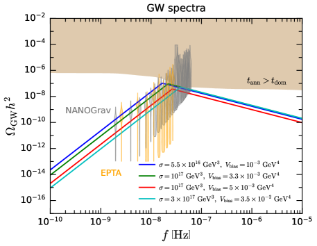
Figure 1: GW spectra generated by collapsing DWs for four sets of parameters. The gray and orange violins represent the reconstructed posterior distributions for the NANOGrav (gray violins) [2] and EPTA (orange violins) [4] observations of nHz GWs, respectively. The brown region is excluded by the requirement that DWs should annihilate before they dominate the universe.

In Fig. 1, we show the GW spectra generated by DWs for some benchmark parameters, compared with the reconstructed posterior distributions for the NANOGrav (gray violins) [2] and EPTA (orange violins) [4] signals. We find that the spectra with $\sigma\sim\mathcal{O}(10^{17})~{}\mathrm{GeV}^{3}$ and $V_{\mathrm{bias}}\sim\mathcal{O}(10^{-3})~{}\mathrm{GeV}^{4}$ can explain the PTA observations. As discussed above, DWs must annihilate before they dominate the energy of the universe. Thus, the time $t_{\mathrm{ann}}$ when DWs annihilate should be earlier than the time $t_{\mathrm{dom}}$ when DWs would dominate. According to Eqs. (18), (19) and (24), this gives upper limits on the GW spectra from collapsing DWs. In Fig. 1, the unavailable region corresponding to $t_{\mathrm{ann}}>t_{\mathrm{dom}}$ is shaded by the brown color.

III Freeze-in dark matter and the induced $Z_{2}$-violating potential

So far, the $Z_{2}$-violating potential is introduced by hand. In the following, we will consider it to be generated by loops of fermionic dark matter through a Yukawa interaction with the scalar field $S$. To be precise, we introduce a Dirac fermion field $\chi$, which is a singlet under all the SM gauge symmetries. The Lagrangian involving $\chi$ is

$$\mathcal{L}_{\chi}=\bar{\chi}(i\not{\partial}-m_{\chi})\chi+y_{\chi}S\bar{\chi}\chi,$$ (27)

where $y_{\chi}$ is the Yukawa coupling constant. When $S$ acquires a nonzero VEV, $\langle S\rangle\approx\pm v_{s}$, the mass of $\chi$ receives a correction, $m^{(\pm)}_{\chi}\approx m_{\chi}\mp y_{\chi}v_{s}$. In this work, we assume that $m_{\chi}\gg y_{\chi}v_{s}$, so $m^{(\pm)}_{\chi}\approx m_{\chi}$ holds.

After reheating, $s$ bosons are in thermal equilibrium with the SM particles due to the $|H|^{2}S^{2}$ interaction, while $\chi$ fermions are assumed to be out of equilibrium with nearly vanishing number density. This requires $y_{\chi}$ to be a feeble coupling constant. In this case, $\chi$ fermions could be produced via $s$ decays but never reach thermal equilibrium if $y_{\chi}$ is extremely small, say, $\sim\mathcal{O}(10^{-10})$. This is the well-known freeze-in mechanism of DM production [106], and $\chi$ acts as a DM candidate. The evolution of the DM number density $n_{\chi}$ is determined by the Boltzmann equation [127]

$$\frac{dn_{\chi}}{dt}+3Hn_{\chi}\approx\frac{m_{S}^{2}T}{\pi^{2}}\Gamma_{s\rightarrow\chi\bar{\chi}}\tilde{K}_{1}\left(x_{S},0,0,1,0,0\right),$$ (28)

where $x_{i}\equiv m_{i}/T$, and $\Gamma_{s\rightarrow\chi\bar{\chi}}$ is the $s\rightarrow\chi\bar{\chi}$ partial decay width given by

$$\Gamma_{s\rightarrow\chi\bar{\chi}}\approx\frac{y_{\chi}^{2}m_{s}}{8\pi}$$ (29)

for $m_{\chi}\ll m_{s}$. The function $\tilde{K}_{1}\left(x_{1},x_{2},x_{3},\eta_{1},\eta_{2},\eta_{3}\right)$ is defined as

$$\tilde{K}_{1}\left(x_{1},x_{2},x_{3},\eta_{1},\eta_{2},\eta_{3}\right)\equiv\frac{1}{(4\pi)^{2}p_{\mathrm{CM}}T}\int\prod_{i=1}^{3}\left(\frac{d^{3}p_{i}}{E_{i}}\frac{1}{e^{E_{i}/T}-\eta_{i}}\right)e^{E_{1}/T}\delta^{(4)}\left(p_{1}-p_{2}-p_{3}\right)$$ (30)

By solving Eq. (28), the $\chi$ number density at the present time $t_{0}$ can be approximated by [127]

$$n_{\chi}(t_{0})\approx\frac{3.434s_{0}M_{\mathrm{Pl}}\Gamma_{s\rightarrow\chi\bar{\chi}}}{[g_{\ast}(m_{s}/3)]^{3/2}m_{s}^{2}},$$ (31)

where $g_{\ast}(m_{s}/3)\approx 108$, $s_{0}$ is the present entropy density, and $M_{\mathrm{Pl}}\approx 2.4\times 10^{18}~{}\mathrm{GeV}$ is the reduced Planck mass. The $\chi$ relic density is then given by

$$\Omega_{\chi}h^{2}\approx 2.74\times 10^{8}~{}\frac{m_{\chi}}{\mathrm{GeV}}\frac{n_{\chi}(t_{0})}{s_{0}}\approx 8.13\times 10^{22}~{}\frac{y_{\chi}^{2}m_{\chi}}{m_{s}}.$$ (32)

On the other hand, the observed value of the DM relic density is $\Omega_{\mathrm{DM}}h^{2}=0.1200\pm 0.0012$ [128], which implies that the Yukawa coupling $y_{\chi}$ should be feeble.

In the potential (15), the $Z_{2}$-violating term is characterized by the parameter $\epsilon$, which is related to $\kappa_{1}$ and $\kappa_{3}$ via Eq. (16). Taking $\lambda_{S}\sim 0.2$, $\sigma\sim 10^{17}~{}\mathrm{GeV}^{3}$, and $V_{\mathrm{bias}}\sim 10^{-3}~{}\mathrm{GeV}^{4}$, which lead to a GW spectrum accounting for the recent PTA observations, we obtain $\epsilon\sim\mathcal{O}(10^{-26})$ from Eqs. (8) and (17). Note that the $S\bar{\chi}\chi$ Yukawa interaction explicitly breaks the $Z_{2}$ symmetry even if the tree-level $Z_{2}$-violating potential is absent. It is natural to conjecture that such an extremely tiny $\epsilon$ is originated from the feeble Yukawa interaction through $\chi$ loops.

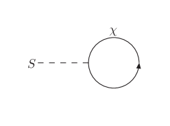
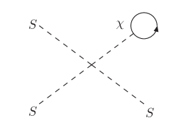
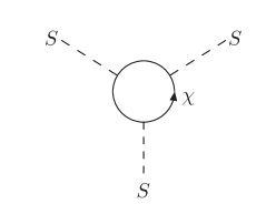
Figure 2: Examples of one-loop diagrams for generating the $Z_{2}$-violating potential terms.

In Fig. 2, we show some one-loop diagrams relevant to the generation of the $Z_{2}$-violating couplings $\kappa_{1}$ and $\kappa_{3}$. The first two diagrams contains the one-loop tadpole diagrams of $S$ and they give the dominant contributions to $\kappa_{1}$ and $\kappa_{3}$. Although the third diagram also contributes to $\kappa_{3}$, it is negligible compared with the second diagram due to a $y_{\chi}^{3}$ suppression. Our further calculation leads to the $\epsilon$ value at the $m_{s}$ scale as

$$\epsilon(m_{s})\approx\frac{3\lambda_{S}^{3/2}y_{\chi}}{\sqrt{2}\pi^{2}}\left(\frac{m_{\chi}}{m_{s}}\right)^{3}\ln\frac{\Lambda_{\mathrm{UV}}}{m_{s}},$$ (33)

where $\epsilon=0$ at some ultraviolet (UV) scale $\Lambda_{\mathrm{UV}}$ is assumed. Below we assume $\Lambda_{\mathrm{UV}}=M_{\mathrm{Pl}}$. Thus, $\lambda_{S}\sim 0.2$ and $v_{s}\sim 10^{5}~{}\mathrm{GeV}$ lead to $\epsilon(m_{s})\sim 0.6y_{\chi}(m_{\chi}/m_{s})^{3}$.

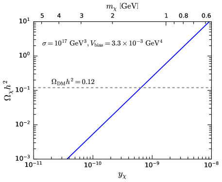
Figure 3: DM relic density as a function of the Yukawa coupling $y_{\chi}$ with fixed $\sigma=10^{17}~{}\mathrm{GeV}^{3}$, $V_{\mathrm{bias}}=3.3\times 10^{-3}~{}\mathrm{GeV}^{4}$, and $\lambda_{S}=0.2$. The upper horizontal axis denotes the value of $m_{\chi}$. The horizontal dashed line corresponds to the Planck observation value of the DM relic density [128].

By taking $\lambda_{S}=0.2$, $\sigma=10^{17}~{}\mathrm{GeV}^{3}$, and $V_{\mathrm{bias}}=3.3\times 10^{-3}~{}\mathrm{GeV}^{4}$, which correspond to the GW spectrum denoted by the green line in Fig. 1, we obtain $v_{s}=6.19\times 10^{5}~{}\mathrm{GeV}$, $m_{s}=3.91\times 10^{5}~{}\mathrm{GeV}$, $\epsilon=3.58\times 10^{-26}$, $T_{\mathrm{ann}}=163~{}\mathrm{MeV}$, $\Omega_{\mathrm{GW}}^{\mathrm{peak}}h^{2}=9.44\times 10^{-8}$, and $f_{\mathrm{peak}}=2.18\times 10^{-8}~{}\mathrm{Hz}$. Then, $y_{\chi}$ and $m_{\chi}$ are related by Eq. (33). For this set of parameters, the predicted DM relic density as a function of $y_{\chi}$ is shown in Fig. 3, with the upper horizontal axis corresponding to $m_{\chi}$. We find that both the extremely tiny $\epsilon\sim\mathcal{O}(10^{-26})$ and the observed DM relic density $\Omega_{\mathrm{DM}}h^{2}=0.12$ can be naturally explained by the feeble Yukawa coupling $y_{\chi}\sim\mathcal{O}(10^{-10})$. Therefore, our theory can simultaneously explain the recent PTA observations of nHz GWs and the DM relic via freeze-in production.

IV Favored parameter ranges

In this section, we investigate the parameter ranges favored by both the PTA GW observations and the observed DM relic density. Our model has four free parameters, which can be chosen to be $\lambda_{S}$, $y_{\chi}$, $m_{s}$, and $m_{\chi}$. In the following analysis, we fix the quartic coupling $\lambda_{S}=0.2$ to reduce one free parameter.

In Fig. 4, the GW spectra for four benchmark points with $m_{\chi}=1.1\text{--}2.5~{}\mathrm{GeV}$ and $m_{s}=(3.5\text{--}5)\times 10^{5}~{}\mathrm{GeV}$ are shown. For all these benchmark points, the Yukawa coupling $y_{\chi}$ is adjusted to give the mean value of the observed DM relic density $\Omega_{\chi}h^{2}=0.12$. We can see that the GW spectrum is quite sensitive to $m_{\chi}$ and $m_{s}$, limiting them varying within roughly one order of magnitude.

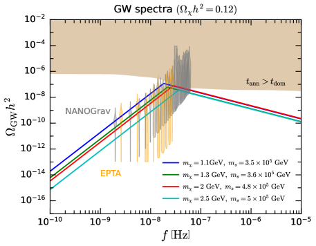
Figure 4: Same as in Fig. 1, but for GW spectra corresponding to different values of $m_{\chi}$ and $m_{s}$ with $\lambda_{S}=0.2$ fixed and $y_{\chi}$ adjusted to give $\Omega_{\chi}h^{2}=0.12$.

In our model, after the annihilation of DWs, most of their energy releases to the SM thermal bath. In this case, the NANOGrav collaboration has reconstructed the posterior distributions of $(T_{\mathrm{ann}},\alpha_{\ast})$ accounting for the observed nHz GW signal, as shown in the left panel of Fig. 12 in Ref. [2]. We use this result to study the favored parameter regions. In Fig. 5, the Yukawa coupling is fixed as $y_{\chi}=6.4\times 10^{-10}$, and the deep blue and light blue regions in the $m_{\chi}$-$m_{S}$ plane correspond to the 68% and 95% Bayesian credible regions favored by the NANOGrav data. It shows a high correlation between $m_{\chi}$ and $m_{S}$, which can be understood by the behavior of the GW peak amplitude, $\Omega_{\mathrm{GW}}^{\mathrm{peak}}h^{2}\propto m_{s}^{10}/m_{\chi}^{6}$, inferred from Eqs. (24) and (33).

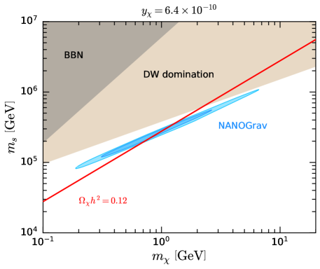
Figure 5: Parameter regions favored by the NANOGrav GW signal in the $m_{\chi}$-$m_{s}$ plane for $y_{\chi}=6.4\times 10^{-10}$. The deep blue and light blue regions corresponds to the 68% and 95% Bayesian credible regions favored by the NANOGrav data, respectively. The red line denotes the mean value of the Planck observation of the DM relic density, $\Omega_{\chi}h^{2}=0.12$. The brown and gray regions are excluded because DWs would dominate the universe and would inject energetic particles to affect BBN, respectively.

In Fig. 5, $\Omega_{\chi}h^{2}=0.12$ corresponds to a red line, which intersects the regions favored by the NANOGrav GW observation. Thus, both the PTA GW signal and the observed DM relic density can be well interpreted. Moreover, the brown and gray regions are excluded by the requirements that DWs should collapse before they dominate the universe and before the BBN epoch, respectively. We find that these constraints do not exclude the NANOGrav 95% Bayesian credible region.

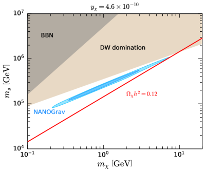
(a) $y_{\chi}=4.6\times 10^{-10}$.

(b) $y_{\chi}=8.7\times 10^{-10}$.

Figure 6: Same as in Fig. 5, but for $y_{\chi}=4.6\times 10^{-10}$ (a) and $y_{\chi}=8.7\times 10^{-10}$ (b).

The intersection of the $\Omega_{\chi}h^{2}=0.12$ line and the NANOGrav favored regions sensitively depends on the value of $y_{\chi}$. Our calculation shows that such a intersection can only happen for $4.6\times 10^{-10}\lesssim y_{\chi}\lesssim 8.7\times 10^{-10}$. In the left and right panels of Fig. 6, we demonstrate the results for $y_{\chi}=4.6\times 10^{-10}$ and $y_{\chi}=8.7\times 10^{-10}$, respectively. In both cases, the $\Omega_{\chi}h^{2}=0.12$ line can only touch the edge of the NANOGrav 95% Bayesian credible region. To sum up, for $\lambda_{S}=0.2$, we find that the preferred parameter ranges where our model can simultaneously explain the NANOGrav GW signal and the DM relic density are

$$4.6\times 10^{-10}\lesssim y_{\chi}\lesssim 8.7\times 10^{-10},$$ (34)

$$0.17~{}\mathrm{GeV}\lesssim m_{\chi}\lesssim 7.5~{}\mathrm{GeV},$$

$$8.1\times 10^{4}~{}\mathrm{GeV}\lesssim m_{s}\lesssim 10^{6}~{}\mathrm{GeV}.$$

V Summary

In this work, we studied the interplay between the SGWB from collapsing DWs and FIMP DM. The newly introduced real scalar field $S$ satisfies a $Z_{2}$ symmetry in the tree-level potential, which, however, is violated by the Yukawa coupling $y_{\chi}$ with a fermion field $\chi$. The linear and cubic terms of $S$ can be induced by the Yukawa coupling at one-loop level, and they explicitly break the $Z_{2}$ symmetry of the potential, leading to an energy bias between the two minima. Thus, after the spontaneous breaking of the $Z_{2}$ symmetry, unstable DWs would be formed. We considered that the Yukawa coupling is feeble, i.e., $y_{\chi}\sim\mathcal{O}(10^{-10})$, and the $\chi$ fermions become FIMPs that are produced by the freeze-in mechanism, accounting for dark matter in the universe.

On the other hand, four PTA collaborations have recently reported evidences of a SGWB at nHz frequencies, which could be produced by the collapse of DWs in the early universe. Since the tiny $Z_{2}$-violating potential induced by the feeble Yukawa coupling leads to unstable DWs, it is possible that our model can explain the PTA data. Comparing with the posterior distributions in the GW spectrum reconstructed by the NANOGrav and EPTA data, our analysis showed that the $Z_{2}$-violating coefficient should be as tiny as $\epsilon\sim 10^{-26}$, which can be naturally induced by the feeble Yukawa couplings $y_{\chi}\sim\mathcal{O}(10^{-10})$ at one-loop level. Thus, our scenario is very suitable for interpreting the PTA observations of the nHz SGWB.

Moreover, we investigated the parameter regions where both the PTA GW observations and the DM relic density can be simultaneously explained. We found that the parameters should satisfy $y_{\chi}\in(4.6\times 10^{-10},8.7\times 10^{-10})$, $m_{\chi}\in(0.17,7.5)~{}\mathrm{GeV}$, and $m_{s}\in(8.1\times 10^{4},10^{6})~{}\mathrm{GeV}$ for a fixed quartic scalar couplings $\lambda_{S}=0.2$. The corresponding regions also fulfill the requirements that DWs should collapse before they overclose the universe and they should not affect the BBN.

- [1] NANOGrav Collaboration, G. Agazie et al., “The NANOGrav 15 yr Data Set: Evidence for a Gravitational-wave Background,” Astrophys. J. Lett. 951 (2023) L8, arXiv:2306.16213 [astro-ph.HE].
- [2] NANOGrav Collaboration, A. Afzal et al., “The NANOGrav 15 yr Data Set: Search for Signals from New Physics,” Astrophys. J. Lett. 951 (2023) L11, arXiv:2306.16219 [astro-ph.HE].
- [3] J. Antoniadis et al., “The second data release from the European Pulsar Timing Array III. Search for gravitational wave signals,” arXiv:2306.16214 [astro-ph.HE].
- [4] J. Antoniadis et al., “The second data release from the European Pulsar Timing Array: V. Implications for massive black holes, dark matter and the early Universe,” arXiv:2306.16227 [astro-ph.CO].
- [5] H. Xu et al., “Searching for the Nano-Hertz Stochastic Gravitational Wave Background with the Chinese Pulsar Timing Array Data Release I,” Res. Astron. Astrophys. 23 (2023) 075024, arXiv:2306.16216 [astro-ph.HE].
- [6] D. J. Reardon et al., “Search for an Isotropic Gravitational-wave Background with the Parkes Pulsar Timing Array,” Astrophys. J. Lett. 951 (2023) L6, arXiv:2306.16215 [astro-ph.HE].
- [7] J. Ellis, M. Fairbairn, G. Hütsi, J. Raidal, J. Urrutia, V. Vaskonen, and H. Veermäe, “Gravitational Waves from SMBH Binaries in Light of the NANOGrav 15-Year Data,” arXiv:2306.17021 [astro-ph.CO].
- [8] Z.-Q. Shen, G.-W. Yuan, Y.-Y. Wang, and Y.-Z. Wang, “Dark Matter Spike surrounding Supermassive Black Holes Binary and the nanohertz Stochastic Gravitational Wave Background,” arXiv:2306.17143 [astro-ph.HE].
- [9] A. Ghoshal and A. Strumia, “Probing the Dark Matter density with gravitational waves from super-massive binary black holes,” arXiv:2306.17158 [astro-ph.CO].
- [10] H.-L. Huang, Y. Cai, J.-Q. Jiang, J. Zhang, and Y.-S. Piao, “Supermassive primordial black holes in multiverse: for nano-Hertz gravitational wave and high-redshift JWST galaxies,” arXiv:2306.17577 [gr-qc].
- [11] T. Broadhurst, C. Chen, T. Liu, and K.-F. Zheng, “Binary Supermassive Black Holes Orbiting Dark Matter Solitons: From the Dual AGN in UGC4211 to NanoHertz Gravitational Waves,” arXiv:2306.17821 [astro-ph.HE].
- [12] P. F. Depta, K. Schmidt-Hoberg, and C. Tasillo, “Do pulsar timing arrays observe merging primordial black holes?,” arXiv:2306.17836 [astro-ph.CO].
- [13] Y.-C. Bi, Y.-M. Wu, Z.-C. Chen, and Q.-G. Huang, “Implications for the Supermassive Black Hole Binaries from the NANOGrav 15-year Data Set,” arXiv:2307.00722 [astro-ph.CO].
- [14] J. R. Westernacher-Schneider, J. Zrake, A. MacFadyen, and Z. Haiman, “Characteristic signatures of accreting binary black holes produced by eccentric minidisks,” arXiv:2307.01154 [astro-ph.HE].
- [15] Y. Gouttenoire, S. Trifinopoulos, G. Valogiannis, and M. Vanvlasselaer, “Scrutinizing the Primordial Black Holes Interpretation of PTA Gravitational Waves and JWST Early Galaxies,” arXiv:2307.01457 [astro-ph.CO].
- [16] L. Bian, S. Ge, J. Shu, B. Wang, X.-Y. Yang, and J. Zong, “Gravitational wave sources for Pulsar Timing Arrays,” arXiv:2307.02376 [astro-ph.HE].
- [17] A. Ashoorioon, K. Rezazadeh, and A. Rostami, “NANOGrav signal from the end of inflation and the LIGO mass and heavier primordial black holes,” Phys. Lett. B 835 (2022) 137542, arXiv:2202.01131 [astro-ph.CO].
- [18] E. Madge, E. Morgante, C. Puchades-Ibáñez, N. Ramberg, W. Ratzinger, S. Schenk, and P. Schwaller, “Primordial gravitational waves in the nano-Hertz regime and PTA data – towards solving the GW inverse problem,” arXiv:2306.14856 [hep-ph].
- [19] C. Han, K.-P. Xie, J. M. Yang, and M. Zhang, “Self-interacting dark matter implied by nano-Hertz gravitational waves,” arXiv:2306.16966 [hep-ph].
- [20] E. Megias, G. Nardini, and M. Quiros, “Pulsar Timing Array Stochastic Background from light Kaluza-Klein resonances,” arXiv:2306.17071 [hep-ph].
- [21] K. Fujikura, S. Girmohanta, Y. Nakai, and M. Suzuki, “NANOGrav Signal from a Dark Conformal Phase Transition,” arXiv:2306.17086 [hep-ph].
- [22] A. Addazi, Y.-F. Cai, A. Marciano, and L. Visinelli, “Have pulsar timing array methods detected a cosmological phase transition?,” arXiv:2306.17205 [astro-ph.CO].
- [23] P. Athron, A. Fowlie, C.-T. Lu, L. Morris, L. Wu, Y. Wu, and Z. Xu, “Can Supercooled Phase Transitions explain the Gravitational Wave Background observed by Pulsar Timing Arrays?,” arXiv:2306.17239 [hep-ph].
- [24] S. Jiang, A. Yang, J. Ma, and F. P. Huang, “Implication of nano-Hertz stochastic gravitational wave on dynamical dark matter through a first-order phase transition,” arXiv:2306.17827 [hep-ph].
- [25] Y. Xiao, J. M. Yang, and Y. Zhang, “Implications of Nano-Hertz Gravitational Waves on Electroweak Phase Transition in the Singlet Dark Matter Model,” arXiv:2307.01072 [hep-ph].
- [26] S.-P. Li and K.-P. Xie, “Collider test of nano-Hertz gravitational waves from pulsar timing arrays,” Phys. Rev. D 108 (2023) 055018, arXiv:2307.01086 [hep-ph].
- [27] T. Ghosh, A. Ghoshal, H.-K. Guo, F. Hajkarim, S. F. King, K. Sinha, X. Wang, and G. White, “Did we hear the sound of the Universe boiling? Analysis using the full fluid velocity profiles and NANOGrav 15-year data,” arXiv:2307.02259 [astro-ph.HE].
- [28] P. Athron, C. Balázs, T. E. Gonzalo, and M. Pearce, “Falsifying Pati-Salam models with LIGO,” arXiv:2307.02544 [hep-ph].
- [29] J. S. Cruz, F. Niedermann, and M. S. Sloth, “NANOGrav meets Hot New Early Dark Energy and the origin of neutrino mass,” arXiv:2307.03091 [astro-ph.CO].
- [30] Y.-M. Wu, Z.-C. Chen, and Q.-G. Huang, “Cosmological Interpretation for the Stochastic Signal in Pulsar Timing Arrays,” arXiv:2307.03141 [astro-ph.CO].
- [31] P. Di Bari and M. H. Rahat, “The split majoron model confronts the NANOGrav signal,” arXiv:2307.03184 [hep-ph].
- [32] Y. Gouttenoire, “First-order Phase Transition interpretation of PTA signal produces solar-mass Black Holes,” arXiv:2307.04239 [hep-ph].
- [33] A. Salvio, “Supercooling in Radiative Symmetry Breaking: Theory Extensions, Gravitational Wave Detection and Primordial Black Holes,” arXiv:2307.04694 [hep-ph].
- [34] M. Ahmadvand, L. Bian, and S. Shakeri, “A Heavy QCD Axion model in Light of Pulsar Timing Arrays,” arXiv:2307.12385 [hep-ph].
- [35] J. Ellis and M. Lewicki, “Cosmic String Interpretation of NANOGrav Pulsar Timing Data,” Phys. Rev. Lett. 126 (2021) 041304, arXiv:2009.06555 [astro-ph.CO].
- [36] Z.-Y. Qiu and Z.-H. Yu, “Gravitational waves from cosmic strings associated with pseudo-Nambu-Goldstone dark matter*,” Chin. Phys. C 47 (2023) 085104, arXiv:2304.02506 [hep-ph].
- [37] J. Ellis, M. Lewicki, C. Lin, and V. Vaskonen, “Cosmic Superstrings Revisited in Light of NANOGrav 15-Year Data,” arXiv:2306.17147 [astro-ph.CO].
- [38] Z. Wang, L. Lei, H. Jiao, L. Feng, and Y.-Z. Fan, “The nanohertz stochastic gravitational-wave background from cosmic string Loops and the abundant high redshift massive galaxies,” arXiv:2306.17150 [astro-ph.HE].
- [39] N. Kitajima and K. Nakayama, “Nanohertz gravitational waves from cosmic strings and dark photon dark matter,” arXiv:2306.17390 [hep-ph].
- [40] A. Eichhorn, R. R. Lino dos Santos, and J. a. L. Miqueleto, “From quantum gravity to gravitational waves through cosmic strings,” arXiv:2306.17718 [gr-qc].
- [41] G. Lazarides, R. Maji, and Q. Shafi, “Superheavy quasi-stable strings and walls bounded by strings in the light of NANOGrav 15 year data,” arXiv:2306.17788 [hep-ph].
- [42] G. Servant and P. Simakachorn, “Constraining Post-Inflationary Axions with Pulsar Timing Arrays,” arXiv:2307.03121 [hep-ph].
- [43] S. Antusch, K. Hinze, S. Saad, and J. Steiner, “Singling out SO(10) GUT models using recent PTA results,” arXiv:2307.04595 [hep-ph].
- [44] W. Buchmuller, V. Domcke, and K. Schmitz, “Metastable cosmic strings,” arXiv:2307.04691 [hep-ph].
- [45] M. Yamada and K. Yonekura, “Dark baryon from pure Yang-Mills theory and its GW signature from cosmic strings,” arXiv:2307.06586 [hep-ph].
- [46] C.-W. Chiang and B.-Q. Lu, “Testing clockwork axion with gravitational waves,” JCAP 05 (2021) 049, arXiv:2012.14071 [hep-ph].
- [47] A. S. Sakharov, Y. N. Eroshenko, and S. G. Rubin, “Looking at the NANOGrav signal through the anthropic window of axionlike particles,” Phys. Rev. D 104 (2021) 043005, arXiv:2104.08750 [hep-ph].
- [48] S. F. King, D. Marfatia, and M. H. Rahat, “Towards distinguishing Dirac from Majorana neutrino mass with gravitational waves,” arXiv:2306.05389 [hep-ph].
- [49] S.-Y. Guo, M. Khlopov, X. Liu, L. Wu, Y. Wu, and B. Zhu, “Footprints of Axion-Like Particle in Pulsar Timing Array Data and JWST Observations,” arXiv:2306.17022 [hep-ph].
- [50] N. Kitajima, J. Lee, K. Murai, F. Takahashi, and W. Yin, “Nanohertz Gravitational Waves from Axion Domain Walls Coupled to QCD,” arXiv:2306.17146 [hep-ph].
- [51] Y. Bai, T.-K. Chen, and M. Korwar, “QCD-Collapsed Domain Walls: QCD Phase Transition and Gravitational Wave Spectroscopy,” arXiv:2306.17160 [hep-ph].
- [52] S. Blasi, A. Mariotti, A. Rase, and A. Sevrin, “Axionic domain walls at Pulsar Timing Arrays: QCD bias and particle friction,” arXiv:2306.17830 [hep-ph].
- [53] Y. Gouttenoire and E. Vitagliano, “Domain wall interpretation of the PTA signal confronting black hole overproduction,” arXiv:2306.17841 [gr-qc].
- [54] B. Barman, D. Borah, S. Jyoti Das, and I. Saha, “Scale of Dirac leptogenesis and left-right symmetry in the light of recent PTA results,” arXiv:2307.00656 [hep-ph].
- [55] B.-Q. Lu and C.-W. Chiang, “Nano-Hertz stochastic gravitational wave background from domain wall annihilation,” arXiv:2307.00746 [hep-ph].
- [56] X. K. Du, M. X. Huang, F. Wang, and Y. K. Zhang, “Did the nHZ Gravitational Waves Signatures Observed By NANOGrav Indicate Multiple Sector SUSY Breaking?,” arXiv:2307.02938 [hep-ph].
- [57] X.-F. Li, “Probing the high temperature symmetry breaking with gravitational waves from domain walls,” arXiv:2307.03163 [hep-ph].
- [58] E. Babichev, D. Gorbunov, S. Ramazanov, R. Samanta, and A. Vikman, “NANOGrav spectral index from melting domain walls,” arXiv:2307.04582 [hep-ph].
- [59] G. B. Gelmini and J. Hyman, “Catastrogenesis with unstable ALPs as the origin of the NANOGrav 15 yr gravitational wave signal,” arXiv:2307.07665 [hep-ph].
- [60] S. Ge, “Stochastic gravitational wave background: birth from axionic string-wall death,” arXiv:2307.08185 [gr-qc].
- [61] S. Vagnozzi, “Inflationary interpretation of the stochastic gravitational wave background signal detected by pulsar timing array experiments,” arXiv:2306.16912 [astro-ph.CO].
- [62] D. Borah, S. Jyoti Das, and R. Samanta, “Inflationary origin of gravitational waves with Miracle-less WIMP dark matter in the light of recent PTA results,” arXiv:2307.00537 [hep-ph].
- [63] K. Murai and W. Yin, “A Novel Probe of Supersymmetry in Light of Nanohertz Gravitational Waves,” arXiv:2307.00628 [hep-ph].
- [64] S. Datta, “Inflationary gravitational waves, pulsar timing data and low-scale-leptogenesis,” arXiv:2307.00646 [hep-ph].
- [65] D. Chowdhury, G. Tasinato, and I. Zavala, “Dark energy, D-branes, and Pulsar Timing Arrays,” arXiv:2307.01188 [hep-th].
- [66] X. Niu and M. H. Rahat, “NANOGrav signal from axion inflation,” arXiv:2307.01192 [hep-ph].
- [67] C. Unal, A. Papageorgiou, and I. Obata, “Axion-Gauge Dynamics During Inflation as the Origin of Pulsar Timing Array Signals and Primordial Black Holes,” arXiv:2307.02322 [astro-ph.CO].
- [68] H. Firouzjahi and A. Talebian, “Induced Gravitational Waves from Ultra Slow-Roll Inflation and Pulsar Timing Arrays Observations,” arXiv:2307.03164 [gr-qc].
- [69] S. Choudhury, “Single field inflation in the light of NANOGrav 15-year Data: Quintessential interpretation of blue tilted tensor spectrum through Non-Bunch Davies initial condition,” arXiv:2307.03249 [astro-ph.CO].
- [70] S. A. Hosseini Mansoori, F. Felegray, A. Talebian, and M. Sami, “PBHs and GWs from -inflation and NANOGrav 15-year data,” arXiv:2307.06757 [astro-ph.CO].
- [71] K. Cheung, C. J. Ouseph, and P.-Y. Tseng, “NANOGrav Signal and PBH from the Modified Higgs Inflation,” arXiv:2307.08046 [hep-ph].
- [72] Y.-F. Cai, X.-C. He, X. Ma, S.-F. Yan, and G.-W. Yuan, “Limits on scalar-induced gravitational waves from the stochastic background by pulsar timing array observations,” arXiv:2306.17822 [gr-qc].
- [73] S. Wang, Z.-C. Zhao, J.-P. Li, and Q.-H. Zhu, “Exploring the Implications of 2023 Pulsar Timing Array Datasets for Scalar-Induced Gravitational Waves and Primordial Black Holes,” arXiv:2307.00572 [astro-ph.CO].
- [74] L. Liu, Z.-C. Chen, and Q.-G. Huang, “Implications for the non-Gaussianity of curvature perturbation from pulsar timing arrays,” arXiv:2307.01102 [astro-ph.CO].
- [75] D. G. Figueroa, M. Pieroni, A. Ricciardone, and P. Simakachorn, “Cosmological Background Interpretation of Pulsar Timing Array Data,” arXiv:2307.02399 [astro-ph.CO].
- [76] Z. Yi, Q. Gao, Y. Gong, Y. Wang, and F. Zhang, “The waveform of the scalar induced gravitational waves in light of Pulsar Timing Array data,” arXiv:2307.02467 [gr-qc].
- [77] Q.-H. Zhu, Z.-C. Zhao, and S. Wang, “Joint implications of BBN, CMB, and PTA Datasets for Scalar-Induced Gravitational Waves of Second and Third orders,” arXiv:2307.03095 [astro-ph.CO].
- [78] Z.-Q. You, Z. Yi, and Y. Wu, “Constraints on primordial curvature power spectrum with pulsar timing arrays,” arXiv:2307.04419 [gr-qc].
- [79] S. Balaji, G. Domènech, and G. Franciolini, “Scalar-induced gravitational wave interpretation of PTA data: the role of scalar fluctuation propagation speed,” arXiv:2307.08552 [gr-qc].
- [80] G. Lambiase, L. Mastrototaro, and L. Visinelli, “Astrophysical neutrino oscillations after pulsar timing array analyses,” arXiv:2306.16977 [astro-ph.HE].
- [81] J. Yang, N. Xie, and F. P. Huang, “Nano-Hertz stochastic gravitational wave background as hints of ultralight axion particles,” arXiv:2306.17113 [hep-ph].
- [82] H. Deng, B. Bécsy, X. Siemens, N. J. Cornish, and D. R. Madison, “Searching for gravitational wave burst in PTA data with piecewise linear functions,” arXiv:2306.17130 [gr-qc].
- [83] G. Franciolini, D. Racco, and F. Rompineve, “Footprints of the QCD Crossover on Cosmological Gravitational Waves at Pulsar Timing Arrays,” arXiv:2306.17136 [astro-ph.CO].
- [84] G. Franciolini, A. Iovino, Junior., V. Vaskonen, and H. Veermae, “The recent gravitational wave observation by pulsar timing arrays and primordial black holes: the importance of non-gaussianities,” arXiv:2306.17149 [astro-ph.CO].
- [85] V. K. Oikonomou, “Flat Energy Spectrum of Primordial Gravitational Waves vs Peaks and the NANOGrav 2023 Observation,” arXiv:2306.17351 [astro-ph.CO].
- [86] K. Inomata, K. Kohri, and T. Terada, “The Detected Stochastic Gravitational Waves and Sub-Solar Primordial Black Holes,” arXiv:2306.17834 [astro-ph.CO].
- [87] C. Zhang, N. Dai, Q. Gao, Y. Gong, T. Jiang, and X. Lu, “Detecting new fundamental fields with Pulsar Timing Arrays,” arXiv:2307.01093 [gr-qc].
- [88] L. A. Anchordoqui, I. Antoniadis, and D. Lust, “Fuzzy Dark Matter, the Dark Dimension, and the Pulsar Timing Array Signal,” arXiv:2307.01100 [hep-ph].
- [89] R. A. Konoplya and A. Zhidenko, “Asymptotic tails of massive gravitons in light of pulsar timing array observations,” arXiv:2307.01110 [gr-qc].
- [90] R. Ebadi, S. Kumar, A. McCune, H. Tai, and L.-T. Wang, “Gravitational Waves from Stochastic Scalar Fluctuations,” arXiv:2307.01248 [astro-ph.CO].
- [91] K. T. Abe and Y. Tada, “Translating nano-Hertz gravitational wave background into primordial perturbations taking account of the cosmological QCD phase transition,” arXiv:2307.01653 [astro-ph.CO].
- [92] P. Bari, N. Bartolo, G. Domènech, and S. Matarrese, “Gravitational waves induced by scalar-tensor mixing,” arXiv:2307.05404 [astro-ph.CO].
- [93] G. Ye and A. Silvestri, “Can gravitational wave background feel wiggles in spacetime?,” arXiv:2307.05455 [astro-ph.CO].
- [94] S. Basilakos, D. V. Nanopoulos, T. Papanikolaou, E. N. Saridakis, and C. Tzerefos, “Signatures of Superstring theory in NANOGrav,” arXiv:2307.08601 [hep-th].
- [95] J.-H. Jin, Z.-C. Chen, Z. Yi, Z.-Q. You, L. Liu, and Y. Wu, “Confronting sound speed resonance with pulsar timing arrays,” arXiv:2307.08687 [astro-ph.CO].
- [96] M. Bousder, A. Riadsolh, A. E. Fatimy, M. E. Belkacemi, and H. Ez-Zahraouy, “Implications of the NANOGrav results for primordial black holes and Hubble tension,” arXiv:2307.10940 [gr-qc].
- [97] T. W. B. Kibble, “Topology of Cosmic Domains and Strings,” J. Phys. A 9 (1976) 1387–1398.
- [98] Y. B. Zeldovich, I. Y. Kobzarev, and L. B. Okun, “Cosmological Consequences of the Spontaneous Breakdown of Discrete Symmetry,” Zh. Eksp. Teor. Fiz. 67 (1974) 3–11.
- [99] A. Vilenkin, “Gravitational Field of Vacuum Domain Walls and Strings,” Phys. Rev. D 23 (1981) 852–857.
- [100] G. B. Gelmini, M. Gleiser, and E. W. Kolb, “Cosmology of Biased Discrete Symmetry Breaking,” Phys. Rev. D 39 (1989) 1558.
- [101] S. E. Larsson, S. Sarkar, and P. L. White, “Evading the cosmological domain wall problem,” Phys. Rev. D 55 (1997) 5129–5135, arXiv:hep-ph/9608319.
- [102] J. Preskill, S. P. Trivedi, F. Wilczek, and M. B. Wise, “Cosmology and broken discrete symmetry,” Nucl. Phys. B 363 (1991) 207–220.
- [103] M. Gleiser and R. Roberts, “Gravitational waves from collapsing vacuum domains,” Phys. Rev. Lett. 81 (1998) 5497–5500, arXiv:astro-ph/9807260.
- [104] T. Hiramatsu, M. Kawasaki, and K. Saikawa, “Gravitational Waves from Collapsing Domain Walls,” JCAP 05 (2010) 032, arXiv:1002.1555 [astro-ph.CO].
- [105] M. Kawasaki and K. Saikawa, “Study of gravitational radiation from cosmic domain walls,” JCAP 09 (2011) 008, arXiv:1102.5628 [astro-ph.CO].
- [106] L. J. Hall, K. Jedamzik, J. March-Russell, and S. M. West, “Freeze-In Production of FIMP Dark Matter,” JHEP 03 (2010) 080, arXiv:0911.1120 [hep-ph].
- [107] N. Bernal, M. Heikinheimo, T. Tenkanen, K. Tuominen, and V. Vaskonen, “The Dawn of FIMP Dark Matter: A Review of Models and Constraints,” Int. J. Mod. Phys. A 32 (2017) 1730023, arXiv:1706.07442 [hep-ph].
- [108] T. Hambye, M. H. G. Tytgat, J. Vandecasteele, and L. Vanderheyden, “Dark matter direct detection is testing freeze-in,” Phys. Rev. D 98 (2018) 075017, arXiv:1807.05022 [hep-ph].
- [109] L. Bian and Y.-L. Tang, “Thermally modified sterile neutrino portal dark matter and gravitational waves from phase transition: The Freeze-in case,” JHEP 12 (2018) 006, arXiv:1810.03172 [hep-ph].
- [110] G. Bélanger et al., “LHC-friendly minimal freeze-in models,” JHEP 02 (2019) 186, arXiv:1811.05478 [hep-ph].
- [111] J. M. No, P. Tunney, and B. Zaldivar, “Probing Dark Matter freeze-in with long-lived particle signatures: MATHUSLA, HL-LHC and FCC-hh,” JHEP 03 (2020) 022, arXiv:1908.11387 [hep-ph].
- [112] G. Brooijmans et al., “Les Houches 2019 Physics at TeV Colliders: New Physics Working Group Report,” in 11th Les Houches Workshop on Physics at TeV Colliders: PhysTeV Les Houches. 2, 2020, arXiv:2002.12220 [hep-ph].
- [113] C. Dvorkin, T. Lin, and K. Schutz, “Cosmology of Sub-MeV Dark Matter Freeze-In,” Phys. Rev. Lett. 127 (2021) 111301, arXiv:2011.08186 [astro-ph.CO].
- [114] L. Calibbi, F. D’Eramo, S. Junius, L. Lopez-Honorez, and A. Mariotti, “Displaced new physics at colliders and the early universe before its first second,” JHEP 05 (2021) 234, arXiv:2102.06221 [hep-ph].
- [115] L. Bian, Y.-L. Tang, and R. Zhou, “FIMP dark matter mediated by a massive gauge boson around the phase transition period and the gravitational waves production,” Phys. Rev. D 106 (2022) 035028, arXiv:2111.10608 [hep-ph].
- [116] G. Elor, R. McGehee, and A. Pierce, “Maximizing Direct Detection with Highly Interactive Particle Relic Dark Matter,” Phys. Rev. Lett. 130 (2023) 031803, arXiv:2112.03920 [hep-ph].
- [117] D. K. Ghosh, S. Jeesun, and D. Nanda, “Long-lived inert Higgs boson in a fast expanding universe and its imprint on the cosmic microwave background,” Phys. Rev. D 106 (2022) 115001, arXiv:2206.04940 [hep-ph].
- [118] P. N. Bhattiprolu, G. Elor, R. McGehee, and A. Pierce, “Freezing-in hadrophilic dark matter at low reheating temperatures,” JHEP 01 (2023) 128, arXiv:2210.15653 [hep-ph].
- [119] X.-M. Jiang, C. Cai, Y.-H. Su, and H.-H. Zhang, “Freeze-in Production of Pseudo-Nambu-Goldstone Dark Matter Model with a Real Scalar,” arXiv:2302.02418 [hep-ph].
- [120] S. Ramazanov, E. Babichev, D. Gorbunov, and A. Vikman, “Beyond freeze-in: Dark matter via inverse phase transition and gravitational wave signal,” Phys. Rev. D 105 (2022) 063530, arXiv:2104.13722 [hep-ph].
- [121] E. Babichev, D. Gorbunov, S. Ramazanov, and A. Vikman, “Gravitational shine of dark domain walls,” JCAP 04 (2022) 028, arXiv:2112.12608 [hep-ph].
- [122] K. Nakayama, F. Takahashi, and N. Yokozaki, “Gravitational waves from domain walls and their implications,” Phys. Lett. B 770 (2017) 500–506, arXiv:1612.08327 [hep-ph].
- [123] K. Saikawa, “A review of gravitational waves from cosmic domain walls,” Universe 3 (2017) 40, arXiv:1703.02576 [hep-ph].
- [124] T. Hiramatsu, M. Kawasaki, and K. Saikawa, “On the estimation of gravitational wave spectrum from cosmic domain walls,” JCAP 02 (2014) 031, arXiv:1309.5001 [astro-ph.CO].
- [125] L. Husdal, “On Effective Degrees of Freedom in the Early Universe,” Galaxies 4 (2016) 78, arXiv:1609.04979 [astro-ph.CO].
- [126] C. Caprini, R. Durrer, T. Konstandin, and G. Servant, “General Properties of the Gravitational Wave Spectrum from Phase Transitions,” Phys. Rev. D 79 (2009) 083519, arXiv:0901.1661 [astro-ph.CO].
- [127] G. Bélanger, F. Boudjema, A. Goudelis, A. Pukhov, and B. Zaldivar, “micrOMEGAs5.0 : Freeze-in,” Comput. Phys. Commun. 231 (2018) 173–186, arXiv:1801.03509 [hep-ph].
- [128] Planck Collaboration, N. Aghanim et al., “Planck 2018 results. VI. Cosmological parameters,” Astron. Astrophys. 641 (2020) A6, arXiv:1807.06209 [astro-ph.CO]. [Erratum: Astron.Astrophys. 652, C4 (2021)].