Improve Long-term Memory Learning Through Rescaling the Error Temporally

Abstract

This paper studies the error metric selection for long-term memory learning in sequence modelling. We examine the bias towards short-term memory in commonly used errors, including mean absolute/squared error. Our findings show that all temporally positive-weighted errors are biased towards short-term memory in learning linear functionals. To reduce this bias and improve long-term memory learning, we propose the use of a temporally rescaled error. In addition to reducing the bias towards short-term memory, this approach can also alleviate the vanishing gradient issue. We conduct numerical experiments on different long-memory tasks and sequence models to validate our claims. Numerical results confirm the importance of appropriate temporally rescaled error for effective long-term memory learning. To the best of our knowledge, this is the first work that quantitatively analyzes different errors’ memory bias towards short-term memory in sequence modelling.

1 Introduction

The challenge of comprehending long-term relationships is a perennial issue within the realm of sequence modeling. Sequences that manifest these characteristics are often classified as having a long “memory”. The acquisition of knowledge pertaining to this prolonged memory is pivotal for various applications, notably in the field of time series prediction [1], machine translation [2], speech recognition [3], language modelling [4], reinforcement learning [5]. To further improve the performance on these tasks, designing more scalable models [6] and finding better optimization methods [7] are two common directions.

Numerous models aimed at enhancing the retention of long-term memory in sequential data. Recurrent-type neural networks such as RNN [8], GRU [6] and LSTM [9] are popular models for learning sequential relationship. However, recurrent models can suffer from the vanishing gradient issue and they have an exponentially decaying memory [10, 11, 12]. The ReLU activation was initially introduced to tackle the vanishing gradient problem prevalent in sequence modelling, as noted by Pascanu et al. [10]. More recently, innovative structures for sequence modeling have emerged, such as Temporal Convolution Networks (TCN) [13] and attention-based models [14]. These are attempts from the model construction perspective.

Apart from the model design aspect, various parameterization techniques have been explored. Models like AntisymmetricRNN [15], UnitaryRNN [16], IndRNN [17], KRU[18], ExpRNN [19], LEM[20], CoRNN [21], Hippo [22, 23] all can be regarded as the approach to seek better parameterization methods. While these models differ from the original recurrent networks, they do not expand the approximation space. Consequently, the advantages they offer in terms of speed and stability primarily stem from an optimization standpoint. Besides the recurrent neural networks, Romero et al. [24] also proposes implicit parameterization for convolutional kernels which facilitate the learning of long memory.

In this paper, we investigate the feasibility of learning long-term memory based on the error metric selection. We emphasize this approach is orthogonal to the previous approaches including model construction and parameterization selection. We evaluate the bias of error towards short-term memory. It is proved that commonly-used error such as mean absolute/squared error are biased towards short-term memory.

To summarize, our main contibutions are

1. We identify the existence of bias towards short-term memory among mean absolute/squared error. In particular, we quantify the scale of memory bias in the linear functional case.

2. We extend the memory bias analysis to more general temporally positive-weighted errors.

3. We confirm the theoretical claims based on numerical experiments on linear functional learning, copying problem and text summarization task. The effectiveness of rescaling error temporally are justified via different sequence models.

Paper structure

In Section 2, we give the setup of the sequence modelling and the definition of memory function for general sequence to sequence relationship. In Section 3, we present the main results on the memory bias of MSE/MAE and general temporally positive-weighted errors. A subfamily of temporally positive-weighted errors are selected to compare the memory bias effects. In Section 4, the numerical experiments are shown to validate the claims in Section 3. The related works from sequence modelling are summarized in Section 5.

2 Problem formulation

We start with the setup of the sequence modelling. Next we summarize different memory definitions in sequence modelling. The memory evaluation method is important for the fair comparison of the memory bias.

2.1 Sequence modelling

In sequence modelling, a map $\{H_{t}\}_{t\in\mathbb{R}}$ is learned between input sequence $\mathbf{x}=\{x_{t}\}$ and the corresponding output sequence $\mathbf{y}=\{y_{t}\}$. This mapping can be regarded as sequence of functionals from the mathematical perspective.

$$y_{t}=H_{t}(\mathbf{x}).$$ (1)

Notice here $t$ is not limited to discrete index. For theoretical study perspective, it’s common to assume the index $t\in\mathbb{R}$ to be unbounded. In this paper, when we consider the specific memory bias, we will focus on a fixed time horizon $t\in[0,T],T>0$. We make the additional assumption that the target sequential relationship is time-homogeneous. This characteristic is crucial for ensuring the effectiveness of a model when trained at one time interval and evaluated at a different time interval.

2.2 Memory evaluation in sequence modelling

Now we summarize different memory function definitions commonly used in sequence modelling and give the memory function definition used in our paper.

Finite horizon memory function

Given sequences $\{x_{t}\}$ and $\{y_{t}\}$. Assume there exists a positive horizon $\tau$ such that the output $y_{t}$ is only a deterministic function of inputs $x_{t-\tau},x_{t-\tau+1},\dots,x_{t-1},x_{t}$.

$$y_{t}=f(x_{t-\tau},x_{t-\tau+1},\dots,x_{t-1},x_{t}).$$ (2)

If there is no such positive horizon, it is said to have a memory with infinite horizon.

Representation induced memory function

Above finite horizon definition is not generalized enough as it only characterizes the length of memory without describing the decay property. Exponential moving average (EMA) $y_{t}=\alpha y_{t-1}+(1-\alpha)x_{t},\alpha\in(0,1)$ all have memory with infinite horizon but the memory of the past inputs can decay differently.

$$\textrm{EMA: }y_{t}=\sum_{\tau=-\infty}^{0}(1-\alpha)\alpha^{-\tau}x_{t+\tau}.$$ (3)

The corresponding continuous version of the exponential moving average is

$$\textrm{EMA (Continuous): }y_{t}=\int_{-\infty}^{0}\alpha^{-s}x_{t+s}ds.$$ (4)

For continuous, linear, time-homogeneous functionals with suitable properties (see the definitions and related representation results from Appendix A), they have the following explicit representation and $\rho$ is a naturally induced memory function for functional sequence $\{H_{t}\}_{t\in\mathbb{R}}$

$$y_{t}=H_{t}(\mathbf{x})=\int_{-\infty}^{t}\rho_{t-s}x_{s}ds.$$ (5)

It can be seen the exponential moving average corresponds to the linear functional with memory function $\rho(t)=\alpha^{t},t\in[0,\infty)]$. A natural observation is that the functionals with polynomial-decay memory functions $\rho(t)=\frac{1}{t^{p}},p>1,t\in[0,\infty)]$ decay slower in the asymptotic sense than the exponential memory ones. Hereafter, we will refer to functionals with memory functions that decay slower than the exponential decay as “non-exponential decaying functionals”.

Notice that the Riesz representation theorem, as stated above, is specifically confined to linear functionals, which does not encompass most sequential relationships that inherently possess a nonlinear nature. To the best of our knowledge, a universal representation for nonlinear functionals has yet to be established.

Generalized memory function

Now we introduce a memory function definition for general continuous-time sequence-to-sequence relationship $H$:

$$\rho(t)=\sup_{|x|\leq 1}\left|\frac{d}{dt}H_{t}(x\cdot\mathbf{1}_{[0,\infty)}(t))\right|,\qquad t\in\mathbb{R}.$$ (6)

Notice here we only require the relationship to be smooth enough with a bounded time-derivative. It can be verified this definition is a direct extension for the memory function $\rho(t)$ in the continuous linear functional Equation 5. A memory function for discrete indices can be constructed based on the finite difference method.

$$\rho(k)=\sup_{|x|\leq 1}\left|H_{k+1}(x\cdot\mathbf{1}_{[0,\infty)}(t))-H_{k}(x\cdot\mathbf{1}_{[0,\infty)}(t))\right|,\qquad t\in\mathbb{R}.$$ (7)

Therefore for simplicity we will use $\rho(t)$ to represent the memory function of the sequence to sequence relationship in the following sections.

3 Main results

In this section, we first demonstrate the memory bias in mean absolute/squared error in learning linear functionals. Even though the linear functional represents a simplified sequence relationship, it adequately captures the memory bias phenomenon. Furthermore, it allows us to quantify this memory bias.

Next, the extension to temporally positive-weighted error shows the common existence of the bias. Only the last-term-only error is the “unbiased” error for linear functional. As reducing bias might increase the variance of the models, we propose in Section 3.3 to tune a specific family of temporal weight which can trade-off the bias-variance.

3.1 Bias towards short-term memory from MAE/MSE

Consider the sequence modelling task of approximating one-dimensional linear functional, the mean absolute/squared error are commonly used:

$$\textrm{Error}^{\textrm{MAE}}=\frac{1}{T}\int_{0}^{T}|y_{t}-\hat{y}_{t}|dt,\qquad\textrm{Error}^{\textrm{MSE}}=\frac{1}{T}\int_{0}^{T}(y_{t}-\hat{y}_{t})^{2}dt.$$ (8)

For simplicity, we’ll drop $T$ as it’s a task dependent constant.

For linear functionals, the target output is associated to a finite time representation (see Appendix A):

$$y_{t}=\int_{0}^{t}\rho_{t-s}x_{s}ds.$$ (9)

For simplicity, we first consider models without nonlinear activations such as linear RNN [25], linear temporal convolution network [13, 26]. Here $\hat{\rho}$ is the model memory function defined based on (6).

$$\hat{y}_{t}=\int_{0}^{t}\hat{\rho}_{t-s}x_{s}ds.$$ (10)

For linear RNN, $\hat{\rho}_{s}=c^{\top}e^{Ws}U$. For linear TCN, $\hat{\rho}_{s}=k_{1}(s)\mathop{\scalebox{1.7}{\raisebox{-0.86108pt}{$\ast$}}}\cdots\mathop{\scalebox{1.7}{\raisebox{-0.86108pt}{$\ast$}}}k_{l}(s)$. Here $k_{i}(s)$ is the kernel function for $i$-th convolution layer.

Notice that the mean absolute error is minimizing the following expression

$$\textrm{Error}^{\textrm{MAE}} =\int_{0}^{T}\left|\int_{0}^{t}(\rho_{t-s}-\hat{\rho}_{t-s})x_{s}ds\right|dt.$$ (11)

As the input sequence is uniformly distributed over a bounded set, minimizing the mean absolute error over input distribution is equivalent to minimize the following “time-weighted memory difference”:

$$\mathcal{E}^{\textrm{MAE}} =\mathbb{E}_{\mathbf{x}}\textrm{Error}^{\textrm{MAE}}=\mathbb{E}_{\mathbf{x}}\int_{0}^{T}\left|\int_{0}^{t}(\rho_{t-s}-\hat{\rho}_{t-s})x_{s}ds\right|dt$$ (12)

$$=\int_{0}^{T}\mathbb{E}_{\mathbf{x}}\left|\int_{0}^{t}(\rho_{t-s}-\hat{\rho}_{t-s})x_{s}ds\right|dt$$ (13)

$$=\int_{0}^{T}c_{0}\int_{0}^{t}|\rho_{t-s}-\hat{\rho}_{t-s}|dsdt$$ (14)

$$=c_{0}\int_{0}^{T}\int_{0}^{t}|\rho_{s}-\hat{\rho}_{s}|dsdt=c_{0}\int_{0}^{T}\int_{s}^{T}|\rho_{s}-\hat{\rho}_{s}|dtds$$ (15)

$$=c_{0}\int_{0}^{T}(T-s)\left|\rho_{s}-\hat{\rho}_{s}\right|ds.$$ (16)

Here $c_{0}$ is some inputs sequences dependent constant.

Definition 3.1 (Memory bias of mean absolute error on linear functional).

The memory bias of mean absolute error is defined to be the weight of error on the memory function difference $|\rho_{s}-\hat{\rho}_{s}|$. According to Equation 16, the memory bias of mean absolute error on linear functional has an explicit form $b(s)=T-s$. This memory bias is equivalent up to a positive scaling factor $c_{0}$. The normalized memory bias of mean absolute error is $b(s)=\frac{2(T-s)}{T^{2}}$ which satisfies $\int_{0}^{T}b(s)=1$.

It can be seen the mean absolute error is biased towards learning short-term memory as it puts more weights ($b(s)=T-s$) on short-term memory error ($|\rho_{s}-\hat{\rho}_{s}|$).

Based on the above derivations, we achieve the following conclusion.

Theorem 3.2.

Assume the target functional sequences $\{H_{t}\}_{t\in\mathbb{R}}$ are a sequence of continuous, linear, time-homogeneous, causal, regular functionals. The mean absolute error is biased towards short-term memory with a normalized memory bias $b(s)=\frac{2(T-s)}{T^{2}}$.

The definitions for functionals’ continuity, linearity, time-homogeneity, causality and regularity are given in Appendix A. Similar results can be derived for mean squared error by assuming the input sequences to be $L_{2}$-integrable.

3.2 Temporally positive-weighted error

Based on the above derivation, a natural idea is to adjust the temporal weight and turn the error into the following temporally positive-weighted error.

$$\textrm{Error}^{\textrm{TPE}}=\frac{1}{T}\sum_{t=1}^{T}w(t)|y(t)-\hat{y}(t)|,\quad w(t)>0.$$ (17)

Its continuous version is $\textrm{Error}^{\textrm{TPE}}(\textrm{Continuous})=\frac{1}{T}\int_{0}^{T}w(t)|y(t)-\hat{y}(t)|dt.$

However, the bad news is that any positive-weighted error is biased towards short-term memory for linear functionals.

Theorem 3.3.

Assume the target functional sequences $\{H_{t}\}_{t\in\mathbb{R}}$ are a sequence of continuous, linear, time-homogeneous, causal, regular functionals. Weight function $w:\mathbb{R}^{+}\to\mathbb{R}^{+}$ is a positive integrable function. Then the temporally positive-weighted error is biased towards short-term memory with a memory bias $b(s)=\int_{s}^{T}w(s)ds$.

See the proof in Appendix B. Based on the memory bias’ explicit form, we know to learn the linear functional without short-memory bias, the memory bias need to be a constant function.

Corollary 3.4.

The only “memory-unbiased” error for continuous, linear, time-homogeneous, causal, regular functionals is the last-term-only error:

$$\textrm{Error}:=|y(T)-\hat{y}(T)|.$$ (18)

Remark 3.5.

It is important to notice that the above unbiased result is only derived for simple linear functionals. For more general nonlinear functionals, it is not known whether we can have an explicit form of the memory-unbiased error. Moreover, this explicit form is derived based on the assumption that there is no “noise” in the training data. When the generalization gap is considered, the memory variance of the solution might increase as the memory bias is reduced with the last-term-only error.

3.3 Tuning of the temporally positive-weighted errors

In this subsection, we focus on a family of temporally positive-weighted error. The weight function is polynomial in $t$ with power $p$: $w(t)=t^{p},t\geq 0$. The corresponding memory bias for different polynomial power $p$ is evaluated and presented in Figure 1. The weight are normalized so that the total memory bias integral for each weight is 1. ($\int_{0}^{t}b(s)ds=1,b(s)=\int_{s}^{T}w(r)dr$.)

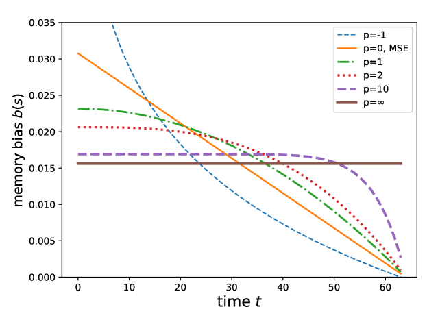
Figure 1: Normalized memory bias for different $p$

It can be seen that as $p$ goes to $\infty$, the memory bias flattened. In the limiting case, it’s the unbiased last-term-only loss. Therefore, by properly tuning the parameter $p$ we can keep reduce the memory bias in the error.

Remark 3.6.

Since the gradient of network is usually evaluated by $\frac{\partial Error}{\partial w}\approx\frac{\partial Error}{\partial\rho}\frac{\partial\rho}{\partial w}$. It can be seen the bias in the error function will be inherited by the gradient. Properly tuning the temporally weighted error can also relax the vanishing gradient issue.

4 Numerical results

In this section, we use synthetic case (linear functional with polynomial decaying memory), copying problem [16], and text summarization problem [27] to justify the main results in the previous section. Notice that the numerical examples all focus on learning of long-term memory.

4.1 Synthetic case

We approximate the linear functional $\{H_{t}(x):t\in[0,T]\}$ with linear RNN and tanh RNN.

$$H_{t}(x):=\int_{0}^{t}\rho_{t-s}x_{s}ds,\quad t\in[0,T].$$ (19)

The memory function $\rho$ of the target functional is defined as $\rho(t)=\frac{1}{t^{2}}$, a decay function that exhibits a more gradual rate of decrease relative to the conventionally observed exponential decay in Recurrent Neural Networks.

Although the main theory is only established for linear RNN, it can be seen the result holds for general tanh RNN.

The memory errors shown in Table 1 and Table 2 are the mean absolute error in the memory function of linear functional:

$$\textrm{Memory difference}:=\int_{0}^{T}|\rho_{s}-\hat{\rho}_{s}|dx_{s}.$$ (20)

We show that as the power $p$ increased, after same number of epochs, the mean absolute memory error is smaller for larger $p$.

Table 1: The memory difference is monotonic in the weight function polynomial power $p$ for different hidden dimensions (linear RNN)

	$p=-1$	$p=0$	$p=1$	$p=2$	$p=\infty$
hidden dimension 4	0.167	0.136	0.120	0.111	0.085
hidden dimension 16	0.184	0.162	0.148	0.142	0.129
hidden dimension 64	0.169	0.103	0.084	0.074	0.054

Table 2: The memory difference is monotonic in the weight function polynomial power $p$ for different hidden dimensions (tanh RNN)

	$p=-1$	$p=0$	$p=1$	$p=2$	$p=\infty$
hidden dimension 4	0.248	0.235	0.227	0.224	0.218
hidden dimension 16	0.322	0.314	0.307	0.304	0.299
hidden dimension 64	0.427	0.435	0.420	0.410	0.039

4.2 Copying problem

Apart from the synthetic linear functional task, we consider another task which is difficult for the long memory [16]. This task is trained with a different loss function cross entropy. To show the generality of the temporally rescale error in learning long-term memory, we take temporal convolutional network [13] and state space model [28, 23] as the models to learn the copying problem.

In Figure 2, we show that larger $p$ gives a better accuracy when the loss is at the same value. As we rescale the error temporally but do not scale up the loss value, this is a fair comparison. The monotonicity in power $p$ indicates that the time-weighted loss is a more consistent error than the temporally uniform-weighted cross entropy in terms of learning long-memory task.

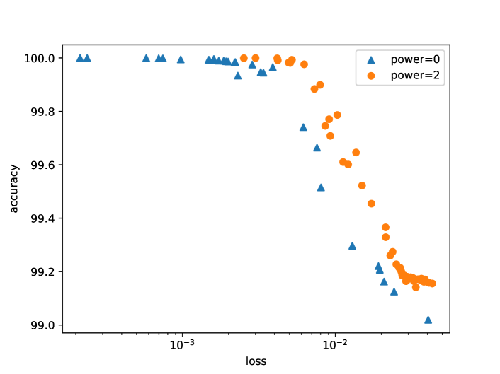
Figure 2: Copying Problem: Loss-Accuracy Graph for Temporal Convolutional Network. The graph indicates that with the same loss value, an increase in the power $p$ leads to higher accuracy. It should be highlighted that the two losses were trained with varying weights on cross-entropy, yet normalized to maintain a total weight of 1, ensuring a fair comparison.

In Figure 3, we show that with sufficient training, the accuracy of larger power $p$ can further increased. However, as shown in the power $p=10$ case, it should be notice that learning long-term memory is in general a more difficult task, therefore learning with a larger power $p$ can be relatively slower.

Figure 3: Copying problem, the validation accuracy for state space model (S4)

4.3 Text summarization

In this study, we bolstered the credibility of our methods by conducting additional validation using LCSTS [29]. LCSTS is an extensive compilation of Chinese text summarization datasets sourced from Sina Weibo, a prominent microblogging platform in China. Given the objective of generating summaries, our approach leverages long-term memory to proficiently capture and synthesize the complete content. For this purpose, we employed the T5-PEGASUS [30, 31] and CPT [32] models in our research. To demonstrate the effectiveness of our training, we evaluate the mean training rough-1 results after 10,000 training epochs, as shown in Table  3.

Table 3: The mean training rough-1 result on LCSTS after 10,000 training epochs. The rough-1 accuracy is monotonic in the weighted power $p$ for different models.

	$p=0$	$p=1$	$p=2$	$p=10$
T5-PEGASUS	0.4286	0.4342	0.4413	0.5212
CPT	0.4535	0.5656	0.5688	0.7354

4.4 Sensitivity of $p$

A natural question after the various numerical applications above is the sensitivity of the parameter $p$. Based on the main results in Section 3, the best parameter $p$ for linear functional among temporally positive-weighted error is the $\infty$. However, as we increase $p$ in the above copying problem, it can be seen the optimization is getting increasingly difficult.

In Figure 4 and Figure 5, we demonstrate with the linear functional task that the 1-step and 16-step results for loss decrease and gradient norm at the initialization. It shows that starting with a smaller $p$ usually improves the optimization. But to improve the learning of long-term memory, a large power $p$ is still required to reduce the memory bias.

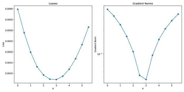
Figure 4: Sensitivity of parameter $p$ in the 1-step setting

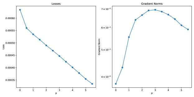
Figure 5: Sensitivity of parameter $p$ in the 16-step setting

5 Related work

Learning long-term memory in sequence modelling is crucial, as reflected in the emergence of long short-term memory (LSTM) model [9]. Initially proposed as a means to boost the ability of Recurrent Neural Networks (RNNs) to learn over extended periods, LSTM uses the gating mechanism to improve the long-term memory learning [33]. Similar approaches have been adopted in gated recurrent unit (GRU) [6]. The enhancement of the RNN’s and LSTM’s memory capabilities has been approached from a statistical perspective [34], leading to the proposal of setting the weight temporal decay at a polynomial rate. This polynomial decay corresponds to the memory function with polynomial decay in Equation 6. The LSTMp, as proposed by Chien et al. [35], introduces polynomial decay to the gate with the intention of improving long-term memory.

To better learn the long-term memory, it is necessary to have suitable memory metric. For linear functional [11], the memory function is characterized by the convolution kernel induced by the Riesz representation. For general nonlinear sequence to sequence relationship, there is no such representation. To gauge the effectiveness of differnt attempts to learn long memory, several benchmark tasks have been devised. A model’s long-term memory ability, for instance, can be measured using a copying problem, a task specifically designed for this purpose [16]. In the realm of language modelling, the LAMBADA dataset serves as a valuable tool for assessment [4]. A model’s performance on LAMBADA often serves as an indicator of its capability to capture information from extensive and diverse contexts. Further, memory capacity is introduced as another crucial metric for evaluating sequence modelling [36].

From the time series perspective, statistical literature proposes the use of relative error such as mean absolute percentage error (MAPE), mean absolute scaled error (MASE) [37].

$$\textrm{MASE}=\frac{1}{H}\sum_{i=1}^{H}\frac{|y_{T+i}-\hat{y}_{T+i}|}{\frac{1}{T+H-m}\sum_{j=m+1}^{T+H}|y_{j}-y_{j-m}|}.$$ (21)

However, MAPE mainly takes the scaling of the sequence into consideration. As changing the input output scale does not change the memory function scale or decay rate, the error from absolute error into relative error only removes the impact of sequence scale issue, which does not affect the definition of memory function or memory bias as they do not determine on the scale.

6 Limitation

Although the proper temporal rescaling can improve the performance of learning long memory, this method requires the output to be sequential. Our method is currently limited to temporally positive-weighted error. The borader weight family such as nonlinear combination of relative error might further aid the learning of long-term memory.

7 Conclusion

In this paper, we study the bias of mean absolute/squared error towards short-term memory. We evaluate the memory bias based on the generalized memory function, which is a natural extension of the linear functional’s representation. Moreover, it is shown that such a memory bias exist across all temporally positive-weighted errors. The bias problem can be relaxed by choosing a suitable weight. The bias-variance trade-off is discussed when the output sequence is susceptible to noise. Numerical experiments from synthetic dataset (linear functional) are conducted to validate the results. In particular, we show the discovery is not limited to synthetic case and recurrent neural networks. General sequence modelling such as copying problem and language modelling learned by other network structures can also benefit from the application of proper temporally positive-weighted error.

Appendix A Linear functional and corresponding theoretical results

In this section, we give the definitions of several properties for linear functional.

Definitions for linear functional

1. (Linearity) $H_{t}$ is linear if for any $c_{1},c_{2}\in\mathbb{R}$ and $\mathbf{x},\mathbf{x}^{\prime}\in\mathcal{X}$, $H_{t}(c_{1}\mathbf{x}+c_{2}\mathbf{x}^{\prime})=c_{1}H_{t}(\mathbf{x})+c_{2}H_{t}(\mathbf{x}^{\prime})$.

2. (Continuous) $H_{t}$ is continuous if for any $\mathbf{x},^{\prime}\mathbf{x}\in\mathcal{X}$, $\lim_{{\mathbf{x}^{\prime}\to\mathbf{x}}}|H_{t}(\mathbf{x}^{\prime})-H_{t}(\mathbf{x})|=0$.

3. (Time-homogeneous) $\mathbf{H}=\{H_{t}:t\in\mathbb{R}\}$ is time-homogeneous if the input-output relationship interchanges with time shift: let $[S_{\tau}(\mathbf{x})]_{t}=x_{t-\tau}$ be a shift operator, then $\mathbf{H}(S_{\tau}\mathbf{x})=S_{\tau}\mathbf{H}(\mathbf{x})$.

4. (Causal) $H_{t}$ is causal if it does not depend on future values of the input. That is, if $\mathbf{x},\mathbf{x}^{\prime}$ satisfy $x_{t}=x_{t}^{\prime}$ for any $t\leq T$, then $H_{t}(\mathbf{x})=H_{t}(\mathbf{x}^{\prime})$ for any $t\leq T$.

5. (Regualrity) $H_{t}$ is regular if for any sequence $\{\mathbf{x}^{(k)}:k\in\mathbb{N}\}$ such that $x^{(k)}_{s}\to 0$ for almost every $s\in\mathbb{R}$, then $\lim_{k\to\infty}H_{t}(\mathbf{x}^{(k)})=0.$

The linearity is a strong assumption as most of the general sequence to sequence relationship is nonlinear. The continuity, time-homogeneous and regularity are general properties that nice predictable sequence with temporal structures should have.

Riesz representation theorem

Theorem A.1 (Riesz-Markov-Kakutani representation theorem).

Assume $H:\mathcal{X}\mapsto\mathbb{R}$ is a linear and continuous functional. Then there exists a unique, vector-valued, regular, countably additive signed measure $\mu$ on $\mathbb{R}$ such that

$$H(\mathbf{x})=\int_{\mathbb{R}}x_{s}^{\top}d\mu(s)=\sum_{i=1}^{d}\int_{\mathbb{R}}x_{s,i}d\mu_{i}(s).$$ (22)

In addition, we have $\|H\|:=\sup_{\|\mathbf{x}\|_{\mathcal{X}}\leq 1}|H(\mathbf{x})|=\|\mu\|_{1}(\mathbb{R}):=\sum_{i}|\mu_{i}|(\mathbb{R}).$

Appendix B Proof for Theorem 3.3

Consider the following weighted squared error

$$\textrm{Error}^{\textrm{TPE}}=\int_{0}^{T}w(t)|y_{t}-\hat{y}_{t}|dt.$$ (23)

It can be seen that

$$\mathcal{E}^{\textrm{TPE}} =\mathbb{E}_{\mathbf{x}}\textrm{Error}^{\textrm{TPE}}=\mathbb{E}_{\mathbf{x}}\int_{0}^{T}w(t)\left|\int_{0}^{t}(\rho_{t-s}-\hat{\rho}_{t-s})x_{s}ds\right|dt$$ (24)

$$=c_{0}\int_{0}^{T}w(t)\left(\int_{0}^{t}\left|\rho_{t-s}-\hat{\rho}_{t-s}\right|ds\right)dt$$ (25)

$$=c_{0}\int_{0}^{T}w(t)\left(\int_{0}^{t}\left|\rho_{s}-\hat{\rho}_{s}\right|ds\right)dt$$ (26)

$$=c_{0}\int_{0}^{T}\int_{0}^{t}w(t)\left|\rho_{s}-\hat{\rho}_{s}\right|dsdt$$ (27)

$$=c_{0}\int_{0}^{T}\int_{s}^{T}w(t)\left|\rho_{s}-\hat{\rho}_{s}\right|dtds$$ (28)

$$=c_{0}\int_{0}^{T}\left(\int_{s}^{T}w(t)dt\right)\left|\rho_{s}-\hat{\rho}_{s}\right|ds$$ (29)

Appendix C Additional numerical result

In addition to the temporal convolution network and state-space model (SSM), we also compare the performance of time-weighted error on attention-based transformer (see Figure 6). Moreover, it can be seen the gradient norm for time-weighted error with $p=2$ is larger and it relatively robust against the typical vanishing gradient issue.

Figure 6: Copying problem, the validation accuracy for attention-based transformer

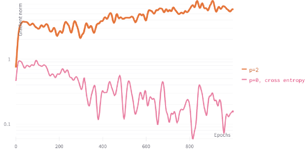
Figure 7: Copying problem, the gradient norm for attention-based transformer

Appendix D Numerical experiment details

In this section, the setups for different numerical experiments are included.

D.1 Synthetic linear functional

We use linear and tanh RNNs to learn linear functionals with polynomial decaying memory. The memory function of linear functional is $\displaystyle\rho(t)=\frac{1}{t^{1.1}}$. Sequence length is 64. Time discretization is $\Delta t=0.1$. Train batch size and test batch size are 512 and 2048. Optimizer is Adam with learning rate 0.001. The training dataset is manually constructed with size 131072 while the test dataset is of size 32768.

D.2 Copying problem

The copying problem is conducted based on temporal convolution network as well as state-space models. The temporally uniform-weighted version ($w(t)\equiv 1$) is implemented based on the model provided in both repo. The data generation and model construction is generally the same as the example presented in the repo.

D.3 Text summarization

The text summarization process relies on the utilization of an open-source repository named "t5-pegasus-pytorch". We make use of the model available in this repository and implement a different optimizer, as described in Section 2. By leveraging the existing model and incorporating our own optimizer, we aim to enhance the performance of the text summarization process.

D.4 Bias-variance tradeoff

The bias-variance tradeoff is discussed based on the experiments for synthetic linear functional. The power $p$ is tested over $[0,\frac{1}{2},1,\dots,\frac{11}{2}]$. The optimizer for 1-step and 16-step training is SGD with learning rate 0.1. Most of the training set is the same as synthetic linear functional.

Appendix E Discussion on the difficulty of training when $p$ is large

As is shown in Figure 3, we observe that the accuracy of larger $p$ is increasing much slower than smaller $p$. We emphaisze that this result does not contradict the general rule that larger $p$ shall give less memory bias on the short term memory. This result is verified as we prolong the training from 1500 epochs to 6000 epochs, the accuracy raises to 0.4512 which is larger than the smaller $p$. The higher accuracy at later stage validates the hypothesis presented in Figure 4 and Figure 5.

Appendix F Computing resources

The experiments are conducted on a 20.04 Ubuntu server with 4 RTX 3090 GPUs.

References

- Connor et al. [1994] Jerome T. Connor, R. Douglas Martin, and Les E. Atlas. Recurrent neural networks and robust time series prediction. IEEE transactions on neural networks, 5(2):240–254, 1994.
- Wu et al. [2016] Yonghui Wu, Mike Schuster, Zhifeng Chen, Quoc V. Le, Mohammad Norouzi, Wolfgang Macherey, Maxim Krikun, Yuan Cao, Qin Gao, Klaus Macherey, Jeff Klingner, Apurva Shah, Melvin Johnson, Xiaobing Liu, Łukasz Kaiser, Stephan Gouws, Yoshikiyo Kato, Taku Kudo, Hideto Kazawa, Keith Stevens, George Kurian, Nishant Patil, Wei Wang, Cliff Young, Jason Smith, Jason Riesa, Alex Rudnick, Oriol Vinyals, Greg Corrado, Macduff Hughes, and Jeffrey Dean. Google’s Neural Machine Translation System: Bridging the Gap between Human and Machine Translation, October 2016.
- Graves et al. [2013] Alex Graves, Abdel-rahman Mohamed, and Geoffrey Hinton. Speech Recognition with Deep Recurrent Neural Networks, March 2013.
- Paperno et al. [2016] Denis Paperno, Germán Kruszewski, Angeliki Lazaridou, Ngoc Quan Pham, Raffaella Bernardi, Sandro Pezzelle, Marco Baroni, Gemma Boleda, and Raquel Fernández. The LAMBADA dataset: Word prediction requiring a broad discourse context. In Proceedings of the 54th Annual Meeting of the Association for Computational Linguistics (Volume 1: Long Papers), pages 1525–1534, Berlin, Germany, August 2016. Association for Computational Linguistics. doi: 10.18653/v1/P16-1144.
- Kirkpatrick et al. [2017] James Kirkpatrick, Razvan Pascanu, Neil Rabinowitz, Joel Veness, Guillaume Desjardins, Andrei A. Rusu, Kieran Milan, John Quan, Tiago Ramalho, Agnieszka Grabska-Barwinska, Demis Hassabis, Claudia Clopath, Dharshan Kumaran, and Raia Hadsell. Overcoming catastrophic forgetting in neural networks. Proceedings of the National Academy of Sciences, 114(13):3521–3526, March 2017. ISSN 0027-8424, 1091-6490. doi: 10.1073/pnas.1611835114.
- Cho et al. [2014] Kyunghyun Cho, Bart van Merrienboer, Caglar Gulcehre, Dzmitry Bahdanau, Fethi Bougares, Holger Schwenk, and Yoshua Bengio. Learning Phrase Representations using RNN Encoder-Decoder for Statistical Machine Translation. Proceedings of the 2014 Conference on Empirical Methods in Natural Language Processing, pages 1724–1734, September 2014.
- Informatik et al. [2003] Fakultit Informatik, Y. Bengio, Paolo Frasconi, and Jfirgen Schmidhuber. Gradient Flow in Recurrent Nets: The Difficulty of Learning Long-Term Dependencies. A Field Guide to Dynamical Recurrent Neural Networks, March 2003.
- Rumelhart et al. [1986] David E. Rumelhart, Geoffrey E. Hinton, and Ronald J. Williams. Learning representations by back-propagating errors. Nature, 323(6088):533–536, October 1986. ISSN 1476-4687. doi: 10.1038/323533a0.
- Hochreiter and Schmidhuber [1997] Sepp Hochreiter and Jürgen Schmidhuber. Long Short-term Memory. Neural computation, 9:1735–80, December 1997. doi: 10.1162/neco.1997.9.8.1735.
- Pascanu et al. [2013] Razvan Pascanu, Tomas Mikolov, and Yoshua Bengio. On the difficulty of training recurrent neural networks. In Proceedings of the 30th International Conference on Machine Learning, pages 1310–1318. PMLR, May 2013.
- Li et al. [2022] Zhong Li, Jiequn Han, Weinan E, and Qianxiao Li. Approximation and Optimization Theory for Linear Continuous-Time Recurrent Neural Networks. Journal of Machine Learning Research, 23(42):1–85, 2022. ISSN 1533-7928.
- Wang et al. [2023] Shida Wang, Zhong Li, and Qianxiao Li. Inverse Approximation Theory for Nonlinear Recurrent Neural Networks, May 2023.
- Bai et al. [2018] Shaojie Bai, J. Zico Kolter, and Vladlen Koltun. An Empirical Evaluation of Generic Convolutional and Recurrent Networks for Sequence Modeling. https://arxiv.org/abs/1803.01271v2, March 2018.
- Vaswani et al. [2017] Ashish Vaswani, Noam Shazeer, Niki Parmar, Jakob Uszkoreit, Llion Jones, Aidan N Gomez, Łukasz Kaiser, and Illia Polosukhin. Attention is All you Need. In Advances in Neural Information Processing Systems, volume 30. Curran Associates, Inc., 2017.
- Chang et al. [2018] Bo Chang, Minmin Chen, Eldad Haber, and Ed H. Chi. AntisymmetricRNN: A Dynamical System View on Recurrent Neural Networks. In International Conference on Learning Representations, December 2018.
- Arjovsky et al. [2016] Martin Arjovsky, Amar Shah, and Yoshua Bengio. Unitary Evolution Recurrent Neural Networks. In Proceedings of The 33rd International Conference on Machine Learning, pages 1120–1128. PMLR, June 2016.
- Li et al. [2018] Shuai Li, Wanqing Li, Chris Cook, Ce Zhu, and Yanbo Gao. Independently Recurrent Neural Network (IndRNN): Building A Longer and Deeper RNN. In 2018 IEEE/CVF Conference on Computer Vision and Pattern Recognition, pages 5457–5466, June 2018. doi: 10.1109/CVPR.2018.00572.
- Jose et al. [2018] Cijo Jose, Moustapha Cisse, and Francois Fleuret. Kronecker Recurrent Units. In Proceedings of the 35th International Conference on Machine Learning, pages 2380–2389. PMLR, July 2018.
- Lezcano-Casado and Martínez-Rubio [2019] Mario Lezcano-Casado and David Martínez-Rubio. Cheap Orthogonal Constraints in Neural Networks: A Simple Parametrization of the Orthogonal and Unitary Group. In Proceedings of the 36th International Conference on Machine Learning, pages 3794–3803. PMLR, May 2019.
- Rusch et al. [2022] T. Konstantin Rusch, Siddhartha Mishra, N. Benjamin Erichson, and Michael W. Mahoney. Long Expressive Memory for Sequence Modeling. In International Conference on Learning Representations, January 2022.
- Rusch and Mishra [2022] T. Konstantin Rusch and Siddhartha Mishra. Coupled Oscillatory Recurrent Neural Network (coRNN): An accurate and (gradient) stable architecture for learning long time dependencies. In International Conference on Learning Representations, February 2022.
- Gu et al. [2020] Albert Gu, Tri Dao, Stefano Ermon, Atri Rudra, and Christopher Ré. HiPPO: Recurrent Memory with Optimal Polynomial Projections. In Advances in Neural Information Processing Systems, volume 33, pages 1474–1487. Curran Associates, Inc., 2020.
- Smith et al. [2023] Jimmy T. H. Smith, Andrew Warrington, and Scott Linderman. Simplified State Space Layers for Sequence Modeling. In International Conference on Learning Representations, February 2023.
- Romero et al. [2022] David W. Romero, Anna Kuzina, Erik J. Bekkers, Jakub Mikolaj Tomczak, and Mark Hoogendoorn. CKConv: Continuous Kernel Convolution For Sequential Data. In International Conference on Learning Representations, January 2022.
- Li et al. [2021] Zhong Li, Jiequn Han, Weinan E, and Qianxiao Li. On the Curse of Memory in Recurrent Neural Networks: Approximation and Optimization Analysis. In International Conference on Learning Representations, March 2021.
- Jiang et al. [2023] Haotian Jiang, Qianxiao Li, Zhong Li Null, and Shida Wang. A Brief Survey on the Approximation Theory for Sequence Modelling. Journal of Machine Learning, 2(1):1–30, June 2023. ISSN 2790-203X, 2790-2048. doi: 10.4208/jml.221221.
- Liu and Lapata [2019] Yang Liu and Mirella Lapata. Text Summarization with Pretrained Encoders. In Proceedings of the 2019 Conference on Empirical Methods in Natural Language Processing and the 9th International Joint Conference on Natural Language Processing (EMNLP-IJCNLP), pages 3730–3740, Hong Kong, China, November 2019. Association for Computational Linguistics. doi: 10.18653/v1/D19-1387.
- Gu et al. [2021] Albert Gu, Isys Johnson, Karan Goel, Khaled Saab, Tri Dao, Atri Rudra, and Christopher Ré. Combining Recurrent, Convolutional, and Continuous-time Models with Linear State Space Layers. In Advances in Neural Information Processing Systems, volume 34, pages 572–585. Curran Associates, Inc., 2021.
- Hu et al. [2015] Baotian Hu, Qingcai Chen, and Fangze Zhu. LCSTS: A Large Scale Chinese Short Text Summarization Dataset. In Proceedings of the 2015 Conference on Empirical Methods in Natural Language Processing, pages 1967–1972, Lisbon, Portugal, September 2015. Association for Computational Linguistics. doi: 10.18653/v1/D15-1229.
- Xue et al. [2021] Linting Xue, Noah Constant, Adam Roberts, Mihir Kale, Rami Al-Rfou, Aditya Siddhant, Aditya Barua, and Colin Raffel. mT5: A Massively Multilingual Pre-trained Text-to-Text Transformer. In Proceedings of the 2021 Conference of the North American Chapter of the Association for Computational Linguistics: Human Language Technologies, pages 483–498, Online, June 2021. Association for Computational Linguistics. doi: 10.18653/v1/2021.naacl-main.41.
- Zhang et al. [2020] Jingqing Zhang, Yao Zhao, Mohammad Saleh, and Peter Liu. PEGASUS: Pre-training with Extracted Gap-sentences for Abstractive Summarization. In Proceedings of the 37th International Conference on Machine Learning, pages 11328–11339. PMLR, November 2020.
- Shao et al. [2022] Yunfan Shao, Zhichao Geng, Yitao Liu, Junqi Dai, Hang Yan, Fei Yang, Li Zhe, Hujun Bao, and Xipeng Qiu. CPT: A Pre-Trained Unbalanced Transformer for Both Chinese Language Understanding and Generation. Arxiv: 2109.05729, July 2022. doi: 10.1007/s11432-021-3536-5.
- Chen et al. [2018] Minmin Chen, Jeffrey Pennington, and Samuel Schoenholz. Dynamical Isometry and a Mean Field Theory of RNNs: Gating Enables Signal Propagation in Recurrent Neural Networks. In Proceedings of the 35th International Conference on Machine Learning, pages 873–882. PMLR, July 2018.
- Zhao et al. [2020] Jingyu Zhao, Feiqing Huang, Jia Lv, Yanjie Duan, Zhen Qin, Guodong Li, and Guangjian Tian. Do RNN and LSTM have Long Memory? In Proceedings of the 37th International Conference on Machine Learning, pages 11365–11375. PMLR, November 2020.
- Chien et al. [2021] Hsiang-Yun Sherry Chien, Javier S. Turek, Nicole Beckage, Vy A. Vo, Christopher J. Honey, and Ted L. Willke. Slower is Better: Revisiting the Forgetting Mechanism in LSTM for Slower Information Decay. Arxiv: 2105.05944, May 2021. doi: 10.48550/arXiv.2105.05944.
- Gallicchio [2018] Claudio Gallicchio. Short-term Memory of Deep RNN. Arxiv:1802.00748, February 2018. doi: 10.48550/arXiv.1802.00748.
- Hyndman [2006] Rob Hyndman. Another Look at Forecast Accuracy Metrics for Intermittent Demand. Foresight: The International Journal of Applied Forecasting, 4:43–46, January 2006.