Bifurcation domains from any high eigenvalue for an overdetermined elliptic problem

Abstract

In this paper, we consider the following overdetermined eigenvalue problem on an unbounded domain $\Omega\subset\mathbb{R}^{N+1}$ with $N\geq 1$

$$\left\{\begin{array}[]{ll}-\Delta u=\lambda u&\text{in}\,\,\Omega,\\ u=0&\text{on}\,\,\partial\Omega,\\ \partial_{\nu}u=\text{const}&\text{on}\,\,\partial\Omega.\end{array}\right.$$

Let $\lambda_{k}$ be the $k$-th eigenvalue of the zero-Dirichlet Laplacian on the unit ball for any $k\in\mathbb{N^{+}}$ with $k\geq 3$. We can construct $k$ smooth families of nontrivial unbounded domains $\Omega$, bifurcating from the straight cylinder, which admit a nonsymmetric solution with changing the sign by $k-1$ times to the overdetermined problem. While the existence of such domains for $k=1,2$ has been well-known, to the best of our knowledge this is the first construction for any positive integer $k\geq 3$. Due to the complexity of studying high eigenvalue problem, our proof involves some novel analytic ingredients. These results can be regarded as counterexamples to the Berenstein conjecture on unbounded domain.

Keywords: Berenstein conjecture; Overdetermined problem; Bifurcation; Eigenvalue; Unbounded domain

AMS Subjection Classification(2020): 35B05; 35B32; 35N05

1 Introduction

Overdetermined elliptic problem has important application background in plasma physics [27], nuclear reactors [3] and tomography [26]. A celebrated theorem of Serrin [24] asserts that one overdetermined condition on the boundary is enough to obtain the radial symmetry solution of the following overdetermined torsion problem

$$\left\{\begin{array}[]{ll}\Delta u+1=0&\text{in}\,\,\Omega,\\ u>0&\text{in}\,\,\Omega,\\ u=0&\text{on}\,\,\partial\Omega,\\ \partial_{\nu}u=\text{const}&\text{on}\,\,\partial\Omega\end{array}\right.$$ (1.1)

with $\Omega$ being a bounded domain of class $C^{2}$ and $\nu$ being the unit outward normal vector about $\partial\Omega$. That is to say, if there is a solution to problem (1.1) on bounded domain, then $\Omega$ must be a ball. Subsequently, for the more general overdetermined elliptic problem

$$\left\{\begin{array}[]{ll}\Delta u+f(u)=0&\text{in}\,\,\Omega,\\ u>0&\text{in}\,\,\Omega,\\ u=0&\text{on}\,\,\partial\Omega,\\ \partial_{\nu}u=\text{const}&\text{on}\,\,\partial\Omega,\end{array}\right.$$ (1.2)

where $\Omega\subset\mathbb{R}^{N}$ is a given regular domain and $f$ is a Lipschitz function, Berestycki, Caffarelli and Nirenberg [6] proposed the following conjecture.

BCN Conjecture. If $\Omega$ is a smooth domain and $\mathbb{R}^{N}\setminus\overline{\Omega}$ is connected such that there exists a bounded solution to problem (1.2), then $\Omega$ is either a ball, a half-space, a generalized cylinder $B^{k}\times\mathbb{R}^{N-k}$ where $B^{k}$ is a ball in $\mathbb{R}^{k}$, or the complement of one of them.

It is well known that many positive answers to the BCN conjecture have been given in bounded domain by using the so-called moving plane method. If $f$ is a Lipschitz function and $\Omega$ is bounded, Pucci and Serrin [18] proved that BCN Conjecture is holding. Under some suitable assumptions, Berestycki, Caffarelli and Nirenberg [6] proved that if problem (1.2) admits a smooth bounded solution, then $\Omega$ is a half-space. If $\Omega$ is a globally Lipschitz smooth epigraph of $\mathbb{R}^{N}$ with $N=2$, $3$, Farina and Valdinoci [11] proved that $\Omega$ admits a positive solution $u$ to problem (1.2) with $C^{1}$ bistable nonlinearity must be a half-space and $u$ must be a function of only one variable, which can be seen as a confirm answer to BCN or Berenstein conjecture on unbounded domain. When $N=2$, with some more weaker conditions on $f$ and $u$, Ros, Ruiz and Sicbaldi [20] proved that the BCN Conjecture is valid on $C^{1,\alpha}$ domain whose boundary is unbounded and connected. With some suitable conditions, Serrin’s result is also valid on some exterior domains [1, 19].

In two surprising papers however, Sicbaldi [25] constructed a counter-example to BCN Conjecture and proved that the cylinder $B_{1}^{N}\times\mathbb{R}$ with $N\geq 2$ can be perturbed to an unbounded domain whose boundary is a periodic hypersurface of revolution with respect to the $\mathbb{R}$-axis, such that the problem

$$\left\{\begin{array}[]{ll}\Delta u+\lambda u=0&\text{in}\,\,\Omega,\\ u=0&\text{on}\,\,\partial\Omega,\\ \partial_{\nu}u=\text{const}&\text{on}\,\,\partial\Omega\end{array}\right.$$

has a bounded positive solution, where $B_{1}^{N}$ is the unit ball in $\mathbb{R}^{N}$ centered at the origin. Subsequently, Schlenk and Sicbaldi [23] further proved that the above conclusion is valid for $N=1$ and these new extremal domains belong to a smooth bifurcation family of domains. It is worth noting that these nontrivial solutions constructed in [25] can be regarded as the perturbation of the eigenfunction $\phi_{1}$ corresponding to the first eigenvalue $\lambda_{1}$ of the Laplacian on the unit ball, which are positive. Recently, we [9] prove the existence of two smooth families of unbounded domains in $\mathbb{R}^{N+1}$ such that the above overdetermined eigenvalue problem has a sign-changing solution, which can be seen the perturbation of the eigenfunction corresponding to $\lambda_{2}$.

The natural question is whether can we obtain sign-changing solutions by perturbing eigenfunction function corresponding to any high eigenvalue $\lambda_{k}$? In this paper, we managed to show the existence of nontrivial sign-changing solutions bifurcating from the eigenfunction $\phi_{k}$ corresponding to any high eigenvalue $\lambda_{k}$ of the Laplacian on the unit ball for $k\geq 3$. In fact, these results also can be seen as counter-examples to the following Conjecture on unbounded domains due to Berenstein [3, 4, 5].

Berenstein conjecture. Let $\Omega$ be a bounded $C^{2,\alpha}$ domain in $\mathbb{R}^{N+1}$ with $\alpha\in(0,1)$. If there exists a nontrivial solution $u$ of the overdetermined eigenvalue problem

$$\left\{\begin{array}[]{ll}\Delta u+\lambda u=0&\text{in}\,\,\Omega,\\ u=0&\text{on}\,\,\partial\Omega,\\ \partial_{\nu}u=\text{const}&\text{on}\,\,\partial\Omega,\end{array}\right.$$ (1.3)

then $\Omega$ is a ball, where $\nu$ is the unit outer normal on $\partial\Omega$.

Our main results are stated as follows.

Theorem 1.1. Let $k\in\mathbb{N^{+}}$ with $k\geq 3$ and assume that $\mathcal{C}^{2,\alpha}_{\text{even},0}\left(\mathbb{R}/2\pi\mathbb{Z}\right)$ is the space of even $2\pi$-periodic $\mathcal{C}^{2,\alpha}$ functions of mean zero. There exist a positive number $T_{1,*}$ with

$$T_{1,*}\in\left(\frac{2\pi}{\sqrt{\lambda_{k}}},\frac{2\pi}{\sqrt{\lambda_{k}-\lambda_{1}}}\right)$$

and a smooth map

$$(-\varepsilon,\varepsilon)\rightarrow\mathcal{C}^{2,\alpha}_{\text{even},0}\left(\mathbb{R}/2\pi\mathbb{Z}\right)\times\mathbb{R}:s\mapsto\left(w_{s},T_{s}\right)$$

with $w_{0}=0$, $T_{0}=T_{1,*}$ such that for each $s\in(-\varepsilon,\varepsilon)$, the problem (1.3) has a sign-changing $T_{s}$-periodic solution $u_{s}\in\mathcal{C}^{2,\alpha}\left(\Omega_{s}\right)$ on the modified cylinder

$$\Omega_{s}=\left\{(x,t)\in\mathbb{R}^{N}\times\mathbb{R}:|x|<1+s\cos\left(\frac{2\pi}{T_{s}}t\right)+sw_{s}\left(\frac{2\pi}{T_{s}}t\right)\right\}$$

for $N\geq 2$. Moreover, there exist $k-1$ $T_{s}$-periodic functions $r_{j}\in\mathcal{C}^{2,\alpha}\left(\mathbb{R}\right)$ with

$$r_{j}(t):\mathbb{R}\longrightarrow\left(0,1+s\cos\left(\frac{2\pi}{T_{s}}t\right)+sw_{s}\left(\frac{2\pi}{T_{s}}t\right)\right),$$

where $j\in\{1,\ldots,k-1\}$ and $r_{1}(t)<\cdots<r_{k-1}(t)$, such that $u_{s}\left(r_{j}(t),t\right)=0$.

Different from $T_{1,*}$, we further obtain the other $k-1$ bifurcation points which may be corresponding to high-dimensional kernel space.

Theorem 1.2. Under the assumptions of Theorem 1.1, there exist $k-1$ positive numbers $T_{2,*}$, $\ldots$, $T_{k,*}$ with

$$\,\,T_{i,*}\in\left(\frac{2\pi}{\sqrt{\lambda_{k}-\lambda_{i-1}}},\frac{2\pi}{\sqrt{\lambda_{k}-\lambda_{i}}}\right)$$

for each $i\in\{2,\ldots,k\}$ and $k-1$ smooth maps

$$(-\varepsilon,\varepsilon)\rightarrow\mathcal{C}^{2,\alpha}_{\text{even},0}\left(\mathbb{R}/2\pi\mathbb{Z}\right)\times\mathbb{R}:s\mapsto\left(w_{s},T_{s}\right)$$

with $w_{0}=0$, $T_{i,0}=T_{i,*}$ such that for each $s\in(-\varepsilon,\varepsilon)$, the problem (1.3) has a sign-changing $T_{s}$-periodic solution $u_{s}\in\mathcal{C}^{2,\alpha}\left(\Omega_{s}\right)$ on the modified cylinder

$$\Omega_{s}=\left\{(x,t)\in\mathbb{R}^{N}\times\mathbb{R}:|x|<1+s\left(\beta\cos\left(\frac{2\pi}{T_{s}}t\right)+\sum_{n=1}^{m}\gamma_{n}\cos\left(\frac{2l_{j_{n}}\pi}{T_{s}}t\right)\right)+sw_{s}\left(\frac{2\pi}{T_{s}}t\right)\right\},$$

for $N\geq 2$, where either $\beta$, $\gamma_{n}$ are nonzero constants with $\beta^{2}+\sum_{n=1}^{m}\gamma_{n}^{2}=1$ if there exist $m$ elements of $\{1,\ldots,i-1\}$ with $m\leq i-1$, which are denoted by $j_{n}$ with $n\in\{1,\ldots,m\}$, such that $T_{i,*}=l_{j_{n}}T_{j_{n},*}$ for some $l_{j_{n}}\in\mathbb{N}$ with $l_{j_{n}}\geq 2$, or $\beta=1$ and $\gamma_{n}=0$ if $T_{i,*}\neq lT_{j,*}$ for every $j\in\{1,\ldots,i-1\}$ and any $l\in\mathbb{N}$ with $l\geq 2$. Moreover, there exist $k-1$ $T_{s}$-periodic functions $r_{j}\in\mathcal{C}^{2,\alpha}\left(\mathbb{R}\right)$ for $j\in\{1,\ldots,k-1\}$ with

$$r_{j}(t):\mathbb{R}\longrightarrow\left(0,1+s\left(\beta\cos\left(\frac{2\pi}{T_{s}}t\right)+\sum_{n=1}^{m}\gamma_{n}\cos\left(\frac{2l_{j_{n}}\pi}{T_{s}}t\right)\right)+sw_{s}\left(\frac{2\pi}{T_{s}}t\right)\right)$$

and

$$r_{1}(t)<\cdots<r_{k-1}(t),$$

such that $u_{s}\left(r_{j}(t),t\right)=0$.

Indeed, these results also can be taken regard as a generalization of [9, Theorems 1.1–1.2], however some essential difficulties brought by high eigenvalue are intractable. For one-dimensional kernel space case, we mainly use the classical Crandall-Rabinowitz bifurcation theorem. However, if there holds that $T_{i,*}=l_{j_{n}}T_{j_{n},*}$ for some $l_{j_{n}}\in\mathbb{N}$ with $l_{j_{n}}\geq 2$, then the kernel space corresponding to $T_{i,*}$ is high-dimensional, which leads to that the classical Crandall-Rabinowitz bifurcation theorem is not available. Fortunately, a new Crandall-Rabinowitz type local bifurcation theorem of high-dimensional kernels due to [9] seems an efficient tool at this time. From [9, Remark 1.3] we know that high-dimensional kernel bifurcation does not occur for $N=1$. While we will see that high-dimensional kernel bifurcation must occur for $N=1$ in this paper (see Remark 5.2). To the best of our knowledge, this is the first concrete example of bifurcation with high-dimensional kernel. Although the whole idea of proof is an extension of our method in [9], compared with the case of [9], the analysis of Bessel functions developed here is more delicate since there are more zero points. The spectral study is more complex in this case, and we achieve the existence of $k-1$ branches of bifurcation by implementing bifurcation techniques. Constructing the nontrivial sign-changing solution to some overdetermined problems has attracted a lot of attention among mathematicians recently (see [15, 21]), while it is worth noting that the method and problem developed here are different from those of [15, 21] as pointed in [9]. After the completion of the current paper, we learned of the paper [16] by Minlend, which establishes the existence of nontrivial unbounded domains such that the problem (1.3) admits sign-changing eigenfunctions by a different approach. However, the bifurcation domains found by Minlend are less than ours and the phenomenon of high-dimensional bifurcation kernel can’t occur in [16].

The rest of this paper is arranged as follows. In Section 2, we rephrase the problem by giving the definition of the Dirichlet-to-Neumann operator $F$ and its linearization $F_{v}(0,T)$. In addition, we also show some basic conclusions of Bessel functions that will be applied later. The properties of spectral $\sigma_{1}(T)$ for the linearized operator $F_{v}(0,T)$ are obtained in Section 3 and the proofs of Theorems 1.1–1.2 are given in Section 4 for $N\geq 2$. In Section 5, we show that the results of Theorems 1.1–1.2 are also valid for $N=1$ where the method used is different from the case of $N\geq 2$.

2 Preliminaries

2.1 The formulation of the bifurcation problem

Consider the following eigenvalue problem

$$\left\{\begin{array}[]{ll}\Delta u+\lambda u=0&\text{in}\,\,B_{1},\\ u=0&\text{on}\,\,\partial B_{1}.\end{array}\right.$$ (2.1)

It is well known (see [7, 13] or [28, p. 269]) that problem (2.1) has a sequence eigenvalues $0<\lambda_{1}<\lambda_{2}<\cdots<\lambda_{k}\nearrow+\infty$. Let $\overline{\phi}_{k}$ be the corresponding eigenfunction to $\lambda_{k}$ with $\int_{B_{1}}\overline{\phi}_{k}^{2}\,\text{d}x=1/\left(2\pi\right)$ and $\overline{\phi}_{k}(0)>0$. From now on, we use $C$ or $C_{k}$ to denote some positive constant whose exact value may change from line to line.

In particular, for $N=1$, we have that

$$\lambda_{k}=\frac{(2k-1)^{2}\pi^{2}}{4}\,\,\,\text{and}\,\,\,\overline{\phi}_{k}(r)=\frac{1}{\sqrt{2\pi}}\cos\left(\frac{(2k-1)\pi}{2}r\right).$$ (2.2)

For $N=3$, it follows from [9, Lemma 2.1] that

$$\lambda_{k}=k^{2}\pi^{2}\,\,\,\text{and}\,\,\,C_{k}\overline{\phi}_{k}(r)=\left\{\begin{array}[]{ll}\frac{\sin(k\pi r)}{r}&\text{if}\,\,r>0,\\ k\pi&\text{if}\,\,r=0,\end{array}\right.$$ (2.3)

where $C_{k}$ is chosen such that $\int_{B_{1}}\overline{\phi}_{k}^{2}\,\text{d}x=1/\left(2\pi\right)$. Clearly, we see that $\left(\lambda_{k},{\phi}_{k}(x,t)\right)$ with ${\phi}_{k}(x,t)=\overline{\phi}_{k}(x)$ is also a solution pair of

$$\left\{\begin{array}[]{ll}\Delta_{\mathring{g}}{\phi}+\lambda{\phi}=0&\text{in}\,\,C_{1}^{T},\\ {\phi}=0&\text{on}\,\,\partial C_{1}^{T},\end{array}\right.$$ (2.4)

where $\mathring{g}$ is the Euclidean metric and

$$C_{1}^{T}=\left\{(x,t)\in\mathbb{R}^{N}\times\mathbb{R}/T\mathbb{Z}:|x|<1\right\}.$$

It is obvious that

$$\int_{C_{1}^{2\pi}}{\phi}_{k}^{2}\,\text{d}\text{vol}_{\mathring{g}}=1.$$

As $\phi_{k}$ does not depend on $t$ and it is radial, we can denote $\phi_{k}(x,t)$ by $\phi_{k}(r)$ with $r=|x|$.

We now transform the aim problem (1.3) into an abstract operator equation. For any $v\in\mathcal{C}^{2,\alpha}_{\text{even},0}\left(\mathbb{R}/2\pi\mathbb{Z}\right)$ with $v>-1$, define

$$C_{1+v}^{T}=\left\{(x,t)\in\mathbb{R}^{N}\times\mathbb{R}/T\mathbb{Z}:|x|<1+v\left(\frac{2\pi t}{T}\right)\right\}$$

for all $T>0$. Then we consider the following eigenvalue problem

$$\left\{\begin{array}[]{ll}\Delta_{\mathring{g}}{\phi}+\lambda{\phi}=0&\text{in}\,\,C_{1+v}^{T},\\ {\phi}=0&\text{on}\,\,\partial C_{1+v}^{T}.\end{array}\right.$$ (2.5)

It follows from [2, Theorem 1.13] that the problem (2.5) has a sequence of eigenvalues $0<\lambda_{1,v}<\lambda_{2,v}\leq\cdots$, $\lambda_{k,v}\nearrow+\infty$.

Let ${\phi}_{k,v}$ be an eigenfunction corresponding to $\lambda_{k,v}$ such that

$$\int_{C_{1+v}^{2\pi}}{\phi}_{k,v}^{2}\left(x,\frac{T}{2\pi}t\right)\,\text{dvol}_{\mathring{g}}=1,$$

where

$$\partial C_{1+v}^{T}=\left\{(x,t)\in\mathbb{R}^{n}\times\mathbb{R}/T\mathbb{Z}:|x|=1+v\left(\frac{2\pi t}{T}\right)\right\}.$$

By applying [12, Theorem 11.4], we can see that $\phi_{k,v}\in\mathcal{C}^{2,\alpha}\left(\overline{C_{1+v}^{T}}\right)$. Obviously, ${\phi}_{k,v}$ and $\lambda_{k,v}$ depend smoothly on $v$ (the smoothness can also be obtained by the Implicit Function Theorem as that of [22, Proposition 4.1]), and ${\phi}_{k,0}=\pm{\phi}_{k}$, $\lambda_{k,0}=\lambda_{k}$. For simplicity, we assume ${\phi}_{k,0}={\phi}_{k}$. For any fixed $t$, we see that ${\phi}_{k,v}$ is radially symmetric with respect to the first variable. Hence, for any fixed $t$, ${\phi}_{k,v}(r,t)$ has exactly $k-1$ simple zeros in $(0,1+v(t))$ which are denoted by $r_{1}(t),\ldots,r_{k-1}(t)$. It follows from Implicit Function Theorem that $r_{j}(t)$ with $j\in\{1,\ldots,k-1\}$ is $C^{2,\alpha}$ in local. By the arbitrariness of $t$, ${\phi}_{k,v}(x,t)$ has exactly $k-1$ nodal domains. Thus, $r_{j}(t)$ with $j\in\{1,\ldots,k-1\}$ is the zero line of ${\phi}_{k,v}(r,t)$.

Define

$$\mathcal{N}(v,T)=\mathring{g}\left(\nabla{\phi}_{v},\vartheta\right)\Big{|}_{\partial C_{1+v}^{T}}-\frac{1}{\text{Vol}_{\mathring{g}}\left(\partial C_{1+v}^{T}\right)}\int_{\partial C_{1+v}^{T}}\mathring{g}\left(\nabla{\phi}_{v},\vartheta\right)\,\text{dvol}_{\mathring{g}},$$

where $\vartheta$ denotes the unit normal vector field to $\partial C_{1+v}^{T}$. We further define

$$F(v,T)=\mathcal{N}(v,T)(t)\left(\frac{T}{2\pi}t\right).$$

Since $\partial_{r}{\phi}_{k}(1)$ is a constant, one has $F(0,T)=0$ for any $T>0$.

To use the Crandall-Rabinowitz bifurcation theorem to obtain the nontrivial solutions of $F(v,T)=0$, we would find the degenerate point of the linearization operator $F_{v}(0,T)$ and verify the transversality condition. Thus let us first consider the following equation

$$\left(\partial_{r}^{2}+\frac{N-1}{r}\partial_{r}+\lambda_{k}\right)c-\left(\frac{2m\pi}{T}\right)^{2}c=0$$ (2.6)

with $m\in\mathbb{N}^{+}$, $c(1)=-\partial_{r}\phi_{k}(1)$ and $c^{\prime}(0)=0$. We will find that the problem (2.6) is well-posed far from some special ”sigularity” points. This process is achieved by following the similar discussion as in [9, Proposition 2.1].

Proposition 2.1. There is no solution to problem (2.6) when $T=T_{i}:=2m\pi/\sqrt{\lambda_{k}-\lambda_{i}}$ for each $i\in\{1,\ldots,k-1\}$, however the problem (2.6) has a unique solution $c_{m}$ if $T\neq 2m\pi/\sqrt{\lambda_{k}-\lambda_{i}}$ for all $i\in\{1,\ldots,k-1\}$. Moreover, $c_{m}^{\prime}$ is analytic for $T\in(0,+\infty)\setminus\left\{T_{1},\ldots,T_{k-1}\right\}$.

Proof. For $T=T_{i}$ with $i\in\{1,\ldots,k-1\}$, we have that

$$\left(\partial_{r}^{2}+\frac{N-1}{r}\partial_{r}+\lambda_{i}\right)c=0.$$

Set $\vartheta(r):=c(r)+\partial_{r}\phi_{k}(1)$. Then, we can see that

$$\left(\partial_{r}^{2}+\frac{N-1}{r}\partial_{r}+\lambda_{i}\right)\vartheta=\lambda_{i}\phi_{k}^{\prime}(1)$$ (2.7)

with $\vartheta^{\prime}(0)=0$ and $\vartheta(1)=0$. Since $\phi_{i}$ satisfies

$$\left\{\begin{array}[]{ll}\left(r^{N-1}\phi_{i}^{\prime}\right)^{\prime}+\lambda_{i}r^{N-1}\phi_{i}=0&\text{in}\,\,(0,1),\\ \phi_{i}^{\prime}(0)=\phi_{i}(1)=0,\end{array}\right.$$

by integration we obtain that

$$\lambda_{i}\phi_{k}^{\prime}(1)\int_{0}^{1}r^{N-1}\phi_{i}\,dr=-\phi_{k}^{\prime}(1)\phi_{i}^{\prime}(1)\neq 0.$$

It follows that $\lambda_{i}\phi_{k}^{\prime}(1)$ is not orthogonal to $\phi_{i}$. By the Fredholm alternative theorem [10, Theorem 6.2.4], problem (2.7) has no solution.

If $T\neq 2m\pi/\sqrt{\lambda_{k}-\lambda_{i}}$ for all $i\in\{1,\ldots,k-1\}$, we have that

$$\left(\partial_{r}^{2}+\frac{N-1}{r}\partial_{r}+\left(\lambda_{k}-\left(\frac{2m\pi}{T}\right)^{2}\right)\right)\vartheta=\left(\lambda_{k}-\left(\frac{2m\pi}{T}\right)^{2}\right)\phi_{k}^{\prime}(1).$$

We find that

$$\lambda_{k}-\left(\frac{2m\pi}{T}\right)^{2}<\lambda_{k}\,\,\,\text{and}\,\,\,\lambda_{k}-\left(\frac{2m\pi}{T}\right)^{2}\neq\lambda_{i}.$$

Using the Fredholm alternative theorem [10, Theorem 6.2.5] again we see that problem (2.7) has a unique solution. In conclusion, problem (2.6) has a unique solution if and only if $T\neq 2m\pi/\sqrt{\lambda_{k}-\lambda_{i}}$ for all $i\in\{1,\ldots,k-1\}$. We use $c_{m}$ to denote the unique solution.

We finally prove the analyticity of $c_{m}^{\prime}$. It is enough to show that $c_{m}$ is analytic with respect to $T$. We use the following fact to show the analyticity of $c_{m}$: if $F$ is an invertible operator, by the equality

$$(I-sF)^{-1}=\sum_{j\geq 0}s^{j}F^{j}$$

for each $s\in\mathbb{R}$, the solution of

$$\left(F-\frac{\rho}{T^{2}}I\right)u=h$$

is analytic in $T$, where $I$ is the identity, $h$ is any continuous function and $\rho$ is a constant.

Consider

$$F=\partial_{r}^{2}+\frac{N-1}{r}\partial_{r}+\lambda_{k}-\left(\frac{2m\pi}{T}\right)^{2}$$

acting on $X:=\left\{c\in C[0,1]\cap C^{2}[0,1):c(1)=-\partial_{r}\phi_{k}(1),c^{\prime}(0)=0\right\}$. Then, for any $f\in C[0,1]$, we consider

$$\left(\partial_{r}^{2}+\frac{N-1}{r}\partial_{r}+\lambda_{k}\right)c-\left(\frac{2m\pi}{T}\right)^{2}c=f(x)$$

on $X$. Then, we find that

$$\left(\partial_{r}^{2}+\frac{N-1}{r}\partial_{r}+\left(\lambda_{k}-\left(\frac{2m\pi}{T}\right)^{2}\right)\right)\vartheta=\left(\lambda_{k}-\left(\frac{2m\pi}{T}\right)^{2}\right)\phi_{k}^{\prime}(1)+f(x)$$ (2.8)

with $\vartheta(1)=0$ and $\vartheta^{\prime}(0)=0$. Since $T\neq 2m\pi/\sqrt{\lambda_{k}-\lambda_{i}}$ for all $i\in\{1,\ldots,k-1\}$, we have that

$$\lambda_{k}-\left(\frac{2m\pi}{T}\right)^{2}<\lambda_{k}\,\,\,\text{and}\,\,\,\lambda_{k}-\left(\frac{2m\pi}{T}\right)^{2}\neq\lambda_{i}.$$

The Fredholm alternative theorem [10, Theorem 6.2.5] implies that there exists a unique solution of (2.8). Thus $F:X\longrightarrow C[0,1]$ is invertible. Taking $h=0$ and $\rho=0$, the analyticity of $c_{m}$ is concluded. ∎

We rewrite $v$ by Fourier expansion as follows

$$v=\sum_{m\geq 1}a_{m}\cos(mt).$$

Write

$$\sum_{m\geq 1}c_{m}(r)a_{m}\cos\left(\frac{2m\pi t}{T}\right):=\psi.$$

In view of Proposition 2.1, for $T\in(0,+\infty)\setminus\left\{T_{1},\ldots,T_{k-1}\right\}$, it’s easy to verify that $\psi$ satisfies the following problem

$$\left\{\begin{array}[]{ll}\Delta_{\mathring{g}}\varphi+\lambda_{k}\varphi=0&\text{in}\,\,C_{1}^{T},\\ \varphi=-\partial_{r}{\phi}_{k}v\left(\frac{2\pi t}{T}\right)&\text{on}\,\,\partial C_{1}^{T}.\end{array}\right.$$ (2.9)

From now on, we always assume that $T\neq 2m\pi/\sqrt{\lambda_{k}-\lambda_{i}}$ for each $m\in\mathbb{N}$ and all $i\in\{1,\ldots,k-1\}$.

Define

$$\widetilde{H}_{T}(v)=\left(\partial_{r}\psi+\partial_{r}^{2}\phi_{k}v\left(\frac{2\pi}{T}t\right)\right)\bigg{|}_{\partial C_{1}^{T}}$$

and

$${H}_{T}(v)=\widetilde{H}_{T}(v)\left(\frac{T}{2\pi}t\right).$$

Similar to that of [25, Proposition 3.4], the linearized operator of $F$ with respect to $v$ at point $(0,T)$ is just ${H}_{T}$. Let $V_{m}$ be the space spanned by the function $\cos(mt)$. Let $\sigma_{m}(T)$ be the eigenvalues of $H_{T}$ with respect to the eigenfunctions $\cos(mt)$. As that of [25], we find that

$$\sigma_{m}(T)=\partial_{r}c_{m}(1)+\partial_{r}^{2}\phi_{k}(1),$$

where $c_{m}$ is the continuous solution of (2.6) on $[0,1]$. As $\sigma_{m}(T)=\sigma_{1}\left(T/m\right)$, we next only consider the case of $m=1$. The zero (if it exists) of $\sigma_{1}(T)$ is just the degenerate point of ${H}_{T}$ which is a necessary point for bifurcation to occur and will be investigated in the next section.

2.2 Some properties of Bessel functions

In this subsection, we state some important properties of Bessel functions which would be used in the proof of our main theorem. Although the similar content has been given in [9, 23], we now show them again for convenience. For $\tau\in\mathbb{R}$, the Bessel function of the first kind is defined by

$$J_{\tau}(s)=\sum_{m=0}^{\infty}\frac{(-1)^{m}\left(\frac{s}{2}\right)^{2m+\tau}}{m!\Gamma(\tau+m+1)},$$

which is a solution of the Bessel equation

$$s^{2}f^{\prime\prime}(s)+sf^{\prime}(s)+\left(s^{2}-\tau^{2}\right)f(s)=0.$$

If $\tau$ is an integer, then $J_{-\tau}(s)=(-1)^{\tau}J_{\tau}(s)$. Moreover, one has that $J_{0}(0)=1$ and $J_{\tau}(0)=0$ for all $\tau>0$.

We have known that the eigenvalues and eigenfunctions of the Dirichlet Laplacian on the unit ball have the following relations

$$\lambda_{k}=j_{\nu,k}^{2}\,\,\,\text{and}\,\,\,|x|^{\nu}\overline{\phi}_{k}=C_{k}J_{\nu}\left(j_{\nu,k}|x|\right),$$

where $j_{\nu,k}$ is the $k$-th positive zero of $J_{\nu}$ for $\nu=(N-2)/2$ with $N\geq 2$. Denote

$$\mu=:\frac{2\pi}{j_{\nu,k}}=\frac{2\pi}{\sqrt{\lambda_{k}}}.$$ (2.10)

Here we assume that $\overline{\phi}_{1}$ is positive. It follows that $J_{\nu}$ is positive in $\left(0,\sqrt{\lambda_{1}}\right)$.

In [9], we also verified that the above relation is also valid for $N=1$ or $N=3$. In particular,

$$J_{-\frac{1}{2}}\left(\frac{(2k-1)\pi}{2}r\right)=\left(\frac{(2k-1)\pi}{2}r\right)^{-\frac{1}{2}}\cos\left(\frac{(2k-1)\pi}{2}r\right)$$

and

$$J_{\frac{1}{2}}\left(k\pi r\right)=\left(k\pi r\right)^{\frac{1}{2}}\frac{\sin(k\pi r)}{r},$$

which implies that $\lim_{z\rightarrow 0^{+}}J_{-\frac{1}{2}}(z)=+\infty$, the first positive zero of $J_{\frac{1}{2}}$ is $\pi$ and the second positive zero of $J_{\frac{1}{2}}$ is $2\pi$.

If $\tau$ is real, then $J_{\tau}(s)$ has an infinite number of positive real zeros which are all simple. The $m$-th positive zero of $J_{\tau}(s)$ is denoted by $j_{\tau,m}$. When $\tau\geq 0$, the zeros have the following interlace property

$$j_{\tau,1}<j_{\tau+1,1}<j_{\tau,2}<j_{\tau+1,2}<j_{\tau,3}<\cdots.$$ (2.11)

When $\tau\geq-1$, the zeros of $J_{\tau}(s)$ are all real.

For $\tau\in\mathbb{R}$, the modified Bessel function of the first kind is defined by

$$I_{\tau}(s)=\sum_{m=0}^{\infty}\frac{\left(\frac{s}{2}\right)^{2m+\tau}}{m!\Gamma(\tau+m+1)},$$ (2.12)

which is the solution of the modified Bessel equation

$$s^{2}f^{\prime\prime}(s)+sf^{\prime}(s)-\left(s^{2}+\tau^{2}\right)f(s)=0.$$

3 The properties of $\sigma_{1}(T)$ for $N\geq 2$

In this section, we study the existence of zeros to $\sigma_{1}(T)$ and their nondegeneracy. We first obtain the following asymptotic behavior of $\sigma_{1}$.

Proposition 3.1. The function $\sigma(T):=\sigma_{1}(T)$ is well defined on $(0,+\infty)\setminus\left\{T_{1},\ldots,T_{k-1}\right\}$, where $T_{i}$ for $i\in\{1,\ldots,k-1\}$ are singular points as defined in Proposition 2.1. Moreover, when $k$ is even, for each $i\in\{1,\ldots,k-1\}$, $\sigma(T)$ satisfies $\lim_{T\rightarrow 0^{+}}\sigma(T)=-\infty$, $\lim_{T\rightarrow T_{i}^{-}}\sigma(T)=+\infty$, $\lim_{T\rightarrow T_{i}^{+}}\sigma(T)=-\infty$ and $\lim_{T\rightarrow+\infty}\sigma(T)=+\infty$. While, when $k$ is odd, for each $i\in\{1,\ldots,k-1\}$, $\sigma(T)$ satisfies $\lim_{T\rightarrow 0^{+}}\sigma(T)=+\infty$, $\lim_{T\rightarrow T_{i}^{-}}\sigma(T)=-\infty$, $\lim_{T\rightarrow T_{i}^{+}}\sigma(T)=+\infty$ and $\lim_{T\rightarrow+\infty}\sigma(T)=-\infty$.

Proof. Note that $\sqrt{\lambda_{k}}$ is the $k$ zero of the first kind Bessel function $J_{\nu}$. For $T\in(0,\mu)$ with $\mu$ defined in (2.10), by the computations of [23, Section 5] with obvious changes we have that

$$\sigma(T) = \varphi_{k}^{\prime\prime}(1)-\varphi_{k}^{\prime}(1)\frac{\xi I_{\nu+1}(\xi)}{I_{\nu}(\xi)}$$

$$= -\kappa_{n}\sqrt{\lambda_{k}}^{1-\nu}J^{\prime}_{\nu}\left(\sqrt{\lambda_{k}}\right)\left(1+\frac{\xi I_{\nu-1}(\xi)}{I_{\nu}(\xi)}\right),$$

where $\kappa_{n}$ is a positive constant, $\xi=\sqrt{\left(2\pi/T\right)^{2}-\lambda_{k}}$ and $I_{\nu}$ is the first kind modified Bessel function.

We first assume that $k$ is even. Using the asymptotic

$$\lim_{s\rightarrow\infty}\frac{I_{\nu}(s)}{\frac{1}{\sqrt{2\pi s}}e^{s}}=1,$$

we have that

$$\lim_{T\rightarrow 0}\frac{\xi I_{\nu-1}(\xi)}{I_{\nu}(\xi)}=\lim_{T\rightarrow 0}\xi=+\infty.$$

It follows that

$$\lim_{T\rightarrow 0}\sigma(T)=-\lim_{T\rightarrow 0}\frac{\xi I_{\nu-1}(\xi)}{I_{\nu}(\xi)}=-\infty,$$

where we have used the fact of $J^{\prime}_{\nu}\left(\sqrt{\lambda_{k}}\right)>0$.

For $T>\mu$, we similarly obtain

$$\sigma(T) = -\kappa_{n}\sqrt{\lambda_{k}}^{1-\nu}J^{\prime}_{\nu}\left(\sqrt{\lambda_{k}}\right)\left(1+\frac{\rho J_{\nu-1}(\rho)}{J_{\nu}(\rho)}\right)$$ (3.1)

$$= -\kappa_{n}\sqrt{\lambda_{k}}^{1-\nu}J^{\prime}_{\nu}\left(\sqrt{\lambda_{k}}\right)\left((2\nu+1)-\frac{\rho J_{\nu+1}(\rho)}{J_{\nu}(\rho)}\right),$$

where

$$\rho=\sqrt{\lambda_{k}-\left(\frac{2\pi}{T}\right)^{2}}.$$

We easily find $\rho\nearrow\sqrt{\lambda_{k}}$ as $T\rightarrow+\infty$. When $T=T_{i}$ with $i\in\{1,\ldots,k-1\}$, we find that $\rho=\sqrt{\lambda_{i}}$ which are all zeros of $J_{\nu}$ in $\left(0,\sqrt{\lambda_{k}}\right)$. From (3.1) we get that $T=T_{i}$ are all singular points of $\sigma$.

By the interlace property of zeros, we have that

$$\rho J_{\nu+1}(\rho)J_{\nu}(\rho)>0\,\,\text{for}\,\,\rho\in\left(0,j_{\nu,1}\right),$$

$$\rho J_{\nu+1}(\rho)J_{\nu}(\rho)<0\,\,\text{for}\,\,\rho\in\left(j_{\nu,i},j_{\nu+1,i}\right)$$

and

$$\rho J_{\nu+1}(\rho)J_{\nu}(\rho)>0\,\,\text{for}\,\,\rho\in\left(j_{\nu+1,i},j_{\nu,i+1}\right).$$

It follows that

$$\lim_{T\rightarrow T_{i}^{-}}\frac{\rho J_{\nu+1}(\rho)}{J_{\nu}(\rho)}=+\infty$$

and

$$\lim_{T\rightarrow T_{i}^{+}}\frac{\rho J_{\nu+1}(\rho)}{J_{\nu}(\rho)}=-\infty.$$

Considering (3.1) and combining this with $J^{\prime}_{\nu}\left(\sqrt{\lambda_{k}}\right)>0$, we further obtain that

$$\lim_{T\rightarrow T_{i}^{-}}\sigma(T)=+\infty$$

and

$$\lim_{T\rightarrow T_{i}^{+}}\sigma(T)=-\infty.$$

Because of $j_{\nu,k}<j_{\nu+1,k}$, we see that $J_{\nu+1}\left(\sqrt{\lambda_{k}}\right)<0$. Then, as the argument of [23, Lemma 6.1] we obtain that

$$\lim_{\rho\nearrow\sqrt{\lambda_{k}}}\frac{\rho J_{\nu+1}(\rho)}{J_{\nu}(\rho)}=+\infty.$$

As $J^{\prime}_{\nu}\left(\sqrt{\lambda_{k}}\right)>0$, we derive that

$$\lim_{T\rightarrow\infty}\sigma(T)=+\infty.$$

When $k$ is odd, we have that $J^{\prime}_{\nu}\left(\sqrt{\lambda_{k}}\right)<0$. Then, using this fact and reasoning as in the even case, we can get the desired conclusion.∎

We next study the differentiability and monotonicity of $\sigma(T)$ on its each defined intervals. For convenience, we will assume that $T_{0}=0$ and $T_{k}=+\infty$. In fact, the position of zero points and the monotonicity of $\sigma(T)$ can be obtained clearly as in following Figure 4.

Proposition 3.2. When $k$ is even, the function $\sigma(T)$ is strictly increasing on $\left(T_{i-1},T_{i}\right)$ with every $i\in\{1,\ldots,k\}$ and satisfies $\sigma(\mu)<0$. While, when $k$ is odd, $\sigma(T)$ is strictly decreasing on $\left(T_{i-1},T_{i}\right)$ with every $i\in\{1,\ldots,k\}$ and satisfies $\sigma(\mu)>0$.

Proof. For $T<\mu$, we have known that

$$\sigma(T)=\varphi_{k}^{\prime\prime}(1)-\varphi_{k}^{\prime}(1)\frac{\xi I_{\nu+1}(\xi)}{I_{\nu}(\xi)}.$$

Let

$$f(s)=\frac{sI_{\nu+1}(s)}{I_{\nu}(s)}.$$

It follows from the argument of [23, Lemma 6.3] that $f^{\prime}(s)>0$ for all $s\in(0,+\infty)$. As $\xi^{\prime}(T)<0$ for all $T\in(0,\mu)$, we can see that $f(\xi(T))$ is differentiable with respect to $T$ and

$$\frac{\text{d}}{\text{d}T}f(\xi(T))<0.$$

Since $\varphi_{k}^{\prime}(1)>0$ when $k$ is even, we obtain that $\sigma^{\prime}(T)>0$ when $k$ is even. Similarly, we obtain that $\sigma^{\prime}(T)>0$ when $k$ is odd. We next only prove the even case since the odd case is similar. By (2.12) we have that

$$\lim_{\xi\rightarrow 0}\frac{\xi I_{\nu+1}(\xi)}{I_{\nu}(\xi)}=0\,\,\,\text{or}\,\,\,\lim_{\xi\rightarrow 0}\frac{\xi I_{\nu-1}(\xi)}{I_{\nu}(\xi)}=2\frac{\Gamma(\nu+1)}{\Gamma(\nu)}=2\nu.$$

Like that of [23, Lemma 5.1] we can show that

$$\sigma(\mu)=-\kappa_{n}\sqrt{\lambda_{k}}^{1-\nu}J^{\prime}_{\nu}\left(\sqrt{\lambda_{k}}\right)\left(2\nu+1\right)<0$$

due to $J^{\prime}_{\nu}\left(\sqrt{\lambda_{k}}\right)>0$ and $N-1>0$.

Now, we consider the case of $T>\mu$. We divide the range of $T$ into the following $k$ subintervals

$$\left(\mu,T_{1}\right),\,\,\left(T_{1},T_{2}\right),\,\,\left(T_{2},T_{3}\right),\,\,\ldots,\,\,\left(T_{k-1},+\infty\right).$$

We first investigate the range of $T\in\left(\mu,T_{1}\right)$. It follows from the definition of $\rho(T)$ that

$$\rho:\left(\mu,T_{1}\right)\rightarrow\left(0,\sqrt{\lambda_{1}}\right)$$

and it is strictly increasing. Let

$$h(s)=\frac{sJ_{\nu+1}(s)}{J_{\nu}(s)}.$$

It is not difficulty to see that the sign of $h^{\prime}(s)$ is determined by the sign of $J_{\nu}^{2}(s)-J_{\nu-1}(s)J_{\nu+1}(s)$. It follows from [9, Claim A.1] that $J_{\nu}^{2}(s)>J_{\nu-1}(s)J_{\nu+1}(s)$ for all $s\in\left(0,\sqrt{\lambda_{1}}\right)$. This combined with (3.1) and $J^{\prime}_{\nu}\left(\sqrt{\lambda_{k}}\right)>0$ implies that

$$\sigma^{\prime}(T)>0$$

for $T\in\left(\mu,T_{1}\right)$.

We claim that $\sigma^{\prime}(\mu)>0$. For $T<\mu$, in view of $\xi^{\prime}(T)=-4\pi^{2}/T^{3}\xi(T)$, we obtain that

$$\sigma^{\prime}(T) = -\varphi_{k}^{\prime}(1)f^{\prime}(\xi(T))\xi^{\prime}(T)$$

$$= -\varphi_{k}^{\prime}(1)\frac{\xi(T)\left(I_{\nu}^{2}(\xi(T))-I_{\nu-1}(\xi(T))I_{\nu+1}(\xi(T))\right)}{I_{\nu}^{2}(\xi(T))}\xi^{\prime}(T)$$

$$= 4\pi^{2}\varphi_{k}^{\prime}(1)\frac{\left(I_{\nu}^{2}(\xi(T))-I_{\nu-1}(\xi(T))I_{\nu+1}(\xi(T))\right)}{T^{3}I_{\nu}^{2}(\xi(T))}.$$

Since $\lim_{T\nearrow\mu}\xi(T)=0$, the left derivative of $\sigma$ at $T=\mu$ equals to

$$\lim_{T\nearrow\mu}\sigma^{\prime}(T)=\frac{4\pi^{2}\varphi_{k}^{\prime}(1)}{\mu^{3}}\left(1-\lim_{s\searrow 0}\frac{I_{\nu-1}(s)I_{\nu+1}(s)}{I_{\nu}^{2}(s)}\right).$$

Then, as that of [9, Proposition 3.2], we obtain that the left derivative of $\sigma$ at $T=\mu$ is positive and

$$\lim_{T\nearrow\mu}\sigma^{\prime}(T)=\frac{4\pi^{2}\varphi_{k}^{\prime}(1)}{\mu^{3}}\left(1-\frac{\Gamma^{2}(\nu+1)}{\Gamma(\nu)\Gamma(\nu+2)}\right)>0.$$

Since $\sigma$ is analytical at $\mu$, $\sigma^{\prime}(\mu)=\lim_{T\nearrow\mu}\sigma^{\prime}(T)>0$.

We next consider the case of $T\in\left(T_{1},T_{2}\right)$. For this case we see that $\rho(T)\in\left(\sqrt{\lambda_{1}},\sqrt{\lambda_{2}}\right)$ and $\rho$ is differentiable and strictly increasing on $\left(T_{1},T_{2}\right)$. Note that the interlace property (2.11) may not be valid for $\tau<0$. It is obvious that $\nu-1$ is negative when $N=2$ or $N=3$. Thus the interlace property (2.11) cannot be used directly to deal with the case of $N=2,3$. However, we shall see that the same conclusion as that of [9, Claim A.1] is also holding in $\left(\sqrt{\lambda_{1}},\sqrt{\lambda_{2}}\right)$.

We first study the case of $N\geq 4$. by the interlace property of zeros, we have that

$$j_{\nu-1,2},\,\,j_{\nu+1,1}\in\left(\sqrt{\lambda_{1}},\sqrt{\lambda_{2}}\right).$$

Set

$$\alpha=\min\left\{j_{\nu-1,2},j_{\nu+1,1}\right\},\,\,\beta=\max\left\{j_{\nu-1,2},j_{\nu+1,1}\right\}.$$

It follows from the argument of [9, Proposition 3.2] that $h^{\prime}(s)>0$ for $s\in\left(\sqrt{\lambda_{1}},\alpha\right)$ and $h^{\prime}(s)>0$ for $s\in\left(\beta,\sqrt{\lambda_{2}}\right)$. We next assume that $s\in\left[\alpha,\beta\right]$. There are two probabilities: (a) $\alpha<\beta$; (b) $\alpha=\beta$. If $\alpha=\beta$, we have that $J_{\nu}(\alpha)<0$ and $J_{\nu-1}(\alpha)J_{\nu+1}(\alpha)=0$. It follows that $J_{\nu}^{2}(\alpha)-J_{\nu-1}(\alpha)J_{\nu+1}(\alpha)>0$. So, $h^{\prime}(\alpha)>0$. It remains to prove the case of (a). At this time, the profile of $J(s)$ can be seen in the following Figure 1.

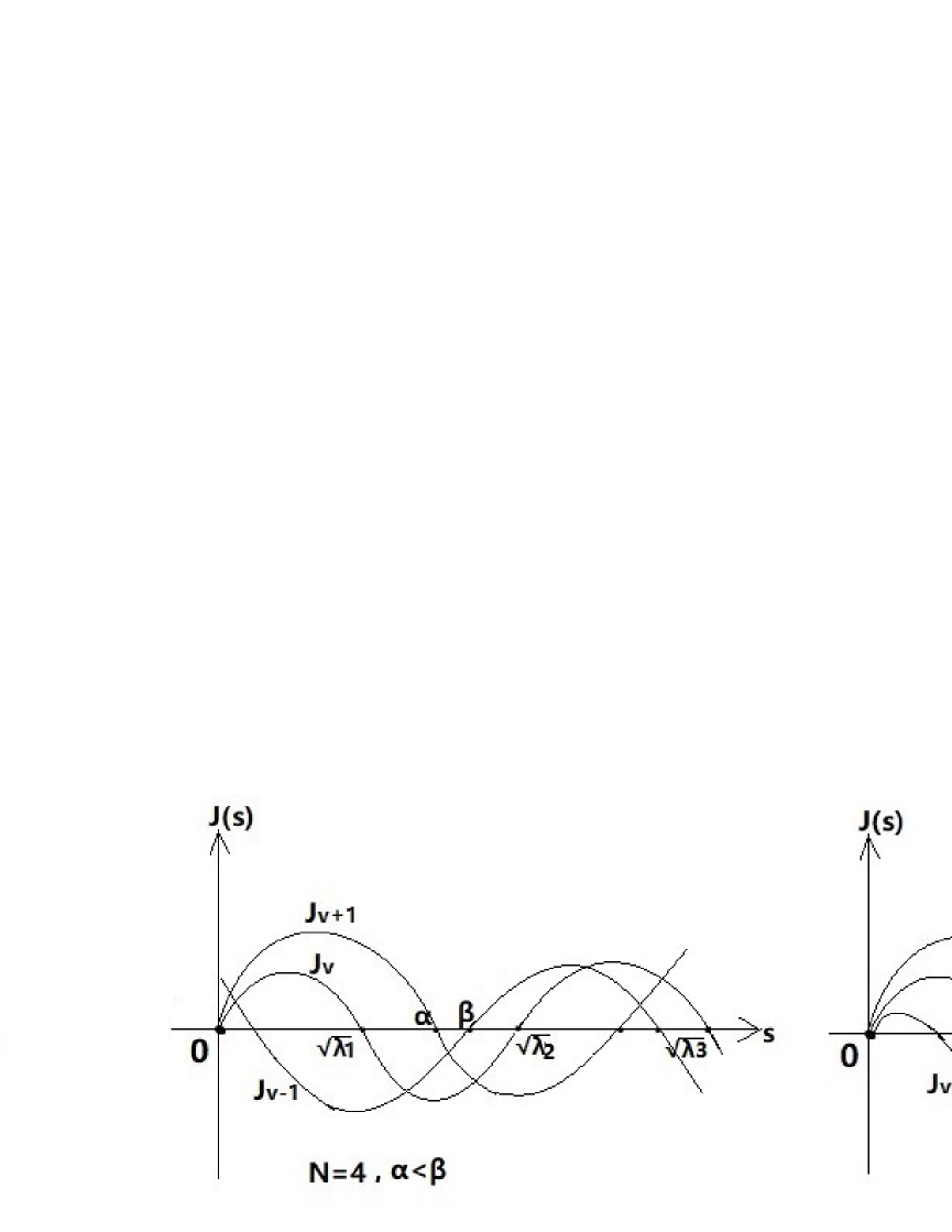
Figure 1: The profile of $J(s)$ for $N\geq 4$.

For $s\in\left(\alpha,\beta\right)$, we have that $J_{\nu-1}(s)J_{\nu+1}(s)>0$. Thus we have that

$$-2J_{\nu-1}(s)J_{\nu+1}(s)<0$$ (3.2)

for $s\in\left(\alpha,\beta\right)$. From the argument of [9, Proposition 3.2], we have known that inequality (3.2) is equivalent to

$$2J_{\nu}(s)sJ_{\nu}^{\prime}(s)>sJ_{\nu-1}^{\prime}(s)J_{\nu+1}(s)+J_{\nu-1}(s)sJ_{\nu+1}^{\prime}(s).$$

That is to say that

$$\left(J_{\nu}^{2}-J_{\nu-1}J_{\nu+1}\right)^{\prime}(s)>0.$$

So $J_{\nu}^{2}(s)-J_{\nu-1}(s)J_{\nu+1}(s)$ is strictly increasing in $\left(\alpha,\beta\right)$.Then, as that of [9, Proposition 3.2], we obtain that $h^{\prime}(s)>0$ for $s\in\left(\sqrt{\lambda_{1}},\sqrt{\lambda_{2}}\right)$. So, in view of (3.1), we conclude that $\sigma^{\prime}(T)>0$ for $T\in\left(T_{1},T_{2}\right)$ and $N\geq 4$.

We now consider the case $N=2$. In this case, $\nu=0$ and $J_{-1}(s)=-J_{1}(s)$. The profile of $J(s)$ is as following Figure 2.

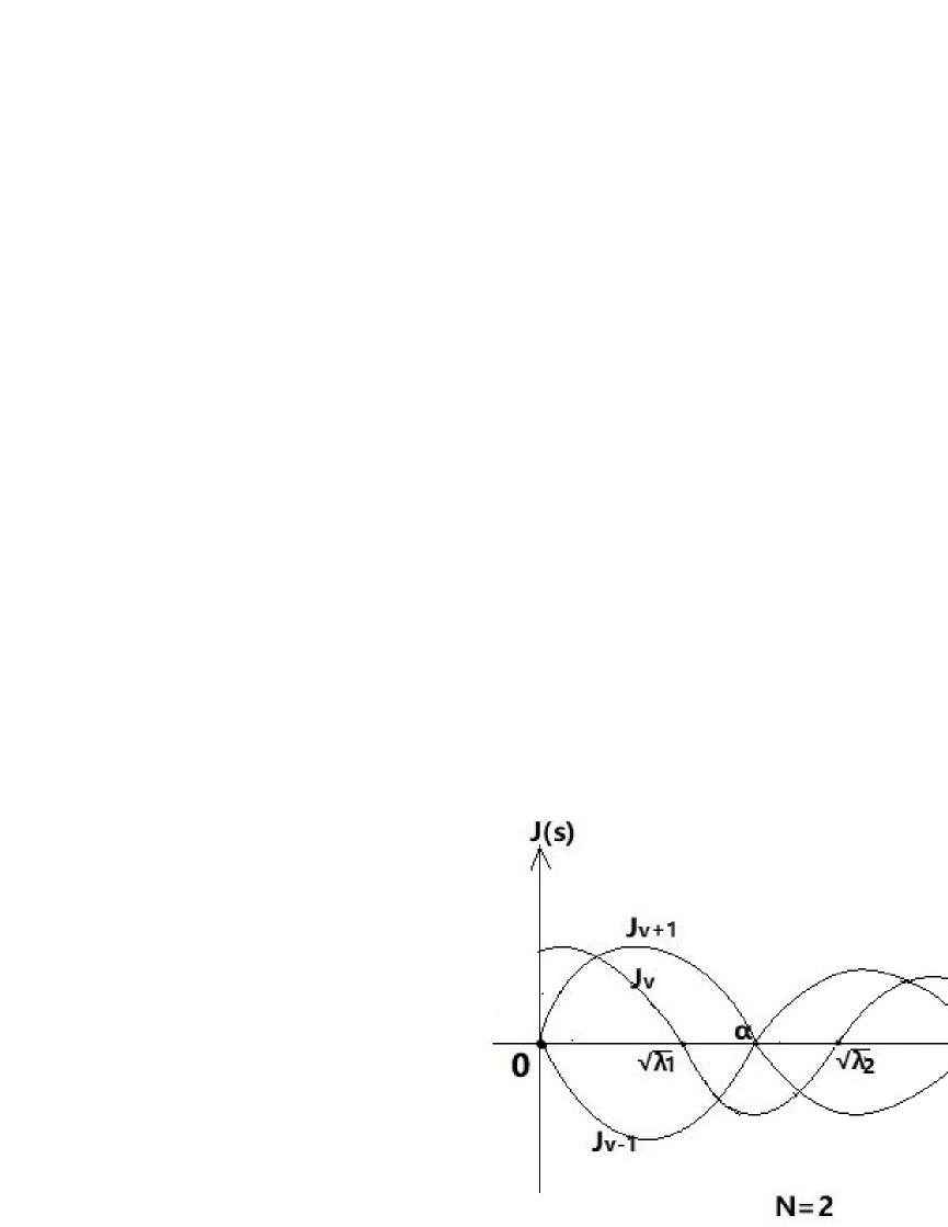
Figure 2: The profile of $J(s)$ for $N=2$.

Thus $J_{\nu-1}(s)J_{\nu+1}(s)=-J_{1}^{2}(s)\leq 0$ and we have that $J_{\nu}^{2}(s)-J_{\nu-1}(s)J_{\nu+1}(s)>0$ in $\left(\sqrt{\lambda_{1}},\sqrt{\lambda_{2}}\right)$. We still have that $h^{\prime}(s)>0$ for $s\in\left(\sqrt{\lambda_{1}},\sqrt{\lambda_{2}}\right)$, which implies that $\sigma^{\prime}(T)>0$ for $T\in\left(T_{1},T_{2}\right)$.

We now study the case of $N=3$. In this case, $\nu=1/2$, $\sqrt{\lambda_{1}}=\pi$ and $\sqrt{\lambda_{2}}=2\pi$ due to (2.3) and (2.2). From (2.2) we see that $J_{-1/2}(s)$ is positive in $\left(0,\pi/2\right)$, the first and second positive zeros are $\pi/2$ and $3\pi/2$, respectively. Define

$$\alpha=\min\left\{\frac{3\pi}{2},j_{\frac{3}{2},1}\right\},\,\,\beta=\max\left\{\frac{3\pi}{2},j_{\frac{3}{2},1}\right\}.$$

We note that $J_{-1/2}(s)$ and $J_{3/2}(s)$ have opposite signs in $\left(\sqrt{\lambda_{1}},\alpha\right)\cup\left(\beta,\sqrt{\lambda_{2}}\right)$. So, $h^{\prime}(s)>0$ for $s\in\left(\sqrt{\lambda_{1}},\alpha\right)\cup\left(\beta,\sqrt{\lambda_{2}}\right)$. If $\alpha=\beta$, we have that $J_{\nu}(\alpha)<0$ and $J_{\nu-1}(\alpha)J_{\nu+1}(\alpha)=0$. It follows that $J_{\nu}^{2}(\alpha)-J_{\nu-1}(\alpha)J_{\nu+1}(\alpha)>0$. So, $h^{\prime}(\alpha)>0$. When $\alpha<\beta$, The profile of $J(s)$ is as following Figure 3.

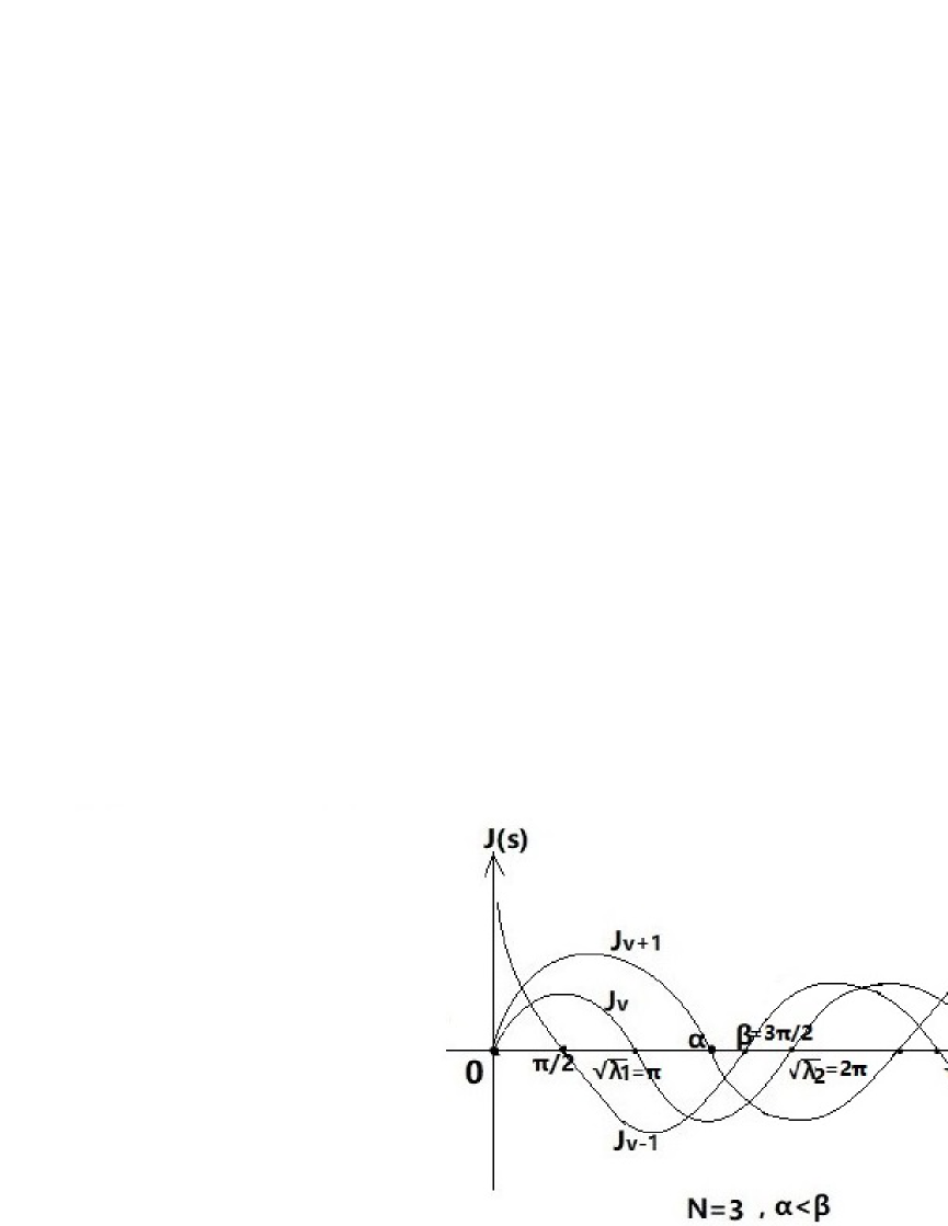
Figure 3: The profile of $J(s)$ for $N=3$.

Reasoning as in the case of $N\geq 4$, we have that $J_{\frac{1}{2}}^{2}(s)-J_{-\frac{1}{2}}(s)J_{\frac{3}{2}}(s)$ is strictly increasing in $\left(\alpha,\beta\right)$. Since $J_{-\frac{1}{2}}(\alpha)J_{\frac{3}{2}}(\alpha)=0$ and $J_{\frac{1}{2}}(\alpha)<0$, we have that $J_{\frac{1}{2}}^{2}(\alpha)-J_{-\frac{1}{2}}(\alpha)J_{\frac{3}{2}}(\alpha)>0$. Thus we obtain that

$$J_{\frac{1}{2}}^{2}(s)-J_{-\frac{1}{2}}(s)J_{\frac{3}{2}}(s)>0$$

for $s\in\left[\alpha,\beta\right]$. It follows that $h^{\prime}(s)>0$ for $s\in\left[\alpha,\beta\right]$. Therefore, we obtain that $h^{\prime}(s)>0$ for $s\in\left(\sqrt{\lambda_{1}},\sqrt{\lambda_{2}}\right)$ for $N=3$, which again indicates that $\sigma^{\prime}(T)>0$ for $T\in\left(T_{1},T_{2}\right)$.

As $T\in\left(T_{2},T_{3}\right)$, the profiles of Bessel functions are also shown in Figure 1–Figure 3 for $N\geq 2$. Repeating the above progress with slight changes, we obtain that $\sigma^{\prime}(T)>0$. Similarly, we can obtain that $\sigma^{\prime}(T)>0$ for $T\in\left(T_{i},T_{i+1}\right)$ for every $i\in\{2,\ldots,k-1\}$ with $T_{k}=+\infty$. Thus the proof is finished. ∎

From the argument of Proposition 3.2 we fact obtain the following convexity type inequality for the Bessel functions of the first kind

$$J_{\nu}^{2}(s)>J_{\nu-1}(s)J_{\nu+1}(s)$$

for all $s\in\left(0,+\infty\right)\setminus\left\{j_{\nu,1},j_{\nu,2},\cdots\right\}$, which extends the range $\left(0,j_{\nu,1}\right)$ obtained in [9, Claim A.1].

From Proposition 3.2 we conclude that $\sigma(T)$ has exactly $k$ zeros $T_{i,*}$ with $i\in\{1,\ldots,k\}$ such that

$$T_{i,*}\in\left(T_{i-1},T_{i}\right).$$

When $k$ is an even number we have that $\sigma^{\prime}\left(T_{i,*}\right)>0$, however, if $k$ is an odd number we have that $\sigma^{\prime}\left(T_{i,*}\right)<0$ as in the following figure 4. It should be pointed out that the above nondegeneracy of the zeros to $\sigma(T)$ is the key to verify the transversality condition in the famous Crandall-Rabinowitz Bifurcation Theorem.

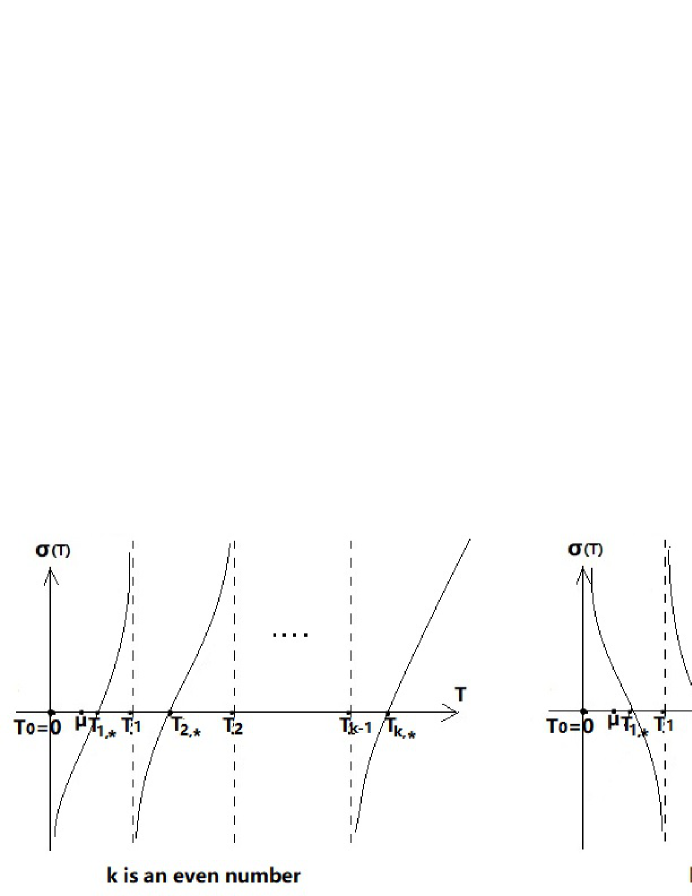
Figure 4: The profile of $\sigma(T)$.

We further obtain the following result.

Proposition 3.3. The kernel space of $D_{v}F\left(T_{1,*},0\right)$ is just $V_{1}$, where $V_{1}$ is the space spanned by the function $\cos(t)$. Moreover, for each $i\in\{2,\ldots,k\}$ and every $j\in\{1,\ldots,i-1\}$, if $T_{i,*}\neq lT_{j,*}$ for any $l\in\mathbb{N}$ with $l\geq 2$, the kernel space of $D_{v}F\left(T_{i,*},0\right)$ is still $V_{1}$. While, for each $i\in\{2,\ldots,k\}$, if there exist $m$ elements of $\{1,\ldots,i-1\}$ with $m\leq i-1$, which are denoted by $j_{n}$ with $n\in\{1,\ldots,m\}$, such that $T_{i,*}=l_{j_{n}}T_{j_{n},*}$ for some $l_{j_{n}}\in\mathbb{N}$ with $l_{j_{n}}\geq 2$ and $n\in\{1,\ldots,m\}$, the kernel space of $D_{v}F\left(T_{i,*},0\right)$ is just $\left(\cup_{n=1}^{m}V_{l_{j_{n}}}\right)\cup V_{1}$.

Proof. Without loss of generality, we only prove the case of $k$ being even. Clearly, $V_{1}$ is contained in the kernel space of $D_{v}F\left(T_{i,*},0\right)$ for every $i\in\{1,\ldots,k\}$. Note that

$$\sigma_{m}(T)=\sigma\left(\frac{T}{m}\right)$$

for all $m\in\mathbb{N}$. So $\sigma_{m}(T)$ has exactly one zero $mT_{i,*}$ in $\left(mT_{i-1},mT_{i}\right)$. Since $\sigma\left(T_{1,*}/j\right)<0$ with any $j\geq 2$, $V_{j}$ is not the kernel $D_{v}F\left(T_{1,*},0\right)$. Thus, the kernel space of $D_{v}F\left(T_{1,*},0\right)$ is just $V_{1}$.

For each $i\in\{2,\ldots,k\}$, if $T_{i,*}\neq lT_{j,*}$ for every $j\in\{1,\ldots,i-1\}$ and any $l\in\mathbb{N}$ with $l\geq 2$, $\sigma\left(T_{i,*}/l\right)\neq 0$. So $V_{l}$ is not the kernel $D_{v}F\left(T_{i,*},0\right)$ for any $l\geq 2$. Therefore, the kernel space of $D_{v}F\left(T_{i,*},0\right)$ is still $V_{1}$.

For each $i\in\{2,\ldots,k\}$, if there exist $m$ elements of $\{1,\ldots,i-1\}$ with $m\leq i-1$, which are denoted by $j_{n}$ with $n\in\{1,\ldots,m\}$, such that $T_{i,*}=l_{j_{n}}T_{j_{n},*}$ for some $l_{j_{n}}\in\mathbb{N}$ with $l_{j_{n}}\geq 2$ and $n\in\{1,\ldots,m\}$, we have that $\sigma\left(T_{i,*}/l_{j_{n}}\right)=\sigma\left(T_{j_{n},*}\right)=0$. So, for every $n\in\{1,\ldots,m\}$, $V_{l_{j_{n}}}$ is also contained in the kernel space of $D_{v}F\left(T_{i,*},0\right)$. Conversely, we claim that $V_{j}$ is not contained in the kernel $D_{v}F\left(T_{i,*},0\right)$ for any $j\not\in\left\{l_{j_{1}},\ldots,l_{j_{m}}\right\}$ with $j\geq 2$. Suppose, by contradiction, that $V_{j_{*}}$ is contained in the kernel $D_{v}F\left(T_{i,*},0\right)$ for some $j_{*}\not\in\left\{l_{j_{1}},\ldots,l_{j_{m}}\right\}$ with $j_{*}\geq 2$. Then we derive that $\sigma\left(T_{i,*}/j_{*}\right)=0$. This implies that $j_{*}\in\left\{l_{j_{1}},\ldots,l_{j_{m}}\right\}$, which is a contradiction. Therefore, the kernel space of $D_{v}F\left(T_{i,*},0\right)$ is just $\left(\cup_{n=1}^{m}V_{l_{j_{n}}}\right)\cup V_{1}$. ∎

From the conclusions of Proposition 3.3 we see that, for each $i\in\{2,\ldots,k\}$ and every $j\in\{1,\ldots,i-1\}$, if $T_{i,*}$ is not an integer multiple of $T_{j,*}$, the kernel space of $D_{v}F\left(T_{i,*},0\right)$ is one-dimensional. While, if $T_{i,*}$ is an integer multiple of some $T_{j,*}$ with $j\in\{1,\ldots,i-1\}$, the kernel space of $D_{v}F\left(T_{i,*},0\right)$ is multidimensional with the dimension less than $i$.

4 Proofs of Theorem 1.1–1.2

In this section, we will finish the main theorems by implementing bifurcation techniques. Based on arguments above, the Fredholm property and degeneracy of the linearized operator $F_{v}(0,T)$ are clear and the position of bifurcation points are shown in Figure 4. Thus it is standard as in [9, Section 4] to check corresponding conditions in Crandall-Rabinowitz type bifurcation theorem. Here we make up all details of this process for the convenience of readers. Now we first prove Theorem 1.1 by verifying the hypotheses of celebrated Crandall-Rabinowitz local bifurcation theorem [8].

Proof of Theorem 1.1. By Proposition 3.3, the kernel of the linearized operator $D_{v}F\left(0,T_{1,*}\right)$ is one-dimensional and is spanned by the function $\cos(t)$. As that of [25, Proposition 3.2] we can show that $D_{v}F\left(0,T_{1,*}\right)$ is a formally self-adjoint, first order elliptic operator. It follows that $D_{v}F\left(0,T_{1,*}\right)$ has closed range. Therefore, $D_{v}F\left(0,T_{1,*}\right)$ is a Fredholm operator of index zero (refer to [14]). So its codimension is equal to $1$. In view of Proposition 3.2, we obtain

$$D_{Tv}F\left(0,T_{1,*}\right)\cos(t)=\sigma^{\prime}\left(T_{1,*}\right)\cos(t)\not\in\text{Im}\left(D_{v}F\left(0,T_{1,*}\right)\right).$$

Applying the Crandall-Rabinowitz local bifurcation theorem [8] to $F(v,T)=0$, we obtain that there exist an open interval $I=\left(-\varepsilon,\varepsilon\right)$ and continuous functions $T:I\rightarrow\mathbb{R}$ and $w:I\rightarrow\text{Im}\left(D_{v}F\left(0,T_{1,*}\right)\right)$ such that $T(0)=T_{1,*}$, $w(0)=0$ and $F(s\cos(t)+sw(s),T(s))=0$ for $s\in I$ and $F^{-1}\{0\}$ near $\left(0,T_{1,*}\right)$ consists precisely of the curves $v=0$ and $\Gamma=\left\{(v(s),T(s)):s\in I\right\}$. Therefore, for each $s\in(-\varepsilon,\varepsilon)$, problem (1.3) has a $T(s)$-periodic solution $u\in\mathcal{C}^{2,\alpha}\left(\Omega_{s}\right)$ with the expected sign-changing property on the modified cylinder

$$\Omega_{s}=\left\{(x,t)\in\mathbb{R}^{N}\times\mathbb{R}:|x|<1+s\cos\left(\frac{2\pi}{T(s)}t\right)+sw(s)\left(\frac{2\pi}{T(s)}t\right)\right\},$$

which is the desired conclusion. ∎

Next we will establish Theorem 1.2 by verifying the hypotheses of Crandall-Rabinowitz local bifurcation theorem [9, Proposition 4.2] with high kernel.

Proof of Theorem 1.2. For each $i\in\{2,\ldots,k\}$ and every $j\in\{1,\ldots,i-1\}$, if $T_{i,*}\neq lT_{j,*}$ for any $l\in\mathbb{N}$ with $l\geq 2$, the kernel space of $D_{v}F\left(T_{i,*},0\right)$ is $V_{1}$. Then, in view of $\sigma^{\prime}\left(T_{i,*}\right)\neq 0$, repeating the argument as that of Theorem 1.1 we obtain the desired conclusion.

For each $i\in\{2,\ldots,k\}$, if there exist $m$ elements of $\{1,\ldots,i-1\}$ with $m\leq i-1$, which are denoted by $j_{n}$ with $n\in\{1,\ldots,m\}$, such that $T_{i,*}=l_{j_{n}}T_{j_{n},*}$ for some $l_{j_{n}}\in\mathbb{N}$ with $l_{j_{n}}\geq 2$ and $n\in\{1,\ldots,m\}$, it follows from Proposition 3.3 that the kernel space of $D_{v}F\left(T_{i,*},0\right)$ is just $\left(\cup_{n=1}^{m}V_{l_{j_{n}}}\right)\cup V_{1}$.

Reasoning as that of Theorem 1.1, $D_{v}F\left(0,T_{i,*}\right)$ is a formally self-adjoint, first order elliptic operator and has closed range. So $D_{v}F\left(0,T_{i,*}\right)$ is also a Fredholm operator of index zero (refer to [14]) with its codimension $m+1$. Since $\sigma^{\prime}\left(T_{i,*}\right)\neq 0$, we obtain

$$D_{Tv}F\left(0,T_{i,*}\right)\cos(t)=\sigma^{\prime}\left(T_{i,*}\right)\cos(t)\not\in\text{Im}\left(D_{v}F\left(0,T_{i,*}\right)\right).$$

Furthermore, since $\sigma^{\prime}\left(T_{j_{n},*}\right)\neq 0$, we obtain

$$D_{Tv}F\left(0,T_{i,*}\right)\cos\left(l_{j_{n}}t\right)=\frac{1}{l_{j_{n}}}\sigma^{\prime}\left(\frac{T_{i,*}}{l_{j_{n}}}\right)\cos\left(l_{j_{n}}t\right)=\frac{1}{l_{j_{n}}}\sigma^{\prime}\left(T_{j_{n},*}\right)\cos\left(l_{j_{n}}t\right)\not\in\text{Im}\left(D_{v}F\left(0,T_{i,*}\right)\right).$$

By applying [9, Proposition 4.2] to $F(v,T)=0$, we obtain that there exist an open interval $I=\left(-\varepsilon,\varepsilon\right)$ and continuous functions $T:I\rightarrow\mathbb{R}$, $w:I\rightarrow\text{Im}\left(D_{v}F\left(0,T_{i,*}\right)\right)$ such that $T(0)=T_{i,*}$, $w(0)=0$ and $F\left(s\left(\beta\cos(t)+\sum_{n=1}^{m}\gamma_{n}\cos\left(l_{j_{n}}t\right)\right)+sw(s),T(s)\right)=0$ for $s\in I$ with $\beta^{2}+\sum_{n=1}^{m}\gamma_{n}^{2}=1$ and $F^{-1}\{0\}$ near $\left(0,T_{i,*}\right)$ consists precisely of the curves $v=0$ and $\Gamma=\left\{(v(s),T(s)):s\in I\right\}$. Therefore, for each $s\in(-\varepsilon,\varepsilon)$, problem (1.3) has a $T(s)$-periodic solution $u\in\mathcal{C}^{2,\alpha}\left(\Omega_{s}\right)$ with the expected sign-changing property on the modified cylinder

$$\Omega_{s}=\left\{(x,t):|x|<1+s\left(\beta\cos\left(\frac{2\pi}{T(s)}t\right)+\sum_{n=1}^{m}\gamma_{n}\cos\left(\frac{2l_{j_{n}}\pi}{T(s)}t\right)\right)+sw(s)\left(\frac{2\pi}{T(s)}t\right)\right\},$$

as desired.∎

5 The one-dimensional case

For $N=1$, we have that

$$\lambda_{k}=\frac{(2k-1)^{2}\pi^{2}}{4}$$ (5.1)

and

$$\phi_{k}=\frac{1}{\sqrt{2\pi}}\cos\left(\frac{(2k-1)\pi}{2}r\right).$$

So we have that

$$\phi_{k}^{\prime}(1)=(-1)^{k}\frac{(2k-1)\sqrt{2\pi}}{4}\,\,\,\text{and}\,\,\,\phi_{k}^{\prime\prime}(1)=0.$$

It follows that

$$\sigma(T)=c^{\prime}(1)+\phi_{k}^{\prime\prime}(1)=c^{\prime}(1),$$

$c$ is the continuous solution on $[0,1]$ of

$$\left(\partial_{r}^{2}+\lambda_{k}\right)c-\left(\frac{2\pi}{T}\right)^{2}c=0$$ (5.2)

with $c(1)=-\phi_{k}^{\prime}(1)$ and $c^{\prime}(0)=0$. Proposition 2.2 implies $\sigma(T)$ is analytic when $T\neq T_{i}$ for any $i\in\{1,\ldots,k-1\}$. Based on (5.1), it is easy to deduce that $T_{i}=4/\sqrt{(2k-1)^{2}-(2i-1)^{2}}$ for $N=1$.

Lemma 5.1. For each $i\in\{1,\ldots,k\}$, the function $\sigma:\left(T_{i-1},T_{i}\right)\rightarrow\mathbb{R}$ has exactly one zero $T_{i,*}$ such that $\sigma^{\prime}\left(T_{i,*}\right)\neq 0$. In particular, $T_{1,*}=4/(2k-1)$ and $T_{i,*}=4/\sqrt{(2k-1)^{2}-4(i-1)^{2}}$ for each $i\in\{2,\ldots,k\}$, $\sigma^{\prime}\left(T_{i,*}\right)>0$ if $k$ is even and $\sigma^{\prime}\left(T_{i,*}\right)<0$ if $k$ is odd. Furthermore, when $k$ is even, for each $i\in\{1,\ldots,k-1\}$, the $\sigma(T)$ satisfies $\lim_{T\rightarrow 0^{+}}\sigma(T)=-\infty$, $\lim_{T\rightarrow T_{i}^{-}}\sigma(T)=+\infty$, $\lim_{T\rightarrow T_{i}^{+}}\sigma(T)=-\infty$ and $\lim_{T\rightarrow+\infty}\sigma(T)=+\infty$. While, when $k$ is odd, for each $i\in\{1,\ldots,k-1\}$, the $\sigma(T)$ satisfies $\lim_{T\rightarrow 0^{+}}\sigma(T)=+\infty$, $\lim_{T\rightarrow T_{i}^{-}}\sigma(T)=-\infty$, $\lim_{T\rightarrow T_{i}^{+}}\sigma(T)=+\infty$ and $\lim_{T\rightarrow+\infty}\sigma(T)=-\infty$.

Proof. Let

$$\alpha(T)=\frac{(2k-1)^{2}\pi^{2}}{4}-\left(\frac{2\pi}{T}\right)^{2}.$$

Then we have that

$$\alpha\left(\frac{4}{2k-1}\right)=0,$$

that is to say $\mu=4/(2k-1)$. By the Euler undetermined exponential function method, the characteristic equation of (5.2) is $\xi^{2}+\alpha=0$. Then the characteristic roots are: $\pm\sqrt{-\alpha}$ when $\alpha<0$; $\pm i\sqrt{\alpha}$ if $\alpha>0$; $0$ for $\alpha=0$. Combining with boundary conditions, we obtain that the solution of (5.2) is

$$c(r)=\left\{\begin{array}[]{ll}(-1)^{k-1}\frac{(2k-1)\sqrt{2\pi}}{4}\frac{\cosh\left(\sqrt{-\alpha(T)}r\right)}{\cosh\left(\sqrt{-\alpha(T)}\right)}&\text{if}\,\,\alpha<0,\\ (-1)^{k-1}\frac{(2k-1)\sqrt{2\pi}}{4}&\text{if}\,\,\alpha=0,\\ (-1)^{k-1}\frac{(2k-1)\sqrt{2\pi}}{4}\frac{\cos\left(\sqrt{\alpha(T)}r\right)}{\cos\left(\sqrt{\alpha(T)}\right)}&\text{if}\,\,\alpha>0.\end{array}\right.$$

Further, we have that

$$c(r)=\left\{\begin{array}[]{ll}(-1)^{k-1}\frac{(2k-1)\sqrt{2\pi}}{4}\frac{\cosh\left(\sqrt{-\alpha(T)}r\right)}{\cosh\left(\sqrt{-\alpha(T)}\right)}&\text{if}\,\,T\in\left(0,\frac{4}{2k-1}\right),\\ (-1)^{k-1}\frac{(2k-1)\sqrt{2\pi}}{4}&\text{if}\,\,T=\frac{4}{2k-1},\\ (-1)^{k-1}\frac{(2k-1)\sqrt{2\pi}}{4}\frac{\cos\left(\sqrt{\alpha(T)}r\right)}{\cos\left(\sqrt{\alpha(T)}\right)}&\text{if}\,\,T\in\left(\frac{4}{2k-1},+\infty\right)\setminus\left\{T_{1},\ldots,T_{k-1}\right\}.\end{array}\right.$$

So we get that

$$\sigma(T)=\left\{\begin{array}[]{ll}(-1)^{k-1}\frac{(2k-1)\sqrt{2\pi}}{4}\sqrt{-\alpha(T)}\tanh\left(\sqrt{-\alpha(T)}\right)&\text{if}\,\,T\in\left(0,\frac{4}{2k-1}\right),\\ 0&\text{if}\,\,T=\frac{4}{2k-1},\\ (-1)^{k}\frac{(2k-1)\sqrt{2\pi}}{4}\sqrt{\alpha(T)}\tan\left(\sqrt{\alpha(T)}\right)&\text{if}\,\,T\in\left(\frac{4}{2k-1},+\infty\right)\setminus\left\{T_{1},\ldots,T_{k-1}\right\}.\end{array}\right.$$

It follows that

$$(-1)^{k}\sigma(T)<0\,\,\,\text{for}\,\,\,T<\frac{4}{2k-1}$$

and

$$(-1)^{k}\sigma(T)>0\,\,\,\text{for}\,\,\,T\in\left(\frac{4}{2k-1},T_{1}\right).$$

That is to see $4/(2k-1):=T_{1,*}$ is the unique zero of $\sigma(T)$ in $\left(0,T_{1}\right)$.

Since $\lim_{T\rightarrow 0^{+}}\alpha(T)=-\infty$, when $k$ is even, $\sigma(T)$ satisfies $\lim_{T\rightarrow 0^{+}}\sigma(T)=-\infty$. While, when $k$ is odd, $\sigma(T)$ satisfies $\lim_{T\rightarrow 0^{+}}\sigma(T)=+\infty$. Further, since $\lim_{T\rightarrow+\infty}\alpha(T)=\lambda_{k}=(2k-1)^{2}\pi^{2}/4$, we have that $\lim_{T\rightarrow+\infty}\sigma(T)=+\infty$ (or $\lim_{T\rightarrow+\infty}\sigma(T)=-\infty$) if $k$ is even (or odd). Noting that

$$\alpha\left(T_{i}\right)=\lambda_{i}=\frac{(2i-1)^{2}\pi^{2}}{4}$$

for each $i\in\{1,\ldots,k-1\}$, we see that $\sigma(T)$ is singular at $T=T_{i}$. Therefore, when $k$ is even, for each $i\in\{1,\ldots,k-1\}$, $\sigma(T)$ satisfies $\lim_{T\rightarrow T_{i}^{-}}\sigma(T)=+\infty$ and $\lim_{T\rightarrow T_{i}^{+}}\sigma(T)=-\infty$. While, when $k$ is odd, for each $i\in\{1,\ldots,k-1\}$, $\sigma(T)$ satisfies $\lim_{T\rightarrow T_{i}^{-}}\sigma(T)=-\infty$ and $\lim_{T\rightarrow T_{i}^{+}}\sigma(T)=+\infty$.

The above asymptotic behavior implies that the function $\sigma:\left(T_{i-1},T_{i}\right)\rightarrow\mathbb{R}$ for $i\in\{1,\ldots,k\}$ has at least one zero. In particular, $\sigma(T)$ has exactly one zero in $\left(0,T_{1}\right)$. To get further information of these zeros, we compute the derivative of $\sigma(T)$ as follows

$$\sigma^{\prime}(T)=(-1)^{k}\frac{(2k-1)\sqrt{2\pi}}{8\sqrt{-\alpha(T)}}\alpha^{\prime}(T)\left(\tanh\left(\sqrt{-\alpha(T)}\right)+\frac{\sqrt{-\alpha(T)}}{\cosh^{2}\left(\sqrt{-\alpha(T)}\right)}\right)$$ (5.3)

for $T\in\left(0,T_{1,*}\right)$, and

$$\sigma^{\prime}(T)=(-1)^{k}\frac{(2k-1)\sqrt{2\pi}}{8\sqrt{\alpha(T)}}\alpha^{\prime}(T)\left(\tan\left(\sqrt{\alpha(T)}\right)+\sqrt{\alpha(T)}\sec^{2}\left(\sqrt{\alpha(T)}\right)\right)$$ (5.4)

for $T\in\left(T_{1,*},+\infty\right)\setminus\left\{T_{1},\ldots,T_{k-1}\right\}$. It follows (5.3) that $(-1)^{k}\sigma^{\prime}(T)>0$ for $T\in\left(0,T_{1,*}\right)$.

Now let’s show $(-1)^{k}\sigma^{\prime}\left(T_{1,*}\right)>0$. From (5.3), it is obvious that the left derivative of $\sigma$ at $T=T_{1,*}=4/(2k-1)$ is

$$\lim_{T\rightarrow\left(\frac{4}{2k-1}\right)^{-}}(-1)^{k}\frac{(2k-1)\sqrt{2\pi}}{8\sqrt{-\alpha(T)}}\alpha^{\prime}(T)\left(\tanh\left(\sqrt{-\alpha(T)}\right)+\frac{\sqrt{-\alpha(T)}}{\cosh^{2}\left(\sqrt{-\alpha(T)}\right)}\right)$$

$$= \frac{(-1)^{k}(2k-1)^{4}\pi^{2}\sqrt{2\pi}}{64}\lim_{T\rightarrow\left(\frac{4}{2k-1}\right)^{-}}\left(\frac{\tanh\left(\sqrt{-\alpha(T)}\right)}{\sqrt{-\alpha(T)}}+\frac{1}{\cosh^{2}\left(\sqrt{-\alpha(T)}\right)}\right),$$

where we use the fact of $\alpha^{\prime}\left(4/(2k-1)\right)=(2k-1)^{3}\pi^{2}/8$. By the L’Hospital rule we know that

$$\lim_{x\rightarrow 0}\frac{\tanh(x)}{x}=\lim_{x\rightarrow 0}\frac{1}{\cosh^{2}(x)}=1.$$

So we have that

$$\lim_{T\rightarrow\left(\frac{4}{2k-1}\right)^{-}}\left(\frac{\tanh\left(\sqrt{-\alpha(T)}\right)}{\sqrt{-\alpha(T)}}+\frac{1}{\cosh^{2}\left(\sqrt{-\alpha(T)}\right)}\right)=2$$

due to $\lim_{T\rightarrow\left(\frac{4}{2k-1}\right)^{-}}\alpha(T)=0$. Therefore, the left derivative of $\sigma$ at $T=4/(2k-1)$ is

$$\sigma^{\prime}\left(\frac{4}{2k-1}-0\right)=\frac{(-1)^{k}(2k-1)^{4}\pi^{2}\sqrt{2\pi}}{32}.$$

Further, the analyticity of $\sigma(T)$ implies that $(-1)^{k}\sigma^{\prime}\left(T_{1,*}\right)>0$.

We now consider the case $T\in\left(T_{1,*},T_{1}\right)$. In this case, we find that

$$0<\alpha(T)<\lambda_{1}=\frac{\pi^{2}}{4}.$$

So we have that $\tan\sqrt{\alpha(T)}>0$. It follows from (5.4) that $(-1)^{k}\sigma^{\prime}(T)>0$ for $T\in\left(T_{1,*},T_{1}\right)$.

Next we consider the case $T\in\left(T_{i-1},T_{i}\right)$ for any $i\in\{2,\ldots,k-1\}$. Then we find that

$$\frac{(2i-3)^{2}\pi^{2}}{4}=\lambda_{i-1}<\alpha(T)<\lambda_{i}=\frac{(2i-1)^{2}\pi^{2}}{4}.$$

We consider the following function

$$h(x)=\frac{\tan(x)}{x}+\frac{1}{\cos^{2}(x)},\,\,x\in\left(\frac{(2i-3)\pi}{2},\frac{(2i-1)\pi}{2}\right).$$

Setting $\tan x=y$, we get that

$$h(x)=1+y^{2}+\frac{y}{x}:=\widetilde{h}(y).$$

Then we see that the discriminant is negative due to the range of $x$. Thus, one has that $h(x)=\widetilde{h}(y)>0$ for given interval which implies that $(-1)^{k}\sigma^{\prime}(T)>0$ for $T\in\left(T_{i-1},T_{i}\right)$. Therefore, we conclude that $(-1)^{k}\sigma^{\prime}(T)>0$ for $T\in\left(0,4/(2k-1)\right)\cup\left(4/(2k-1),+\infty\right)\setminus\left\{T_{1},\ldots,T_{k-1}\right\}$. Hence, for each $i\in\{2,\ldots,k\}$, $\sigma$ also has a unique zero in $\left(T_{i-1},T_{i}\right)$, which is denoted by $T_{i,*}$, such that $(-1)^{k}\sigma^{\prime}\left(T_{i,*}\right)>0$.

We can further give the exact values of $T_{i,*}$. For $T\in\left(T_{i-1},T_{i}\right)$ with $i\in\{2,\ldots,k\}$, we see that

$$\frac{(2i-3)^{2}\pi^{2}}{4}=\lambda_{i-1}<\alpha\left(T\right)<\lambda_{i}=\frac{(2i-1)^{2}\pi^{2}}{4}.$$

We find that $\sigma(T)=0$ if and only if $\sqrt{\alpha\left(T\right)}=(i-1)\pi$. It follows from the definition of $\alpha\left(T\right)$ that

$$T_{i,*}=\frac{4}{\sqrt{(2k-1)^{2}-4(i-1)^{2}}}$$

for any $k\in\mathbb{N}$ and each $i\in\{2,\ldots,k\}$. ∎

In view of Lemma 5.1, by using the classical Crandall-Rabinowitz local bifurcation theorem and the modified version with high kernel, the conclusions of Theorems 1.1–1.2 are all valid for $N=1$. It is worth noting that $\mu=T_{1,*}=4/(2k-1)$ at this time.

Remark 5.2. For $N=1$ and any given positive integer $k$, we find that the bifurcation points are $T_{i,*}=4/\sqrt{(2k-1)^{2}-4(i-1)^{2}}$ for $1\leq i\leq k$ with $i\in\mathbb{N}^{+}$. If there exist some positive integer $l\geq 2$ such that $T_{i,*}=lT_{j,*}$ by choosing some suitable $i,j\in[1,k]$ with $i,j\in\mathbb{N}^{+}$, then the case of multidimensional kernels would take place. In fact, there are a lot of choice for $(k,i,j,l)$ to ensure the case must occur by using the computer-aided calculation. For instance, here we list some choice in the following table.

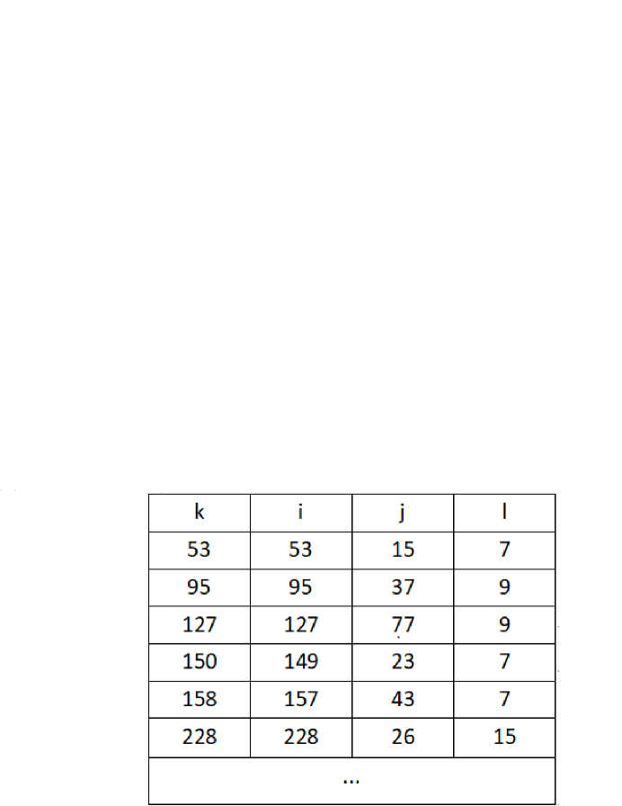
Figure 5: Some choice to ensure the occurrence of multidimensional kernels.

References

1. A. Aftalion and J. Busca, Symétrie radiale pour des problèmes elliptiques surdéterminés posés dans des domaines
extérieurs, C. R. Acad. Sci. Paris Sér. I Math. 324 (1997), 633–638.
2. A. Ambrosetti and A. Malchiodi,
Nonlinear analysis and semilinear elliptic problems, Cambridge Studies in Advanced Mathematics, vol. 104, Cambridge University Press, Cambridge, 2007.
3. C.A. Berenstein, An inverse spectral theorem and its relation to the Pompeiu problem, J. Anal. Math. 37 (1980), 128–144.
4. C.A. Berenstein and P.C. Yang, An overdetermined Neumann problem in the unit disk, Adv. Math. 44 (1982), 1–17.
5. C.A. Berenstein and P.C. Yang, An inverse Neumann problem, J. Reine Angew. Math. 382 (1987), 1–21.
6. H. Berestycki, L.A. Caffarelli and L. Nirenberg, Monotonicity for elliptic equations in unbounded Lipschitz domains,
Comm. Pure Appl. Math. 50 (1997), 1089–1111.
7. E.A. Coddington and N. Levinson, Theory of ordinary oifferential oquations, McGraw CHill, New York, 1955.
8. M.G. Crandall and P.H. Rabinowitz, Bifurcation from simple eigenvalues, J. Funct. Anal. 8 (1971), 321–340.
9. G. Dai and Y. Zhang, Sign-changing solution for an overdetermined elliptic problem on unbounded domain, J. Reine Angew. Math. (Crelle’s Journal), doi: 10.1515/crelle-2023-0059.
11. A. Farina and E. Valdinoci, Flattening results for elliptic PDEs in unbounded domains with applications to overdetermined problems, Arch. Ration. Mech. Anal. 195 (2010), 1025–1058.
12. D. Gilbarg and N.S. Trudinger, Elliptic Partial Differential Equations of Second Order, Springer-Verlag, Berlin, Heidelberg, 2001.
13. E.L. Ince, Ordinary differential equation, Dover Publication Inc., New York, 1927.
14. C.S. Kubrusly, Fredholm theory in Hilbert space-A concise introductory exposition, Bull. Belg. Math. Soc. Simon Stevin 15 (2008), 153–177.
15. I.A. Minlend, An overdetermined problem for sign-changing eigenfunctions in unbounded domains, arXiv:2203.15492v1.
16. I.A. Minlend, Overdetermined problems with sign-changing eigenfunctions in unbounded periodic domains, arXiv:2307.07784.
17. F.M. Olver, D.W. Lozier, R.F. Boisvert and C.W. Clark, NIST handbook of mathematical functions hardback
and CD-ROM, Cambridge university press, 2010.
18. P. Pucci and J. Serrin, The maximum principle, Progr. Nonlinear Differential Equations Appl., vol. 73, Birkhäuser
Verlag, Basel, 2007.
19. W. Reichel, Radial symmetry for elliptic boundary-value problems on exterior domains, Arch. Ration. Mech.
Anal. 137 (1997), 381–394.
20. A. Ros, D. Ruiz and P. Sicbaldi, A rigidity result for overdetermined elliptic problems in the
plane, Comm. Pure Appl. Math. 70 (2017), 1223–1252.
21. D. Ruiz, Nonsymmetric sign-changing solutions to overdetermined elliptic problems in bounded domains, arXiv:2211.14014v1.
22. D. Ruiz, P. Sicbaldi and J. Wu, Overdetermined elliptic problems in onduloid-type domains with general nonlinearities, J. Funct. Anal. 283 (2022), no. 12, Paper No. 109705, 26 pp.
23. F. Schlenk and P. Sicbaldi, Bifurcating extremal domains for the first eigenvalue of the Laplacian, Adv. Math. 229 (2012), 602–632.
24. J. Serrin, A symmetry problem in potential theory, Arch. Ration. Mech. Anal. 43 (1971), 304–318.
25. P. Sicbaldi, New extremal domains for the first eigenvalue of the Laplacian in flat tori, Calc. Var. Partial Differential
Equations 37 (2010), 329–344.
26. L.A. Shepp and J. B. Kruskal, Computerized tomography: the new medical -ray technology,
Amer. Math. Monthly 85 (1978), 420–439.
27. R. Temam, A non-linear eigenvalue problem: The shape at equilibrium of a confined plasma,
Arch. Rational Mech. Anal. 60 (1975), 51–73.
28. W. Walter, Ordinary Differential Equations, Springer, New York, 1998.