The $\mathfrak{S}_{k}$-circular limit of random tensor flattenings

Abstract

The tensor flattenings appear naturally in quantum information when one produces a density matrix by partially tracing the degrees of freedom of a pure quantum state. In this paper, we study the joint ^∗-distribution of the flattenings of large random tensors under mild assumptions, in the sense of free probability theory. We show the convergence toward an operator-valued circular system with amalgamation on permutation group algebras for which we describe the covariance structure. As an application we describe the law of large random density matrix of bosonic quantum states.

Primary 15B52, 46L54; Keywords: Free Probability, Large Random Matrices, Random Tensors, Quantum Information, Bosonic quantum states

1 Introduction and presentation of the problem

Let $F$ be an $N$-dimensional complex vector space given with a basis, and let $k\geq 1$ be a fixed integer. Thanks to the coordinates in this basis, we represent a tensor of order $2k$ on $F$ as a multi-indexed vector in $(\mathbb{C}^{N})^{\otimes 2k}$, such as

$$M_{N}=\big{(}m(i_{1},\ldots,i_{2k})\big{)}_{i_{1},\ldots,i_{2k}\in[N]}\in(\mathbb{C}^{N})^{\otimes 2k},$$

where $[N]:=\{1,\ldots,N\}$. Splitting the $k$ first and $k$ last indices, a tensor $M_{N}$ is canonically associated to a matrix of $\mathrm{M}_{N^{k}}(\mathbb{C})$ that represents the endomorphism of $(\mathbb{C}^{N})^{\otimes k}$

$$M_{N,id}:=\big{(}m(\mathbf{i},\mathbf{j})\big{)}_{\mathbf{i},\mathbf{j}\in[N]^{k}}\in\mathrm{End}\big{(}(\mathbb{C}^{N})^{\otimes k}\big{)}\cong\mathrm{M}_{N^{k}}(\mathbb{C}).$$

Furthermore, we can also represent a tensor differently by shuffling the role of the indices, producing different matrices here called “flattenings” and sometimes “matricization” or “unfolding” of the initial tensor. More precisely, let us denote by $\mathfrak{S}_{2k}$ the symmetric group of order $2k$, that is the group of bijections of $[2k]$.

Definition 1.1.

For any tensor $M_{N}\in(\mathbb{C}^{N})^{\otimes 2k}$ and any bijection $\sigma\in\mathfrak{S}_{2k}$, we define the element of $\mathrm{M}_{N^{k}}(\mathbb{C})\sim\mathrm{End}\big{(}(\mathbb{C}^{N})^{k}\big{)}$

$$M_{N,\sigma}:=\Big{(}M_{N}\big{(}i_{\sigma^{-1}(1)},\dots,i_{\sigma^{-1}(2k)}\big{)}\Big{)}_{(i_{1},\dots,i_{k}),(i_{k+1},\ldots,i_{2k})\in[N]^{k}},$$ (1.1)

that is called a flattening for short of $M_{N}$.

For $k=1$, there are 2 permutations: $\mathrm{id}$ and the transposition $(1,2)$, so there are 2 flattenings: the canonical one $M_{N,\mathrm{id}}$ and its transpose $M_{N,(1,2)}=(M_{N,\mathrm{id}})^{\top}$. For general order $k\geq 1$, there are up to $(2k)!$ different flattenings of a tensor.

We work under the following assumptions.

Hypothesis 1.2.

The tensor $M_{N}\in(\mathbb{C}^{N})^{\otimes 2k}$ has i.i.d. entries distributed as a centered complex random variable $m_{N}$ having finite moments of all orders (i.e. $\mathbb{E}\big{[}|m_{N}|^{\ell}\big{]}<\infty$ for all $\ell$). Moreover, the following limits exist

$$N^{k}\times\mathbb{E}\big{[}|m_{N}|^{2}\big{]}\underset{N\rightarrow\infty}{\longrightarrow}c>0, N^{k}\times\mathbb{E}\big{[}m_{N}^{2}\big{]}\underset{N\rightarrow\infty}{\longrightarrow}c^{\prime}\in\mathbb{C},$$ (1.2)

and for all non-negative integers $\ell_{1},\ell_{2}$ such that $\ell_{1}+\ell_{2}>2$

$$N^{k}\times\mathbb{E}\big{[}m_{N}^{\ell_{1}}\overline{m_{N}}^{\ell_{2}}\big{]} \underset{N\rightarrow\infty}{\longrightarrow} 0.$$ (1.3)

We call $(c,c^{\prime})$ the parameter of $M_{N}$.

Example 1.3.

In item 2, we use the notation $x\leadsto\nu$ to mean that a complex random variable $x$ is distributed according to a probability distribution $\nu$.

1. Let $M_{N}$ be sampled according to the complex Ginibre ensemble, i.e. the entries of $\sqrt{N}M_{N}$ are distributed according to the standard complex Gaussian distribution. Then $M_{N}$ satisfies Hypothesis 1.2 and its parameter is $(1,0)$. A real Ginibre ensemble also satisfies the hypothesis with parameter $(1,1)$.

2. Let $p_{N}\in]0,1],N\geq 1$ be a sequence of real numbers and let $\mu$ be the distribution of a complex random variable with no atom in 0, and with finite moments of all orders. We denote the probability measure

   $$\nu:=(1-p_{N})\delta_{0}+p_{N}\mu.$$ (1.4)

   If $\mu$ is a Dirac mass, we assume $p_{N}<1/2$. Let $M_{N}$ be a random tensor with i.i.d. entries distributed as $\sigma^{-2}_{N}(x-\alpha\,p_{N})$ with $x\leadsto\nu$, where for a variable $y\leadsto\mu$ we have set $\alpha=\mathbb{E}[y]$, $\beta^{2}=\mathbb{E}[|y|^{2}]$ and $\sigma_{N}=N^{k}p_{N}(\beta^{2}-|\alpha|^{2}p_{N})$. If $N^{k}p_{N}$ tends to infinity, then $M_{N}$ satisfies Hypothesis 1.2 and its parameter is $(\mathbb{E}[|y|^{2}],\mathbb{E}[y^{2}]\big{)}$ where $y\leadsto\mu$.

Remark 1.4.

A variable sampled from $\nu$ defined in (1.4) is distributed according to $\mu$ with probability $p_{N}$ and is equal to zero otherwise. We say that $\nu$ is a dilution of $\mu$. The entries of $M_{N}$ are normalized to be centered and in order to get the announced parameter. The sequence $p_{N}$ is allowed to converge to zero, provided the average number of entries different from the constant $\alpha p_{N}$ in each column of a flattenings of $M_{N}$ converges to infinity.

In this article, we consider the collection of all the flattenings of such a random tensor. We study the ^∗-distribution of this family in the sense of free probability (whose definition is recalled in Section 2). Under the above assumptions, we characterize the limit in simple terms thanks to operator-valued free probability theory, which is the non commutative analogue of conditional probability. Our main result stated in Theorem 2.15, establishes that the limit of the flattenings is an operator-valued circular collection.

This extends freeness results of a random matrix and its transpose, which is known for unitarily invariant random matrices that converge in ^∗-distribution [MP16], and more generally for ”asymptotically unitarily invariant matrices” in the sense of traffics [CDM16], which includes matrices with i.i.d. entries. It also In constrast with the results of these cited works, we show that in our more general setting freeness does not hold between all the flattenings. Other studies of random tensors in the context of free probability include the asymptotic freeness of a Wishart matrix and its partial transpose [PM20], asymptotic semicircularity for contracted Wigner-type tensors [AGV21]. Our result also generalizes [DLN20, Theorem 4.13] when we restrict our attention to square matrices.

Our motivation for this paper comes from quantum information theory. Recall first that the singular values of a matrix $A_{N}$ are the square roots of the eigenvalues of the positive semidefinite matrix $A_{N}A_{N}^{*}$. For a random matrix $A_{N}$, we call (averaged) empirical singular values distribution the probability measure $\mathbb{E}\big{[}\frac{1}{N}\sum_{i\in[N]}\delta_{s_{i}}\big{]}$, where $\delta_{s_{i}}$ denote the Dirac mass at the singular values $s_{i}$ of $A_{N}$. If $A_{N}$ is Hermitian, we call (averaged) empirical eigenvalues distribution the probability measure $\mathbb{E}\big{[}\frac{1}{N}\sum_{i\in[N]}\delta_{\lambda_{i}}\big{]}$, where the $\lambda_{i}$’s are the eigenvalues of $A_{N}$. The symmetrized matrix

$$\sum_{\sigma,\sigma^{\prime}\in\mathfrak{S}_{2k}}M_{N,\sigma}M_{N,\sigma^{\prime}}$$ (1.5)

is, up to normalization, the density matrix associated to the partial trace over a bipartition of a random quantum states of bosons. Bosons are one of the two flavors (together with fermions) of undistiguinshable particles in nature. Their quantum states must be invariant under exchange of particles.
The typical properties of such random states have not been studied in much details in the mathematical literature despite the fact that in many contexts (e.g. condensed matter) they are much more natural states to consider. An attempt at studying a model that is close in spirit can be found here [DNT22].

In the present paper, we describe the spectrum of the marginals of (un-normalized) random bosonic states in order to bound their limiting geometric bipartite entanglement. In fact a consequence of our work is that the largest Schmidt coefficients of such states before normalization is asymptotically bounded from below by $2$. This Schmidt coefficient is a well known measure of bipartite entanglement which directly relates to geometric entanglement [WG03].
This is a first step in our work, as we plan to use the results of this paper to study the spectrum of the partial transpose of bosonic quantum states in the future. Indeed, we know from numerical simulations their spectrum is behaving very differently from the spectrum of the partial transpose of quantum states with no symmetry.
Moreover, we hope that this formalism could be used to study general permutational criteria of entanglement [HHH02] of which the partial transpose and the realignment criteria are well known special cases, as indeed the permutational criteria can be encoded through the action of $\mathfrak{S}_{2k}$ on density matrices.
Finally, though our work sheds no new light on this specific aspect, we want to point out the importance of flattenings of quantum states to study entanglement. In fact, the separability of quantum states is equivalent to the vanishing of all the $2\times 2$ minors of some of its flattenings, called contraction maps [Ott13].

Another motivation comes from data analysis, where information on a noisy data tensor is retrieved from the spectral properties of its flattenings for instance in the context of Multilinear Subspace Analysis (MSA) [GSMZW09]. Our work could give insight on the free independence properties of the flattenings of the noisy part of such data tensors. In particular, we allow the tensor to be diluted, i.e. to have a majority of zero entries which is a regime appearing in e.g. community detection [PZ21] or in MSA with (a lot of) missing values.
Finally, one of the most important recent use of flattenings of tensors is in the context of tensors PCA, where when they are used to initialize tensor powers algorithms drastically improve the detection threshold of this family of algorithms while having a better accuracy above the threshold. See [RM14] for a foundational work on this topic (see [RM14, section 3 and 6]).

To conclude this section, let us discuss in more detail a simple situation that our result solve. Let $M_{N}$ be a random tensor satisfying Hypothesis 1.2 with parameter $(c,c^{\prime})$. It is known that, for each $\sigma\in\mathfrak{S}_{2k}$, the empirical eigenvalues distribution of $M_{N,\sigma}M_{N,\sigma}^{*}$ converges to the Marčhenko-Pastur distribution $\mathrm{MP}_{c}=\mathrm{MP}_{c,1}$ of variance $c$ and shape parameter $\lambda=1$ (since the matrices we consider are square). We recall that the $\mathrm{MP}_{c,\lambda}$ distribution has the following form

$$\mathrm{MP}_{c,\lambda}=\max(1-\frac{1}{\lambda},0)\delta_{0}+\frac{\sqrt{(b-x)(x-a)}}{2\pi c\lambda x}\mathbbm{1}_{x\in(a,b)}\mathrm{d}x,$$

with $a=c(1-\sqrt{\lambda})^{2}$, $b=c(1+\sqrt{\lambda})^{2}$. As expressed earlier, in this work we consider the $\lambda=1$ case.

More generally, it is known in free probability that each flattening converges in non-commutative distribution to a so-called circular variable [MS17] (see next section for the definitions). Furthermore, when $c^{\prime}=0$ the transpose $M_{N,\sigma}^{\top}$ is also known from works of Mingo and Popa [MP16] as well as Cébron, Dahlqvist and the second named author of this paper [CDM16] to be asymptotically free from $M_{N,\sigma}$, so $S^{\pm}_{N,\sigma}=1/\sqrt{2}(M_{N,\sigma}\pm M_{N,\sigma}^{\top})$ converges to a circular variable with same variance. Therefore, the empirical eigenvalues distribution of $S^{\pm}_{N,\sigma}{S^{\pm}_{N,\sigma}}^{*}$ converges to a Marčhenko-Pastur distribution. Similarly the empirical eigenvalues distribution of $S^{\pm}_{N,\sigma}+{S^{\pm}_{N,\sigma}}^{*}$ converges to a semicircular distribution.

One can also check (see Section 4) that the limits of the matrices are decorrelated, that is $\mathbb{E}\big{[}\frac{1}{N}\mathrm{Tr}M_{N,\sigma}M_{N,\sigma^{\prime}}^{*}\big{]}\underset{N\rightarrow\infty}{\longrightarrow}0$ if $\sigma\neq\sigma^{\prime}$. Hence it is natural to wonder if the collection of all matrices $M_{N,\sigma}$ converges to free circular variables for $k\geq 2$. This is not true as shows the following consequence of our main result.

Corollary 1.5.

Let $k\geq 1$ be a fixed integer. Let $M_{N}$ be a random tensor satisfying Hypothesis 1.2 with parameter $(c,c^{\prime})$. We consider the three following random matrices

$$S_{1,N}=\frac{1}{\sqrt{(2k)!k!c}}\sum_{\sigma\in\mathfrak{S}_{2k}}M_{N,\sigma},\quad S_{2,N}=\frac{1}{\sqrt{(2k)!k!c}}\sum_{\sigma\in\mathfrak{S}_{2k}}\mathrm{sg}(\sigma)\,M_{N,\sigma},$$

$$S_{3,N}=\frac{1}{2\sqrt{(2k)!k!(c+\Re c^{\prime})}}\sum_{\sigma\in\mathfrak{S}_{2k}}\big{(}M_{N,\sigma}+M_{N,\sigma}^{*}\big{)},$$

where $\mathrm{sg}(\sigma)$ is the signature of the permutation $\sigma$. We denote by $\delta_{0}$ the Dirac mass at zero, by $\mathrm{MP}$ the Marchenko-Pastur distribution of shape parameter $\lambda=1$ and variance $1$, and by $\mathrm{SC}$ the standard semicircular distribution.

1. The empirical eigenvalues distribution of $S_{1,N}S_{1,N}^{*}$ and $S_{2,N}S_{2,N}^{*}$ converge to the distribution $(1-{k!}^{-1})\delta_{0}+{k!}^{-1}\mathrm{MP}.$

2. The empirical eigenvalues distribution of $S_{3,N}$ converges to the distribution $(1-{k!}^{-1})\delta_{0}+{k!}^{-1}\mathrm{SC}$.

If the matrices $M_{N,\sigma}$, $\sigma\in\mathfrak{S}_{2k}$ were asymptotically free, the limits in the two first items of the above corollary should be Marčhenko-Pastur distributions, not dilutions of the Marčhenko-Pastur as we observe when $k\geq 2$. Note that the parameter ${k!}^{-1}$ of dilution depends only on $k$. For a diluted tensor as in the second item of Example 1.3, the limit does not depend on the dilution parameter $p_{N}$ of the model.

The asymptotic relations between the matrices $M_{N,\sigma}$ that imply the lack of freeness are well explained thanks to operator-valued free probability theory.

Organisation of the paper. Section 2 is dedicated to the presentation of our results and the use of these for the concrete computation of limiting laws of flattenings of several tensors. This part is mostly algebraic and free probabilistic in nature. In a first subsection 2.1, we recall notions from [Spe98] relevant to our work. In the subsection 2.2.3 we state our main result and prove our main application to marginals of symmetric and anti-symmetric (un-normalized) quantum states: Corollary 1.5.

In Section 3, we prove technical lemmas that we make a repeated use of throughout the paper. In Section 4, we prove the convergence of the operator valued covariance of the flattenings.

The Section 5 is the most technical part of the paper and is devoted to the convergence of the family of flattenings to a $\mathfrak{S}_{k}$-circular system. It contains a good amount of combinatorics of hypergraphs and therefore recalls the needed definitions. It also recalls the method of the injective trace and details important examples that are used as anchors in the last part of the proof.

2 The circular limit of flattenings

2.1 Circular variables over the symmetric group

We first recall the classical notion of large $N$ limit for random matrices in free probability [MS17, Spe98]. All random matrices under consideration are assumed to have entries with finite moments of all orders. We set $\Phi_{N}:=\mathbb{E}\big{[}\frac{1}{N^{k}}\mathrm{Tr}\,\cdot\,\big{]}$ the normalized expected trace on $\mathrm{M}_{N^{k}}(\mathbb{C})$. The integer $k\geq 1$ is fixed as $N$ varies, and for an integer $n\geq 1$, we set $[n]=\{1,\ldots,n\}$.

Definition 2.1.

1. A $*$-probability is a couple $(\mathcal{A},\phi)$ where $\mathcal{A}$ is a $*$-algebra and $\phi:\mathcal{A}\to\mathbb{C}$ is a unital positive linear, i.e. $\phi(1_{\mathcal{A}})=1$ and $\phi(aa^{*})\geq 0$ for all $a\in\mathcal{A}$.

2. Let $\mathbf{M}_{N}=(M_{N,j})_{j\in J}$ be a family of random matrices in $\mathrm{M}_{N^{k}}(\mathbb{C})$, and let $\mathbf{m}=(m_{j})_{j\in J}$ be a family of elements in a $*$-probability space $(\mathcal{A},\phi)$. We say that $\mathbf{M}_{N}$ converges in $*$-distribution to $\mathbf{m}$ whenever

   $$\Phi_{N}\Big{[}M_{N,j_{1}}^{\varepsilon_{1}}\cdots M_{N,j_{L}}^{\varepsilon_{L}}\Big{]}\underset{N\rightarrow\infty}{\longrightarrow}\phi\big{[}m_{j_{1}}^{\varepsilon_{1}}\cdots m_{j_{L}}^{\varepsilon_{L}}\big{]}\in\mathbb{C}$$ (2.1)

   for any $L\geq 1$, and any $j_{\ell} \in J$, $\varepsilon_{\ell}\in\{1,*\}$, $\ell\in[L]$.

To describe the limit when $\mathbf{M}_{N}$ is the collection of flattenings of a tensor $M_{N}$ satisfying Hypothesis 1.2, it is actually much easier to consider also other quantities, involving the following definitions.

Definition 2.2.

1. For any $\eta\in\mathfrak{S}_{k}$, let $U_{N,\eta}$ be the unitary matrix of size $N^{k}$ whose action on a simple tensor $v_{1}\otimes\cdots\otimes v_{k}\in(\mathbb{C}^{N})^{\otimes k}$ is

   $$U_{N,\eta}(v_{1}\otimes\cdots\otimes v_{k}):=v_{\eta(1)}\otimes\cdots\otimes v_{\eta(k)}.$$

   We denote by $\mathbb{C}\mathfrak{S}_{N,k}$ the vector space spanned by all the matrices $U_{N,\eta}$ for $\eta$ in $\mathfrak{S}_{k}$.

2. Recalling the notation $\Phi_{N}=\mathbb{E}\big{[}\frac{1}{N}\mathrm{Tr}\,\cdot\,\big{]}$, let $\mathcal{E}_{N}$ be the linear map defined, for any random matrix $A_{N}\in\mathrm{M}_{N^{k}}(\mathbb{C})$, by

   $$\mathcal{E}_{N}(A_{N})=\sum_{\eta\in\mathfrak{S}_{k}}\Phi_{N}\big{[}A_{N}U_{N,\eta}^{*}\big{]}U_{N,\eta}\in\mathbb{C}\mathfrak{S}_{N,k}.$$

In Definition 2.7 below, we define a notion of convergence with respect to $\mathcal{E}_{N}$, rather than $\Phi_{N}$. To introduce it, we first state basic properties. Firstly, one sees that $\eta\mapsto U_{N,\eta}$ is a representation of $\mathfrak{S}_{k}$, namely $U_{N,\eta}U_{N,\eta^{\prime}}=U_{N,\eta\eta^{\prime}}$ and $U_{N,\eta}^{*}=U_{N,\eta^{-1}}$ for all $\eta,\eta^{\prime}\in\mathfrak{S}_{k}$. The next statements are proved in Section 3.

Lemma 2.3.

1. For all $\eta,\eta^{\prime}\in\mathfrak{S}_{k}$, $\Phi_{N}[U_{N,\eta}]=N^{\#\eta-k}$, where $\#\eta$ is the number of cycles of $\eta$.

2. The matrices of $(U_{N,\eta})_{\eta\in\mathfrak{S}_{k}}$ are linearly independent when $N\geq k$.

In particular, when $N\geq k$, any element $B_{N}$ of $\mathbb{C}\mathfrak{S}_{N,k}$ has a unique decomposition

$$B_{N}=\sum_{\eta\in\mathfrak{S}_{k}}B_{N}(\eta)U_{N,\eta}.$$

We say that the $B_{N}(\eta)$’s are the coefficients of $B_{N}$. We can hence introduce the following notion of (coefficient-wise) convergence for a sequence of elements in $\mathbb{C}\mathfrak{S}_{N,k}$.

Definition 2.4.

1. The group algebra $\mathbb{C}\mathfrak{S}_{k}$ of $\mathfrak{S}_{k}$ is the vector space with basis $(u_{\eta})_{\eta\in\mathfrak{S}_{k}}$, endowed with the product induced by $u_{\eta}u_{\eta^{\prime}}:=u_{\eta\eta^{\prime}}$ and the antilinear involution induced by $u_{\eta}^{*}:=u_{\eta^{-1}}$. Every $b\in\mathbb{C}\mathfrak{S}_{k}$ has a unique decomposition $b=\sum_{\eta\in\mathfrak{S}_{k}}b(\eta)u_{\eta}$.

2. Let $(B_{N})_{N\geq 1}$ be a sequence of elements of $\mathbb{C}\mathfrak{S}_{N,k}$ and let $b$ in $\mathbb{C}\mathfrak{S}_{k}$. We say that $B_{N}$ converges to $b$ as $N\rightarrow\infty$ whenever $B_{N}(\eta)\underset{N\rightarrow\infty}{\longrightarrow}b(\eta)$ for all $\eta\in\mathfrak{S}_{k}$, in which case we write $B_{N}\underset{N\rightarrow\infty}{\longrightarrow}b$.

The following lemmas state properties of $\mathcal{E}_{N}$. They are proved in Section 3.

Lemma 2.5.

For all $B_{N},B_{N}^{\prime}\in\mathbb{C}\mathfrak{S}_{N,k}$ and $A_{N}\in\mathrm{M}_{N^{k}}(\mathbb{C})$, we have

$$\mathcal{E}_{N}(B_{N}A_{N}B^{\prime}_{N}) = B_{N}\mathcal{E}_{N}(A_{N})B^{\prime}_{N},$$ (2.2)

$$\mathcal{E}_{N}(\mathbb{I}_{N}) = \mathbb{I}_{N}+o(1)$$ (2.3)

where the $o(1)$ means a sequence of elements of $\mathbb{C}\mathfrak{S}_{N,k}$ whose coefficients converge to zero. Moreover, if the coefficients of $\mathcal{E}_{N}(A_{N})$ are bounded, then

$$\Phi_{N}\big{[}\mathcal{E}_{N}(A_{N})\big{]} = \Phi_{N}[A_{N}]+o(1).$$ (2.4)

Lemma 2.6.

For all $N$, the map $\mathcal{E}_{N}$ is completely positive, i.e. the map $\mathrm{id}_{\mathrm{M}_{p}(\mathbb{C})}\otimes\mathcal{E}_{N}$ is positive for all integers $p\geq 1$.

We mention this complete positivity property since it is included in the definition of operator-valued probability space, although we do not use it; for a proof, see Section 3.

We can now recall the notion of large $N$ limit with respect to $\mathcal{E}_{N}$. In the definition below, we restrict our attention to the case of amalgamation over $\mathbb{C}\mathfrak{S}_{k}$, although it can be replaced by any finitely generated unital ^∗-algebra.

Definition 2.7.

1. An operator-valued ^∗-probability space with amalgamation over $\mathbb{C}\mathfrak{S}_{k}$ (called in short, a $\mathfrak{S}_{k}^{*}$-probability space) is a triplet of the form $(\mathcal{A},\mathbb{C}\mathfrak{S}_{k},\mathcal{E})$ where $\mathcal{A}$ is a ^∗-algebra, $\mathbb{C}\mathfrak{S}_{k}$ is a subalgebra of $\mathcal{A}$, and $\mathcal{E}:\mathcal{A}\to\mathbb{C}\mathfrak{S}_{k}$ is a conditional expectation, i.e. a completely positive unital linear map such that

   $$\mathcal{E}(bab^{\prime})=b\mathcal{E}(a)b^{\prime}.$$

2. Let $\mathbf{M}_{N}=(M_{N,j})_{j\in J}$ be a family of random matrices in $\mathrm{M}_{N^{k}}(\mathbb{C})$, and let $\mathbf{m}=(m_{j})_{j\in J}$ be a family of elements in a $\mathfrak{S}_{k}^{*}$-probability space $(\mathcal{A},\mathfrak{S}_{k},\mathcal{E})$. We say that $\mathbf{M}_{N}$ converges in $\mathfrak{S}_{k}^{*}$-distribution to $\mathbf{m}$ whenever

   $$\mathcal{E}_{N}\Big{[}M_{N,j_{1}}^{\varepsilon_{1}}U_{N,\eta_{1}}\cdots M_{N,j_{L}}^{\varepsilon_{L}}U_{N,\eta_{L}}\Big{]}\underset{N\rightarrow\infty}{\longrightarrow}\mathcal{E}\big{[}m_{j_{1}}^{\varepsilon_{1}}u_{\eta_{1}}\cdots m_{j_{L}}^{\varepsilon_{L}}u_{\eta_{L}}\big{]}\in\mathbb{C}\mathfrak{S}_{k}$$ (2.5)

   for any $L\geq 1$.

Remark 2.8.

1. Let $(\mathcal{A},\mathfrak{S}_{k},\mathcal{E})$ be a $\mathfrak{S}_{k}^{*}$-probability space. We can canonically define a linear form $\phi$ on $\mathcal{A}$ by setting $\phi(a)$ equal to the coefficient of the unit in $\mathcal{E}(a)$, for all $a\in\mathcal{A}$. This induces a ^∗-probability space $(\mathcal{A},\phi)$ such that $\mathcal{E}=\sum_{\eta\in\mathfrak{S}_{k}}\phi(\,\cdot\,u_{\eta}^{*})u_{\eta}$ and $\phi(\mathcal{E})=\phi$. Moreover, if $\mathbf{M}_{N}$ converges in $\mathfrak{S}_{k}^{*}$-distribution to $\mathbf{m}$ in a space $(\mathcal{A},\mathbb{C}\mathfrak{S}_{k},\mathcal{E})$ then $\mathbf{M}_{N}$ also converges in ^∗-distribution to $\mathbf{m}$ in $(\mathcal{A},\phi)$.

2. Note that we have $\mathcal{E}(a)^{*}=\mathcal{E}(a^{*})$ and $\phi(a)^{*}=\phi(a^{*})$ for all $a\in\mathcal{A}$. Indeed, let us set as usual $\Re(a)=\frac{a+a^{*}}{2}$ and $\Im(a)=\frac{a-a^{*}}{2i}$, so that $a=\Re(a)+i\Im(a)$. The linearity of $\mathcal{E}$ implies that $\mathcal{E}\big{(}\Re(a)\big{)}=\Re\big{(}\mathcal{E}(a)\big{)}$ and $\mathcal{E}\big{(}\Im(a)\big{)}=\Im\big{(}\mathcal{E}(a)\big{)}$. Therefore, the anti-linearity of the adjoint gives as expected $\mathcal{E}(a)^{*}=\Re\big{(}\mathcal{E}(a)\big{)}-\Im\big{(}\mathcal{E}(a)\big{)}=\mathcal{E}(a^{*}).$ The same proof shows the similar property for $\phi$.

The random matrices considered in this article are proved to converge to so-called $\mathfrak{S}_{k}$-circular variables. To define this notion, we introduce a sequence of multi-linear maps called the operator-valued free cumulants.

In the definition below, we denote by $\mathrm{NC}(n)$ the set of non-crossing partitions of the interval $[n]=\{1,\ldots,n\}$, we set $\mathrm{NC}=\sqcup_{n\geq 1}\mathrm{NC}(n)$, and we describe a way to extend a family of linear maps into a collection of maps labeled by non-crossing partitions.

Definition-Proposition 2.9.

Given any sequence $(\mathcal{M}_{n})_{n\geq 1}$ of linear maps $\mathcal{M}_{n}:\mathcal{A}^{n}\to\mathbb{C}\mathfrak{S}_{k}$, we define canonically the collection $(\mathcal{M}_{\xi})_{\xi\in\mathrm{NC}}$ as follows. Let $\xi$ be a non-crossing partition of $[n]$. There always exists an interval block $B=\{i,i+1,\ldots,i+n^{\prime}-1\}$ of $\xi$, for some $i\in[n]$ and $n^{\prime}\in[n-i+1]$. Assume that $B$ is the interval block of smallest indices, namely $i=\mathrm{min}\big{\{}j\in[n]\,|\,\exists\,m^{\prime}\in[n]\,\,\mathrm{s.t.}\,\{j,j+1\cdots,j+m^{\prime}-1\}\in\xi\big{\}}$. Then for all $a_{1},\ldots,a_{n}$ in $\mathcal{A}$, we set, inductively on $n$,

$$\mathcal{M}_{\xi}(a_{1},\ldots,a_{n})$$

$$= \mathcal{M}_{\xi\setminus B}\big{(}a_{1},\ldots,a_{i-1}\mathcal{M}_{n^{\prime}}(a_{i},a_{i+1},\ldots,a_{i+n^{\prime}-1}),a_{i+n^{\prime}},\ldots,a_{n}\big{)},$$

where $\xi\setminus B\in\mathrm{NC}(n-n^{\prime})$ is obtained by removing the block $B$ and shifting the indices greater than $i+n^{\prime}-1$, with the convention $\mathcal{M}_{\{\emptyset\}}=\mathrm{id}_{\mathbb{C}\mathfrak{S}_{k}}$. This relation entirely characterizes the collection $(\mathcal{M}_{\xi})_{\xi\in\mathrm{NC}}$ in terms of $(\mathcal{M}_{n})_{n\geq 1}$.

Remark 2.10.

For $k=1$, one has $\mathbb{C}\mathfrak{S}_{1}=\mathbb{C}$ and the functions $\mathcal{M}_{\xi}$ satisfy a trivial factorization,

$$\mathcal{M}_{\xi}(a_{1},\ldots,a_{n})=\prod_{B=\{i_{1}<\cdots<i_{n^{\prime}}\}\in\xi}\mathcal{M}_{n^{\prime}}(a_{i_{1}},\ldots,a_{i_{n^{\prime}}}).$$ (2.6)

Formula (2.6) is not valid for $k\geq 2$ if the maps $\mathcal{M}_{\xi}$ are not $\mathbb{C}\mathfrak{S}_{k}$-linear, e.g. $\mathcal{M}_{2}(ab,a^{\prime})\neq\mathcal{M}_{2}(a,a^{\prime})b$ for some $a,a^{\prime}\in\mathcal{A}$, $b\in\mathbb{C}\mathfrak{S}_{k}$. The general definition of $\mathcal{M}_{\xi}$ depends on the nesting structure of the blocks of $\xi$.

Definition-Proposition 2.11.

The $\mathfrak{S}_{k}$-free cumulants on $(\mathcal{A},\mathbb{C}\mathfrak{S}_{k},\mathcal{E})$ are the unique collection $(\mathcal{K}_{n})_{n\geq 1}$ of linear maps $\mathcal{K}_{n}:\mathcal{A}^{n}\to\mathbb{C}\mathfrak{S}_{k}$ such that, for all $n\geq 1$ and $a_{1},\ldots,a_{n}$ in $\mathcal{A}$,

$$\mathcal{E}(a_{1}\cdots a_{n})=\sum_{\xi\in\mathrm{NC}(n)}\mathcal{K}_{\xi}(a_{1},\ldots,a_{n}).$$

Each $\mathcal{K}_{\xi}$ is a $\mathbb{C}\mathfrak{S}_{k}$-module map, that is

$$\mathcal{K}_{\xi}(a_{1},\ldots,a_{i-1},a_{i}b,a_{i+1},\ldots,a_{n}) = \mathcal{K}_{\xi}(a_{1},\ldots,a_{i-1},a_{i},ba_{i+1},\ldots,a_{n})$$

$$\mathcal{K}_{\xi}(ba_{1},a_{2},a_{3},\ldots,a_{n-1},a_{n}b^{\prime}) = b\,\mathcal{K}_{\xi}(a_{1},\ldots,a_{n})b^{\prime},$$

for all $a_{1},\ldots,a_{n}\in\mathcal{A}$ and all $b,b^{\prime}\in\mathbb{C}\mathfrak{S}_{k}$.

We can now set the central definitions used to describe our matrices.

Definition 2.12.

Let $(\mathcal{A},\mathbb{C}\mathfrak{S}_{k},\mathcal{E})$ be a $\mathfrak{S}_{k}^{*}$-probability space.

1. A collection $\mathbf{m}=(m_{j})_{j\in J}$ of elements in $\mathcal{A}$ is $\mathfrak{S}_{k}$-circular whenever the following $\mathfrak{S}_{k}$-cumulants of order greater than two vanish:

   $$\mathcal{K}_{n}(m_{j_{1}}^{\varepsilon_{1}}b_{1},m_{j_{2}}^{\varepsilon_{2}}b_{2},\cdots,m_{j_{L}}^{\varepsilon_{L}}b_{L})=0,$$

   for all $L\geq 3$ and all $j_{\ell}\in J,\varepsilon_{\ell}\in\{1,*\},b_{\ell}\in\mathbb{C}\mathfrak{S}_{k}$ with $\ell\in[L]$.

2. Let $A_{1},\ldots,A_{n}$ be ensembles of elements of $\mathcal{A}$. The $A_{i}$’s are free over $\mathfrak{S}_{k}$ (or $\mathfrak{S}_{k}$-free) if and only if the mixed $\mathfrak{S}_{k}$-cumulants vanish:

   $${\mathcal{K}}_{n}(m_{1}^{\epsilon_{1}}b_{1},m_{2}^{\epsilon_{2}}b_{2},\ldots,m_{L}^{\epsilon_{L}}b_{L})=0,$$

   for all $\varepsilon_{\ell}\in\{1,*\},b_{\ell}\in\mathbb{C}\mathfrak{S}_{k},\ell\in[L]$, and for all $m_{1},\ldots,m_{L}$ in the union $A_{1}\cup\dots\cup A_{n}$ but not all in a single set $A_{i}$ (i.e. $\exists\ell\neq\ell^{\prime}$ such that $m_{\ell}\in A_{i},m_{\ell^{\prime}}\in A_{i^{\prime}}$ and $i\neq i^{\prime}$).

To conclude this section, we state two classical lemmas useful to comment our main result. First, let us make explicit how the law of a $\mathfrak{S}_{k}$-circular collection is determined by first two $\mathfrak{S}_{k}$-free cumulants. With notations of Definition 2.12, the first cumulant coincides with the conditional expectation, namely $\mathcal{K}_{1}(m_{j})=\mathcal{E}(m_{j}),\forall j\in J$. We say that the collection is centered when $\mathcal{K}_{1}(m_{j})=0$ for all $j\in J$.

Moreover, since $\mathcal{K}_{2}$ is a $\mathbb{C}\mathfrak{S}_{k}$-bimodule bilinear map, the data of the second $\mathfrak{S}_{k}$-free cumulants can be summed up to the data of the $\mathfrak{S}_{k}$-covariances

$$\mathcal{K}_{2}(m_{j}^{\varepsilon}b,m_{j^{\prime}}^{\varepsilon^{\prime}})=\mathcal{E}(m_{j}^{\varepsilon}\,b\,m_{j^{\prime}}^{\varepsilon^{\prime}})-\mathcal{E}(m_{j}^{\varepsilon})\,b\,\mathcal{E}(m_{j^{\prime}}^{\varepsilon^{\prime}}),$$ (2.7)

for all $j,j^{\prime}\in J,\varepsilon,\varepsilon^{\prime}\in\{1,*\},b\in\mathbb{C}\mathfrak{S}_{k}$. We emphasize that $\mathcal{K}_{2}(m_{j}^{*}b,m_{j^{\prime}}^{*})=\mathcal{K}_{2}(m_{j^{\prime}}b^{*},m_{j})^{*}$, which is a direct consequence of Formula (2.7) and of the property $\mathcal{E}(a)^{*}=\mathcal{E}(a^{*})$ (proved in the second item of Remark 2.8). Therefore, we can assume $(\varepsilon,\varepsilon^{\prime})\neq(*,*)$ without lose of information on the $\mathfrak{S}_{k}$-covariance structure in Equation (2.7). The following lemma is a direct consequence of the Definition 2.12.

Lemma 2.13.

Let $\mathbf{m}$ be a centered $\mathbb{C}\mathfrak{S}_{k}$-circular system and let $A_{1},\ldots,A_{L}$ be ensembles of variables in $\mathbf{m}$. The ensemble $A_{\ell}$’s are free over $\mathfrak{S}_{k}$ if and only if the variables of different ensembles have pairwise vanishing $\mathfrak{S}_{k}$-covariance, namely $\mathcal{E}_{N}\big{(}m_{1}^{\varepsilon_{1}}\,b\,m_{2}^{\varepsilon_{2}}\big{)}=0,$ for all $\varepsilon_{1},\varepsilon_{2}\in\{1,*\}$ all $b\in\mathbb{C}\mathfrak{S}_{k}$, and all $m_{1}\in A_{\ell},m_{2}\in A_{\ell^{\prime}}$ such that $\ell\neq\ell^{\prime}$.

To conclude this definition section, we now compare $\mathfrak{S}_{k}$-freeness with the usual notion of freeness. For $k=1$, we have $\mathbb{C}\mathfrak{S}_{1}=\mathbb{C}$. Hence the $\mathbb{C}\mathfrak{S}_{1}$-free cumulants coincide with the ordinary free cumulants. In particular, a collection of $\mathfrak{S}_{1}$-circular variables is an ordinary circular system and $\mathfrak{S}_{1}$-free ensembles are free is the usual sense. Given a $\mathfrak{S}_{k}$-circular collection $\mathbf{m}$, the following lemma gives a criterion to prove that $\mathbf{m}$ is an ordinary circular collection in $(\mathcal{A},\phi)$.

Lemma 2.14.

Let $(\mathcal{A},\mathfrak{S}_{k},\mathcal{E},\phi)$ as above and let $\mathbf{m}$ be a $\mathfrak{S}_{k}$-circular collection. Then $\mathbf{m}$ is circular in $(\mathcal{A},\phi)$ if $\mathcal{E}(m_{1}^{\varepsilon_{1}}m_{2}^{\varepsilon_{2}})$ is proportional to the unit $u_{\mathrm{id}}$ for all $m_{1},m_{2}$ in $\mathbf{m}$ and all $\varepsilon_{1},\varepsilon_{2}$ in $\{1,*\}$.

Proof.

Up to a centering, we can assume the collection is centered with respect to $\mathcal{E}$ (the lemma is proved for centered variables, one easily deduces the result in the non-centered case). For all $n\geq 1$, we denote by $\mathrm{NC}(n)$ the set of pair non-crossing partitions of $[n]$. Since the conditional expectation is proportional to the unit, by definition of $\phi$ we have $\mathcal{E}(m_{1}^{\varepsilon_{1}}m_{2}^{\varepsilon_{2}})=\phi(m_{1}^{\varepsilon_{1}}m_{2}^{\varepsilon_{2}})u_{\mathrm{id}}$ for all $m_{1},m_{2},\varepsilon_{1},\varepsilon_{2}$. Hence the trivial factorization (2.6) is valid for the $\mathfrak{S}_{k}$-cumulant functions $\mathcal{K}_{\xi}$ on the variables and their adjoint. Hence we can write, for all $m_{1},\ldots,m_{n}$ in $\mathbf{m}$ and all $\varepsilon_{1},\ldots,\varepsilon_{n}$ in $\{1,*\}$

$$\phi(m_{1}^{\varepsilon_{1}}\cdots m_{n}^{\varepsilon_{n}}) = \phi\big{(}\mathcal{E}(m_{1}^{\varepsilon_{1}}\cdots m_{n}^{\varepsilon_{n}})\big{)}$$

$$= \phi\Big{(}\sum_{\xi\in\mathrm{NC}_{2}(n)}\mathcal{K}_{\xi}(m_{1}^{\varepsilon_{1}},\cdots,m_{n}^{\varepsilon_{n}})\Big{)}$$

$$= \phi\Big{(}\sum_{\xi\in\mathrm{NC}_{2}(n)}\prod_{\{i,j\}\in\xi}\phi(m_{i}^{\varepsilon_{i}}m_{j}^{\varepsilon_{j}})u_{\mathrm{id}}\Big{)}$$

$$= \sum_{\xi\in\mathrm{NC}(n)}\Big{(}\prod_{\{i,j\}\in\xi}\phi(m_{i}^{\varepsilon_{i}}m_{j}^{\varepsilon_{j}})\Big{)}.$$

By uniqueness of the cumulants (Proposition-Definition (2.11) with $k=1$), the free cumulants of $\mathbf{m}$ (with respect to $\phi$) greater than two vanish, so the collection $\mathbf{m}$ is circular (with respect to $\phi$). ∎

2.2 Main result and applications

In this section we first state our main result (Theorem 2.15), together with some of its consequences exhibiting families of $\mathfrak{S}_{k}$-free and scalar-free flattenings. We then use those results to prove Corollary 1.5, which is one of the main applications (and motivations) of our work.

2.2.1 Statement and corollaries

We can now state our main result on the flattenings of a random tensor.

Theorem 2.15.

Let $M_{N}$ be a random tensor satisfying Hypothesis 1.2 with parameter $(c,c^{\prime})$. Then the collection of flattenings of $M_{N}$ converges in $\mathfrak{S}_{k}^{*}$-distribution to a centered $\mathfrak{S}_{k}$-circular family $\mathbf{m}=(m_{\sigma})_{\sigma\in\mathfrak{S}_{2k}}$, in some space $(\mathcal{A},\mathbb{C}\mathfrak{S}_{k},\mathcal{E})$. For all $\eta,\eta^{\prime}\in\mathfrak{S}_{k}$, we denote $\eta\sqcup\eta^{\prime}\in\mathfrak{S}_{2k}$ the permutation obtained by gluing the actions of $\eta$ and $\eta^{\prime}$ on the first $k$ and the last $k$ elements of $[2k]$; it is formally defined by

$$(\eta\sqcup\eta^{\prime})(i):=\begin{cases}\eta(i)&\textrm{if }i\in[k]\\ \eta^{\prime}(i-k)+k&\textrm{otherwise.}\end{cases}$$ (2.8)

We also denote by $\tau\in\mathfrak{S}_{2k}$ the permutation swapping the first and the last $k$ elements of $[2k]$; it is given by

$$\tau(i) :  \left\{\begin{array}[]{ccc}i\in[k]&\mapsto&i+k\in[2k]\setminus[k]\\ i\in[2k]\setminus[k]&\mapsto&i-k\in[k]\end{array}\right.$$

The $\mathfrak{S}_{k}$-covariance of $\mathbf{m}$ is given by the following equalities: $\forall\sigma,\sigma^{\prime}\in\mathfrak{S}_{2k},\forall\eta\in\mathfrak{S}_{k}$,

$$\mathcal{E}(m_{\sigma}u_{\eta}m_{\sigma^{\prime}}^{*})=\left\{\begin{array}[]{cc}cu_{\eta^{\prime}}&\mathrm{\ if\ }\exists\eta^{\prime}\in\mathfrak{S}_{k}\textrm{ s.t. }\sigma=(\eta^{\prime}\sqcup\eta)\sigma^{\prime}\\ 0&\mathrm{\ otherwise,}\end{array}\right.$$ (2.12)

$$\mathcal{E}(m_{\sigma}^{*}u_{\eta}m_{\sigma^{\prime}})=\left\{\begin{array}[]{cc}cu_{\eta^{\prime}}&\mathrm{\ if\ }\exists\eta^{\prime}\in\mathfrak{S}_{k}\textrm{ s.t. }\sigma=(\eta\sqcup\eta^{\prime})\sigma^{\prime}\\ 0&\mathrm{\ otherwise,}\end{array}\right.$$ (2.15)

$$\mathcal{E}(m_{\sigma}u_{\eta}m_{\sigma^{\prime}})=\left\{\begin{array}[]{cc}c^{\prime}u_{\eta^{\prime}}&\mathrm{\ if\ }\exists\eta^{\prime}\in\mathfrak{S}_{k}\textrm{ s.t. }\sigma=\tau(\eta\sqcup\eta^{\prime})\sigma^{\prime}\\ 0&\mathrm{\ otherwise.}\end{array}\right.$$ (2.18)

Let us first explain where the expression of the $\mathfrak{S}_{k}$-covariance comes from. First we show that the limiting ordinary (i.e. scalar) covariance of the collection $\mathbf{m}$ in the above theorem is given by the simple relations: $\forall\sigma,\sigma^{\prime}\in\mathfrak{S}_{2k}$,

$$\Phi(m_{\sigma}m_{\sigma^{\prime}}^{*})=\left\{\begin{array}[]{cc}c&\mathrm{\ if\ }\sigma=\sigma^{\prime}\\ 0&\mathrm{\ otherwise,}\end{array}\right.\quad\Phi(m_{\sigma}m_{\sigma^{\prime}})=\left\{\begin{array}[]{cc}c^{\prime}&\mathrm{\ if\ }\sigma=\tau\sigma^{\prime}\\ 0&\mathrm{\ otherwise.}\end{array}\right.$$ (2.23)

This implies formulas (2.12) and (2.18) thanks to the following natural action of $\mathbb{C}\mathfrak{S}_{k}$ on the flattenings.

Lemma 2.16.

For any tensor $M_{N}\in(\mathbb{C}^{N})^{\otimes 2k}$ and any permutations $\sigma\in\mathfrak{S}_{2k}$, $\eta,\eta^{\prime}\in\mathfrak{S}_{k}$, we have

$U_{N,\eta}M_{N,\sigma}U_{N,\eta^{\prime}}^{*}=M_{N,(\eta\sqcup\eta^{\prime})\sigma}.$ Hence if the collection of flattenings $\mathbf{M}_{N}$ of a tensor converges in $\mathfrak{S}_{k}^{*}$-distribution to some collection $\mathbf{m}=(m_{\sigma})_{\sigma\in\mathfrak{S}_{k}}$, we can always assume $u_{\eta}m_{\sigma}u_{\eta^{\prime}}^{*}=m_{(\eta\sqcup\eta^{\prime})\sigma}$.

Lemma 2.16 is proved in Section 3. Section 4 contains the details of the proof of the expressions of the $\mathfrak{S}_{k}$-covariance. The main difficulty is to prove the $\mathfrak{S}_{k}$-circularity, which is the purpose of Section 5, where we use the traffic method in order to prove that the $\mathcal{E}_{N}$-moments of the sequence of flattenings asymptotically satisfy a non-commutative Wick formula.

In the rest of this subsection, we interpret the $\mathfrak{S}_{k}$-covariance thanks to group theory notions. Recall, that given $K$ a subgroup of a group $G$ and an element $g$ of $G$, the set $Kg:=\{kg|k\in K\}$ is called the right $K$-coset of $g$ in $G$. When the context is clear, we simply call it a $K$-coset. The set of $K$-cosets is denoted $K\backslash G$. Firstly, the permutations of $\mathfrak{S}_{2k}$ of the form $\eta\sqcup\eta^{\prime}$ with $\eta,\eta^{\prime}\in\mathfrak{S}_{k}$, form a subgroup, isomorphic to $\mathfrak{S}_{k}^{2}$, that we denote $\mathfrak{S}_{k,k}$. It is often referred as a Young subgroup. Its cosets are well-known and studied concepts of particular importance in the context of the representations of the permutation and general linear groups, see for instance [HGK10, Jam84].

We now consider the permutation $\tau$. We denote by $\langle\tau\rangle$ the subgroup of $\mathfrak{S}_{2k}$ generated by $\tau$, and by $\mathfrak{S}_{k,k}\rtimes\langle\tau\rangle$ the subgroup of $\mathfrak{S}_{2k}$ generated by $\mathfrak{S}_{k,k}$ and $\tau$. This permutation has a natural action on matrices since one sees easily that $M_{N,\tau\sigma}=M_{N,\sigma}^{\top}$ for all $\sigma\in\mathfrak{S}_{2k}$. The structures of the subgroup $\mathfrak{S}_{k,k}\rtimes\langle\tau\rangle$ and the associated cosets are quite elementary: one sees that $\tau(\eta\sqcup\eta^{\prime})=(\eta^{\prime}\sqcup\eta)\tau$ for all $\eta,\eta^{\prime}\in\mathfrak{S}_{k}$, and for all $s\in\mathfrak{S}_{k,k}\rtimes\langle\tau\rangle$, there is a unique $(s_{1},s_{2})\in\mathfrak{S}_{k,k}\times\langle\tau\rangle$ such that $s=s_{1}s_{2}$. Moreover, if $\sigma_{\mathcal{O}}$ denotes a representative of a $\mathfrak{S}_{k,k}\rtimes\langle\tau\rangle$-coset $\mathcal{O}$, then $\mathcal{O}$ is the union of the $\mathfrak{S}_{k,k}$-coset of $\sigma_{\mathcal{O}}$ and the $\mathfrak{S}_{k,k}$-coset of $\tau\sigma_{\mathcal{O}}$, and both of them are isomorphic to the $\mathfrak{S}_{k,k}$-coset of the identity. The group $\mathfrak{S}_{k,k}\rtimes\langle\tau\rangle$ is actually a semi-direct product of $\mathfrak{S}_{k,k}$ by $\langle\tau\rangle$, see [SS87].

The next corollary describes the classes of asymptotic $\mathfrak{S}_{k}$-free matrices from a collection of flattenings. In the statement below, we say that ensembles of matrices are asymptotically $\mathfrak{S}_{k}$-free if they converge in $\mathfrak{S}_{k}^{*}$-distribution toward $\mathfrak{S}_{k}$-free ensembles.

Corollary 2.17.

Let $M_{N}$ be a random tensor satisfying Hypothesis 1.2 with parameter $(c,c^{\prime})$.

1. If $c^{\prime}=0$, then the flattenings of $M_{N}$ indexed by different $\mathfrak{S}_{k,k}$-cosets are asymptotically $\mathfrak{S}_{k}$-free.

2. If $c^{\prime}\neq 0$, then the flattenings of $M_{N}$ indexed by different $\mathfrak{S}_{k,k}\rtimes\langle\tau\rangle$-cosets are asymptotically $\mathfrak{S}_{k}$-free.

In each case, different flattenings belonging to the same coset are not $\mathfrak{S}_{k}$-free.

Proof.

Let $\mathbf{m}$ denotes the limit of $\mathbf{M}_{N}$ in $\mathfrak{S}_{k}$-distribution. By Theorem 2.15, $\mathbf{m}$ is $\mathfrak{S}_{k}$-circular collection and $\mathcal{K}_{2}(m_{\sigma_{1}}^{\epsilon_{1}}u_{\eta},m_{\sigma_{2}}^{\epsilon_{2}})=0$ for all $\eta,\varepsilon_{1},\varepsilon_{2}$ if the permutations $\sigma_{1}$ and $\sigma_{2}$ are in different cosets ($\mathfrak{S}_{k,k}$-cosets if $c^{\prime}=0$ and $\mathfrak{S}_{k,k}\rtimes\langle\tau\rangle$-cosets if $c^{\prime}\neq 0$). By Lemma 2.13, the vanishing of generalized covariances implies $\mathfrak{S}_{k}$-freeness. Moreover, if $\sigma$ and $\sigma^{\prime}$ belong to the same coset, then by Theorem 2.15 there exists $\eta\in\mathfrak{S}_{k}$ such that $\mathcal{E}(m_{\sigma}u_{\eta}m_{\sigma^{\prime}})$ or $\mathcal{E}(m_{\sigma}u_{\eta}m_{\sigma^{\prime}}^{*})$ is non-zero, showing that the corresponding flattenings are not asymptotically $\mathfrak{S}_{k}$-free. ∎

In the following corollary and in next subsection, we show that some families are not only $\mathfrak{S}_{k}$-free, but actually free in the usual (scalar) sense. This is a stronger statement, which allows one to use the full machinery of free probability (over the scalars) to analyze the limit distributions of flattenings (as we did in Corollary 1.5).

Corollary 2.18.

Let $M_{N}$ be a random tensor satisfying Hypothesis 1.2 with parameter $(c,c^{\prime})$. Pick one element in each $\mathfrak{S}_{k,k}\rtimes\langle\tau\rangle$-coset to form a sub-collection $\widetilde{\mathbf{M}}_{N}$ of $(2k)!(k!)^{-2}/2$ flattenings of $M_{N}$. Then $\widetilde{\mathbf{M}}_{N}$ converges to a free circular system in the ordinary sense. If moreover $c^{\prime}=0$, then $\widetilde{\mathbf{M}}_{N}\cup\widetilde{\mathbf{M}}^{\top}_{N}$ converges to a free circular system.

Proof.

Theorem 2.15 implies that $\widetilde{\mathbf{M}}_{N}$ converges to a $\mathfrak{S}_{k}$-circular collection $\widetilde{\mathbf{m}}$ that satisfies $\varepsilon(m^{\varepsilon}m^{\varepsilon^{\prime}})=\phi(m^{\varepsilon}_{\sigma}m^{\varepsilon^{\prime}}_{\sigma^{\prime}})u_{\mathrm{i}d}$ for all $m,m^{\prime}$ in $\widetilde{\mathbf{m}}$ and all $\varepsilon,\varepsilon^{\prime}\in\{1,*\}$. By Lemma 2.14, the collection is an ordinary circular system. The reasoning is the same, under the assumption that $c^{\prime}=0$, to prove the asymptotic circularity along with the transpose. ∎

2.2.2 Construction of $\mathfrak{S}_{k}$-free and free circular systems

Let $M_{N}$ be a random tensor satisfying Hypothesis 1.2. The flattenings labeled by elements of the same $\mathfrak{S}_{k,k}$-coset are not asymptotically $\mathfrak{S}_{k}-$free and they do not converge to a circular system in the usual sense. But we can construct linear combination of these matrices with these properties.

For that purpose, we recall that a representation $(\rho,V)$ of a group $G$ is the data of a finite dimensional vector space $V$ and of a group morphism $\rho$ from $G$ to the space of endomorphisms of $V$. The character associated to a representation $\rho$ is the map

$$\chi^{(\rho)}:\sigma\in G\mapsto\mathrm{Tr}\,\rho(\sigma).$$

A representation is irreducible if there is no proper subspace $\{0\}\subsetneq W\subsetneq V$ stable by $\rho(\sigma)$ for all $\sigma$ in $G$. The set $\mathrm{Irrep}\ \mathfrak{S}_{k}$ of irreducible representations of the symmetric group $\mathfrak{S}_{k}$ is well-known [Jam84]. Irreducible representations are labelled by the so-called Young diagrams and the associated vector spaces are known as the Specht modules.

We can now state a first corollary where we present asymptotically $\mathfrak{S}_{k}$-free collections of matrices build from flattenings in the same coset (which are therefore not $\mathfrak{S}_{k}$-free).

Corollary 2.19.

Let $M_{N}$ be a random tensor satisfying Hypothesis 1.2 with parameter $(c,c^{\prime})$ such that $c^{\prime}=0$ and let $\sigma$ be a fixed element of $\mathfrak{S}_{2k}$. For any irreducible representation $\rho$ of $\mathfrak{S}_{k}$, let us consider

$$S_{N,\rho}=\sum_{\eta_{1},\eta_{2}\in\mathfrak{S}_{k}}b_{\rho}(\eta_{1})\chi^{(\rho)}(\eta_{2})M_{N,(\eta_{1}\sqcup\eta_{2})\sigma},$$

where $b_{\rho}:\mathfrak{S}_{k}\to\mathbb{C}$ is arbitrary. Then the family $\{S_{N,\rho}\}_{\rho\in\mathrm{Irrep}\,\mathfrak{S}_{k}}$ converges to a $\mathfrak{S}_{k}$-free $\mathfrak{S}_{k}$-circular system. The same holds for the family of all matrices indexed by pairs $(\rho,\rho^{\prime})$ of irreducible representations

$$S_{N,\rho,\rho^{\prime}}=\sum_{\eta_{1},\eta_{2}\in\mathfrak{S}_{k}}\chi^{(\rho)}(\eta_{1})\chi^{(\rho^{\prime})}(\eta_{2})M_{N,(\eta_{1}\sqcup\eta_{2})\sigma}.$$

If moreover $b_{\rho}(\eta)=0$ for all $\eta\neq\mathrm{id}$ then the family $\{S_{N,\rho}\}_{\rho\in\mathrm{Irrep}\,\mathfrak{S}_{k}}$ converges in ^∗-distribution to a usual free circular system.

Remark 2.20.

The number of representation of the irreducible representations of $\mathfrak{S}_{k}$ is the number $\mathrm{part}(k)$ of partitions of the integer $k$ as they index the conjugacy classes of $\mathfrak{S}_{k}$ (see [FH13, Proposition 2.30]). Moreover, the number of $\mathfrak{S}_{k,k}$-cosets of $\mathfrak{S}_{2k}$ is $\frac{(2k)!}{k!^{2}}$. One can pick for each representative $\sigma$ of a $\mathfrak{S}_{k,k}$-coset $\mathcal{O}$ a family $S_{N,\rho,\rho^{\prime}}$. Then the asymptotic $\mathfrak{S}_{k}$-freeness of flattenings labeled in different cosets and the above corollary proves that there is at least $\mathrm{part}(k)^{2}\times\frac{(2k)!}{k!^{2}}$ matrices coupled with $M_{N}$, in the algebra generated by its flattenings, that converge to a $\mathbb{C}\mathfrak{S}_{k}$-free $\mathbb{C}\mathfrak{S}_{k}$-circular system. The same result for the matrices $S_{N,\rho}$ proves that there is at least $\mathrm{part}(k)\times\frac{(2k)!}{k!^{2}}$ matrices coupled with $M_{N}$, in the algebra generated by its flattenings, that converge to a free circular system.

To prove the corollary, let us first state a lemma.

Lemma 2.21.

Let $M_{N}$ be a random tensor satisfying Hypothesis 1.2 with parameter $(c,c^{\prime})$ such that $c^{\prime}=0$, and let $\sigma$ be an element of $\mathfrak{S}_{2k}$. Consider two matrices of the form

$$S_{N} = \sum_{\eta_{1},\eta_{2}\in\mathfrak{S}_{k}}a(\eta_{1},\eta_{2})M_{N,(\eta_{1}\sqcup\eta_{2})\sigma},$$

$$S_{N}^{\prime} = \sum_{\eta_{1},\eta_{2}\in\mathfrak{S}_{k}}a^{\prime}(\eta_{1},\eta_{2})M_{N,(\eta_{1}\sqcup\eta_{2})\sigma},$$

where the $a(\eta_{1},\eta_{2})$’s and the $a^{\prime}(\eta_{1},\eta_{2})$’s are complex coefficients, and $\sigma$ is a given element of $\mathfrak{S}_{2k}$. Then the couple $(S_{N},S^{\prime}_{N})$ converges to a $\mathfrak{S}_{k}$-free $\mathfrak{S}_{k}$-circular system iff

$$\sum_{\mu_{1},\mu_{2}\in\mathfrak{S}_{k}}a(\eta_{1}\mu_{1},\eta_{2}\mu_{2})\overline{a^{\prime}(\mu_{1},\mu_{2})}=0,\quad\,\forall\eta_{1},\eta_{2}\in\mathfrak{S}_{k}.$$ (2.24)

If moreover for all $\eta\neq\mathrm{id}$ in $\mathfrak{S}_{k}$ we have

$$\sum_{\begin{subarray}{c}\mu_{1},\mu_{2}\in\mathfrak{S}_{k}\end{subarray}}a(\eta\mu_{1},\mu_{2})\overline{a(\mu_{1},\mu_{2})}=\sum_{\begin{subarray}{c}\mu_{1},\mu_{2}\in\mathfrak{S}_{k}\end{subarray}}a^{\prime}(\eta\mu_{1},\mu_{2})\overline{a^{\prime}(\mu_{1},\mu_{2})}=0,$$ (2.25)

then the couple $(S_{N},S^{\prime}_{N})$ converges to an ordinary circular system.

Proof.

The couple $(S_{N},S^{\prime}_{N})$ is asymptotically $\mathfrak{S}_{k}$-circular since its entries are $\mathfrak{S}_{k}$-linear combination of the flattenings of $M_{N}$. Let $\mathbf{m}=(m_{\sigma})_{\sigma\in\mathfrak{S}_{2k}}$ be the limit of $\mathbf{M}_{N}=(M_{N,\sigma})_{\sigma\in\mathfrak{S}_{2k}}$, and denote the limits of $S_{N}$ and $S^{\prime}_{N}$ by

$$s:=\sum_{\eta_{1},\eta_{2}\in\mathfrak{S}_{k}}a(\eta_{1},\eta_{2})m_{(\eta_{1}\sqcup\eta_{2})\sigma},\quad s^{\prime}:=\sum_{\eta_{1},\eta_{2}\in\mathfrak{S}_{k}}a^{\prime}(\eta_{1},\eta_{2})m_{(\eta_{1}\sqcup\eta_{2})\sigma}.$$

We shall characterize the $a(\eta_{1},\eta_{2})$’s and $a^{\prime}(\eta_{1},\eta_{2})$’s such that $\mathcal{E}(su_{\eta}{s^{\prime}}^{*})=0$. By (2.12) we have

$$\mathcal{E}(su_{\eta}{s^{\prime}}^{*})$$

$$= \sum_{\begin{subarray}{c}\eta_{1},\eta_{2}\in\mathfrak{S}_{k}\\ \eta_{1}^{\prime},\eta_{2}^{\prime}\in\mathfrak{S}_{k}\end{subarray}}a(\eta_{1},\eta_{2})\overline{a^{\prime}(\eta_{1}^{\prime},\eta_{2}^{\prime})}\mathcal{E}(m_{(\eta_{1}\sqcup\eta_{2})\sigma}u_{\eta}m_{(\eta_{1}^{\prime}\sqcup\eta_{2}^{\prime})\sigma}^{*})$$

$$= \sum_{\begin{subarray}{c}\eta_{1},\eta_{1}^{\prime}\in\mathfrak{S}_{k}\\ \eta_{2},\eta_{2}^{\prime}\in\mathfrak{S}_{k}\\ \eta^{\prime}\in\mathfrak{S}_{k}\end{subarray}}a(\eta_{1},\eta_{2})\overline{a^{\prime}(\eta_{1}^{\prime},\eta_{2}^{\prime})}\delta_{(\eta_{1}\sqcup\eta_{2}),(\eta^{\prime}\eta_{1}^{\prime}\sqcup\eta\eta_{2}^{\prime})}cu_{\eta^{\prime}}$$

$$= c\sum_{\eta^{\prime}\in\mathfrak{S}_{k}}\Big{(}\sum_{\eta_{1}^{\prime},\eta_{2}^{\prime}\in\mathfrak{S}_{k}}a(\eta^{\prime}\eta_{1}^{\prime},\eta\eta_{2}^{\prime})\overline{a^{\prime}(\eta_{1}^{\prime},\eta_{2}^{\prime})}\Big{)}u_{\eta^{\prime}}.$$

Therefore, $\mathcal{E}(su_{\eta}{s^{\prime}}^{*})=0$ iff each coefficient in front of $u_{\eta^{\prime}}$ in the above expression of $\mathcal{E}(su_{\eta}{s^{\prime}}^{*})$ is zero, which is the condition (2.24) of the statement. Moreover one sees with a similar computation that $\mathcal{E}(su_{\eta}{s^{\prime}})$ is always zero thanks to the condition $c^{\prime}=0$, hence (2.24) characterizes the $\mathfrak{S}_{k}$-freeness of $s$ and $s^{\prime}$.

Moreover, to characterize when $s$ and $s^{\prime}$ converge to free circular variable, we use Lemma 2.14. Hence we shall prove that for all $m_{1},m_{2}\in\{s,s^{\prime}\}$ and all $\varepsilon_{1},\varepsilon_{2}$ in $\{1,*\}$, the covariance $\mathcal{E}(m_{1}^{\varepsilon_{1}}m_{2}^{\varepsilon_{2}})$ is scalar. Since it is zero if $m_{1}\neq m_{2}$ (by the above), and since the expression of $s$ and $s^{\prime}$ are analogue, it remains to prove that the covariance vanishes for $m_{1}=m_{2}=s$. We have with the same computation as above

$$\mathcal{E}(s{s}^{*}) = c\sum_{\eta^{\prime}\in\mathfrak{S}_{k}}\Big{(}\sum_{\eta_{1}^{\prime},\eta_{2}^{\prime}\in\mathfrak{S}_{k}}a(\eta^{\prime}\eta_{1},\eta_{2}^{\prime})\overline{a(\eta_{1}^{\prime},\eta_{2}^{\prime})}\Big{)}u_{\eta^{\prime}}.$$

Hence $\mathcal{E}(s{s}^{*})$ is scalar iff for all $\eta^{\prime}\neq\mathrm{id}$ the coefficients in front of $u_{\eta^{\prime}}$ in the above expression are zero, which is condition (2.25). Moreover, $\mathcal{E}(s{s})$ is scalar, since the condition $c^{\prime}=0$ and the same computation as above shows that it vanishes. We can hence use Lemma 2.14, proving the convergence of $S_{N}$ and $S_{N}^{\prime}$ toward free circular variables. ∎

The next proposition recalls an important property of irreducible representations of the symmetric group.

Proposition 2.22.

Let $\{\chi^{\rho}\}_{\rho\in\mathrm{Irrep}(\mathfrak{S}_{k})}$ be characters of irreducible representations of the symmetric group $\mathfrak{S}_{k}$, then assuming $\rho,\rho^{\prime}$ are two different irreducible representations,

$$\sum_{\mu\in\mathfrak{S}_{k}}\chi^{(\rho)}(\eta\mu)\bar{\chi}^{(\rho^{\prime})}(\mu)=0,\quad\forall\eta\in\mathfrak{S}_{k}.$$ (2.26)

Proof.

If $\chi^{(\rho)},\chi^{(\rho^{\prime})}$ are characters of two irreducible representations of a finite group $G$, then their convolution writes [FH13]

$$\chi^{(\rho)}\star\chi^{(\rho^{\prime})}=\delta_{\rho,\rho^{\prime}}\frac{\lvert G\rvert}{\dim\rho}\chi^{(\rho)},$$ (2.27)

where the convolution is defined as

$$(\chi^{(\rho)}\star\chi^{(\rho^{\prime})})(h)=\sum_{g\in G}\chi^{(\rho)}(hg^{-1})\chi^{(\rho^{\prime})}(g).$$ (2.28)

Specifying to the symmetric group $\mathfrak{S}_{k}$, using the fact that its characters are real valued class functions ($\chi^{(\rho)}(\mu)=\chi^{(\rho)}(\mu^{-1}),\,\chi^{(\rho)}(\mu)=\bar{\chi}^{(\rho)}(\mu)$) to recognize that

$$\sum_{\mu\in\mathfrak{S}_{k}}\chi^{(\rho)}(\eta\mu)\bar{\chi}^{(\rho^{\prime})}(\mu)=(\chi^{(\rho)}\star\chi^{(\rho^{\prime})})(\eta),$$

we can conclude. ∎

Proof of Corollary 2.19.

The collection $(S_{N,\rho})_{\rho\in\mathrm{Irrep}\,\mathfrak{S}_{k}}$ converges to a $\mathfrak{S}_{k}$-circular system since its entries are linear combinations of flattenings of $M_{N}$. Its is asymptotically $\mathfrak{S}_{k}$-free if each couple $(S_{N,\rho},S_{N,\rho^{\prime}})$ in this collection is asymptotically $\mathfrak{S}_{k}$-free. Condition (2.24) of Lemma 2.21 applied for this matrix reads

$$\sum_{\mu_{1}\in\mathfrak{S}_{k}}b_{\rho}(\eta_{1}\mu_{1})\overline{b_{\rho^{\prime}}(\mu_{1})}\sum_{\mu_{2}\in\mathfrak{S}_{k}}\chi^{(\rho)}(\eta_{2}\mu_{2})\overline{\chi^{(\rho^{\prime})}(\mu_{2})}=0,\,\forall\eta_{1},\eta_{2}\in\mathfrak{S}_{k}.$$

The above equality is satisfied thanks to Proposition 2.22. Hence the family is asymptotically $\mathfrak{S}_{k}$-free.

Moreover, Condition (2.25), reads

$$\sum_{\mu_{1}\in\mathfrak{S}_{k}}\delta_{\eta\mu_{1},\mathrm{id}}\delta_{\mu_{1},\mathrm{id}}\sum_{\mu_{2}\in\mathfrak{S}_{k}}\chi^{(\rho)}(\mu_{2})\overline{\chi^{(\rho^{\prime})}(\mu_{2})}=0,\forall\eta\neq\mathrm{id},$$

which is clearly true. Hence Lemma 2.21 implies that the family is asymptotically free.

The same reasoning yields to the asymptotic $\mathfrak{S}_{k}$-freeness of the family $(S_{N,\rho,\rho^{\prime}})_{\rho,\rho^{\prime}\in\mathrm{Irrep}\,\mathfrak{S}_{k}}$. ∎

Remark 2.23.

After this section, and considering the results of Corollary 1.5, one would be inclined to study the laws of the following non-commutative random variables

$$\psi^{(\lambda)}:=\frac{\dim V_{(\lambda)}}{(2k)!}\sum_{\sigma\in\mathfrak{S}_{2k}}\bar{\chi}^{(\lambda)}(\sigma)m_{\sigma}$$

where $\lambda$ labels an irreducible representation of $\mathfrak{S}_{2k}$ and $V_{(\lambda)}$ is the support of the corresponding representation. Note that this dimension is the number of Young tableaux of shape $\lambda$ [FH13, Problem 4.47]. If one introduces the projector

$$P^{(\lambda)}=\frac{\dim V_{(\lambda)}}{(2k)!}\sum_{\sigma\in\mathfrak{S}_{2k}}\bar{\chi}^{(\lambda)}(\sigma)U_{N,\sigma},$$

then, according to [FH13, section 2.4],

$$P^{(\lambda)}(M_{N,\textrm{id}})=\frac{\dim V_{(\lambda)}}{(2k)!}\sum_{\sigma\in\mathfrak{S}_{2k}}\bar{\chi}^{(\lambda)}(\sigma)M_{N,\sigma}$$

lives in the irreducible (up to multiplicity) sub-representation $V^{(\lambda)}$ of $(\mathbb{C}^{N})^{\otimes 2k}$. Therefore, $P^{(\lambda)}(M_{N,\textrm{id}})$ can model a parastatistics (random) quantum state [BHS15]. In the large $N$ limit, $P^{(\lambda)}(M_{N,\textrm{id}})$ converges to $\psi^{(\lambda)}$. Typical (entanglement) properties of such states have not been studied and it could be interesting to explore them further. We have tried to compute the limit law using our Theorem 2.15 however, we were not able to reach a conclusion. Denoting $K_{\lambda}:=\frac{\dim V_{(\lambda)}}{(2k)!}$, the $\mathfrak{S}_{k}$-covariance writes

$$\mathcal{E}(\psi^{(\lambda)}u_{\eta}(\psi^{(\lambda)})^{*})=K_{\lambda}^{2}\sum_{\sigma,\sigma^{\prime}\in\mathfrak{S}_{2k}}\bar{\chi}^{(\lambda)}(\sigma)\chi^{(\lambda)}(\sigma^{\prime})\mathcal{E}(m_{\sigma}u_{\eta}m_{\sigma^{\prime}}^{*})$$

$$=K_{\lambda}\sum_{\eta^{\prime}\in\mathfrak{S}_{k}}c\chi^{(\lambda)}(\eta^{\prime}\sqcup\eta)u_{\eta^{\prime}}.$$

Our attempt at computing the moments of the $\psi^{(\lambda)}$’s leads to complicated combinations of Littlewood-Richardson coefficients for which we found no practical expression.

2.2.3 Examples: proof of Corollary 1.5

We showcase the use of Theorem 2.15 by proving Corollary 1.5. We recall that we consider three random matrices

$$S_{1,N}=\frac{1}{\sqrt{(2k)!k!c}}\sum_{\sigma\in\mathfrak{S}_{2k}}M_{N,\sigma},\quad S_{2,N}=\frac{1}{\sqrt{(2k)!k!c}}\sum_{\sigma\in\mathfrak{S}_{2k}}\mathrm{sg}(\sigma)\,M_{N,\sigma},$$

$$S_{3,N}=\frac{1}{2\sqrt{(2k)!k!(c+\Re c^{\prime})}}\sum_{\sigma\in\mathfrak{S}_{2k}}\big{(}M_{N,\sigma}+M_{N,\sigma}^{*}\big{)},$$

where $M_{N}$ satisfies Hypothesis 1.2. We address the question of computing the limit of empirical eigenvalues distribution of $S_{1,N}S_{1,N}^{*}$, $S_{2,N}S_{2,N}^{*}$ and of $S_{3,N}$. We start by computing the limit of the covariances with respect to $\mathcal{E}_{N}$.

Lemma 2.24.

Let $s_{1}=\frac{1}{\sqrt{(2k)!k!c}}\sum_{\sigma\in\mathfrak{S}_{2k}}m_{\sigma}$, $s_{2}=\frac{1}{\sqrt{(2k)!k!c}}\sum_{\sigma\in\mathfrak{S}_{2k}}\mathrm{sg}(\sigma)\,m_{\sigma}$ and $s_{3}=\frac{1}{\sqrt{(2k)!k!2(c+\mathfrak{R}c^{\prime})}}\sum_{\sigma\in\mathfrak{S}_{2k}}\big{(}m_{\sigma}+m_{\sigma}^{*}\big{)}$, where $\mathbf{m}$ is the limit of $\mathbf{M}_{N}$. Then we have for all $\eta\in\mathfrak{S}_{k}$,

$$\mathcal{E}\big{(}s_{1}u_{\eta}s_{1}^{*})=\mathcal{E}\big{(}s_{1}^{*}u_{\eta}s_{1})=\mathcal{E}\big{(}s_{3}u_{\eta}s_{3})=(k!)^{-1}\sum_{\eta^{\prime}\in\mathfrak{S}_{k}}u_{\eta^{\prime}},$$

$$\mathcal{E}(s_{2}u_{\eta}s_{2}^{*})=\mathcal{E}(s_{2}^{*}u_{\eta}s_{2})=(k!)^{-1}\mathrm{sg}(\eta)\,\sum_{\eta^{\prime}\in\mathfrak{S}_{k}}\mathrm{sg}(\eta^{\prime})\,u_{\eta^{\prime}}.$$

Note that in each case, the right hand side term is independent of $\eta$.

Proof of Lemma 2.24.

Case of $s_{1}$. First note that for any $\eta$ in $\mathfrak{S}_{k}$, by Lemma 2.16 we have

$$s_{1}u_{\eta}=\frac{1}{\sqrt{(2k)!k!c}}\sum_{\sigma\in\mathfrak{S}_{2k}}m_{\sigma}u_{\eta}=\frac{1}{\sqrt{(2k)!k!c}}\sum_{\sigma\in\mathfrak{S}_{2k}}m_{(\mathrm{id}\sqcup\eta^{-1})\sigma}=s_{1},$$

thanks to a change of variable in the last equality. Similarly, using the equality $u_{\eta}m_{\sigma}=m_{(\eta\sqcup\mathrm{id})\sigma}$ we get $u_{\eta}s_{1}=s_{1}$ for all $\eta$ in $\mathfrak{S}_{k}$. Hence for all $\eta$ in $\mathfrak{S}_{k}$ we get

$$\mathcal{E}(s_{1}u_{\eta}s_{1}^{*}) = \mathcal{E}(s_{1}s_{1}^{*})=\sum_{\eta^{\prime}\in\mathfrak{S}_{k}}\Phi(s_{1}s_{1}^{*}u_{\eta^{\prime}}^{*})u_{\eta^{\prime}}$$

$$= \Phi(s_{1}s_{1}^{*})\times\sum_{\eta^{\prime}\in\mathfrak{S}_{k}}u_{\eta^{\prime}}$$

$$= \frac{1}{{(2k)!k!c}}\sum_{\sigma,\sigma^{\prime}\in\mathfrak{S}_{2k}}\Phi(m_{\sigma}m_{\sigma^{\prime}}^{*})\times\sum_{\eta^{\prime}\in\mathfrak{S}_{k}}u_{\eta^{\prime}}$$

But by (2.23), we have $\Phi(m_{\sigma}m_{\sigma^{\prime}}^{*})=c\delta_{\sigma,\sigma^{\prime}}$, therefore

$$\mathcal{E}(s_{1}u_{\eta}s_{1}^{*})=\frac{c(2k)!}{(2k)!k!c}\times\sum_{\eta^{\prime}\in\mathfrak{S}_{k}}u_{\eta^{\prime}}=\frac{1}{k!}\sum_{\eta^{\prime}\in\mathfrak{S}_{k}}u_{\eta^{\prime}}$$

Moreover, thanks to the same arguments, we have

$$\mathcal{E}(s_{1}^{*}u_{\eta}s_{1}) = \mathcal{E}(s_{1}^{*}s_{1})=\sum_{\eta^{\prime}\in\mathfrak{S}_{k}}\Phi(s_{1}^{*}s_{1})u_{\eta^{\prime}}=\mathcal{E}(s_{1}u_{\eta}s_{1}^{*})$$

This concludes the computation of the $\mathfrak{S}_{k}$-covariance for $s_{1}$.

Case of $s_{2}$. We now have the following computation, for any $\eta$ in $\mathfrak{S}_{k}$

$$s_{2}u_{\eta}=\frac{1}{\sqrt{(2k)!k!c}}\sum_{\sigma\in\mathfrak{S}_{2k}}\mathrm{sg}(\sigma)m_{\sigma}u_{\eta}=\frac{1}{\sqrt{(2k)!k!c}}\sum_{\sigma\in\mathfrak{S}_{2k}}\mathrm{sg}(\sigma)m_{(\mathrm{id}\sqcup\eta^{-1})\sigma}.$$

Recalling that $\mathrm{sg}(\alpha\beta)=\mathrm{sg}(\alpha)\mathrm{sg}(\beta)$ and $\mathrm{sg}(\mathrm{id})=1$, we have

$$s_{2}u_{\eta}=\frac{1}{\sqrt{(2k)!k!c}}\sum_{\sigma\in\mathfrak{S}_{2k}}\mathrm{sg}(\eta)\mathrm{sg}((\mathrm{id}\sqcup\eta^{-1})\sigma)m_{(\mathrm{id}\sqcup\eta^{-1})\sigma}=\mathrm{sg}(\eta)s_{2}.$$

Similarly we have $u_{\eta}s_{2}=\mathrm{sg}(\eta^{-1})s_{2}=\mathrm{sg}(\eta)s_{2}$. Hence we get, for all $\eta$ in $\mathfrak{S}_{k}$

$$\mathcal{E}(s_{2}u_{\eta}s_{2}^{*}) = \mathrm{sg}(\eta)\mathcal{E}(s_{2}s_{2}^{*})=\mathrm{sg}(\eta)\sum_{\eta^{\prime}\in\mathfrak{S}_{k}}\Phi(s_{2}s_{2}^{*}u_{\eta^{\prime}}^{*})u_{\eta^{\prime}}$$

$$= \mathrm{sg}(\eta)\Phi(s_{2}s_{2}^{*})\times\sum_{\eta^{\prime}\in\mathfrak{S}_{k}}\mathrm{sg}(\eta^{\prime})u_{\eta^{\prime}}$$

$$= \mathrm{sg}(\eta)\sum_{\sigma,\sigma^{\prime}\in\mathfrak{S}_{2k}}\frac{\mathrm{sg}(\sigma)\mathrm{sg}(\sigma^{\prime})\Phi(m_{\sigma}m_{\sigma^{\prime}}^{*})}{{(2k)!k!c}}\times\sum_{\eta^{\prime}\in\mathfrak{S}_{k}}\mathrm{sg}(\eta^{\prime})u_{\eta^{\prime}}$$

$$= \frac{\mathrm{sg}(\eta)}{k!}\sum_{\eta^{\prime}\in\mathfrak{S}_{k}}\mathrm{sg}(\eta^{\prime})u_{\eta^{\prime}}.$$

Case of $s_{3}$. Since $s_{3}$ is proportional to $s_{1}+s_{1}^{*}$, we have $s_{3}u_{\eta}=u_{\eta}s_{3}=s_{3}$. Hence we have for any $\eta$ in $\mathfrak{S}_{k}$

$$\mathcal{E}(s_{3}u_{\eta}s_{3}) = \mathcal{E}(s_{3}s_{3})=\Phi(s_{3}s_{3}^{*})\times\sum_{\eta^{\prime}\in\mathfrak{S}_{k}}u_{\eta}$$

$$= \frac{1}{{(2k)!k!2(c+\Re c^{\prime})}}\sum_{\sigma,\sigma^{\prime}\in\mathfrak{S}_{2k}}\Phi\big{(}(m_{\sigma}+m_{\sigma}^{*})(m_{\sigma^{\prime}}+m_{\sigma^{\prime}}^{*})\big{)}\times\sum_{\eta^{\prime}\in\mathfrak{S}_{k}}u_{\eta^{\prime}}$$

By (2.23), we have $\Phi(m_{\sigma}^{*}m_{\sigma^{\prime}})=\Phi(m_{\sigma}m_{\sigma^{\prime}}^{*})=c\delta_{\sigma,\sigma^{\prime}}$ and $\Phi(m_{\sigma}m_{\sigma^{\prime}})=\overline{\Phi(m_{\sigma}^{*}m_{\sigma^{\prime}}^{*})}=c^{\prime}\delta_{\sigma,\tau\sigma^{\prime}}$, so

$$\mathcal{E}(s_{3}u_{\eta}s_{3}) = \frac{1}{{(2k)!k!2(c+\Re c^{\prime})}}\sum_{\sigma,\sigma^{\prime}\in\mathfrak{S}_{2k}}2(c+\mathfrak{R}c^{\prime})\times\sum_{\eta^{\prime}\in\mathfrak{S}_{k}}u_{\eta^{\prime}}$$

$$= \frac{1}{k!}\sum_{\eta^{\prime}\in\mathfrak{S}_{k}}u_{\eta^{\prime}}.$$

∎

We can now prove Corollary 1.5. We start with the computation for the two first matrices and use the notations $S_{N}$ and $s$ to designate either $S_{1,N}$ and $s_{1}$, or $S_{2,N}$ and $s_{2}$. By the moment method, it is sufficient to show that the limit of $\Phi_{N}\big{(}(S_{N}S_{N}^{*})^{n}\big{)}$ is the $n$-th moment of the expected limiting distribution, for all $n\geq 1$. Since $\mathbf{m}$ is $\mathfrak{S}_{k}$-circular and $s$ is a linear combination of $\mathbf{m}$, $s$ is also $\mathfrak{S}_{k}$-circular. Hence we have for all $n\geq 1$

$$\mathcal{E}\big{(}(ss^{*})^{n}) = \sum_{\xi\in\mathrm{NC}_{2}(2n)}\mathcal{K}_{\xi}(\underbrace{s,s^{*},\ldots,s,s^{*}}_{2n}).$$

Recall that by definition of $\mathcal{K}_{\xi}$, if $B$ denotes the first interval block of $\xi$,

$$\mathcal{K}_{\xi}(s,s^{*},\ldots,s,s^{*})$$

$$= \left\{\begin{array}[]{cc}\mathcal{K}_{\xi\setminus B}(\dots,s\mathcal{E}\big{(}s^{*}s\big{)},s^{*},\dots),&\quad\mathrm{if\ }B=\{2i,2i+1\},\\ \mathcal{K}_{\xi\setminus B}(\dots,s^{*}\mathcal{E}\big{(}ss^{*}\big{)},s,\dots),&\quad\mathrm{if\ }B=\{2i-1,2i\},\end{array} \right.$$

where $\xi\setminus B$ is the partition obtained from $\xi$ by removing the block $B$ and shifting indices above. If $n=0$, the formula is valid with the convention $\mathcal{K}_{\{\emptyset\}}=\mathrm{id}$.

We now consider the first case $s=s_{1}$. By Lemma 2.24, we get with the same disjunction of cases as above

$$\mathcal{K}_{\xi}(s,s^{*},\ldots,s,s^{*}) = \left\{\begin{array}[]{c}(k!)^{-1}\sum_{\eta^{\prime}\in\mathfrak{S}_{k}}\mathcal{K}_{\xi\setminus B}(\dots,su_{\eta^{\prime}},s^{*},\dots)\mathrm{\ or}\\ (k!)^{-1}\sum_{\eta^{\prime}\in\mathfrak{S}_{k}}\mathcal{K}_{\xi\setminus B}(\dots,s^{*}u_{\eta^{\prime}},s,\dots)\end{array} \right.$$

If $n\geq 2$, then $\mathcal{K}_{\xi\setminus B}$ can also be written as a covariance and so by Lemma 2.24 again, the quantity in the sum is independent of $\eta^{\prime}$, so that

$$\mathcal{K}_{\xi}(\underbrace{s,s^{*},\ldots,s,s^{*}}_{2n})=K_{\xi\setminus B}(\underbrace{s,s^{*},\ldots,s,s^{*}}_{2n-2}).$$

By induction we hence get

$$\mathcal{E}\big{(}(ss^{*})^{n}\big{)} = |\mathrm{NC}_{2}(2n)|\times(k!)^{-1}\sum_{\eta^{\prime}\in\mathfrak{S}_{k}}u_{\eta^{\prime}}.$$

Finally, since $\phi(u_{\eta})=0$ when $\eta\neq\mathrm{id}$ and $\phi(u_{\mathrm{id}})=1$, we get

$$\phi\big{(}(ss^{*})^{n}\big{)} = |\mathrm{NC}_{2}(2n)|\times(k!)^{-1}.$$

We recognize the moments of a random variable which is zero with probability $(1-k!^{-1})$, and equal to a Marčhenko-Pastur distribution otherwise. Hence we have proved that the $n$-th moment of the empirical singular-values distribution of $S_{N}S_{N}^{*}$ converges to the $n$-th moment of such a random variables. Since these moments characterize the distribution, we have proved the first item of the proposition.

The second item is similar using the fact that

$$(S_{N}^{\prime})^{n}=\sum_{\varepsilon_{1},\ldots,\varepsilon_{n} \in\{1,*\}}\ (S_{N}^{\prime})^{\varepsilon_{1}}\cdots(S_{N}^{\prime})^{\varepsilon_{n}}.$$

3 Proof of preliminary lemmas of Sections 2.1 and 2.2

We denote by $\langle\cdot,\cdot\rangle$ the canonical scalar product of $(\mathbb{C}^{N})^{k}$ and by $(e_{i_{1}}\otimes\cdots\otimes e_{i_{k}})_{i_{1},\ldots,i_{k}\in[N]}$ its canonical basis. For any $\eta\in\mathfrak{S}_{k}$, we have introduced the matrix $U_{N,\eta}$ such that for all $\mathbf{i},\mathbf{j}\in[N]^{n}$,

$$U_{N,\eta}(\mathbf{i},\mathbf{j}) = \langle e_{i_{1}}\otimes\cdots\otimes e_{i_{n}},e_{j_{\eta(1)}}\otimes\cdots\otimes e_{j_{\eta(n)}}\rangle=\delta_{\mathbf{i},\eta(\mathbf{j})},$$

where we use the notation $\eta(\mathbf{j})=(j_{\eta_{1}},\ldots,j_{\eta_{n}})$ and $\delta$ is the Kronecker symbol.

Proof of Lemma 2.3.

1. The first item computes the normalized trace $\Phi_{N}[U_{N,\eta}]$ of the matrix. To prove it, we write

$$\Phi_{N}[U_{N,\eta}] = N^{-k}\sum_{\mathbf{i}\in[N]^{n}}\delta_{\mathbf{i},\eta(\mathbf{i})}.$$

The condition $\delta_{\mathbf{i},\eta(\mathbf{i})}=1$ implies $i_{1}=i_{\eta(1)}=i_{\eta^{2}(1)}=\dots$. Hence, when $i_{1}\in[N]$ is given arbitrarily, the summand in the right hand side is nonzero when $i_{\ell}=i_{1}$ for all $\ell$ in the same cycle of $1$ in $\eta$. Extending the reasoning for all cycles of $\eta$ yields $\Phi_{N}[U_{N,\eta}]=N^{\#\eta-k}$, where $\#\eta$ is the number of cycles of $\eta$.

2. The second item of the lemma states that the matrices $U_{N,\sigma}$ are linearly independent when $N\geq k$. Let $(a_{\eta})_{\eta\in\mathfrak{S}_{k}}$ be a collection of complex numbers, and let us assume that $\sum_{\eta\in\mathfrak{S}_{k}}a_{\eta}U_{N,\eta}=0$. When $N\geq k$, we can apply both side of the former equation to the basis vector $e_{1}\otimes e_{2}\otimes\ldots\otimes e_{k}$, which yields the equality $\sum_{\eta\in\mathfrak{S}_{k}}a_{\eta}e_{\eta(1)}\otimes\ldots\otimes e_{\eta(k)}=0$. Since $(e_{\eta(1)}\otimes\ldots\otimes e_{\eta(k)})_{\eta\in\mathfrak{S}_{k}}$ is a subfamily of a basis, the vectors are linearly independent, and then $a_{\eta}=0$ for all $\eta\in\mathfrak{S}_{k}$. Hence the matrices $(U_{N,\sigma})_{\sigma\in\mathfrak{S}_{k}}$ are linearly independent.

∎

We now come back to the proof of elementary properties of the maps

$$\mathcal{E}_{N}:A_{N}=\sum_{\eta\in\mathfrak{S}_{k}}\Phi_{N}\big{[}A_{N}U_{N,\eta}^{*}\big{]}U_{N,\eta}.$$

Proof of Lemma 2.5.

We first prove that $\mathcal{E}_{N}$ is a conditional expectation, namely Equation (2.2) holds. By linearity, it is sufficient to prove

$$\mathcal{E}_{N}(U_{N,\eta_{1}}A_{N}U_{N,\eta_{2}})=U_{N,\eta_{1}}\mathcal{E}_{N}(A_{N})U_{N,\eta_{2}}$$

for all $\eta_{1},\eta_{2}\in\mathfrak{S}_{k}$. By traciality of $\Phi_{N}$, we have

$$\mathcal{E}_{N}(U_{N,\eta_{1}}A_{N}U_{N,\eta_{2}}) = \sum_{\eta\in\mathfrak{S}_{k}}\Phi_{N}\big{[}A_{N}U_{N,\eta_{2}\eta^{-1}\eta_{1}}\big{]}U_{N,\eta}$$

Using the change of variable $\eta^{\prime}=\eta_{1}^{-1}\eta\eta_{2}^{-1}$ in the sum yields

$$\mathcal{E}_{N}(U_{N,\eta_{1}}A_{N}U_{N,\eta_{2}}) = \sum_{\eta\in\mathfrak{S}_{k}}\Phi_{N}\big{[}A_{N}U_{N,\eta^{-1}}\big{]}U_{N,\eta_{1}\eta\eta_{2}}$$

$$= U_{N,\eta_{1}}\mathcal{E}_{N}(A_{N})U_{N,\eta_{2}},$$

proving the first point (2.2) of Lemma 2.5. Moreover we have

$$\mathcal{E}_{N}(\mathbb{I}_{N})=\sum_{\eta\in\mathfrak{S}_{k}}\Phi_{N}\big{[}U_{N,\eta}^{*}\big{]}U_{N,\eta}=\sum_{\eta\in\mathfrak{S}_{k}}N^{\#\eta-k}U_{N,\eta}=\mathbb{I}_{N}+o(1),$$

proving the third assertion of the lemma. Finally, we have

$$\Phi_{N}\big{[}\mathcal{E}_{N}(A_{N})\big{]} = \sum_{\eta\in\mathfrak{S}_{k}}\Phi_{N}\big{[}A_{N}U_{N,\eta}^{*}\big{]}N^{\#\eta-k}=\Phi_{N}\big{[}A_{N}]+o(1),$$

since $\#\eta=k$ only if $\eta=\mathrm{id}$. This concludes the proof of Lemma 2.5. ∎

Proof of Lemma 2.6.

The map $\mathcal{E}_{N}$ is a normalized expectation (over the distribution of random tensors) of the map

$$X\mapsto\sum_{\eta\in\mathfrak{S}_{k}}\mathrm{Tr}[U_{N,\eta}^{*}X]U_{N,\eta}.$$

Hence, it is enough to show that the linear map above is completely positive. This will follow by computing the so-called Choi matrix of the map and showing that it is positive semidefinite [Wat18, Theorem 2.22]. The Choi matrix reads

$$C=\sum_{\eta\in\mathfrak{S}_{k}}U_{N,\eta}\otimes\bar{U}_{N,\eta}=\sum_{\eta\in\mathfrak{S}_{k}}U_{N,\eta}^{\otimes 2}=\sum_{\eta\in\mathfrak{S}_{k}}U_{N^{2},\eta}=k!P_{\mathrm{sym}},$$

where $P_{\mathrm{sym}}$ is the projection on the symmetric subspace of $(\mathbb{C}^{N^{2}})^{\otimes k}$, see [Har13, Proposition 1]; this concludes the proof. ∎

Proof of Lemma 2.16.

The first relation we must prove

$$U_{N,\eta}M_{N,\sigma}U_{N,\eta^{\prime}}^{*}=M_{N,(\eta\sqcup\eta^{\prime})\sigma},\quad\forall\sigma\in\mathfrak{S}_{2k},\forall\eta,\eta^{\prime}\in\mathfrak{S}_{k},$$

follows from a simple computation of the entries: for any $\mathbf{i},\mathbf{i}^{\prime}\in[N]^{n}$,

$$U_{N,\eta}M_{N,\sigma}U_{N,\eta^{\prime}}^{*}(\mathbf{i},\mathbf{i}^{\prime}) = \sum_{\mathbf{j},\mathbf{j}^{\prime}\in[N]^{n}}\delta_{\mathbf{i},\eta(\mathbf{j})}\delta_{\mathbf{i}^{\prime},\eta(\mathbf{j}^{\prime})}M_{N}\big{(}\sigma^{-1}(\mathbf{j},\mathbf{j}^{\prime})\big{)}$$

$$= M_{N}\big{(}\sigma^{-1}(\eta^{-1}\cup{\eta^{\prime}}^{-1})(\mathbf{i},\mathbf{i}^{\prime})\big{)}$$

$$= M_{N,(\eta\sqcup\eta^{\prime})\sigma}(\mathbf{i},\mathbf{i}^{\prime}).$$

Moreover, we have $U_{N,\eta}M_{N,\sigma}^{*}U_{N,\eta^{\prime}}^{*}=\big{(}U_{N,\eta^{\prime}}M_{N,\sigma}U_{N,\eta}^{*}\big{)}^{*}=M_{N,(\eta^{\prime}\sqcup\eta)\sigma}^{*}$. ∎

4 Proof of the convergence of the $\mathfrak{S}_{k}$-covariance

This section is devoted to the proof of the convergence of the $\mathfrak{S}_{k}$-covariance in Theorem 2.15. We recall that for any permutation $\sigma\in\mathfrak{S}_{2k}$, the $\mathfrak{S}_{k,k}\rtimes\langle\tau\rangle$-coset of $\sigma$ is the union of all $\sigma^{\prime}\in\mathfrak{S}_{2k}$ of the form

$$\sigma^{\prime}=(\eta\sqcup\eta^{\prime})\sigma,\ \mathrm{or\ }(\eta\sqcup\eta^{\prime})\tau\sigma,\quad\eta,\eta^{\prime}\in\mathfrak{S}_{k}.$$

We start by proving formula (2.12), namely

$$\mathcal{E}_{N}(M_{N,\sigma}U_{N,\eta}M_{N,\sigma^{\prime}}^{*})\underset{N\rightarrow\infty}{\longrightarrow}\left\{\begin{array}[]{cc}cu_{\eta^{\prime}}&\mathrm{\ if\ }\sigma=(\eta^{\prime}\sqcup\eta)\sigma^{\prime}\\ 0&\mathrm{\ otherwise}\end{array}\right.$$

We start with the computation of the ordinary covariance

$$\Phi_{N}\big{(}M_{N,\sigma}M_{N,\sigma^{\prime}}^{*}\big{)}$$

$$= \mathbb{E}\Big{[}\frac{1}{N^{k}}\sum_{\mathbf{i}\in[N]^{2k}}M_{N}\big{(}\sigma^{-1}(\mathbf{i})\big{)}\overline{M_{N}\big{(}{\sigma^{\prime}}^{-1}(\mathbf{i})\big{)}}\Big{]}$$

$$= \frac{1}{N^{2k}}\sum_{\mathbf{i}\in[N]^{2k}}\mathbb{E}\Big{[}N^{k}M_{N}\big{(}\sigma^{-1}(\mathbf{i})\big{)}\overline{M_{N}\big{(}{\sigma^{\prime}}^{-1}(\mathbf{i})\big{)}}\Big{]}$$

$$= \frac{1}{N^{2k}}\sum_{\begin{subarray}{c}\mathbf{i}=(i_{1},\ldots,i_{2k})\in[N]^{2k}\\ i_{p}\neq i_{q},\,\forall p\neq q\mathrm{\,in\,}[k]\end{subarray}}\ \mathbb{E}\Big{[}N^{k}M_{N}\big{(}\sigma^{-1}(\mathbf{i})\big{)}\overline{M_{N}\big{(}{\sigma^{\prime}}^{-1}(\mathbf{i})\big{)}}\Big{]}+O\big{(}N^{-1}\big{)}.$$

In the last line, we use the boundedness of $\mathbb{E}\Big{[}N^{k}M_{N}(\mathbf{i}))\overline{M_{N}(\mathbf{i}^{\prime})}\Big{]}$ from Hypothesis 1.2 to estimate the $O(N^{-1})$. Moreover the entries of $M_{N}$ are centered and independent, so each expectation in the sum above is zero unless the entries $M_{N}\big{(}\sigma^{-1}(\mathbf{i})\big{)}$ and $M_{N}\big{(}{\sigma^{\prime}}^{-1}(\mathbf{i})\big{)}$ are the same variable, in which case it converges to $c$. Assume that the indices of $\mathbf{i}$ are pairwise distinct. Then these two entries are the same only if $\sigma=\sigma^{\prime}$. Hence we get

$$\Phi_{N}\big{(}M_{N,\sigma}M_{N,\sigma^{\prime}}^{*}\big{)} \underset{N\rightarrow\infty}{\longrightarrow} c\delta_{\sigma,\sigma^{\prime}}.$$

Hence we deduce the ^∗-moments in the $M_{N,\sigma}$’s and the $U_{N,\sigma}$’s by using the first item of Lemma 2.3:

$$\Phi_{N}\big{(}M_{N,\sigma}U_{N,\eta}M_{N,\sigma^{\prime}}^{*}U_{N,\eta^{\prime}}^{*}\big{)} = \Phi_{N}\big{(}M_{N,\sigma}M_{N,(\eta^{\prime}\sqcup\eta)\sigma^{\prime}}^{*}\big{)}\underset{N\rightarrow\infty}{\longrightarrow}c\delta_{\sigma,(\eta^{\prime}\sqcup\eta)\sigma^{\prime}}.$$

We can deduce the limit expression for the conditional expectation

$$\mathcal{E}_{N}\big{(}M_{N,\sigma}U_{N,\eta}M_{N,\sigma^{\prime}}^{*}\big{)} \underset{N\rightarrow\infty}{\longrightarrow} \sum_{\eta^{\prime}\in\mathfrak{S}_{k}}c\delta_{\sigma,(\eta^{\prime}\sqcup\eta)\sigma^{\prime}}u_{\eta^{\prime}}.$$

If $\sigma$ and $\sigma^{\prime}$ are not in a same $\mathfrak{S}_{k,k}$-coset, there is no $\eta,\eta^{\prime}$ such that $\sigma=(\eta^{\prime}\sqcup\eta)\sigma^{\prime}$ and so $\mathcal{E}_{N}\big{(}M_{N,\sigma}U_{N,\eta}M_{N,\sigma^{\prime}}^{*}\big{)}$ converges to zero. Assume now that $\sigma=(\eta_{0}^{\prime}\sqcup{\eta_{0}})\sigma^{\prime}$, for some $\eta_{0},\eta_{0}^{\prime}\in\mathfrak{S}_{k}$. Then we have

$$\mathcal{E}_{N}\big{(}M_{N,\sigma}U_{N,\eta}M_{N,\sigma^{\prime}}^{*}\big{)} \underset{N\rightarrow\infty}{\longrightarrow} \sum_{\eta^{\prime}\in\mathfrak{S}_{k}}c\delta_{(\eta^{\prime}_{0}\sqcup{\eta_{0}})\sigma^{\prime},(\eta^{\prime}\sqcup\eta)\sigma^{\prime}}u_{\eta^{\prime}}$$

$$= \sum_{\eta^{\prime}\in\mathfrak{S}_{k}}c\delta_{\eta,\eta_{0}}\delta_{\eta^{\prime},\eta^{\prime}_{0}}u_{\eta^{\prime}}$$

$$= cu_{\eta^{\prime}}\quad\mathrm{where\ }\sigma=(\eta^{\prime}\sqcup\eta)\sigma^{\prime}.$$

We have proved the announced result, formula (2.12).

We prove formula (2.15), similarly, using the traciality of $\Phi_{N}$

$$\mathcal{E}_{N}\big{(}M_{N,\sigma}^{*}U_{N,\eta}M_{N,\sigma^{\prime}}\big{)} = \sum_{\eta^{\prime}\in\mathfrak{S}_{k}}\Phi_{N}\big{(}M_{N,\sigma}^{*}U_{N,\eta}M_{N,\sigma^{\prime}}U_{N,\eta^{\prime}}^{*}\big{)}U_{N,\eta^{\prime}}$$

$$= \sum_{\eta^{\prime}\in\mathfrak{S}_{k}}\Phi_{N}\big{(}M_{N,\sigma^{\prime}}U_{N,{\eta^{\prime}}^{-1}}M_{N,\sigma}^{*}U_{N,\eta^{-1}}^{*}\big{)}U_{N,\eta^{\prime}}$$

$$\underset{N\rightarrow\infty}{\longrightarrow} \sum_{\eta^{\prime}\in\mathfrak{S}_{k}}c\delta_{\sigma^{\prime},(\eta^{-1}\sqcup{\eta^{\prime}}^{-1})\sigma}u_{\eta^{\prime}}=\sum_{\eta^{\prime}\in\mathfrak{S}_{k}}c\delta_{(\eta\sqcup{\eta^{\prime}})\sigma^{\prime},\sigma}u_{\eta^{\prime}}$$

$$= \left\{\begin{array}[]{cc}cu_{\eta^{\prime}}&\mathrm{if\ }\sigma=(\eta\sqcup\eta^{\prime})\sigma^{\prime},\\ 0&\mathrm{otherwise.}\end{array}\right.$$

It remains to prove formula (2.18), considering $\mathcal{E}_{N}(M_{N,\sigma}U_{N,\eta}M_{N,\sigma^{\prime}})$. Firstly, we have with a similar reasoning

$$\Phi_{N}\big{(}M_{N,\sigma}M_{N,\sigma^{\prime}}\big{)}$$

$$= \frac{1}{N^{2k}}\sum_{\mathbf{i}\in[N]^{2k}}\mathbb{E}\Big{[}N^{k}M_{N}\big{(}\sigma^{-1}(\mathbf{i})\big{)}M_{N}\Big{(}{\sigma^{\prime}}^{-1}\big{(}\tau(\mathbf{i})\big{)}\Big{)}\Big{]}$$

$$\underset{N\rightarrow\infty}{\longrightarrow} c^{\prime}\delta_{\sigma,\tau\sigma^{\prime}},$$

which implies that

$$\Phi_{N}\big{(}M_{N,\sigma}U_{N,\eta}M_{N,\sigma^{\prime}}U_{N,\eta^{\prime}}^{*}\big{)} \underset{N\rightarrow\infty}{\longrightarrow} c^{\prime}\delta_{\sigma,(\eta\sqcup\eta^{\prime})\sigma^{\prime}}.$$

We deduce with the same computation as before

$$\mathcal{E}_{N}\big{(}M_{N,\sigma}U_{N,\eta}M_{N,\sigma^{\prime}}\big{)} \underset{N\rightarrow\infty}{\longrightarrow} \left\{\begin{array}[]{cc}c^{\prime}u_{\eta^{\prime}}&\mathrm{if\ }\sigma=(\eta\sqcup\eta^{\prime})\sigma^{\prime},\\ 0&\mathrm{otherwise,}\end{array}\right.$$

5 Proof of the asymptotic $\mathfrak{S}_{k}$-circularity

In all the section, $M_{N}$ denotes a random tensor that satisfies Hypothesis 1.2. We prove in this section that the collection of flattenings of $M_{N}$ converges to a $\mathfrak{S}_{k}$-circular collection. We use the method of traffics [Mal11, CDM16], introducing graphs notations and using combinatorial manipulations specific to this method, see below. While our ultimate goal is to compute the $\mathfrak{S}_{k}$-moments $\mathcal{E}_{N}\big{[}M_{N,\sigma_{1}}^{\varepsilon_{1}}U_{N,\eta_{1}}\cdots M_{N,\sigma_{L}}^{\varepsilon_{L}}U_{N,\eta_{L}}\big{]}$, the same technique as in the previous section allows us to first focus on the limit of the ^∗-moments, namely

$$\Phi_{N}\big{[}M_{N,\sigma_{1}}^{\varepsilon_{1}}\cdots M_{N,\sigma_{L}}^{\varepsilon_{L}}\big{]}=\mathbb{E}\left[\frac{1}{N^{k}}\mathrm{Tr}\,M_{N,\sigma_{1}}^{\varepsilon_{1}}\cdots M_{N,\sigma_{L}}^{\varepsilon_{L}}\right],$$ (5.1)

where $L\geq 1$ and $\sigma_{\ell}\in\mathfrak{S}_{2k}$, $\varepsilon_{\ell}\in\{1,*\}$ for all $\ell\in[L]$. Our analysis of ^∗-moments shows how the conditional expectation $\mathcal{E}_{N}$ appears naturally in the large $N$ limit.

5.1 Injective trace method for tensors

In this section, we first encode the ^∗-moments (5.1) in terms of a function on hypergraphs in (5.3), and then we give a general formula in Lemma 5.5 for this quantity in terms of a transformation of this function that will simplify the calculations.

Definition 5.1.

1. We call directed $k$-hypergraph a pair $(V,E)$ where

   • $V$ is a non-empty set, its elements are called the vertices;

   • $E$ is a multi-set (elements can appear with multiplicity) of elements of $V^{\times 2k}$, its elements are called the hyperedges; we often use the notation $e=(in_{1},\ldots,in_{k},out_{1},\cdots,out_{k})$ or $e=(\mathbf{in},\mathbf{out})$, calling the k first vertices the inputs and the k last ones the outputs.

2. In this article, a ^∗-test hypergraph is a quadruple $T=(V,E,\sigma,\varepsilon)$ where $(V,E)$ is a directed k-hypergraph and $\sigma:E\to\mathfrak{S}_{2k}$ and $\varepsilon:E\to\{1,*\}$ are labelling maps. With some abuse, we can think that the hyperedge $e\in E$ is associated to the matrix $M_{N,\sigma(e)}^{\varepsilon(e)}$.

Since the domain of definition of the maps $\sigma$ and $\varepsilon$ is the multi-set $E$, we emphasize that these functions can take different values on the different representatives of a same hyperedge, e.g $\sigma(e)$ is a multi-set (of cardinal the multiplicity of $e$) of elements of $\mathfrak{S}_{2k}$, that indicates the value of each representative.

Definition 5.2.

1. Let $T=(V,E,\sigma,\varepsilon)$ be a ^∗-test hypergraph. The (unnormalized) trace of $T$ in $M_{N}$ is defined by

   $$\mathrm{Tr}\big{[}T(M_{N})\big{]}=\sum_{j:V\to[N]}\ \prod_{\begin{subarray}{c}e\in E\end{subarray}}\ M_{N,\sigma(e)}^{\varepsilon(e)}\big{(}j(e)\big{)},$$ (5.2)

   where the product is counted with multiplicity, and for $e=(\mathbf{in},\mathbf{out})$ we have set $j(e)=\big{(}j(out_{1}),\ldots,j(out_{k}),j(in_{1}),\ldots,j(in_{k})\big{)}$.

2. Given $L\geq 1$, $\sigma_{1},\ldots,\sigma_{L}\in\mathfrak{S}_{2k}$ and $\varepsilon_{1},\ldots,\varepsilon_{L}\in\{1,*\}$, we define the ^∗-test hypergraph $T_{\sigma_{1},\ldots,\sigma_{L}}^{\varepsilon_{1},\ldots,\varepsilon_{L}}=(V_{L},E_{L},\sigma_{,}\varepsilon)$ by

   • $V_{L}=\{(1,1),\dots,(1,L),\dots,(k,1),\ldots,(k,L)\},$

   • $E_{L}=\{e_{1},,\ldots,e_{L}\}$ where

     $$e_{\ell}=\big{(}(1,\ell+1),\ldots,(k,\ell+1),(1,\ell),\ldots,(k,\ell)\big{)}$$

     (each edge is of multiplicity one) with the convention $(i,L+1):=(i,1)$ for all $i$ ,

   • for all $\ell\in[L]$, we have $\sigma(e_{\ell})=\sigma_{\ell},$ and $\varepsilon(e_{\ell})=\varepsilon_{\ell}$.

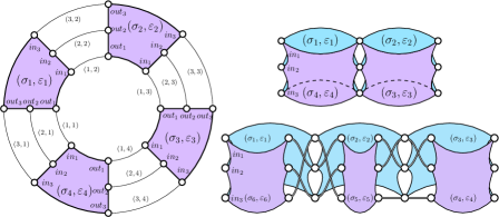
Figure 1: Representations of ^∗-test hypergraphs for $k=3$. Each hyperedge is pictured as a square with its $k$ outputs represented on an edge in clockwise order, and its $k$ inputs in the opposite face in anti-clockwise order. The links between vertices represent identifications. The symbols $(\sigma_{i},\epsilon_{j})$ indicate the labels of the hyperedges. Left: the graph $T_{\sigma_{1},\ldots,\sigma_{4}}^{\varepsilon_{1},\ldots,\varepsilon_{4}}$. Right: two graphs that are commented in Section 5.3.

The hypergraph $T_{\sigma_{1},\ldots,\sigma_{L}}^{\varepsilon_{1},\ldots,\varepsilon_{L}}$ consists in a strip with $\ell$ successive hyperedges, see the left panel of Figure 1. We then have in particular for a ^∗-test hypergraph of the form $T=T_{\sigma_{1},\ldots,\sigma_{L}}^{\varepsilon_{1},\ldots,\varepsilon_{L}}$

$$\Phi_{N}\big{[}M_{N,\sigma_{1}}^{\varepsilon_{1}}\cdots M_{N,\sigma_{L}}^{\varepsilon_{L}}\big{]}=\mathbb{E}\left[\frac{1}{N^{k}}\mathrm{Tr}\big{[}T_{\sigma_{1},\ldots,\sigma_{L}}^{\varepsilon_{1},\ldots,\varepsilon_{L}}(M_{N})\big{]}\right],$$ (5.3)

showing how we can encode the ^∗-moments of the flattenings of $M_{N}$ using hypergraphs.

We now define a modification of the trace of ^∗-test hypergraphs.

Definition 5.3.

The injective trace of a ^∗-test hypergraph $T$ in $M_{N}$, denoted $\mathrm{Tr}^{0}\big{[}T(M_{N})\big{]}$, is defined as $\mathrm{Tr}\big{[}T(M_{N})\big{]}$ in (5.2) but with the summation restricted to the set of injective maps $j:V\to[N]$.

This functional $\mathrm{Tr}^{0}$ is related to the trace of ^∗-test hypergraphs thanks to Lemma 5.5, which requires the following definition.

Definition 5.4.

Let $T=(V,E,\sigma,\varepsilon)$ be a ^∗-test hypergraph. We denote by $\mathcal{P}(V)$ the set of partitions of the vertex set $V$. Then for any $\pi\in\mathcal{P}(V)$, we define the ^∗-test hypergraph

$$T^{\pi}=(V^{\pi},E^{\pi},\sigma^{\pi},\varepsilon^{\pi}),$$

called the quotient of $T$ by $\pi$, by

• $V^{\pi}=\pi$, i.e. a vertex is a block of $\pi$,

• each hyperedge $e_{\ell}=(i_{s})_{s\in[2k]}\in E$ induces a hyperedge $e^{\pi}_{\ell}=(B_{s})_{s\in[2k]}$, where $B_{s}$ is the block of $\pi$ containing $i_{s}$ for all $s\in[2k]$, and the labels of $e^{\pi}_{\ell}$ are $\sigma^{\pi}(e^{\pi}_{\ell})=\sigma(e_{\ell})$ and $\varepsilon^{\pi}(e^{\pi}_{\ell})=\varepsilon(e_{\ell})$.

Note that $T^{\pi}$ can possibly have multiple hyperedges even if $T$ does not have any, as in the top right picture of Figure 1. It also can have degenerated hyperedges $(B_{s})_{s\in[2k]}$ where $B_{s}=B_{s^{\prime}}$ for some $s\neq s^{\prime}$ in $[2k]$ (see Figure 2).

Lemma 5.5.

For any ^∗-test hypergraph $T$, we have

$$\mathrm{Tr}\big{[}T(M_{N})\big{]}=\sum_{\pi\in\mathcal{P}(V)}\mathrm{Tr}^{0}\big{[}T^{\pi}(M_{N})\big{]}.$$

Since any ^∗-moment (5.1) can be written as a trace of ^∗-test hypergraph by (5.3), Lemma 5.5 implies that any ^∗-moment is a finite sum of normalized injective trace of the form (5.4). The interest of this formulation is that the computation of injective traces is quite straightforward, and transforms the computation into a combinatorial problem.

Proof.

Let $j:V\to[N]$ be a map. We denote by $\ker j$ the partition of $V$ such that $v\sim_{\ker j}v^{\prime}$ whenever $j(v)=j(v^{\prime})$. One can write

$$\mathrm{Tr}\big{[}T(M_{N})\big{]}=\sum_{\pi\in\mathcal{P}(V)}\left(\sum_{\begin{subarray}{c}j:V\to[N]\\ \mathrm{s.t.\leavevmode\nobreak\ }\ker j=\pi\end{subarray}}\ \prod_{\begin{subarray}{c}e\in E\end{subarray}}\ M_{N,\sigma(e)}^{\varepsilon(e)}\big{(}j(e)\big{)}\right)$$

The lemma follows since the term in parenthesis equals $\mathrm{Tr}^{0}\big{[}T^{\pi}(M_{N})\big{]}$. ∎

We also define

$$\tau_{N}^{0}[T^{\pi}] := \mathbb{E}\Big{[}\frac{1}{N^{k}}\mathrm{Tr}^{0}\big{[}T^{\pi}(M_{N})\big{]}\Big{]}.$$ (5.4)

5.2 Expression of injective traces under Hypothesis 1.2

In this section we set up the definitions needed for writing an exact expression of $\tau_{N}^{0}[T^{\pi}]$ defined in (5.4), for any ^∗-test hypergraph $T=(V,E,\sigma,\varepsilon)$ and any partition $\pi$ of its vertex set $V$. We assume $N\geq|V^{\pi}|$ since otherwise $\tau_{N}^{0}[T^{\pi}]=0$. In order to regroup terms in our computation, we need the following definition. We use as before the notation $j(e):=\big{(}j(v_{1}),\ldots,j(v_{2k})\big{)}$ for an hyperedge $e=(v_{1},\ldots,v_{2k})$ and a function $j:V^{\pi}\to[N]$.

Definition 5.6.

Let $T$ be a ^∗-test hypergraph and $\pi$ be a partition of its vertex set.

1. We say that two hyperedges $e$ and $e^{\prime}$ of $T^{\pi}$ are dependent whenever, for any $j:V^{\pi}\to[N]$ injective, $M_{N,\sigma(e)}^{\varepsilon(e)}\big{(}j(e)\big{)}$ and $M_{N,\sigma(e^{\prime})}^{\varepsilon(e^{\prime})}\big{(}j(e^{\prime})\big{)}$ are either the same random variable or are complex conjugate of each other. We denote by $\hat{E}^{\pi}$ the set of equivalent classes of hyperedges for the relation of dependence.

2. For each class of dependence $\hat{e}$ in $\hat{E}^{\pi}$, we denote by $m(\hat{e})$ and $n(\hat{e})$ the number of hyperedges $e$ of $T^{\pi}$ in $\hat{e}$ such that $\varepsilon(e)=1$ and $\varepsilon(e)=*$ respectively. Let $x$ be distributed as the entries of $M_{N}$. Then we call weight of $T^{\pi}$ the quantity

   $$\omega_{N}[T^{\pi}] := \prod_{\hat{e}\in\hat{E}^{\pi}}N^{k}\times\mathbb{E}\big{[}x^{m(\hat{e})}\overline{x}^{n(\hat{e})}\big{]},$$ (5.5)

Note that by independence of the entries of $M_{N}$, the notion of dependence does not depend on the injective map $j$.

Remark 5.7.

Let $e$ be an hyperedge, and assume that its vertices in $T^{\pi}$ are pair-wise distinct. Then under Hypothesis 1.2 two entries $M_{N,\sigma(e)}^{\varepsilon(e)}\big{(}j(e)\big{)}$ and $M_{N,\sigma(e^{\prime})}^{\varepsilon(e^{\prime})}\big{(}j(e^{\prime})\big{)}$ are independent if and only if their covariance is zero. From the computation of covariances of Section 4, the hyperedges corresponding to these entries belong to a same class if $\varepsilon=\varepsilon^{\prime}$ and $\sigma=\sigma^{\prime}$, or $\varepsilon\neq\varepsilon^{\prime}$ and $\sigma=\tau\sigma^{\prime}$. Nonetheless if the vertices of the hyperedge are not distinct this is no longer true.

Lemma 5.8.

For any ^∗-test hypergraph $T$ and any a partition $\pi$ of its vertices, we have

$$\tau_{N}^{0}[T^{\pi}] = N^{-k-k|\hat{E}^{\pi}|}\frac{N!}{(N-|V^{\pi}|)!}\omega_{N}[T^{\pi}],$$ (5.6)

where $\omega_{N}[T^{\pi}]$ defined in (5.5) is bounded, $\omega_{N}[T^{\pi}]=0$ if there is an equivalent class of dependence with a single element, and $\omega_{N}[T^{\pi}]\underset{N\rightarrow\infty}{\longrightarrow}0$ if there is an equivalent class of dependence of cardinal different from 2.

Proof.

Since $M_{N}$ has i.i.d. entries, the definition of the injective trace gives (with the convention $0!=1$)

$$\tau_{N}^{0}[T^{\pi}] = \frac{1}{N^{k}}\sum_{\begin{subarray}{c}j:V\to[N]\\ \mathrm{injective}\end{subarray}}\ \mathbb{E}\Big{[}\prod_{\begin{subarray}{c}e\in E\end{subarray}}\ M_{N,\sigma(e)}^{\varepsilon(e)}\big{(}j(e)\big{)}\Big{]},$$ (5.7)

$$= N^{-k}\frac{N!}{\times(N-|V^{\pi}|)!}\mathbb{E}\bigg{[}\prod_{\begin{subarray}{c}e\in E\end{subarray}}\ M_{N,\sigma(e)}^{\varepsilon(e)}\big{(}j(e)\big{)}\bigg{]}$$

for any injective map $j:V^{\pi}\to[N]$. The value of the expectation is independent of the choice of $j$. Two edges are dependent whenever they contribute to the same entry in Formula (5.7), so

$$\mathbb{E}\bigg{[}\prod_{\begin{subarray}{c}e\in E\end{subarray}}\ M_{N,\sigma(e)}^{\varepsilon(e)}\big{(}j(e)\big{)}\bigg{]}=\prod_{\hat{e}\in\hat{E}^{\pi}}\mathbb{E}\Big{[}M_{N}\big{(}j(e)\big{)}^{m(\hat{e})}\overline{M_{N}\big{(}j(e)\big{)}}^{n(\hat{e})}\Big{]}.$$

Moreover, since the entries of $M_{N}$ are i.i.d., the expectations in the right hand side term above does not depend on the entry $j(e)$. It can be replaced by the entry $(\mathbf{1})$ without changing the value of the expectations. This gives the expected formula. The rest of the lemma is consequence of Hypothesis 1.2. ∎

The set $\hat{E}^{\pi}$ forms a partition of the set of hyperedges that depends in an intricate way on $\pi$, $\sigma$ and $\varepsilon$. We will overpass the dependence on $\sigma$ and $\varepsilon$ by introducing another graph. It will allow, after a combinatorial analysis, to assume that $\hat{E}^{\pi}$ is a pair partition before we need to compute $\omega_{N}[T^{\pi}]$, relating our problem with the computation of the $\mathfrak{S}_{k}$-covariances studied earlier.

5.3 Important examples

We consider the two ^∗-test hypergraphs $T^{\pi}$ from the rightmost pictures of Figure 1. We propose to compute explicitly $\tau_{N}^{0}[T^{\pi}]$ and its limit for each of these graphs.

5.3.1 A case with no twisting

We denote by $T_{1}$ the ^∗-test hypergraph of the top rightmost picture of Figure 1, namely it is the quotient $T^{\pi}$ of $T=T_{\sigma_{1},\ldots,\sigma_{4}}^{\varepsilon_{1},\ldots,\varepsilon_{4}}$ with $k=3$ for the partition $\pi$ that identifies the $i$-th output of the second hyperedge with the $i$-th input of the third one for $i=1,2,3$. Since the second and third hyperedges of $T_{1}$ share the same vertices and the same holds for the first and fourth one, each of these pair may form either a single class of dependence (consisting in two hyperedges) or two classes (consisting in single hyperedges). This depends on the values of the $\sigma_{i}$’s and $\varepsilon_{i}$’s. If there is a class of dependence formed by a single element, then $\tau_{N}^{0}[T_{1}]=0$ (Lemma 5.8).

By Remark 5.7, the second and the third hyperdeges of $T_{1}$ belong to a same class if and only if one of the following dependence conditions is satisfied: $\varepsilon_{2}\neq\varepsilon_{3}$ and $\sigma_{2}=\sigma_{3}$, $\varepsilon_{2}=\varepsilon_{3}$ and $\sigma_{2}=\tau\sigma_{3}$ where we recall that $\tau$ is defined as in Theorem 2.15

$$\tau(i) :  \left\{\begin{array}[]{ccc}i\in[k]&\mapsto&i+k\in[2k]\setminus[k]\\ i\in[2k]\setminus[k]&\mapsto&i-k\in[k].\end{array}\right.$$

Note the formal difference with the formula 5.7, since we must take into account that the way the two hyperedge are identified by identifying the inputs of one with the outputs of the other one. Using the notation $[1]=0$ and $[*]=1$, we shall write this dependence condition in short $\tau^{[\varepsilon_{2}]}\sigma_{2}=\tau^{1+[\varepsilon_{3}]}\sigma_{3}$. The similar condition of dependence holds for the first and fourth hyperedges.

Assume that these dependence conditions are satisfied, so $T^{\pi}$ has $|\hat{E}^{\pi}|=2$ classes of dependences. Note that $T_{1}$ has $|V_{1}^{\pi}|=9$ vertices. Hence we get

$$N^{-k-k|\hat{E}^{\pi}|}\frac{N!}{(N-|V^{\pi}|)!}=N^{-9}\frac{N!}{(N-9)!}.$$

It remains to write the expression of $\omega_{N}[T_{1}]$. Let $x$ be distributed as the entries of $M_{N}$. Denoting $x^{*}:=\bar{x}$ the usual complex conjugation, the definition of $\omega_{N}$ and the above computation finally yields the expression

$$\tau^{0}_{N}[T_{1}] = N^{-9}\frac{N!}{(N-9)!}\times\delta_{\tau^{[\varepsilon_{2}]}\sigma_{2},\tau^{1+[\varepsilon_{3}]}\sigma_{3}}\delta_{\tau^{[\varepsilon_{1}]}\sigma_{1},\tau^{1+[\varepsilon_{4}]}\sigma_{4}}$$

$$\ \ \ \ \times N^{k}\mathbb{E}[x^{\varepsilon_{2}}\bar{x}^{\varepsilon_{3}}]\times N^{k}\mathbb{E}[x^{\varepsilon_{1}}\bar{x}^{\varepsilon_{4}}],$$

where $\delta$ stands for the usual Kronecker symbol. Since $N^{-k-k|\hat{E}^{\pi}|}\frac{N!}{(N-|V^{\pi}|)!}$ converges to one, Hypothesis 1.2 implies that $\tau^{0}_{N}[T_{1}]$ converges when $N$ tends to infinity. Denoting by $(c,c^{\prime})$ the parameter of $M_{N}$, we get the expression of the limit using the formula

$$\underset{N\rightarrow\infty}{\lim}N^{k}\mathbb{E}[x^{\varepsilon}\bar{x}^{\varepsilon^{\prime}}]=\left\{\begin{array}[]{ccc}c&\mathrm{if}&\varepsilon\neq\varepsilon^{\prime},\\ c^{\prime}&\mathrm{if}&\varepsilon=\varepsilon^{\prime}=1,\\ \bar{c}^{\prime}&\mathrm{if}&\varepsilon=\varepsilon^{\prime}=*.\end{array} \right.$$

Finally, note that the computation of covariances of Section 4 shows that

$$\tau^{0}_{N}[T_{1}]=\Phi_{N}(M_{N,\sigma_{2}}^{\varepsilon_{2}}M_{N,\sigma_{3}}^{\varepsilon_{3}})\times\Phi_{N}(M_{N,\sigma_{1}}^{\varepsilon_{1}}M_{N,\sigma_{4}}^{\varepsilon_{4}})+o(1).$$

5.3.2 A case with twistings

We now denote by $T_{2}$ the ^∗-test hypergraph of the right bottom picture of Figure 1, namely it is the quotient $T^{\pi}$ of $T=T_{\sigma_{1},\ldots,\sigma_{6}}^{\varepsilon_{1},\ldots,\varepsilon_{6}}$ for the partition $\pi$ that does the following identifications:

• for $\eta_{1}$ the transposition exchanging 1 and 2, the $i$-th output of the third hyperedge is identified with the $\eta_{1}(i)$-th input of the fourth one,

• for $\eta_{2}$ is the cycle $(1,3,2)$, the $i$-th output of the second hyperedge is identified with the $\eta_{2}(i)$-th input of the fifth one.

The same reasoning as before shows that there are up to three classes of dependence, the pairs of indices of possible dependent hyperedges being $\{3,4\},\{2,5\}$ and $\{1,6\}$. The description of the depedent classes involves now the twisting induced by the permutations $\eta_{1}$ and $\eta_{2}$. Using the notation $[1]=0$ and $[*]=1$, we observe from the figure that each pair of indices $\{3,4\},\{2,5\}$ and $\{1,6\}$ corresponds to hyperedges of $T_{2}$ in a same class of dependence whenever the following dependence conditions are satisfied:

$$\left\{\begin{array}[]{ccc}\tau^{[\varepsilon_{3}]}\sigma_{3}&=&(\mu_{1}\sqcup\mathrm{id})\tau^{1+[\varepsilon_{4}]}\sigma_{4},\\ \tau^{[\varepsilon_{2}]}\sigma_{2}&=&(\mu_{2}\sqcup\mu_{1}^{-1})\tau^{1+[\varepsilon_{5}]}\sigma_{5},\\ \tau^{[\varepsilon_{1}]}\sigma_{1}&=&(\mathrm{id}\sqcup\mu_{2}^{-1})\tau^{\varepsilon_{6}}\tau^{1+[\varepsilon_{6}]}\sigma_{6}.\end{array}\right.$$

Indeed, let us consider the first formula. Since the role of the $\varepsilon$-indices is clear from the previous example, let us assume $(\varepsilon_{3},\varepsilon_{4})=(\varepsilon_{2},\varepsilon_{5})=(\varepsilon_{1},\varepsilon_{6})=(1,*)$ for a simplification that does not affect the reasoning. Therefore the condition reads $\sigma_{3}=(\mu_{1}\sqcup\mathrm{id})\sigma_{4}$. It is the consequence of Remark 5.7, the fact that by construction the $i$-th output of the third hyperedge is the $i$-th input of the fourth one, and the identification of vertices in the first item of the enumeration at the beginning of this subsection, namely of the $i$-th input of the third hyperedge is the $\eta_{1}(i)$-th output of the fourth one.

The second formula now reads $\sigma_{2}=(\mu_{2}\sqcup\mu_{1}^{-1})\sigma_{5}$, which follows from the second item of the above enumeration, and the fact that the first item implies that the $i$-th output of the second hyperedge is identified by $\pi$ with the $\eta_{1}^{-1}(i)$-th input of the fifth one. Similarly, the last formula reads $\sigma_{1}=(\mathrm{id}\sqcup\mu_{2}^{-1})\sigma_{6}$ with same arguments, the factor $\mathrm{id}$ coming from construction and the factor $\mu_{2}^{-1}$ for the second itemized identification condition.

When the dependence conditions are satisfied they are $|\hat{E}^{\pi}|=3$ dependent classes of hyperedges, and $T_{2}$ has $|V^{\pi}|=12$ vertices. With the same computation of the weights as in the previous section, Lemma 5.8 yields

$$\tau^{0}_{N}[T_{2}]$$

$$= \delta_{\tau^{[\varepsilon_{3}]}\sigma_{3},\mu_{1}\tau^{1+[\varepsilon_{4}]}\sigma_{4}}\delta_{\tau^{[\varepsilon_{2}]}\sigma_{2},\mu_{2}\tau^{1+[\varepsilon_{5}]}\sigma_{5}\mu_{1}^{-1}}\delta_{\tau^{[\varepsilon_{1}]}\sigma_{1},\tau^{\varepsilon_{6}}\tau^{1+[\varepsilon_{6}]}\sigma_{6}\mu_{2}^{-1}}$$

$$\ \ \ \ \times N^{-12}\frac{N!}{(N-12)!}\times\times N^{k}\mathbb{E}[x^{\varepsilon_{3}}\bar{x}^{\varepsilon_{4}}]\times N^{k}\mathbb{E}[x^{\varepsilon_{2}}\bar{x}^{\varepsilon_{5}}]\times N^{k}\mathbb{E}[x^{\varepsilon_{1}}\bar{x}^{\varepsilon_{6}}].$$

Hence under Hypothesis 1.2 $\tau^{0}_{N}[T_{2}]$ has a limit when $N$ tends to infinity. The computation of covariances made in the dedicated section shows

$$\tau^{0}_{N}[T^{\pi}] = \Phi_{N}(M_{N,\sigma_{3}}^{\varepsilon_{3}}M_{N,\mu_{1}\sigma_{4}}^{\varepsilon_{4}})\Phi_{N}(M_{N,\sigma_{2}}^{\varepsilon_{2}}M_{N,\mu_{2}\sigma_{5}\mu_{1}^{-1}}^{\varepsilon_{5}})$$

$$\ \ \ \ \times\Phi_{N}(M_{N,\sigma_{1}}^{\varepsilon_{1}}M_{N,\sigma_{6}\mu_{2}^{-1}}^{\varepsilon_{6}})\times+o(1).$$

Lemma 2.16 implies that

$$\Phi_{N}(M_{N,\sigma}^{\varepsilon}M_{N,\mu\sigma^{\prime}{\mu^{\prime}}^{-1}}^{\varepsilon^{\prime}})=\left\{\begin{array}[]{ccc}\Phi_{N}(M_{N,\sigma}^{\varepsilon}U_{N,\mu}M_{N,\sigma^{\prime}}U_{N,\mu^{\prime}}^{*})&\mathrm{if}&\varepsilon^{\prime}=1,\\ \Phi_{N}(M_{N,\sigma}^{\varepsilon}U_{N,\mu^{\prime}}M_{N,\sigma^{\prime}}^{*}U_{N,\mu}^{*})&\mathrm{if}&\varepsilon^{\prime}=*.\end{array}\right.$$

This is a first indication of the interest of introduction the $\mathfrak{S}_{k}$-probability setting.

5.4 Convergence of injective traces

In Lemma 5.8 we have established an exact formula for $\tau_{N}^{0}[T^{\pi}]$ involving the normalization factor

$$\frac{N!\times N^{|\hat{E}^{\pi}|}}{N^{k}\times(N-|V^{\pi}|)!}=\big{(}1+o(1)\big{)}\times N^{-k-|\hat{E}^{\pi}|+|V^{\pi}|},$$

where we recall that $|\hat{E}^{\pi}|$ is the number of classes of dependent edges $T^{\pi}$ and $|V^{\pi}|$ is the number of vertices of $T^{\pi}$.

In this section, we assume that $T=T_{\sigma_{1},\ldots,\sigma_{L}}^{\varepsilon_{1},\ldots,\varepsilon_{L}}$ is a ^∗-test hypergraph as in Definition 5.2 encoding a ^∗-moments, and assume that the class of dependent hyperedges of $T^{\pi}$ have at least two elements (this is the situation of interest according to Lemma 5.8). We prove that $-k-|\hat{E}^{\pi}|+|V^{\pi}|\leq 0$ and learn important properties on the case of equality. This allows us to deduce the convergence of the $\mathfrak{S}_{k}$-distribution and prepare the proof of the convergence toward a $\mathfrak{S}_{k}$-circular system.

The arguments use the following types of ”simplified“ hypergraphs.

Definition 5.9.

1. A simple undirected hypergraph a pair $(V,E)$ where

   • $V$ is a non-empty set;

   • $E$ is a set of subsets of elements of $V^{\ell}$ for some $1\leq\ell\leq 2k$.

2. For any partition $\pi$ of $V$, we set $\bar{T}^{\pi}=(V^{\pi},\bar{E}^{\pi})$, and call skeleton of $T^{\pi}$, the undirected hypergraph $(V^{\pi},\bar{E}^{\pi})$ where $\bar{E}^{\pi}$ is the set of all subsets of indices $\{v_{1},\ldots,v_{2k}\}$ such that $(v_{1},\ldots,v_{2k})\in E$. The fibre of $\bar{e}\in\bar{E}^{\pi}$ is the set of all $(v_{1},\ldots,v_{2k})\in E^{\pi}$ such that $\bar{e}=\{v_{1},\ldots,v_{2k}\}$.

We denote $q(\pi)=-k-k|\bar{E}^{\pi}|+|V^{\pi}|$, so that we can write

$$-k-|\hat{E}^{\pi}|+|V^{\pi}|=q(\pi)+k\big{(}|\bar{E}^{\pi}|-|\hat{E}^{\pi}|\big{)}.$$ (5.9)

Note that the skeleton of $T^{\pi}$ does not depend on the labelings $\sigma$ and $\varepsilon$. If two hyperedges of $T^{\pi}$ belong to a same class of dependence, then they are fibres of a same hyperedge in the skeleton of $T^{\pi}$. Hence $|\bar{E}^{\pi}|\leq|\hat{E}^{\pi}|$ with equality if and only if the fibres of the hyperedges of $\bar{T}^{\pi}$ coincide with the classes of dependence of $T^{\pi}$.

We prove that $q(\pi)\leq 0$ for any quotient $T^{\pi}$. The idea is to consider the evolution of the combinatorial quantities under interest (5.9) for the sequence of skeletons generated by the first $\ell$-th hyperedges of $T^{\pi}$ while $\ell$ increases (see Figure 2). More precisely, for any $\ell=1,\ldots,L-1$, let $S_{\ell}=(V_{\ell},E_{\ell})$ be the ^∗-test hypergraph consisting in a open strip with $\ell$ successive hyperedges and defined as follow

• $V_{\ell}=\{(1,1),\dots,(1,L-\ell),\dots,(k,1),\ldots,(k,L-\ell)\},$

• $E_{\ell}=\{e_{1},,\ldots,e_{\ell}\}$ where

  $$e_{i}=\big{(}(1,i+1),\ldots,(k,i+1),(1,i),\ldots,(k,i)\big{)}$$

  (each edge is of multiplicity one),

• for all $i=1,\ldots,\ell$, we have $\sigma(e_{i})=\sigma_{i},$ and $\varepsilon(e_{i})=\varepsilon_{i}$.

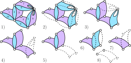
Figure 2: Picture 11: a ^∗-test hypergraph $T^{\pi}$, where the indicate the order of the hyperedges by indices from 1 to 10. Pictures 1 to 10 represent $S_{\ell}^{\pi}$ as $\ell$ increases from 1 to 10, with the last four steps regroups for conciseness. The dot lines and vertices represent the $i$-th hyperedge while the continuous lines represent $S^{\pi}_{i-1}$.

Let also denote $S_{L}=(V_{L},E_{L}):=T$, and let $S_{0}=(V_{0},\emptyset)$ be the hypergraph with $k$ isolated vertices $(1,1),\ldots,(k,1)$ and no hyperedge. For each $\ell=0,\ldots,L$, the partition $\pi$ induces a partition on $V_{\ell}$ (with a slight abuse of notation, we still denote it $\pi$) and so a quotient $S^{\pi}_{\ell}=(V^{\pi}_{\ell},E^{\pi}_{\ell})$ of $S_{\ell}$. For each $\ell=0,\ldots,L$, we set

$$q(\pi,\ell)=-k-k|\bar{E}_{\ell}^{\pi}|+|V_{\ell}^{\pi}|,$$ (5.10)

where $(V_{\ell}^{\pi},\bar{E}_{\ell}^{\pi})$ is the skeleton of $S^{\pi}_{\ell}$ (Definition 5.9).

Lemma 5.10.

For any ^∗-hypergraph of the form $T=T_{\sigma_{1},\ldots,\sigma_{L}}^{\varepsilon_{1},\ldots,\varepsilon_{L}}$ and for any partition $\pi$ of its vertices, the sequence $q(\pi,\ell)_{\ell=0,\ldots,L}$ is non-increasing and it satisfies $q(\pi,0)\leq 0$.

The lemma clearly implies that $q(\pi)=q(\pi,L)\leq 0$, as expected.

Proof.

The graph $S^{\pi}_{0}$ is the quotient of $k$ isolated vertices (the outputs of the first hyperedge $e_{1}$) so it consists of a number $a_{0}\in[k]$ of vertices. Hence we have $q(\pi,0)=-k+a_{0}\leq 0$ with equality if and only if $a_{0}=k$, i.e. the partition $\pi$ does not identify different outputs of $e_{1}$.

We consider the variation of the sequence, namely for $\ell=1,\ldots,L$

$$q(\pi,\ell)-q(\pi,\ell-1)=-k\big{(}|\bar{E}_{\ell}|-|\bar{E}_{\ell-1}|\big{)}+\big{(}|V_{\ell}^{\pi}|-|V_{\ell-1}^{\pi}|\big{)}.$$

For $\ell=1$, since the skeleton of $S_{1}^{\pi}$ has one hyperedge and $S_{0}^{\pi}$ has none, then $|\bar{E}_{1}|-|\bar{E}_{0}|=1$. Moreover, the vertices of $S_{1}$ that are not in $S_{0}$ (the $k$ inputs of $e_{1}$) can form up to $k$ new vertices in $S_{1}^{\pi}$. Setting $a_{1}:=|V_{1}^{\pi}|-|V_{0}^{\pi}|\in\{0,\ldots,k\}$, we then have $q(\pi,1)-q(\pi,0)=-k+a_{1}\leq 0$ with equality if and only if $a_{1}=k$, i.e. the partition $\pi$ does not identify different inputs of $e_{1}$, and does not identify an input of $e_{1}$ with a vertex consider early (at this step, these are the outputs of $e_{1}$).

We now come adding the other hyperedges $e_{2},\ldots,e_{L-1}$. For each hyperedge $e_{\ell}$, we face a choice:

1. Either it is of multiplicity one in the quotient $S^{\pi}_{\ell}$. In this case, the reasoning is the same as for $\ell=1$, namely we have $|\bar{E}_{\ell}|-|\bar{E}_{\ell-1}|=1$ and $a_{\ell}:=|V^{\pi}_{\ell}|-|V^{\pi}_{\ell-1}|\in\{0,\ldots,k\}$, so $q(\pi,\ell)-q(\pi,\ell-1)=-k+a_{\ell-1}\leq 0$. For next section, we refer this as a growth step.

2. Or $e_{\ell}$ is associated with other hyperedge to form a multiple hyperedge in $S^{\pi}_{\ell}$. This implies that the skeletons of $S^{\pi}_{\ell}$ and $S^{\pi}_{\ell-1}$ are the same, and so $q(\pi,\ell)=q(\pi,\ell-1)$. For next section, we refer this as a backtrack step.

By induction, this proves that $q(\pi,\ell)\leq q(\pi,\ell-1)$ for all $\ell=1,\ldots,L-1$.

Finally we add the last hyperedge. The vertex sets of $T$ and $S_{L-1}$ are the same, so $|V^{\pi}_{L}|-|V^{\pi}_{L-1}|=0$. Either $e_{L}$ is simple in $T^{\pi}$, in which case $|\bar{E}^{\pi}_{L}|-|\bar{E}^{\pi}_{L-1}|=1$ and so $q(\pi,L)=q(\pi,L-1)-k$, or it is multiple in $T^{\pi}$, in which case $q(\pi,L)=q(\pi,L-1)$. ∎

Now that we have proved the main result of this section, we can deduce easily the following convergence.

Corollary 5.11.

The collection of flattenings of a random tensor satisfying Hypothesis 1.2 converges in $\mathfrak{S}_{k}$-distribution.

Proof.

We shall prove the convergence of $\mathcal{E}_{N}\big{[}M_{N,\sigma_{1}}^{\varepsilon_{1}}U_{N,\eta_{1}}\cdots M_{N,\sigma_{L}}^{\varepsilon_{L}}U_{N,\eta_{L}}\big{]}$ for an arbitrary choice of $L\geq 1$, $\sigma_{\ell}\in\mathfrak{S}_{2k}$, $\varepsilon_{\ell}\in\{1,*\}$ and $\eta_{\ell}\in\mathfrak{S}_{k}$ for all $\ell\in[L]$. The definition of $\mathcal{E}_{N}$ and Lemma 2.16 yields

$$\mathcal{E}_{N}\big{[}M_{N,\sigma_{1}}^{\varepsilon_{1}}U_{N,\eta_{1}}\cdots M_{N,\sigma_{L}}^{\varepsilon_{L}}U_{N,\eta_{L}}\big{]}$$

$$= \sum_{\eta\in\mathfrak{S}_{k}}\Phi_{N}\big{[}M_{N,\sigma_{1}}^{\varepsilon_{1}}U_{N,\eta_{1}}\cdots M_{N,\sigma_{L}}^{\varepsilon_{L}}U_{N,\eta_{L}}U_{N,\eta^{-1}}\big{]}U_{N,\eta}$$

$$= \sum_{\eta\in\mathfrak{S}_{k}}\Phi_{N}\big{[}M_{N,\tilde{\sigma}_{1}}^{\varepsilon_{1}}\cdots M_{N,\tilde{\sigma}_{L}}^{\varepsilon_{L}}\big{]}U_{N,\eta},$$

where for $\ell=1,\ldots,L-1$, $\tilde{\sigma}_{\ell}=(\mathrm{id}\sqcup\eta_{\ell}^{-1})\sigma_{\ell}$ if $\varepsilon_{\ell}=1$ and $\tilde{\sigma}_{\ell}=(\eta_{\ell}^{-1}\sqcup\mathrm{id})\sigma_{\ell}$ if $\varepsilon_{\ell}=*$, and for $\ell=L$ we have $\tilde{\sigma}_{L}=(\mathrm{id}\sqcup\eta\eta_{L}^{-1})\sigma_{L}$ if $\varepsilon_{L}=1$ and $\tilde{\sigma}_{L}=(\eta\eta_{L}^{-1}\sqcup\mathrm{id})\sigma_{L}$ if $\varepsilon_{L}=*$.

We hence consider the ^∗-test graph $T=T_{\tilde{\sigma}_{1},\ldots,\tilde{\sigma}_{L}}^{\varepsilon_{1},\ldots,\varepsilon_{L}}$. We have

$$\Phi_{N}\big{[}M_{N,\tilde{\sigma}_{1}}^{\varepsilon_{1}}\cdots M_{N,\tilde{\sigma}_{L}}^{\varepsilon_{L}}\big{]} = \sum_{\pi\in\mathcal{P}(V)}\tau_{N}^{0}\big{[}T^{\pi}\big{]}.$$

Lemmas 5.8 and 5.10 prove that each term in the above sum converges. Hence we get the expected convergence and a formula for the limit

$$\Phi_{N}\big{[}M_{N,\tilde{\sigma}_{1}}^{\varepsilon_{1}}\cdots M_{N,\tilde{\sigma}_{L}}^{\varepsilon_{L}}\big{]} \underset{N\rightarrow\infty}{\longrightarrow} \sum_{\begin{subarray}{c}\pi\in\mathcal{P}(V)\mathrm{\ s.t.}\\ -k-|\hat{E}^{\pi}|+|V^{\pi}|=0\end{subarray}}\underset{N\rightarrow\infty}{\lim}\omega_{N}[T^{\pi}].$$ (5.11)

Let $\mathcal{A}$ be the free $\mathfrak{S}_{k}^{*}$-algebra generated by a family $(m_{\sigma})_{\sigma\in\mathfrak{S}_{k}}$ with relations $u_{\eta}m_{\sigma}u_{\eta^{\prime}}^{*}=m_{(\eta\sqcup\eta^{\prime})m_{\sigma}}$. We equip $\mathcal{A}$ with the linear map $\mathcal{E}$ defined by $\mathcal{E}\big{[}m_{\sigma_{1}}^{\varepsilon_{1}}u_{\eta_{1}}\cdots m_{\sigma_{L}}^{\varepsilon_{L}}u_{\eta_{L}}\big{]}=\underset{N\rightarrow\infty}{\lim}\mathcal{E}_{N}\big{[}M_{N,\sigma_{1}}^{\varepsilon_{1}}U_{N,\eta_{1}}\cdots M_{N,\sigma_{L}}^{\varepsilon_{L}}U_{N,\eta_{L}}\big{]}$. Therefore the collection of flattenings of $M_{N}$ converges to the family $\mathbf{m}=(m_{\sigma})_{\sigma\in\mathfrak{S}_{k}}$ in $\mathfrak{S}_{k}^{*}$-distribution. ∎

5.5 End of the proof

We prove that the limit of the flattenings computed in the previous section is $\mathfrak{S}_{k}$-circular, using the proof of Lemma 5.10 and manipulation explained in the second example in Section 5.3. We first state the following intermediate result, where we denote by $\mathrm{NC}_{2}(L)$ the sets of non-crossing pair partitions of $[L]$. We recall that for a sequence $\mathcal{L}_{n}$, $n\geq 1$, where $\mathcal{L}_{n}$ is a $n$-linear map, we define $\mathcal{L}_{\xi}$ for $\xi$ a non-crossing partition in Definition-Proposition 2.9.

Lemma 5.12.

Let $\mathbf{m}=(m_{\sigma})_{\sigma\in\mathfrak{S}_{k}}$ be the limit of the collection of flattenings given in Corollary 5.11. We set as usual $\phi(a)$ to be the coefficient of the identity in $\mathcal{E}(a)$, and we denote $\mathcal{A}lg^{*}(\mathbf{m})$ the ^∗-algebra generated by $\mathbf{m}$. There exists a collection $\mathcal{L}_{n}$, $n\geq 1$ of $n$-linear forms $\mathcal{A}lg^{*}(\mathbf{m})^{n}\to\mathbb{C}$, such that for all $L\geq 3$, all $\sigma_{1},\ldots,\sigma_{L}$ in $\mathfrak{S}_{2k}$ and all $\varepsilon_{1},\ldots,\varepsilon_{L}$ in $\{1,*\}$, we have

$$\phi\big{[}m_{\sigma_{1}}^{\varepsilon_{1}}\cdots m_{\sigma_{L}}^{\varepsilon_{L}}\big{]}$$

$$= \sum_{\xi\in\mathrm{NC}_{2}(L)}\mathcal{L}_{\xi\setminus B}\Big{[}m_{\sigma_{1}}^{\varepsilon_{1}},\ldots,m_{\sigma_{i-1}}^{\varepsilon_{i-1}}\mathcal{E}\big{[}m_{\sigma_{i}}^{\varepsilon_{i}}m_{\sigma_{i+1}}^{\varepsilon_{i+1}}\big{]},m_{\sigma_{i+2}}^{\varepsilon_{i-1}},\ldots,m_{\sigma_{L}}^{\varepsilon_{L}}\Big{]},$$

where $B=B(\xi)=\{i,i+1\}$ denotes the first internal block of $\xi$.

Proof.

Let $\pi$ be a partition of the ^∗-test hypergraph $T=T_{\sigma_{1},\ldots,\sigma_{L}}^{\varepsilon_{1},\ldots,\varepsilon_{L}}$, and with the notations of Lemma 5.8, assume that $-k-|\hat{E}^{\pi}|+|V^{\pi}|=0$. Section 5.4 proves that necessarily the class of dependence of the graph $T^{\pi}$ are of cardinal 2. Given such a $\pi$, we denote by $\xi(\pi)\in\mathcal{P}(L)$ the pair partition whose blocks are the pairs $\{\ell,\ell^{\prime}\}$ of indices such that the hyperedges $e_{\ell}$ and $e_{\ell^{\prime}}$ belong to a same class. Denoting by $\mathcal{P}_{2}(L)$ the set of pair partitions of $[L]$, we set for any $\xi\in\mathcal{P}_{2}(L)$

$$\mathcal{M}_{\xi}\Big{[}m_{\sigma_{1}}^{\varepsilon_{1}}\cdots m_{\sigma_{L}}^{\varepsilon_{L}}\Big{]} := \sum_{\begin{subarray}{c}\pi\in\mathcal{P}(V)\mathrm{\ s.t.}\\ -k-|\hat{E}^{\pi}|+|V^{\pi}|=0\\ \mathrm{and}\ \xi(\pi)=\xi\end{subarray}}\underset{N\rightarrow\infty}{\lim}\omega_{N}[T^{\pi}].$$

By our previous computation of the limit, namely (5.11) with $\eta_{1}=,\ldots,=\eta_{L}=\mathrm{id}$, we obtained that $\phi\big{[}m_{\sigma_{1}}^{\varepsilon_{1}}\cdots m_{\sigma_{L}}^{\varepsilon_{L}}\big{]}=\sum_{\xi\in\mathcal{P}_{2}(L)}\mathcal{M}_{\xi}\big{[}m_{\sigma_{1}}^{\varepsilon_{1}}\cdots m_{\sigma_{L}}^{\varepsilon_{L}}\big{]}$. Note in particular that the limit is zero if $L$ is odd.

Firstly, we shall prove that $\mathcal{M}_{\xi}\big{[}m_{\sigma_{1}}^{\varepsilon_{1}}\cdots m_{\sigma_{L}}^{\varepsilon_{L}}\big{]}=0$ if $\xi$ is not a non-crossing partition. Assume $L\geq 4$ is even. Recall that a pair partition $\xi$ is non-crossing if and only if there exists a internal block $B$ and the partition $\xi\setminus B$ is non-crossing. Let us prove that $\xi(\pi)$ satisfies this property when $-k-|\hat{E}^{\pi}|+|V^{\pi}|=0$. Recall the proof of Lemma 5.10: if $-k-|\hat{E}^{\pi}|+|V^{\pi}|=0$, this means that the difference $q(\pi,\ell)-q(\pi,\ell-1)$ of the combinatorial quantities defined in (5.10) is zero for all $\ell=1,\ldots,L$. Let $i+1$ be the first index such that the $(i+1)$-th step is a backtrack one. Then by construction $B=(i,i+1)$ is a block of $\xi(\pi)$. Now removing the block $B$ from $\xi(\pi)$ yields the partition $\tilde{\xi}(\pi)=\xi(\pi)\setminus B$. But the partition $\tilde{\xi}(\pi)$ is involved for the computation of $\phi\big{[}m_{\sigma_{1}}^{\varepsilon_{1}}\cdots m_{\sigma_{i-1}}^{\varepsilon_{i-1}}\times m_{\sigma_{i+2}}^{\varepsilon_{i+2}}\cdots m_{\sigma_{L}}^{\varepsilon_{L}}\big{]}$ in the same way $\xi$ is involved in the computation of the moment under consideration. Hence by induction on $L$, we get that $\xi(\pi)$ is a non crossing partition.

It now remains to prove that for each $\xi\in\mathcal{P}_{2}(L)$ we have $\mathcal{M}_{\xi}\big{[}m_{\sigma_{1}}^{\varepsilon_{1}}\cdots m_{\sigma_{L}}^{\varepsilon_{L}}\big{]}=M_{\xi\setminus B}\Big{[}m_{\sigma_{1}}^{\varepsilon_{1}},\ldots,m_{\sigma_{i-1}}^{\varepsilon_{i-1}}\mathcal{E}\big{[}m_{\sigma_{i}}^{\varepsilon_{i}}m_{\sigma_{i+1}}^{\varepsilon_{i+1}}\big{]},m_{\sigma_{i+2}}^{\varepsilon_{i-1}},\ldots,m_{\sigma_{L}}^{\varepsilon_{L}}\Big{]}$. Again, we come back to the proof of Lemma 5.10. During the first backtrack step, the the $j$-th input of the hyperedge $e_{i+1}$ is identified by $\pi$ with the $\eta_{\pi}(j)$-th output of $e_{i}$, for some twisting permutation $\eta_{\pi}$ of $[k]$. Therefore this situation is similar to the second example in Section 5.3.

The weight associated to the block $(i,i+1)\in\xi(\pi)$ with specified twisting given by a permutation $\eta_{\pi}$ is

$$\lim_{N\rightarrow\infty}N^{k}\mathbb{E}[M_{N,\sigma_{i}}^{\varepsilon_{i}}(\mathbf{a},\mathbf{b})(M_{N,\sigma_{i+1}}^{\varepsilon_{i+1}}U_{N,\eta_{\pi}})((\mathbf{b},\mathbf{a}))],$$

where $(\mathbf{a},\mathbf{b})$ denote the indices of the matrix elements and are all distinct (recall that both $\mathbf{a},\mathbf{b}$ are multiplets of $k$ elements and the resulting $2k$ elements are distinct). It is the weight appearing in the factorization of $\omega_{N}[T^{\pi}]$ over classes of dependence (see Formula 5.5 and proof of lemma 5.8). Moreover, since the inputs of the hyperedge associated to $M_{N,\sigma_{i+2}}^{\varepsilon_{i+2}}$ are identified with the outputs of the one associated to $M_{N,\sigma_{i+1}}^{\varepsilon_{i+1}}$, the conjugate of the twisting permutation appears on input vertices of the hyperedge associated to $M_{N,\sigma_{i+2}}^{\varepsilon_{i+2}}$ in $\omega_{N}[T^{\pi}]$ to correct for the introduction of the permutation $U_{N,\eta_{\pi}}$ above. This induces the identification of the outputs of $M_{N,\sigma_{i-1}}^{\varepsilon_{i-1}}$ with the inputs of $M_{N,\sigma_{i+2}}^{\varepsilon_{i+2}}$ through the permutation $U_{N,\eta_{\pi}}^{*}$. See Figure 3 for illustration. This identification is achieved by introducing $U_{N,\eta_{\pi}}^{*}$ in front of the factorized weight

$$\lim_{N\rightarrow\infty}N^{k}\mathbb{E}[M_{N,\sigma_{i}}^{\varepsilon_{i}}(\mathbf{a},\mathbf{b})(M_{N,\sigma_{i+1}}^{\varepsilon_{i+1}}U_{N,\eta_{\pi}})((\mathbf{b},\mathbf{a}))].$$

Note the fact that partitions $\pi$ mapping to the same partition $\xi(\pi)=\xi$ differs only by their induced twisting permutations. Therefore the weight associated to $B=(i,i+1)\in\xi$ in the expression of $\mathcal{M}_{\xi}$ is the sum over twisting permutations $\eta$ of the weights associated to the same block in $\xi(\pi)$ whose twisting permutation induced by $\pi$ is $\eta$. Hence, more formally the weight of the block $B$ is

$$\sum_{\eta\in\mathfrak{S}_{k}}\lim_{N\rightarrow\infty}N^{k}\mathbb{E}[M_{N,\sigma_{i}}^{\varepsilon_{i}}(\mathbf{a},\mathbf{b})(M_{N,\sigma_{i+1}}^{\varepsilon_{i+1}}U_{N,\eta})((\mathbf{b},\mathbf{a}))]U_{N,\eta}^{*}.$$

It is simple to recognize from the earlier workings the $\mathfrak{S}_{k}$-covariance $\mathcal{E}[m_{\sigma_{i}}^{\varepsilon_{i}}m_{\sigma_{i+1}}^{\varepsilon_{i+1}}]$ in the above formula. Therefore, we have shown that

$$\mathcal{M}_{\xi}[m_{\sigma_{1}}^{\varepsilon_{1}},\ldots,m_{\sigma_{i-1}}^{\varepsilon_{i-1}},m_{\sigma_{i}}^{\varepsilon_{i}},m_{\sigma_{i+1}}^{\varepsilon_{i+1}},m_{\sigma_{i+2}}^{\varepsilon_{i+2}},\ldots,m_{\sigma_{L}}^{\varepsilon_{L}}]=\\ \mathcal{M}_{\xi\setminus B}[m_{\sigma_{1}}^{\varepsilon_{1}},\ldots,m_{\sigma_{i-1}}^{\varepsilon_{i-1}}\mathcal{E}[m_{\sigma_{i}}^{\varepsilon_{i}}m_{\sigma_{i+1}}^{\varepsilon_{i+1}}],m_{\sigma_{i+2}}^{\varepsilon_{i+2}},\ldots,m_{\sigma_{L}}^{\varepsilon_{L}}].$$ (5.12)

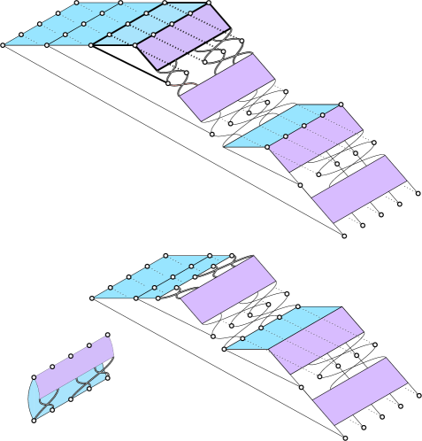
Figure 3: Top: for $k=5$, we represent a quotient $T^{\pi}$ of a graph $T=T_{\sigma_{1},\ldots,\sigma_{8}}^{\varepsilon_{1},\ldots,\varepsilon_{8}}$ for a partition $\pi$ that possibly contribute in the limit $\tau^{0}[T^{\pi}]$. We have $\xi(\pi)=\big{\{}\{1,8\},\{2,5\},\{3,4\},\{6,7\}\big{\}}$, and, in cycle decompositon $\eta_{1}:\{(1,2),(3,5,4)\}$, $\eta_{2}=\{(1,2,4),(3,5)\}$ and $\eta_{3}=\{(1),(2,5),(3),(4)\}$. The black lines represent identifications between vertices. We emphasize the hyperedges forming the first interval block $\{3,4\}$ of $\xi(\pi)$ and their identifications with heavier lines. Bottom left: we consider the two hyperedges $\{3,4\}$ solely and identify the $j$-th input of 4 with the $\eta_{1}^{-1}(j)$-th output of 3. Bottom right: We represent the quotient ${T^{\prime}}^{\pi^{\prime}}$ of the graph $T^{\prime}=T_{\sigma^{\prime}_{1},\ldots,\sigma^{\prime}_{6}}^{\varepsilon^{\prime}_{1},\ldots,\varepsilon^{\prime}_{8}}$ where $(\sigma^{\prime}_{1},\varepsilon^{\prime}_{1})=(\sigma_{1},\varepsilon_{1})$, $(\sigma^{\prime}_{2},\varepsilon^{\prime}_{2})=\big{(}(\mathrm{id}\sqcup\eta_{1})\sigma_{2},1\big{)}$ if $\varepsilon_{2}=1$ and $(\sigma^{\prime}_{2},\varepsilon^{\prime}_{2})=\big{(}(\eta_{1}\sqcup\mathrm{id})\sigma_{2},*\big{)}$ if $\varepsilon_{2}=*$, and $(\sigma^{\prime}_{i},\varepsilon_{i}^{\prime})=(\sigma_{i+2},\varepsilon_{i+2}^{\prime})$, for all $i\geq 3$.

∎

We can now finish the proof of our main theorem. As in the previous section, we have

$$\mathcal{E}\big{[}m_{\sigma_{1}}^{\varepsilon_{1}}u_{\eta_{1}}\cdots m_{\sigma_{L}}^{\varepsilon_{L}}u_{\eta_{L}}\big{]} = \sum_{\eta\in\mathfrak{S}_{k}}\Phi\big{[}m_{\tilde{\sigma}_{1}}^{\varepsilon_{1}}\cdots m_{\tilde{\sigma}_{L}}^{\varepsilon_{L}}\big{]}u_{\eta},$$

where for $\ell=1,\ldots,L-1$, $\tilde{\sigma}_{\ell}=(\mathrm{id}\sqcup\eta_{\ell}^{-1})\sigma_{\ell}$ if $\varepsilon_{\ell}=1$ and $\tilde{\sigma}_{\ell}=(\eta_{\ell}^{-1}\sqcup\mathrm{id})\sigma_{\ell}$ if $\varepsilon_{\ell}=*$, and for $\ell=L$ we have $\tilde{\sigma}_{L}=(\mathrm{id}\sqcup\eta\eta_{L}^{-1})\sigma_{L}$ if $\varepsilon_{L}=1$ and $\tilde{\sigma}_{L}=(\eta\eta_{L}^{-1}\sqcup\mathrm{id})\sigma_{L}$ if $\varepsilon_{L}=*$. Therefore we get from Lemma 5.12

$$\mathcal{E}\big{[}m_{\sigma_{1}}^{\varepsilon_{1}}u_{\eta_{1}}\cdots m_{\sigma_{L}}^{\varepsilon_{L}}u_{\eta_{L}}\big{]}$$

$$= \sum_{\xi\in\mathrm{NC}_{2}(L)}\sum_{\eta\in\mathfrak{S}_{k}}\mathcal{L}_{\xi\setminus B}\Big{[}m_{\tilde{\sigma}_{1}}^{\varepsilon_{1}},\ldots,m_{\tilde{\sigma}_{i-1}}^{\varepsilon_{i-1}}\mathcal{E}\big{[}m_{\tilde{\sigma}_{i}}^{\varepsilon_{i}}m_{\tilde{\sigma}_{i+1}}^{\varepsilon_{i+1}}\big{]},m_{\tilde{\sigma}_{i+2}}^{\varepsilon_{i-1}},\ldots,m_{\tilde{\sigma}_{L}}^{\varepsilon_{L}}\Big{]}u_{\eta}$$

Hence setting for each $n\geq 1$

$$\tilde{\mathcal{K}}_{n}(m_{\sigma_{1}}^{\varepsilon_{1}}u_{\eta_{1}},\ldots,m_{\sigma_{L}}^{\varepsilon_{L}}u_{\eta_{L}})=\left\{\begin{array}[]{ccc}\sum_{\eta\in\mathfrak{S}_{k}}\mathcal{L}(m_{\sigma_{1}}^{\varepsilon_{1}}u_{\eta_{1}}m_{\sigma_{2}}^{\varepsilon_{2}}u_{\eta_{2}}u_{\eta}^{*})u_{\eta}&\mathrm{if}n=2\\ 0&\mathrm{otherwise}\end{array}\right.$$

we have proved the sequence $\tilde{K}_{n},n\geq 1$ satisfies the moment-cumulant relation over $\mathfrak{S}_{k}$

$$\mathcal{E}\big{[}m_{\sigma_{1}}^{\varepsilon_{1}}u_{\eta_{1}}\cdots m_{\sigma_{L}}^{\varepsilon_{L}}u_{\eta_{L}}\big{]}$$

$$= \sum_{\xi\in\mathrm{NC}_{2}(L)}\tilde{\mathcal{K}}_{\xi\setminus B}\Big{[}m_{\sigma_{1}}^{\varepsilon_{1}}u_{\sigma_{1}},\ldots,m_{\sigma_{i-1}}^{\varepsilon_{i-1}}u_{\sigma_{-1}}\mathcal{E}\big{[}m_{\sigma_{i}}^{\varepsilon_{i}}u_{\sigma_{i}}m_{\sigma_{i+1}}^{\varepsilon_{i+1}}u_{\sigma_{i+1}}\big{]},$$

$$\ \ \ \ \ m_{\sigma_{i+2}}^{\varepsilon_{i-1}}u_{\sigma_{i+2}},\ldots,m_{\sigma_{L}}^{\varepsilon_{L}}u_{\sigma_{L}}\Big{]}.$$

By Definition-Proposition 2.11, necessarily $\tilde{K}_{n}=K_{n}$ for all $n\geq 1$ and by Definition 2.12, the family $(m_{\sigma})_{\sigma\in\mathfrak{S}_{k}}$ is $\mathfrak{S}_{k}$-circular.

References

- [AGV21] Benson Au and Jorge Garza-Vargas. Spectral asymptotics for contracted tensor ensembles. arXiv preprint arXiv:2110.01652, 2021.
- [BHS15] David John Baker, Hans Halvorson, and Noel Swanson. The conventionality of parastatistics. The British Journal for the Philosophy of Science, 66(4):929–976, 2015.
- [CDM16] Guillaume Cébron, Antoine Dahlqvist, and Camille Male. Traffic distributions and independence ii: universal constructions for traffic spaces. arXiv preprint arXiv:1601.00168, 2016.
- [DLN20] Stephane Dartois, Luca Lionni, and Ion Nechita. The joint distribution of the marginals of multipartite random quantum states. Random Matrices: Theory and Applications, 9(03):2050010, 2020.
- [DNT22] Stephane Dartois, Ion Nechita, and Adrian Tanasa. Entanglement criteria for the bosonic and fermionic induced ensembles. Quantum Information Processing, 21(11):1–46, 2022.
- [FH13] William Fulton and Joe Harris. Representation theory: a first course, volume 129. Springer Science & Business Media, 2013.
- [GSMZW09] Xin Geng, Kate Smith-Miles, Zhi-Hua Zhou, and Liang Wang. Face image modeling by multilinear subspace analysis with missing values. In Proceedings of the 17th ACM international conference on Multimedia, pages 629–632, 2009.
- [Har13] Aram W Harrow. The church of the symmetric subspace. arXiv preprint arXiv:1308.6595, 8 2013.
- [HGK10] Michiel Hazewinkel, Nadezhda Mikhailovna Gubareni, and Vladimir V Kirichenko. Algebras, rings and modules: Lie algebras and Hopf algebras, volume 3. American Mathematical Soc., 2010.
- [HHH02] Michal Horodecki, Pawel Horodecki, and Ryszard Horodecki. Separability of mixed quantum states: linear contractions approach. arXiv preprint quant-ph/0206008, 2002.
- [Jam84] James. The Representation Theory of the Symmetric Group. Encyclopedia of Mathematics and its Applications. Cambridge University Press, 1984.
- [Mal11] Camille Male. Traffic distributions and independence: permutation invariant random matrices and the three notions of independence. arXiv preprint arXiv:1111.4662, 2011.
- [MP16] James A Mingo and Mihai Popa. Freeness and the transposes of unitarily invariant random matrices. Journal of Functional Analysis, 271(4):883–921, 2016.
- [MS17] James A Mingo and Roland Speicher. Free probability and random matrices, volume 35. Springer, 2017.
- [Ott13] Giorgio Ottaviani. Introduction to the hyperdeterminant and to the rank of multidimensional matrices. In Commutative algebra, pages 609–638. Springer, 2013.
- [PM20] Mihai Popa and James A Mingo. The partial transpose and asymptotic free independence for wishart random matrices: Part ii. arXiv preprint arXiv:2005.04348, 2020.
- [PZ21] Soumik Pal and Yizhe Zhu. Community detection in the sparse hypergraph stochastic block model. Random Structures & Algorithms, 59(3):407–463, 2021.
- [RM14] Emile Richard and Andrea Montanari. A statistical model for tensor pca. Advances in neural information processing systems, 27, 2014.
- [Spe98] Roland Speicher. Combinatorial theory of the free product with amalgamation and operator-valued free probability theory, volume 627. American Mathematical Soc., 1998.
- [SS87] W.R. Scott and W.R. Scott. Group Theory. Dover Books on Mathematics. Dover Publications, 1987.
- [Wat18] John Watrous. The Theory of Quantum Information. Cambridge University Press, 2018.
- [WG03] Tzu-Chieh Wei and Paul M Goldbart. Geometric measure of entanglement and applications to bipartite and multipartite quantum states. Physical Review A, 68(4):042307, 2003.