Neural Operators for Delay-Compensating Control
of Hyperbolic PIDEs

Abstract

The recently introduced DeepONet operator-learning framework for PDE control is extended from the results for basic hyperbolic and parabolic PDEs to an advanced hyperbolic class that involves delays on both the state and the system output or input. The PDE backstepping design produces gain functions that are outputs of a nonlinear operator, mapping functions on a spatial domain into functions on a spatial domain, and where this gain-generating operator’s inputs are the PDE’s coefficients. The operator is approximated with a DeepONet neural network to a degree of accuracy that is provably arbitrarily tight. Once we produce this approximation-theoretic result in infinite dimension, with it we establish stability in closed loop under feedback that employs approximate gains.

In addition to supplying such results under full-state feedback, we also develop DeepONet-approximated observers and output-feedback laws and prove their own stabilizing properties under neural operator approximations. With numerical simulations we illustrate the theoretical results and quantify the numerical effort savings, which are of two orders of magnitude, thanks to replacing the numerical PDE solving with the DeepONet.

1 Introduction

In [7, 25], a method was introduced to pre-train the backstepping methodology, offline and once and for all, for certain entire classes of PDEs so that the implementation of the controller to any specific PDE within the class is nothing more than a function evaluation of a neural network that produces the controller gains based on the specific plant coefficients of the PDE being controlled.

In this paper, we extend this method to a broader and more advanced class of hyperbolic partial integro-differential systems, which involve delays on the state and the output or input.

1.1 The broader context of learning-based and data-driven control

Recently, learning-based control approaches have attracted great attention due to their leveraging of capabilities of deep neural networks. Some of these approaches learn control strategies from data without explicit knowledge of system dynamics, and some are able to deal with uncertainties and disturbances. Stability and robustness can be proven with some of these control methods [24], which builds trust for their use in practice. Progress has taken place with learning-based model predictive control (MPC) for uncertain models [38, 33], Lyapunov functional based control design [2, 50], reinforcement learning (RL) based linear quadratic regulator [32, 20], and other methods. RL has also been applied to PID tuning [16, 31], with a notable use in [27], where a deep RL-based PID tuning method is proposed and experimented on the physical two-tank system without prior pre-training. For the risks that might arise during the RL based control process, recently, safe reinforcement learning has emerged as a new research focus, see e.g., [17, 37, 48].

Learning-based control in unmanned systems is pursued in [9, 49, 28, 44]. For example in control of the unmanned aerial vehicles (UAVs), a dual-stream Actor-Critic network structure is applied to extract environmental features, enabling UAVs to safely navigate in environments with multiple obstacles[47]. Data-driven control methods extract the hidden patterns from a large amount of data, which improves control performance in uncertain environment. In [34], a deep network learning-based trajectory tracking controller, called Neural-Fly, is proposed for drones’ agile flight in rapidly changing strong winds. Transfer learning also used to leverage control strategies and models that have already been learned to accelerate the learning and adaptation process for new tasks, e.g., [41, 11, 28].

1.2 Learning-enhanced PDE control

Many engineering problems are spatio-temporal processes, often modeled by partial differential equations (PDEs) instead of ordinary differential equations (ODEs), such as plug flow reactor [45], traffic flow [36, 46], hydraulics and river dynamics [6], pipeline networks [1, 3], melt spinning processes [19], flexible robots [22], flexible satellite [21], tokamaks [30] and so on.

PDE backstepping has been particularly effective in the stabilization of PDEs. Since this paper is focused on a hyperbolic PIDE class, we mention only a few designs for hyperbolic systems here. A design for a single hyperbolic PIDE was introduced in [26]. A pair of coupled hyperbolic PDEs was stabilized next, with a single boundary input in [12]. An extension to $n+1$ hyperbolic PDEs with a single input was introduced in [15], an extension to cascades with ODEs in [14], an extension to “sandwiched” ODE-PDE-ODE systems in [42, 43], and redesigns robust to delays in [4, 5].

The dynamics of the PDE systems are defined in infinite-dimensional function spaces, so the gains in the PDE control systems (feedback controllers, observers, identifiers) are not vectors or matrices but functions of spatial arguments. When the coefficients of the system are spatially-varying, the equations governing the control gain kernels usually cannot be solved explicitly, as they are complex PDEs and need to be solved numerically, e.g. [15, 23, 39, 40]. When any coefficient changes, the control gain PDEs need to be re-solved, which is burdensome even if performed offline and once, let alone if it needs to be performed repeatedly in real time, in the context of adaptive control or gain scheduling.

It is of interest to find a neural network (NN) which learns control gain operators from a large set of previously offline-solved control design problems for a sample set of PDEs in a certain class. The DeepONet framework [7, 25] is an efficient method for PDE control, because it not only speeds up computation, e.g., on the order of magnitude of $10^{3}$ time [25], as compared to solving for the control gains numerically, but also provides a methodology for stability analysis. The DeepONet [29] consists of two sub-networks, i.e., branch net and trunk net. The branch net encodes the discrete input function space and the trunk encodes the domain of the output functions. The combination of branch and trunk nets improves the generalization and efficiency of operators learning of the DeepONet, so that it realize the regression of infinite-dimensional functions from a relatively small number of datasets [13], which brings new insights for the learning based control. Furthermore, the universal approximation theorem [29, 13, 10], which states that a nonlinear continuous operator can be approximated by an appropriate DeepONet with any given approximation error, provides the basis for the rigorous stability analysis of the closed-loop system under the neural operator controller.

This offline learning PDE control design framework was pioneered in [7]. Among the PDE control design approaches, PDE backstepping was used, due to its non-reliance on model reduction and its avoidance of numerically daunting operator Riccati equations. Among the neural operator methods, the DeepONet [29, 13] approach was employed, due to its availability of universal approximation theorem in infinite dimension. Closed-loop stability is guaranteed under the off-line trained NN-approximation of the feedback gains. Paper [25] extends this framework from first-order hyperbolic PDEs to a more complex class of parabolic PDEs whose kernels are governed by second-order PDEs, raising the difficulty for solving such PDEs and for proving the sufficient smoothness of their solutions, so that the neural operator (NO) approximations have guarantee of sufficient accuracy. Furthermore, an operator learning framework for accelerating nonlinear adaptive control is proposed in [8], where three operators are trained, namely parameter identifier operator, controller gain operator, and control operator.

1.3 Results, contributions, and organization of the paper

In this paper, we employ the DeepONet framework to learn the control kernel functions and the observer gains for the output feedback of a delayed first-order hyperbolic partial integro-differential equation (PIDE) system. Due to the system incorporating state and measurement or actuation delays, two transport PDEs are introduced to represent the delayed states, thus forming a hyperbolic PDEs cascade system. Applying the backstepping transformation, we derive a set of coupled PIDEs that three backstepping kernels should satisfy, the solution of which can only be obtained numerically. Hence, three DeepONets are trained to approximate the three kernel functions from the numerical solutions. Once the neural operators are trained from data, the kernel equations donot need to be solved numerically again for new functional coefficients and new delays.

We use the universal approximation theorem to prove the existence of DeepONet approximations, with an arbitrary accuracy, of the exact continuous operators mapping the delay and the system coefficient functions into kernel functions. Based on the approximation result, we provide a state-feedback stability guarantee under neural operator kernels by using a Lyapunov functional.

We incorporate a “dead-time” into our PIDE model. Dead-time can represent either actuation or sensing delay—when the full state is unmeasured, the delay can be shifted between the input and the output. Without loss of generality, we locate the delay at the output/measurement. In such an architecture, control requires the design of an observer for the unmeasured state. Due to the delayed measurement, the backstepping transformation for the observer design and analysis contains four kernels, which determine two observer gains. We use two DeepONets to learn the observer gains directly, instead of the four kernel functions.

The observer with gains produced by neural operators is proved to converge to the actual states. Moreover, we prove the stability of the output feedback system under the neural gains through constructing a new Lyapunov functional. Within the proof, we combine the system under prescribed stabilizing controller with the feedback of the estimated states and the observer error system to establish the exponentially stability, thus verifying the separation principle. We demonstrate the theoretical results with numerical tests and the corresponding code is available on github.

The paper’s main contribution is the following:

• Unlike the two inaugural papers [7, 25], this paper considers a PDE control problem subject to delays. The delayed system brings new challenges of dealing with multi-kernel coupled PDEs, for which we train three NNs to approximate three control kernels and two NNs to approximate two observer gains.

The paper’s additional contributions are:

• We combine the observer error system with the closed-loop system under the estimated state feedback to establish the exponentially stability, which verify the separation principle under the DeepONets learned output feedback controller.

• We train two DeepONets to approximate the two observer gains instead of four kernel functions, which cuts the offline training computation cost in half.

The paper is organized as follows. Section 2 briefly introduces the backstepping design of state feedback. In Section 3, we provides the existence of DeepONets approximations of the kernel functions to any accuracy. Section 4 proves that the closed-loop stability is guaranteed by the state feedback with the DeepONets control gains. The convergence of a backstepping observer that employs a DeepONet approximation of the observer gains is proved in Section 5 In Section 6 we combine the DeepONets-based state feedback and the observer to establish the closed-loop stability of the DeepONets output feedback. We illustrate the theoretical results with numerical examples in Section 7.

Notation: Throughout the paper, we adopt the following notations to for functions’ domain.

$${\mathcal{T}}_{1} =\left\{(s,q):0\leq s\leq q\leq 1\right\},$$ (1)

$${\mathcal{T}}_{2} =\left\{(s,r):~{}0\leq s,~{}r\leq 1\right\},$$ (2)

$${\mathcal{T}}_{3} =\left\{(s,q):~{}0\leq q\leq s\leq 1,\right\},$$ (3)

$$\underline{C} =\left\{c\in C^{1}[0,1]:~{}c(1)=0\right\}.$$ (4)

For $f\in L^{2}[0,1]$, denote the $L^{2}$ norm of $f$ by

$$\|f\|_{L^{2}}^{2}:=\int_{0}^{1}f^{2}(s,t)ds.$$ (5)

2 Output and State Delay Compensation by State-Feedback Backstepping

We consider the following PIDE system with state and sensor delay

$$x_{t}(s,t)= -x_{s}(s,t)+c(s)x(1,t-\tau)$$

$$~{}+\int^{1}_{s}f(s,q)x(q,t)dq,$$ (6)

$$x(0,t)= ~{}U(t),$$ (7)

$$y(t)= ~{}x(1,t-h).$$ (8)

for all $(s,t)\in[0,1]\times\mathbb{R}^{+}$ with the initial condition $x(s,0)=x_{0}(s)$, and $y(t)$ representing the output that can be measured. There are two types of delays in the system: recycle delay $\tau$ due to transport, and measurement delay $h$. The delay $h$ can be alternatively thought of as input delay—the modeler is free to treat “dead time” as acting at either the sensor or the actuator. We treat the dead time as acting at the sensor. Usually, the transportation delay $\tau$ is longer than the dead time $h$, thus we denote $\eta:=\tau-h>0$.

Assumption 1

$c\in{C}^{1}([0,1])$ with $c(1)=0$, $f\in{C}^{1}({\cal T}_{1})$, and let the following symbols denote their bounds: $\bar{c}:=\|c\|_{\infty}$, $\bar{f}:=\|f\|_{\infty}$.

We introduce transport PDEs to represent the delayed state and delayed measurement, rewriting (6)-(8) as:

$$x_{t}(s,t)= -\!\!x_{s}(s,t)+c(s)u(0,t)+\!\!\!\int_{s}^{1}\!\!\!\!f(s,q)x(q,t)dq,$$ (9)

$$x(0,t)= ~{}U(t),$$ (10)

$$hv_{t}(s,t)= ~{}v_{s}(s,t),$$ (11)

$$v(1,t)= ~{}x(1,t),$$ (12)

$$\eta u_{t}(s,t)= ~{}u_{s}(s,t),$$ (13)

$$u(1,t)= ~{}v(0,t)=x(1,t-h),$$ (14)

for $(s,t)\in(0,1)\times\mathbb{R}^{+}$, with $v_{0}(s),~{}u_{0}(s)\in L^{2}([0,1])$ denoting the initial conditions for $v$ and $u$, respectively. We sketch the backstepping design with state feedback for system (9)-(14). First, we employ the following backstepping transformation:

$$z(s,t)= ~{}\Gamma|_{K,L,J}[x,v,u](s,t)$$

$$:= ~{}x(s,t)-\int^{1}_{s}K(s,q)x(q,t)dq$$

$$~{}-h\int_{0}^{1}L(s+hr)v(r,t)dr$$

$$~{}-\eta\int_{0}^{1}J(s+\eta r)u(r,t)dr,$$ (15)

and its associated inverse transformation

$$x(s,t)= ~{}\Gamma^{-1}|_{B,D,E}[z,v,u](s,t)$$

$$:= ~{}z(s,t)+\int^{1}_{s}B(s,q)z(q,t)dq$$

$$~{}+\int_{0}^{1}D(s,r)v(r,t)dr$$

$$~{}+\int_{0}^{1}E(s,r)u(r,t)dr,$$ (16)

where kernels $K,~{}B$ is defined on ${\cal T}_{1}$, $L$ on $[0,1+h]$ by treating the function $s+hr$ of $(s,r)$ as a single variable, $J$ on $[0,1+\eta]$ by treating the function $s+\eta r$ of $(s,r)$ as a single variable, and $D,~{}E$ on ${\cal T}_{2}$. The task of the transformation (15) is to produce the following stable target system:

$$z_{t}(s,t)= ~{}-z_{s}(s,t),~{}\forall(x,t)\in(0,1)\times\mathbb{R}^{+},$$ (17)

$$z(0,t)= ~{}0,$$ (18)

$$hv_{t}(s,t)= ~{}v_{s}(s,t),$$ (19)

$$v(1,t)= ~{}z(1,t),$$ (20)

$$\eta u_{t}(s,t)= ~{}u_{s}(s,t),$$ (21)

$$u(1,t)= ~{}v(0,t).$$ (22)

To map (9)-(14) into (17)-(22), the kernels need to satisfy:

$$K_{s}(s,q)= -K_{q}(s,q)+f(s,q)-\!\!\int^{q}_{s}\!\!\!K(s,r)f(r,q)dr,$$ (23)

$$K(s,1)= L(s+h),$$ (24)

$$L(\phi)= \begin{cases}J(\phi+\eta),&\phi<1\\ 0,&\phi\geq 1\\ \end{cases},$$ (25)

$$J(\sigma)= \begin{cases}\int_{\sigma}^{1}K(\sigma,q)c(q)dq-c(\sigma),&\sigma<1\\ 0,&\sigma\geq 1\\ \end{cases},$$ (26)

where $\phi=s+hr$ and $\sigma=s+\eta r$. As $c(1)=0$ is assumed in Assumption 1, $J$ is continuous at $(1,0)$. Substituting (26) and (25) into (24), one gets

$$K_{s}(s,q)\!+\!K_{q}(s,q)=f(s,q)\!-\!\int^{q}_{s}K(s,r)f(r,q)dr,$$ (27)

$$K(s,1)=\begin{cases}&\int_{s+\tau}^{1}K(s+\tau,\theta)c(\theta)d\theta-c(s+\tau),\\ &~{}~{}~{}~{}~{}~{}~{}~{}~{}~{}~{}~{}~{}~{}~{}~{}~{}~{}~{}~{}~{}~{}~{}~{}~{}~{}s+\tau<1\\ &0,~{}~{}~{}~{}~{}~{}~{}~{}~{}~{}~{}~{}~{}~{}~{}~{}~{}~{}~{}~{}~{}~{}s+\tau\geq 1\\ \end{cases}.$$ (28)

It is worth noticing that $K(s,1)=0$ when $\min\{h,\tau-h\}\geq 1$, which implies that only one-case situation is needed. Using the method of characteristics, we get the integral form of $K(s,q)$

$$K(s,q)=\begin{cases}(\Phi_{0}(f)+\Psi_{0}(c))(s,q)\\ ~{}~{}~{}~{}+(\Phi+\Psi)(K)(s,q),&s+\tau<q\\ \Phi_{0}(f)(s,q)+\Phi(K)(s,q),&s+\tau\geq q\\ \end{cases},$$ (29)

where $\Phi_{0}$ and $\Psi_{0}$ are depends on $f$ and $c$, respectively,

$$\Phi_{0}(f)(s,q) =-\int^{s+1-q}_{s}f(\theta,\theta-s+q)d\theta,$$ (30)

$$\Psi_{0}(c)(s,q) =-c(s-q+1+\tau),$$ (31)

and $\Phi$ and $\Psi$ are functionals acting on $K$,

$$\Phi(K) =\int^{s+1-q}_{s}\!\!\!\int_{\theta}^{\theta-s+q}f(r,\theta-s+q)K(\theta,r)drd\theta,$$ (32)

$$\Psi(K) =\int_{s-q+1+\tau}^{1}c(\theta)K(s-q+1+\tau,\theta)d\theta.$$ (33)

Based on (29), we can derive $L$, $J$ from (25) and (26). From the boundary conditions (10) and (18), the controller is

$$U(t)= \int_{0}^{1}K(0,q)x(q,t)dq+h\int_{0}^{1}L(hr)v(r,t)dr$$

$$+\eta\int_{0}^{1}J(\eta r)u(r,t)dr.$$ (34)

3 Accuracy of Approximation of Backstepping Kernel Operator
     with DeepONet

Before proceeding, we first present the following theorem on the DeepONet approximability of operators between function spaces.

Theorem 1

(DeepONet universal approximation theorem [13], Theorem 2.1). Let $X\in\mathbb{R}^{d_{x}}$ and $Y\in\mathbb{R}^{d_{y}}$ be compact sets of vectors $x\in X$ and $y\in Y$, respectively. Let $\mathcal{U}:X\rightarrow U\subset\mathbb{R}^{d_{u}}$ and $\mathcal{V}:Y\rightarrow V\subset\mathbb{R}^{d_{v}}$ be sets of continuous functions $u(x)$ and $v(y)$, respectively. Let $\mathcal{U}$ be also compact. Assume the operator $\mathcal{G}:\mathcal{U}\rightarrow\cal{V}$ is continuous. Then for all $\varepsilon>0$, there exist $m^{*}$, $p^{*}\in\mathbb{N}$ such that for each $m\geq m^{*}$, $p\geq p^{*}$, there exist $\theta^{(k)}$, $\vartheta^{(k)}$ for neural networks $f^{\cal{N}}(\cdot;\theta^{(k)})$, $g^{\cal{N}}(\cdot;\vartheta^{(k)})$, $k=1,...,p,$ and $x_{j}\in X$, $j=1,...,m,$ with corresponding $\mathbf{u}_{m}=(u(x_{1}),u(x_{2}),...,u(x_{m}))^{T}$, such that

$$|\mathcal{G}(u)(y)-\mathcal{G}_{\mathbb{N}}(\mathbf{u}_{m})(y)|\leq\varepsilon,$$ (35)

where

$$\mathcal{G}_{\mathbb{N}}(\mathbf{u}_{m})(y)=\sum_{k=1}^{p}g^{\cal{N}}(\mathbf{u};\vartheta^{(k)})f^{\cal{N}}(y;\theta^{(k)}),$$ (36)

for all functions $u\in\mathcal{U}$ and for all values $y\in Y$ of $\mathcal{G}(u)\in\mathcal{V}$.

Definition 1

Kernel operator $\mathcal{K}:\mathbb{R}^{+}\times C^{1}(\mathcal{T}_{1})\times\underline{C}\mapsto C^{0}(\mathcal{T}_{1})$, $\mathcal{L}:\mathbb{R}^{+}\times\mathbb{R}^{+}\times C^{1}(\mathcal{T}_{1})\times\underline{C}\mapsto C^{0}[0,1+h]$ and $\mathcal{J}:\mathbb{R}^{+}\times\mathbb{R}^{+}\times C^{1}(\mathcal{T}_{1})\times\underline{C}\mapsto C^{0}[0,1+\eta]$ is defined by

$$K(s,q): =\mathcal{K}(\tau,f,c)(s,q),$$ (37)

$$L(s): =\mathcal{L}(\tau,h,f,c)(s),$$ (38)

$$J(s): =\mathcal{J}(\tau,h,f,c)(s),$$ (39)

where ${\cal{T}}_{1}$ and $\underline{C}$ are defined in (1) and (4), respectively. Additionally, let the operator

$$\mathcal{M}:~{} \mathbb{R}^{+}\times C^{1}(\mathcal{T}_{1})\times\underline{C}\mapsto C^{0}(\mathcal{T}_{1})\times C^{0}(\mathcal{T}_{1}),$$ (40)

be defined by

$$(K(s,q),\mathbb{k}(s,q)) =:\mathcal{M}(\tau,f,c)(s,q),$$ (41)

where

$$\mathbb{k}(s,q)= ~{}K_{s}(s,q)+K_{q}(s,q)+\int^{q}_{s}K(s,r)f(r,q)dr.$$ (42)

Theorem 2

For every $(f,c)\in C^{0}(\mathcal{T}_{1})\times\underline{C}$, the kernel $K\in C^{0}(\mathcal{T}_{1})$ and $L,~{}J\in C^{0}[0,1+h]$ have bounds

$$|K(s,q)|\leq \left(\bar{c}+\bar{f}\right)\mathrm{e}^{(\bar{c}+\bar{f})(q-s)}$$

$$\leq \bar{K}:=\left(\bar{c}+\bar{f}\right)\mathrm{e}^{(\bar{c}+\bar{f})},$$ (43)

$$|L(s)|\leq ~{}\bar{c}\mathrm{e}^{(\bar{c}+\bar{f})(1-s)}\leq\bar{L}:=\bar{c}\mathrm{e}^{(\bar{c}+\bar{f})},$$ (44)

$$|J(s)|\leq \bar{L}.$$ (45)

Furthermore, operator $\mathcal{M}$ defined in (41) is continuous.

Proof 3.3.

Paper [35] has proven that there exists a unique $C^{0}$ solution for the kernel equation (23)-(26) in Theorem 1. Hence, we only need to prove that operator $\mathcal{M}$ is continuous.

From (29), we know

$$\partial_{s}\Psi_{0}(c)(s,q)+\partial_{q}\Psi_{0}(c)(s,q) =0,$$ (46)

$$\partial_{s}\Psi(K)(s,q)+\partial_{q}\Psi(K)(s,q) =-2c(\sigma_{1})K(\sigma_{1},\sigma_{1}),$$ (47)

where $\sigma_{1}=s-q+1+\tau$, so substituting $s=q-\tau$ into (46) and (47) yields

$$\partial_{s}\Psi_{0}(c)+\partial_{q}\Psi_{0}(c)+\partial_{s}\Psi(K)+\partial_{q}\Psi(K)=-2c(1)K(1,1)=0.$$

Hence, $\partial_{s}K(s,q)+\partial_{q}K(s,q)$ is continuous at $s=q-\tau$ when $\tau<1$. Also, due to $K\in C^{0}(\mathcal{T}_{1})$ and $f\in C^{1}(\mathcal{T}_{1})$, one can get $\mathbb{k}\in C^{0}(\mathcal{T}_{1})$. Consequently, $\mathcal{M}$ is continuous.

Based on Theorem 1 and 2, we get the following result for the approximation of the kernels by DeepONets.

Theorem 3.4.

For any $(\tau,f,c)\in\mathbb{R}^{+}\times C^{1}(\mathcal{T}_{1})\times\underline{C}$ and $\varepsilon>0$, there exist neural operator $\hat{\mathcal{M}}$, such that,

$$|\mathcal{M}(\tau,f,c)(s,q)-\hat{\mathcal{M}}(\tau,f,c)(s,q)|< \varepsilon,~{}(s,q)\in\mathcal{T}_{1},$$ (48)

hold for all $\bar{c},~{}\bar{f}>0$, namely, there exist DeepONets operator $\hat{\mathcal{K}}$ such that

$$|\mathcal{K}(\tau,f,c)(s,q)-\hat{\mathcal{K}}(\tau,f,c)(s,q)|$$

$$+|(\partial_{s}+\partial_{q})(\mathcal{K}(\tau,f,c)(s,q)-\hat{\mathcal{K}}(\tau,f,c)(s,q))|$$

$$+\left|\int_{s}^{q}\left(\mathcal{K}(\tau,f,c)-\hat{\mathcal{K}}(\tau,f,c)\right)(s,r)dr\right|<\varepsilon.$$ (49)

Furthermore, for any $(\tau,h,f,c)\in\mathbb{R}^{+}\times\mathbb{R}^{+}\times C^{1}(\mathcal{T}_{1})\times\underline{C}$ and $\varepsilon>0$, there exist neural operators $\hat{\mathcal{L}}$ and $\hat{\mathcal{J}}$, such that

$$|\mathcal{L}(\tau,h,f,c)(s)-\hat{\mathcal{L}}(\tau,h,f,c)(s)|<\varepsilon,$$ (50)

$$|\mathcal{J}(\tau,h,f,c)(s)-\hat{\mathcal{J}}(\tau,h,f,c)(s)|<\varepsilon.$$ (51)

4 State-Feedback Stabilization under DeepONet Gain

Let $\hat{K}=:\hat{\mathcal{K}}(\tau,f,c)$, $\hat{L}=:\hat{\mathcal{L}}(\tau,h,f,c)$ and $\hat{J}=:\hat{\mathcal{L}}(\tau,h,f,c)$ be approximate operators, and their image functions, with accuracy $\varepsilon$ relative to the exact backstepping kernel $K={\mathcal{K}}(\tau,f,c)$, $L={\mathcal{L}}(\tau,h,f,c)$ and $J={\mathcal{L}}(\tau,h,f,c)$, respectively. The following theorem establishes the properties of the feedback system.

Theorem 4.5.

For any $(\tau,h,f,c)\in\mathbb{R}^{+}\times\mathbb{R}^{+}\times C^{1}(\mathcal{T}_{1})\times\underline{C}$, there exist a sufficiently small $\varepsilon^{*}>0$, such that the feedback control law

$$U(t)= \int_{0}^{1}\hat{K}(0,q)x(q,t)dq+h\int_{0}^{1}\hat{L}(hr)v(r,t)dr$$

$$+\eta\int_{0}^{1}\hat{J}(\eta r)u(r,t)dr.$$ (52)

with NO gain kernel $\hat{K}$ and its derived kernels $\hat{L}$ and $\hat{J}$ of approximation accuracy $\varepsilon\in(0,\varepsilon^{*})$ ensures that the closed-loop system satisfies the exponential stability bound, for all $t>0$

$$\|x\|^{2}_{L^{2}}+\|v\|^{2}_{L^{2}}+\|u\|^{2}_{L^{2}}$$ (53)

$$\leq ~{}W_{0}\mathrm{e}^{-\alpha_{0}t}(\|x_{0}\|^{2}_{L^{2}}+\|v_{0}\|^{2}_{L^{2}}+\|u_{0}\|^{2}_{L^{2}}),$$ (54)

with $W_{0}>0$ and $\alpha_{0}>0$.

Proof 4.6.

Before proceeding, let $\tilde{K}=K-\hat{K}$, $\tilde{L}=L-\hat{L}$ and $\tilde{J}=J-\hat{J}$ denote the difference between the kernels and their approximations.

The proof includes three steps. First, we take a same transformation form as (15)

$$\hat{z}(s,t)= \Gamma|_{\hat{K},\hat{L},\hat{J}}[x,v,u](s,t)$$ (55)

With the controller (4.5), we have the following target system:

$$\hat{z}_{t}(s,t)= ~{}-\hat{z}_{s}(s,t)+\int_{s}^{1}\delta_{0}(s,q)x(q,t)dq+\delta_{1}(s)v(1,t)$$

$$~{}+\delta_{2}(s)u(0,t)+\delta_{3}(s)v(0,t),$$ (56)

$$\hat{z}(0,t)= ~{}0,$$ (57)

$$hv_{t}(r,t)= ~{}v_{s}(r,t),$$ (58)

$$v(1,t)= ~{}\hat{z}(1,t)-h\int_{0}^{1}\tilde{L}(1+hs)v(r)dr$$

$$-\eta\int_{0}^{1}\tilde{J}(1+\eta s)u(r)dr,$$ (59)

$$\eta u_{t}(r,t)= ~{}u_{s}(r,t),$$ (60)

$$u(1,t)= ~{}v(0,t),$$ (61)

where

$$\delta_{0}(s,q)= ~{}\tilde{K}_{s}(s,q)+\tilde{K}_{q}(s,q)+\!\int_{s}^{q}\!\!\tilde{K}(s,r)f(r,q)dr,$$ (62)

$$\delta_{1}(s)= ~{}\tilde{L}(s+h)-\tilde{K}(s,1),$$ (63)

$$\delta_{2}(s,q)= ~{}-\tilde{J}(s)+\int_{s}^{1}\tilde{K}(s,q)c(q)dq,$$ (64)

$$\delta_{3}(s)= ~{}-\tilde{L}(s)+\tilde{J}(s+\eta).$$ (65)

Based on Theorem 3.4 and from kernel equation (25)-(26), we know that $|\tilde{K}|,|\tilde{L}|,|\tilde{J}|<\varepsilon$. Also, with (49) in Theorem 2, it is obvious that

$$\|\delta_{0}\|_{\infty}\leq\bar{\delta}_{0} <\varepsilon,~{}~{}~{}~{}~{}\|\delta_{1}\|_{\infty}\leq\bar{\delta}_{1}=\mathcal{O}(\varepsilon),$$ (66)

$$\|\delta_{2}\|_{\infty}\leq\bar{\delta}_{2} =\mathcal{O}(\varepsilon),~{}~{}\|\delta_{3}\|_{\infty}\leq\bar{\delta}_{3}=\mathcal{O}(\varepsilon).$$ (67)

Second, we present the inverse transformation of (55) as follows

$$x(s,t)=\Gamma^{-1}|_{\hat{B},\hat{D},\hat{E}}[\hat{z},v,u](s,t),$$ (68)

Substituting (68) into (55), we get the relationship between the direct and inverse backstepping kernels:

$$\hat{B}(s,q) =\hat{K}(s,q)+\int_{s}^{q}\hat{K}(s,a)\hat{B}(a,q)da,$$ (69)

$$\hat{D}(s,r) =h\hat{L}(s+hr)+\int_{s}^{1}\hat{K}(s,a)\hat{D}(a,s)da,$$ (70)

$$\hat{E}(s,r) =\eta\hat{J}(s+\eta r)+\int_{s}^{1}\hat{K}(s,a)\hat{E}(a,s)da.$$ (71)

Hence, the inverse kernel satisfies the following bounds:

$$\|\hat{B}\|_{\infty}\leq \|\hat{K}\|_{\infty}\mathrm{e}^{\|\hat{K}\|_{\infty}},~{}\|\hat{D}\|_{\infty}\leq h\|\hat{L}\|_{\infty}\mathrm{e}^{\|\hat{K}\|_{\infty}},$$ (72)

$$\|\hat{E}\|_{\infty}\leq \eta\|\hat{J}\|_{\infty}\mathrm{e}^{\|\hat{K}\|_{\infty}}.$$ (73)

From $\|K-\hat{K}\|_{\infty}<\varepsilon$, $\|L-\hat{L}\|_{\infty}<\varepsilon$ and $\|J-\hat{J}\|_{\infty}<\varepsilon$, we rewrite bounds (72)- (73) as

$$\|\hat{B}\|_{\infty}\leq \bar{B}:=(\bar{K}+\varepsilon)\mathrm{e}^{\bar{K}+\varepsilon},$$ (74)

$$\|\hat{D}\|_{\infty}\leq \bar{D}:=(h\bar{L}+\varepsilon)\mathrm{e}^{\bar{K}+\varepsilon},$$ (75)

$$\|\hat{E}\|_{\infty}\leq \bar{E}:=(\eta\bar{J}+\varepsilon)\mathrm{e}^{\bar{K}+\varepsilon}.$$ (76)

Third, we carry out the Lyapunov stability analysis. Define the following Lyapunov functionals:

$$V_{1} =\|\hat{z}\|_{L^{2}}^{2},~{}~{}~{}V_{2}=\int_{0}^{1}\mathrm{e}^{-b_{1}s}\hat{z}^{2}(s,t)ds,$$ (77)

$$V_{3} =\|v\|_{L^{2}}^{2},~{}~{}~{}V_{4}=h\int_{0}^{1}\mathrm{e}^{b_{2}s}v^{2}(s,t)ds,$$ (78)

$$V_{5} =\|u\|_{L^{2}}^{2},~{}~{}~{}V_{6}=\eta\int_{0}^{1}\mathrm{e}^{b_{3}s}u^{2}(s,t)ds,$$ (79)

with $b_{i}>0$, $i=1,2,3$. Note that the following Lyapunov functional pairs satisfy norm-equivalence relationships: $V_{1}$ and $V_{2}$; $V_{3}$ and $V_{4}$; $V_{5}$ and $V_{6}$. Taking the time derivative of $V:=\beta_{1}V_{2}+\beta_{2}V_{4}+V_{6}$ with $\beta_{i}>0$, $i=1,2$, we have

$$\dot{V}= -\beta_{1}\int_{0}^{1}-\mathrm{e}^{-b_{1}s}(\hat{z}^{2}(s))_{s}ds+I(t)+II(t)+III(t)$$

$$+IV(t)+\beta_{2}\int_{0}^{1}\mathrm{e}^{b_{2}s}(v^{2}(s))_{s}ds+\int_{0}^{1}\mathrm{e}^{b_{3}s}(u^{2}(s))_{s}ds,$$

$$= -\beta_{1}\mathrm{e}^{-b_{1}}\hat{z}^{2}(1)-\beta_{1}b_{1}V_{2}+\beta_{2}\mathrm{e}^{b_{2}}v^{2}(1)-\beta_{2}v^{2}(0)$$

$$-\beta_{2}b_{2}V_{4}/h+\mathrm{e}^{b_{3}}v^{2}(0)-u^{2}(0)-b_{3}V_{6}/\eta$$

$$+2\beta_{1}(I(t)+II(t)+III(t)+IV(t)),$$ (80)

where

$$I(t)= \int_{0}^{1}\int_{s}^{1}\mathrm{e}^{-b_{1}s}\hat{z}(s)\delta_{0}(s,q)x(q)dq,$$ (81)

$$II(t)= \int_{0}^{1}\mathrm{e}^{-b_{1}s}\hat{z}(s)\delta_{1}(s)dsv(1),$$ (82)

$$III(t)= \int_{0}^{1}\mathrm{e}^{-b_{1}s}\hat{z}(s)\delta_{2}(s)dsu(0),$$ (83)

$$IV(t)= \int_{0}^{1}\mathrm{e}^{-b_{1}s}\hat{z}(s)\delta_{3}(s)dsv(0).$$ (84)

Substitute (68) into $I(t)$, which gives

$$I(t)=\int_{0}^{1}\int_{0}^{1}2\beta_{1}\mathrm{e}^{-b_{1}q}\delta_{0}(q,s)\hat{z}(q)\hat{z}(s)dqds$$

$$+\int_{0}^{1}\int_{0}^{s}\int_{s}^{1}2\beta_{1}\mathrm{e}^{-b_{1}q}\delta_{0}(q,s)\hat{B}(s,q)\hat{z}(a)\hat{z}(q)dadqds$$

$$+\int_{0}^{1}\int_{0}^{s}\int_{0}^{1}2\beta_{1}\mathrm{e}^{-b_{1}q}\delta_{0}(q,s)\hat{D}(s,a)\hat{z}(q)v(a)dadqds$$

$$+\int_{0}^{1}\int_{0}^{s}\int_{0}^{1}2\beta_{1}\mathrm{e}^{-b_{1}q}\delta_{0}(q,s)\hat{E}(s,a)\hat{z}(q)u(a)dadqds$$

$$\leq 2\beta_{1}\bar{\delta}_{0}\left(\frac{\sqrt{\mathrm{e}^{b_{1}}}}{\sqrt{b_{1}}}(1+\bar{B})V_{2}+\bar{D}\sqrt{V_{2}V_{3}}+\bar{E}\sqrt{V_{2}V_{5}}\right)$$

$$\leq\beta_{1}\bar{\delta}_{0}\left[\left(2\frac{\sqrt{\mathrm{e}^{b_{1}}}}{\sqrt{b_{1}}}(1+\bar{B})+\bar{D}+\bar{E}\right)V_{2}+\frac{\bar{D}}{h}V_{4}+\frac{\bar{E}}{\eta}V_{6}\right],$$ (85)

where we change the order of integration for the each integral term of (81), then we apply Cauchy Schwartz Inequality. Recalling (4.6), we get

$$II(t)= 2\beta_{1}\int_{0}^{1}\mathrm{e}^{-b_{1}s}\hat{z}(s)\delta_{1}(s)ds\left(\hat{z}(1)\right.$$

$$\left.-h\int_{0}^{1}\tilde{L}(1+hs)v(r)dr-\eta\int_{0}^{1}\tilde{J}(1+\eta s)u(r)dr\right)$$

$$\leq 2\beta_{1}\bar{\delta}_{1}\left(\sqrt{V_{2}}\hat{z}(1)+h\mathcal{O}(\varepsilon)\sqrt{V_{2}V_{3}}+\eta\mathcal{O}(\varepsilon)\sqrt{V_{2}V_{5}}\right)$$

$$\leq \beta_{1}\bar{\delta}_{1}\big{(}(1+\mathcal{O}(\varepsilon)\big{)}V_{2}\!+\!\hat{z}(1)\!+\!\mathcal{O}(\varepsilon)V_{4}\!+\!\mathcal{O}(\varepsilon)V_{6}.$$ (86)

In a similar way, we get the inequalities on (83)-(84) as follows:

$$III(t)\leq ~{}\beta_{1}\bar{\delta}_{2}(V_{2}+u^{2}(0)),~{}~{}IV(t)\leq\beta_{1}\bar{\delta}_{3}(V_{2}+v^{2}(0)).$$ (87)

Recalling

$$v^{2}(1)\leq 3\beta_{2}\mathrm{e}^{b_{2}}(\hat{z}^{2}(1)+h\mathcal{O}(\varepsilon^{2})V_{4}+\eta\mathcal{O}(\varepsilon^{2})V_{6}),$$ (88)

and combining (80), (85)-(87), we get

$$\dot{V}\leq -(\beta_{1}-3\beta_{2}\mathrm{e}^{b_{2}}-\beta_{1}\bar{\delta}_{1})\hat{z}^{2}(1)-(1-\beta_{1}\bar{\delta}_{3})u^{2}(0)$$

$$-(\beta_{2}-\mathrm{e}^{b_{3}}-\beta_{1}\bar{\delta}_{3})v^{2}(0)-\beta_{1}\left[b_{1}-\bar{\delta}_{1}\mathcal{O}(\varepsilon)\right.$$

$$\left.-(\bar{\delta}_{1}+\bar{\delta}_{2}+\bar{\delta}_{3})-\bar{\delta}_{0}\left(2\frac{\sqrt{\mathrm{e}^{b_{1}}}}{\sqrt{b_{1}}}(1+\bar{B})+\bar{D}+\bar{E}\right)\right]V_{2}$$

$$-\left[\beta_{2}b_{2}-\beta_{1}\bar{\delta}_{0}\bar{D}-\beta_{1}\bar{\delta}_{1}h\mathcal{O}(\varepsilon)\right.$$

$$\left.-3\beta_{2}h^{2}\mathrm{e}^{b_{2}}\mathcal{O}(\varepsilon^{2})\right]V_{4}/h$$ (89)

$$-\left[b_{3}-\beta_{1}\bar{\delta}_{0}\bar{E}-\beta_{1}\bar{\delta}_{1}\eta\mathcal{O}(\varepsilon)-3\beta_{2}\mathrm{e}^{b_{2}}\eta^{2}\mathcal{O}(\varepsilon^{2})\right]V_{6}/\eta.$$

Let $\bar{\delta}_{0}=\mathcal{O}(\varepsilon)$ and recall (66) and (67),

$$\dot{V}\leq -(\beta_{1}-3\beta_{2}\mathrm{e}^{b_{2}}-\mathcal{O}(\varepsilon))\hat{z}^{2}(1)$$

$$-(\beta_{2}-\mathrm{e}^{b_{3}}-\mathcal{O}(\varepsilon))v^{2}(0)$$

$$-(1-\mathcal{O}(\varepsilon))u^{2}(0)-\beta_{1}(b_{1}-\mathcal{O}(\varepsilon))V_{2}$$

$$-(\beta_{2}b_{2}-\mathcal{O}(\varepsilon))V_{4}/h-(b_{3}-\mathcal{O}(\varepsilon))V_{6}/\eta,$$ (90)

Let $\beta_{2}=2\mathrm{e}^{b_{3}}$ and $\beta_{1}=8\mathrm{e}^{b_{2}+b_{3}}$, which gives

$$\dot{V}\leq -(2\mathrm{e}^{b_{2}+b_{3}}-\mathcal{O}(\varepsilon))\hat{z}^{2}(1)-(\mathrm{e}^{b_{3}}-\mathcal{O}(\varepsilon))v^{2}(0)$$

$$-(1-\mathcal{O}(\varepsilon))u^{2}(0)-\beta_{1}(b_{1}-\mathcal{O}(\varepsilon))V_{2}$$

$$-(\beta_{2}b_{2}-\mathcal{O}(\varepsilon))V_{4}/h-(b_{3}-\mathcal{O}(\varepsilon))V_{6}/\eta.$$ (91)

According to Theorem 1, there exists a small enough $\varepsilon^{*}$ such that

$$\dot{V}\leq -\frac{b_{1}}{2}\beta_{1}V_{2}-\frac{b_{2}}{2h}\beta_{2}V_{4}-\frac{b_{3}}{2\eta}V_{6}$$

$$\leq -\alpha_{0}V,$$ (92)

with

$$\alpha_{0}=\min\{\frac{b_{1}}{2},\frac{b_{2}}{2h},\frac{b_{3}}{2\eta}\}.$$ (93)

Hence, $V\leq V(0)\mathrm{e}^{-\alpha_{0}t}$. It is derived from (77)-(79),

$$m_{1}(V_{1}+V_{3}+V_{5})\leq V\leq m_{2}(V_{1}+V_{3}+V_{5}),$$ (94)

with

$$m_{1}=\min\{\beta_{1}\mathrm{e}^{-b_{1}},\beta_{2}h,\eta\},~{}~{}m_{2}=\max\{\beta_{1},h\beta_{2}\mathrm{e}^{b_{2}},~{}\eta\mathrm{e}^{b_{3}}\}.$$

Also, we can get the $L^{2}$ norm relationship between the states of (9)-(14) and those of (56)-(61),

$$\frac{1}{m_{4}}V_{0}\leq V_{1}+V_{3}+V_{5}\leq m_{3}V_{0},$$

where $V_{0}=\|x\|^{2}_{L^{2}}+\|v\|^{2}_{L^{2}}+\|u\|^{2}_{L^{2}}$, with

$$m_{3} =\max\{4(1+\bar{K}^{2}),1+4h^{2}\bar{L}^{2},1+4\eta^{2}\bar{J}^{2}\},$$

$$m_{4} =\max\{4(1+\bar{B}^{2}),1+4\bar{D}^{2},1+4\bar{E}^{2}\}.$$

Hence, we arrive at the stability bound (53) with

$$W_{0}=\frac{m_{2}m_{3}m_{4}}{m_{1}}.$$

5 Observer Gain Approximation with DeepONet

5.1 Backstepping observer design

In this subsection, we will briefly introduce the observer design using the backstepping method, and the detailed designed process can be found in [35]. The proposed observer is a copy of (9)-(14) with the measurement error:

$$\hat{x}_{t}(s,t)= ~{}-\hat{x}_{s}(s,t)+\int_{s}^{1}f(s,q)\hat{x}(q,t)dq$$ (95)

$$~{}+c(s)\hat{u}(0,t)+Q_{1}(s)(v(0,t)-\hat{v}(0,t)),~{}$$

$$\hat{x}(0,t)= ~{}U(t),$$ (96)

$$h\hat{v}_{t}(s,t)= ~{}\hat{v}_{s}(s,t)+Q_{2}(s)(v(0,t)-\hat{v}(0,t)),$$ (97)

$$\hat{v}(1,t)= ~{}\hat{x}(1,t),$$ (98)

$$\eta\hat{u}_{t}(s,t)= \hat{u}_{s}(s,t),$$ (99)

$$\hat{u}(1,t)= x(1,t-h),$$ (100)

where observer gains $Q_{1}(s),~{}Q_{2}(s)\in{L}^{2}(0,1)$ are to be determined later and the initial conditions are denoted by $\hat{x}_{0},\hat{v}_{0},\hat{u}_{0}\in{L}^{2}(0,1)$. Define the error states:

$$\tilde{x}=x-\hat{x},\quad\tilde{v}=v-\hat{v},\quad\tilde{u}=u-\hat{u},$$

which gives

$$\tilde{x}_{t}(s,t)= ~{}-\tilde{x}_{s}(s,t)+\int_{s}^{1}f(s,q)\tilde{x}(q,t)dq+c(s)\tilde{u}(0,t)$$

$$~{}-Q_{1}(s)\tilde{v}(0,t),$$ (101)

$$\tilde{x}(0,t)= ~{}0,$$ (102)

$$h\tilde{v}_{t}(s,t)= ~{}\tilde{v}_{s}(s,t)-Q_{2}(s)\tilde{v}(0,t),$$ (103)

$$\tilde{v}(1,t)= ~{}\tilde{x}(1,t),$$ (104)

$$\eta\tilde{u}_{t}(s,t)= ~{}\tilde{u}_{s}(s,t),$$ (105)

$$\tilde{u}(1,t)= ~{}0,$$ (106)

with the initial conditions $\tilde{x}_{0}=x_{0}-\hat{x}_{0}$, $\tilde{v}_{0}=v_{0}-\hat{v}_{0}$, $\tilde{u}_{0}=u_{0}-\hat{u}_{0}$. We employ the following backstepping transformations,

$$\tilde{x}(s,t)= ~{}\mathcal{F}|_{F,M,P}[z,w](s,t):=\tilde{z}(s,t)$$

$$~{}-\int_{s}^{1}F(s,q)\tilde{z}(q,t)dq-\int_{0}^{s}M(s,q)\tilde{w}(q,t)dq$$

$$~{}-\int^{1}_{s}P(s,q)\tilde{w}(q,t)dq,$$ (107)

$$\tilde{v}(s,t)= ~{}\mathcal{R}|_{R}[w](s,t):=\tilde{w}(s,t)$$

$$~{}-\int_{0}^{s}R(s-q)\tilde{w}(q,t)dq,$$ (108)

and their associated inverse transformations

$$\tilde{z}(s,t)= ~{}\mathcal{F}^{-1}|_{\breve{F},\breve{M},\breve{P}}[x,v](s,t):=\tilde{x}(s,t)$$

$$~{}+\int_{s}^{1}\breve{F}(s,q)\tilde{x}(q,t)dq$$

$$~{}+\int^{1}_{0}\breve{P}(s+hq)\tilde{v}(q,t)dq,$$ (109)

$$\tilde{w}(s,t)= ~{}\mathcal{R}^{-1}|_{\breve{R}}[w](s,t):=\tilde{v}(s,t)$$

$$~{}+\int_{0}^{s}\breve{R}(s-q)\tilde{v}(q,t)dq,$$ (110)

where observer kernels $M$ defined in $\mathcal{T}_{3}$, and $F,~{}\breve{F},~{}P$ defined in ${\cal T}_{1}$, while $\breve{P}$ defined in $[0,1+h]$ by treating the function $s+hq$ of $(s,r)$ as a single variable, and $R,~{}\breve{R}$ defined in $[0,1]$ by treating the function $s-q$ of $(s,r)$ as a single variable. The transformations (107) and (108) admit the following observer error target system:

$$\tilde{z}_{t}(s,t) =-\tilde{z}_{s}(s,t)+S(s)\tilde{u}(0,t),$$ (111)

$$\tilde{z}(0,t) =0,$$ (112)

$$h\tilde{w}_{t}(s,t) =\tilde{w}_{s}(s,t),$$ (113)

$$\tilde{w}(1,t) =\tilde{z}(1,t),$$ (114)

$$\eta\tilde{u}_{t}(s,t) =\tilde{u}_{s}(s,t),$$ (115)

$$\tilde{u}(1,t) =0,$$ (116)

where $S(s)=c(s)+\int_{s}^{1}F(s,q)S(q)dq$ and we have $\bar{S}=\|S\|_{\infty}<\bar{c}\mathrm{e}^{\bar{F}}$. To convert the error system to the target system, the observer kernels need to satisfy

$$F_{s}(s,q)= ~{}-F_{q}(s,q)+\int_{s}^{q}f(s,r)F(r,q)dr-f(s,q),$$ (117)

$$hM_{s}(s,q)= ~{}M_{q}(s,q)+h\int^{1}_{s}f(s,r)M(r,q)dr,$$ (118)

$$hP_{s}(s,q)= ~{}P_{q}(s,q)+h\int^{1}_{q}f(s,r)M(r,q)dr$$

$$~{}+h\int_{s}^{q}f(s,r)P(r,q)dr,$$ (119)

$$F(0,q)= ~{}0,\quad M(s,s)=P(s,s),$$ (120)

$$P(0,q)= ~{}0,\quad P(s,1)=hF(s,1),$$ (121)

$$R(\xi)= ~{}M(1,1-\xi),$$ (122)

with the observer gains are given

$$Q_{1}(s)= -\frac{1}{h}M(s,0),$$ (123)

$$Q_{2}(s)= -R(s)=-M(1,1-s).$$ (124)

To realize the inverse transformation, the inverse kernels satisfy

$$\breve{F}_{s}(s,q)= -\breve{F}_{q}(s,q)-\int_{s}^{q}f(s,r)\breve{F}(r,q)dr-f(s,q),$$ (125)

$$\breve{F}(0,q)= ~{}0,$$ (126)

$$\breve{P}(\varsigma)= \begin{cases}h\breve{F}(\varsigma-h,1)&\varsigma>h\\ 0,&\varsigma\leq h\\ \end{cases},$$ (127)

$$\breve{R}(\zeta)= ~{}\breve{P}(1+h(1-\zeta)).$$ (128)

Theorem 5.7.

For every $(h,f)\in\mathbb{R}^{+}\times C^{1}(\mathcal{T}_{1})$, the kernel equation (117)-(122) admits a unique solution $F,P\in C^{0}(\mathcal{T}_{1})$, $M\in C^{0}(\mathcal{T}_{3})$ and $R\in C^{0}[0,1]$ with the bound

$$|F(s,q)|\leq ~{}\bar{f}\mathrm{e}^{\bar{f}(q-s)}\leq\bar{F}:=\bar{f}\mathrm{e}^{\bar{f}},$$ (129)

$$|M(s,q)|\leq ~{}h\bar{F}\mathrm{e}^{2\bar{f}h(1-q)}\leq\bar{M}:=h\bar{f}\mathrm{e}^{\bar{f}(2h+1)},$$ (130)

$$|P(s,q)|\leq ~{}\bar{M},~{}~{}~{}~{}~{}~{}~{}|R(\xi)|\leq\bar{M}.$$ (131)

Also, the inverse kernel equations (125)-(128) admits a unique solution $\breve{F}\in C^{0}(\mathcal{T}_{1})$, $\breve{P}\in C^{0}[0,1+h]$ and $\breve{R}\in C^{0}[0,1]$, with the bound

$$|\breve{F}(s,q)|\leq \bar{F},\quad|\breve{P}(\varsigma)|\leq h\bar{F},\quad|\breve{R}(\zeta)|\leq h\bar{F}.$$ (132)

Further, the observer gains $Q_{1},~{}Q_{2}\in C^{0}[0,1]$, with bound

$$|Q_{1}(s)|\leq \bar{Q}_{1}:=\bar{f}\mathrm{e}^{\bar{f}(2h+1)},~{}~{}~{}|Q_{2}(s)|\leq\bar{M}.$$ (133)

5.2 Stabilization of the observer error system under DeepONet Observer Gain

It needs at least three DeepONets to approximate the observer kernels which are governed by (117)-(121). Consequently, we employ the DeepONets to directly approximate two observer gains (123) and (124).

Definition 5.8.

Observer gain $\mathcal{Q}_{1},\mathcal{Q}_{2}:\mathbb{R}^{+}\times C^{1}(\mathcal{T}_{1})\mapsto C^{0}[0,1]$ are defined by

$$Q_{i}(s): =\mathcal{Q}_{i}(h,f)(s),~{}~{}i=1,2$$ (134)

where ${\cal{T}}_{1}$ is defined in (1).

Theorem 5.9.

For any $(h,f)\in\mathbb{R}^{+}\times C^{1}(\mathcal{T}_{1})$ and $\varepsilon>0$, there exist neural operators $\hat{\mathcal{Q}}_{1}$ and $\hat{\mathcal{Q}}_{2}$ such that,

$$|\mathcal{Q}_{i}(h,f)(s)-\hat{\mathcal{Q}}_{i}(h,f)(s)|<\varepsilon,~{}s\in[0,1],~{}i=1,2$$ (135)

Let $\hat{Q}_{i}=:\hat{\mathcal{Q}}_{i}(h,f)$ be the approximating operators and functions with the accuracy $\varepsilon$ in relation to the exact observer gain $Q_{i}={\mathcal{Q}}_{i}(h,f)$, $i=1,2$. For any $(h,f)\in\mathbb{R}^{+}\times C^{1}(\mathcal{T}_{1})$, there exist a sufficiently small $\varepsilon^{*}>0$, such that observer

$$\hat{x}_{t}(s,t)= ~{}-\hat{x}_{s}(s,t)+\int_{s}^{1}f(s,q)\hat{x}(q,t)dq$$ (136)

$$~{}+c(s)\hat{u}(0,t)+\hat{Q}_{1}(s)(v(0,t)-\hat{v}(0,t)),~{}$$

$$\hat{x}(0,t)= ~{}U(t),$$ (137)

$$h\hat{v}_{t}(s,t)= ~{}\hat{v}_{s}(s,t)+\hat{Q}_{2}(s)(v(0,t)-\hat{v}(0,t)),$$ (138)

$$\hat{v}(1,t)= ~{}\hat{x}(1,t),$$ (139)

$$\eta\hat{u}_{t}(s,t)= ~{}\hat{u}_{s}(s,t),$$ (140)

$$\hat{u}(1,t)= ~{}x(1,t-h),$$ (141)

with all NO observer gains $\hat{Q}_{i}$, $i=1,2$ of approximation accuracy $\varepsilon\in(0,\varepsilon^{*})$ ensures that the observer error system, for all initial conditions $x_{0},~{}\hat{x}_{0},~{}v_{0},~{}\hat{v}_{0},~{}u_{0},~{}\hat{u}_{0}\in L^{2}[(0,1)]$, satisfies the exponential stability bound

$$~{}~{}\|x-\hat{x}\|^{2}_{L^{2}}+\|v-\hat{v}\|^{2}_{L^{2}}+\|u-\hat{u}\|^{2}_{L^{2}}$$ (142)

$$\leq W_{1}\mathrm{e}^{-\alpha_{1}t}\left(\|x_{0}-\hat{x}_{0}\|^{2}_{L^{2}}+\|v_{0}-\hat{v}_{0}\|^{2}_{L^{2}}+\|u_{0}-\hat{u}_{0}\|^{2}_{L^{2}}\right),$$

with $W_{1}>0$ and $\alpha_{1}>0$.

Proof 5.10.

Before proceeding, let $\tilde{Q}_{i}=Q_{i}-\hat{Q}_{i}$, $i=1,2$ denote the difference between the exact observer gain and the neural operators. Similar to the proof of Theorem 4.5, the proof contains two steps. First, we employ the transformation (107) and (108) to convert the error system (101)-(106), where the gains $Q_{i}$ are replaced with the NO observer gain $\hat{Q}_{i}$, $i=1,2$, to the following target system

$$\tilde{z}_{t}(s,t) =-\tilde{z}_{s}(s,t)+S(s)\tilde{u}(0,t)+\delta_{4}(s)\tilde{w}(0,t),$$ (143)

$$\tilde{z}(0,t) =0,$$ (144)

$$h\tilde{w}_{t}(s,t) =\tilde{w}_{s}(s,t)+\delta_{5}(s)\tilde{w}(0,t),$$ (145)

$$\tilde{w}(1,t) =\tilde{z}(1,t),$$ (146)

$$\eta\tilde{u}_{t}(s,t) =\tilde{u}_{s}(s,t),$$ (147)

$$\tilde{u}(1,t) =0,$$ (148)

where

$$\delta_{4}(s,q)= \int_{s}^{1}F(s,q)\delta_{4}(q)dq+\frac{1}{h}\int_{0}^{s}M(s,q)\delta_{5}(q)dq,$$

$$+\frac{1}{h}\int_{s}^{1}P(s,q)\delta_{5}(q)dq+\tilde{Q}_{1}(s)$$ (149)

$$\delta_{5}(s)= \int_{0}^{s}R(s-q)\delta_{5}(q)dq+\tilde{Q}_{2}(s).$$ (150)

With (135) in Theorem 5.9, it is obvious that

$$\|\delta_{4}\|_{\infty}\leq \bar{\delta}_{4}:=\varepsilon\mathrm{e}^{\bar{F}}\left(\frac{2\bar{M}\mathrm{e}^{\bar{R}}}{h}+1\right)=\mathcal{O}(\varepsilon),$$ (151)

$$\|\delta_{5}\|_{\infty}\leq \bar{\delta}_{5}:=\varepsilon\mathrm{e}^{\bar{R}}=\mathcal{O}(\varepsilon).$$ (152)

Second, we introduce the Lyapunov functional

$$V_{10}=\beta_{3}V_{7}+V_{8}+\beta_{4}V_{9},$$ (153)

with

$$V_{7} =\int_{0}^{1}\mathrm{e}^{-b_{4}s}\tilde{z}^{2}(s,t)ds,$$ (154)

$$V_{8} =\int_{0}^{1}h\mathrm{e}^{b_{5}s}\tilde{w}^{2}(s,t)dr,~{}~{}V_{9}=\int_{0}^{1}\eta\mathrm{e}^{b_{6}s}\tilde{u}^{2}(s,t)dr,$$ (155)

and $\beta_{3},~{}\beta_{4}$ are positive constants. Taking the time derivative, we get

$$\dot{V}_{10}= ~{}\beta_{3}\int_{0}^{1}-\mathrm{e}^{-b_{4}s}(\tilde{z}^{2}(s))_{s}ds+\int_{0}^{1}\mathrm{e}^{b_{5}s}(\tilde{w}^{2}(s))_{s}ds$$

$$+2\beta_{3}\int_{0}^{1}\mathrm{e}^{-b_{4}s}\tilde{z}(s)S(s)ds\tilde{u}(0)$$

$$+2\beta_{3}\int_{0}^{1}\mathrm{e}^{-b_{4}s}\tilde{z}(s)\delta_{4}(s)ds\tilde{w}(0)$$

$$+2\int_{0}^{1}\mathrm{e}^{b_{5}s}\tilde{w}(s,t)\delta_{5}(s)ds\tilde{w}(0)$$

$$+\beta_{4}\int_{0}^{1}\mathrm{e}^{b_{6}s}(\tilde{u}^{2}(s))_{s}ds,$$ (156)

where we have used $\tilde{v}(0)=\tilde{w}(0)$ from (108).

$$\dot{V}_{10}\leq -\beta_{3}\mathrm{e}^{-b_{4}}\tilde{z}^{2}(1)-\beta_{3}b_{4}V_{7}+\mathrm{e}^{b_{5}}\tilde{w}(1)-\tilde{w}^{2}(0)-\frac{b_{5}}{h}V_{8}$$

$$-\beta_{4}\tilde{u}^{2}(0)-\frac{1}{\eta}\beta_{4}b_{6}V_{9}+\beta_{3}\bar{S}V_{7}+\beta_{3}\bar{S}\tilde{u}^{2}(0)$$

$$+\beta_{3}\bar{\delta}_{4}V_{7}+\beta_{3}\bar{\delta}_{4}\tilde{w}^{2}(0)+\frac{\bar{\delta}_{5}}{h}V_{8}+\delta_{5}\tilde{w}^{2}(0)$$

$$\leq -(\beta_{3}\mathrm{e}^{-b_{4}}-\mathrm{e}^{b_{5}})\tilde{z}^{2}(1)-(1-\beta_{3}\bar{\delta}_{4}-\bar{\delta}_{5})\tilde{w}^{2}(0)$$

$$-(\beta_{4}-\beta_{3}\bar{S})\tilde{u}^{2}(0)-\beta_{3}(b_{4}-\bar{S}-\bar{\delta}_{4})V_{7}$$

$$-\frac{1}{h}(b_{5}-\bar{\delta}_{5})V_{8}-\frac{1}{\eta}\beta_{4}b_{6}V_{9}.$$ (157)

Due to (151) and (152), we have

$$\dot{V}_{10}\leq -(\beta_{3}\mathrm{e}^{-b_{4}}-\mathrm{e}^{b_{5}})\tilde{z}^{2}(1)-(1-\mathcal{O}(\varepsilon))\tilde{w}^{2}(0)$$

$$-(\beta_{4}-\beta_{3}\bar{S})\tilde{u}^{2}(0)-\beta_{3}(b_{4}-\bar{S}-\mathcal{O}(\varepsilon))V_{7}$$

$$-\frac{1}{h}(b_{5}-\mathcal{O}(\varepsilon))V_{8}-\frac{1}{\eta}\beta_{4}b_{6}V_{9}.$$ (158)

It is obvious that one can choose positive coefficients $\beta_{3}=2\mathrm{e}^{b_{4}+b_{5}}$, $\beta_{4}=3\bar{S}\mathrm{e}^{b_{4}+b_{5}}$, $b_{4}=2\bar{S}$, such that

$$\dot{V}_{10}\leq -\mathrm{e}^{b_{4}+b_{5}}\tilde{z}^{2}(1)-(1-\mathcal{O}(\varepsilon))\tilde{w}^{2}(0)-\bar{S}\mathrm{e}^{b_{4}+b_{5}}\tilde{u}^{2}(0)$$

$$-\beta_{3}(\bar{S}-\mathcal{O}(\varepsilon))V_{7}-\frac{1}{h}(b_{5}-\mathcal{O}(\varepsilon))V_{8}-\frac{1}{\eta}\beta_{4}b_{6}V_{9}.$$ (159)

According to Theorem 1, there exists a small enough $\varepsilon^{*}$ such that

$$\dot{V}_{10}\leq -\frac{1}{2}\beta_{3}\bar{S}V_{7}-\frac{1}{2h}b_{5}V_{8}-\frac{1}{\eta}\beta_{4}b_{6}V_{9}.$$

$$\leq -\alpha_{1}V,$$ (160)

with

$$\alpha_{1}=\min\left\{\frac{\bar{S}}{2},\frac{b_{5}}{2h},\frac{b_{6}}{\eta}\right\},$$ (161)

namely, $V_{10}\leq V_{10}(0)\mathrm{e}^{-\alpha_{1}t}$. Denoting $V_{11}:=\|\tilde{z}\|^{2}_{L^{2}}+\|\tilde{v}\|^{2}_{L^{2}}+\|\tilde{u}\|^{2}_{L^{2}}$, we have

$$m_{5}V_{11}\leq V_{10}\leq m_{6}V_{11},$$ (162)

with

$$m_{5} =\min\{\beta_{3}\mathrm{e}^{-b_{4}},~{}h,~{}\eta\beta_{4}\},$$

$$m_{6} =\max\{\beta_{3},~{}h\mathrm{e}^{b_{5}},~{}\eta\beta_{4}\mathrm{e}^{b_{6}}\}.$$

Given that transformation (107)-(108) is invertible, with the inverse transformation defined in (109)-(110), and the bounds of the kernels are presented in Theorem 5.7, norm equivalence holds between the observer error system and the associated target system in the following sense:

$$\frac{1}{m_{7}}V_{11}\leq\|\tilde{x}\|^{2}_{L^{2}}+\|\tilde{v}\|^{2}_{L^{2}}+\|\tilde{u}\|^{2}_{L^{2}}\leq m_{8}V_{11},$$

with

$$m_{7} =\max\{4+4\bar{F}^{2},2+10h^{2}\bar{F}^{2},1\},$$

$$m_{8} =\max\{4+4\bar{F}^{2},2+10h^{2}\bar{M}^{2},1\}.$$

Hence, we arrive the stability bound (142) with

$$W_{1}=\frac{m_{6}m_{7}m_{8}}{m_{5}}.$$

6 Output-Feedback Stabilization with DeepONet Gains for Controller and Observer

In this section, we put together the observer (136)-(141) along with the observer-based controller

$$U(t)= \int_{0}^{1}\hat{K}(0,q)\hat{x}(q,t)dq+h\int_{0}^{1}\hat{L}(hr)\hat{v}(r,t)dr$$

$$+\eta\int_{0}^{1}\hat{J}(\eta r)\hat{u}(r,t)dr,$$ (163)

to stabilize the system (9)-(14).

Figure 1 illustrates the framework of the neural operator based output feedback for the delayed PDE system. As shown in Figure 1, We apply three neural operators to learn the operators $K$, $L$ and $J$ defined in (37)-(39), then to derive the gain functions which are used in the controller. For the observer, we apply two neural operators to learn the operator $Q_{1}$ and $Q_{2}$ defined in (134), which are used in the observer. We use the estimated system states for feedback with the learned neural gain functions in the control law. The control kernel and the observer gain functions can be learned once. The trained DeepONets are ready to produce the control kernel and observer gain functions for any new functional coefficients and any new delays.

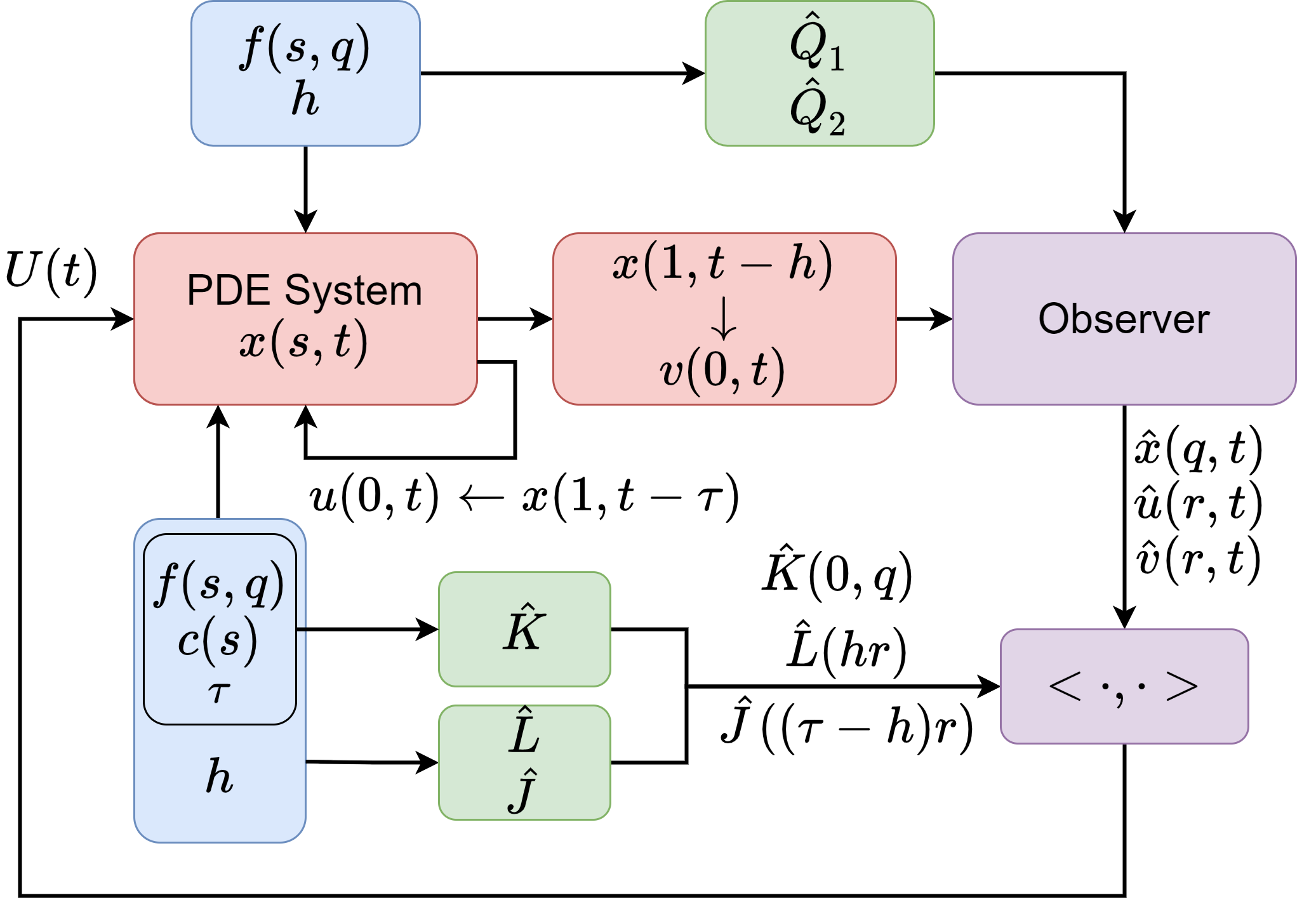
Figure 1: The neural operator learning framework for backstepping delay compensation control.

The following theorem establishes the exponentially stability for the cascading system under the output-feedback control with the DeepONets gains.

Theorem 6.11.

Consider the system (9)-(14), along with the observer (136)-(141) and the control (6), where the exact backstepping control kernels $K$, $L$, $J$ and observer gains $Q_{1}$, $Q_{2}$ are approximated by DeepONets $\hat{K}$, $\hat{L}$, $\hat{J}$ and $\hat{Q}_{1}$, $\hat{Q}_{2}$, respectively with the accuracy $\varepsilon\in(0,\varepsilon^{*})$. For any $(\tau,h,f,c)\in\mathbb{R}^{+}\times\mathbb{R}^{+}\times C^{1}(\mathcal{T}_{1})\times\underline{C}$ corresponding to the control kernels $K$, $L$, $J$, and $(h,f)\in\mathbb{R}^{+}\times C^{1}(\mathcal{T}_{1})$, corresponding to observer gains $Q_{1}$, $Q_{2}$, there exist a sufficiently small $\varepsilon^{*}>0$, such that the observer-based control (6) ensures that the observer cascading closed-loop system satisfies the exponential stability bound, for all $t>0$

$$\Theta(t)\leq W_{2}\mathrm{e}^{-\alpha_{2}t}\Theta(0),$$ (164)

where

$$\Theta(t)=\|x\|^{2}_{L^{2}}+\|v\|^{2}_{L^{2}}+\|u\|^{2}_{L^{2}}+\|\hat{x}\|^{2}_{L^{2}}+\|\hat{v}\|^{2}_{L^{2}}+\|\hat{u}\|^{2}_{L^{2}},$$

with $W_{2}>0$ and $\alpha_{2}>0$.

Proof 6.12.

We consider the observer error

$$\tilde{x}_{t}(s,t)= ~{}-\tilde{x}_{s}(s,t)+\int_{s}^{1}f(s,q)\tilde{x}(q,t)dq$$

$$~{}+c(s)\tilde{u}(0,t)-\hat{Q}_{1}(s)\tilde{v}(0,t),$$ (165)

$$\tilde{x}(0,t)= ~{}0,$$ (166)

$$h\tilde{v}_{t}(s,t)= ~{}\tilde{v}_{s}(s,t)-\hat{Q}_{2}(s)\tilde{v}(0,t),$$ (167)

$$\tilde{v}(1,t)= ~{}\tilde{x}(1,t),$$ (168)

$$\eta\tilde{u}_{t}(s,t)= ~{}\tilde{u}_{s}(s,t),$$ (169)

$$\tilde{u}(1,t)= ~{}0,$$ (170)

and the observer (136)-(141) with control (6), since they are equivalent to the cascading system (9)-(14) and observer (136)-(141) with control (6).

The proof contains two steps. First, we derive the target system of $(\hat{x},\hat{v},\hat{u})-(\tilde{x},\tilde{v},\tilde{u})$ by applying the backstepping transformation

$$\breve{z}(s,t)= ~{}\Gamma|_{\hat{K},\hat{L},\hat{J}}[\hat{x},\hat{v},\hat{u}](s,t),$$ (171)

$$\tilde{x}(s,t)= ~{}\mathcal{F}|_{F,M,P}[\tilde{z},\tilde{w}](s,t),$$ (172)

$$\tilde{v}(s,t)= ~{}\mathcal{R}|_{R}[\tilde{w}](s,t),$$ (173)

to transform the observer (136)-(141) cascading observer error system into the $(\breve{z},\hat{v},\hat{u})-(\tilde{z},\tilde{w},\tilde{u})$ system as

$$\breve{z}_{t}(s,t)= ~{}-\breve{z}_{s}(s,t)+\int_{s}^{1}\delta_{0}(s,q)\hat{x}(q,t)dq+\delta_{1}(s)\hat{v}(1,t)$$

$$~{}+\delta_{2}(s)\hat{u}(0,t)+\delta_{3}(s)\hat{v}(0,t)+G(s)\tilde{w}(0),$$ (174)

$$\breve{z}(0,t)= ~{}0,$$ (175)

$$h\hat{v}_{t}(r,t)= ~{}\hat{v}_{s}(r,t)+\hat{Q}_{2}(s)\tilde{w}(0,t),$$ (176)

$$\hat{v}(1,t)= ~{}\breve{z}(1,t)-h\int_{0}^{1}\tilde{L}(1+hs)\hat{v}(r)dr$$

$$~{}-\eta\int_{0}^{1}\tilde{J}(1+\eta s)\hat{u}(r)dr,$$ (177)

$$\eta\hat{u}_{t}(r,t)= ~{}\hat{u}_{s}(r,t),$$ (178)

$$\hat{u}(1,t)= ~{}v(0,t)=\hat{v}(0,t)+\tilde{w}(0,t),$$ (179)

$$\tilde{z}_{t}(s,t)= ~{}-\tilde{z}_{s}(s,t)+S(s)\tilde{u}(0,t)+\delta_{4}(s)\tilde{w}(0,t),$$ (180)

$$\tilde{z}(0,t)= ~{}0,$$ (181)

$$h\tilde{w}_{t}(s,t)= ~{}\tilde{w}_{s}(s,t)+\delta_{5}(s)\tilde{w}(0,t),$$ (182)

$$\tilde{w}(1,t)= ~{}\tilde{z}(1,t),$$ (183)

$$\eta\tilde{u}_{t}(s,t)= ~{}\tilde{u}_{s}(s,t),$$ (184)

$$\tilde{u}(1,t)= ~{}0,$$ (185)

where $\delta_{i}$, $i=0,...,3$ are given in (62)-(65) and

$$G(s)= ~{}\hat{Q}_{1}(s)-\int_{s}^{1}\hat{K}(s,q)\hat{Q}_{1}(q)dq-\frac{1}{h}\int_{0}^{1}\hat{L}(s+hr)dr$$

$$-\frac{1}{\eta}\hat{J}(s+\eta).$$ (186)

Since kernels $\hat{Q}_{1}$, $\hat{K}$, $\hat{L}$ and $\hat{J}$ are given bounded in Theorem 3.4, 5.7, and 5.9, $G(s)$ is also bounded, denoting the bound of $|G|$ by $\bar{G}$.

Second, we introduce the following Lyapunov functional to prove the stability of the cascading target system (174)-(185). Since target system (174)-(179) has the same form as that of the target system of the state-feedback system, except for one extra term in (174) and in (176), respectively, and boundary condition (179), we redefine the Lyapunov functionals (77)-(79) as follows:

$$V_{1} =\|\breve{z}^{2}\|^{2}_{L^{2}},~{}~{}V_{2}=\int_{0}^{1}\mathrm{e}^{-b_{1}s}\breve{z}^{2}(s,t)ds,$$ (187)

$$V_{3} =\|\hat{v}^{2}\|^{2}_{L^{2}},~{}~{}V_{4}=h\int_{0}^{1}\mathrm{e}^{b_{2}s}\hat{v}^{2}(s,t)ds,$$ (188)

$$V_{5} =\|\hat{u}^{2}\|^{2}_{L^{2}},~{}~{}V_{6}=\eta\int_{0}^{1}\mathrm{e}^{b_{3}s}\hat{u}^{2}(s,t)ds,$$ (189)

with $b_{i}>0$, $i=1,2,3$. Take time derivative of $V:=\beta_{1}V_{2}+\beta_{2}V_{4}+V_{6}+\beta_{5}V_{10}$ with $\beta_{i}>0$, $i=1,2,5$, we have

$$\dot{V}= -\beta_{1}\mathrm{e}^{-b_{1}}\breve{z}^{2}(1)-\beta_{1}b_{1}V_{2}+\beta_{2}\mathrm{e}^{b_{2}}\hat{v}^{2}(1)-\beta_{2}\hat{v}^{2}(0)$$

$$-\beta_{2}b_{2}V_{4}/h+2\beta_{1}\int_{0}^{1}\mathrm{e}^{-b_{1}s}\breve{z}(s)G(s)ds\tilde{w}(0)$$

$$+\mathrm{e}^{b_{3}}(\hat{v}(0)+\tilde{w}(0))^{2}+2\beta_{2}\int_{0}^{1}\mathrm{e}^{b_{2}s}\hat{v}(s)\hat{Q}_{2}(s)ds\tilde{w}(0)$$

$$-\hat{u}^{2}(0)+2\beta_{1}(I(t)+II(t)+III(t)+IV(t))$$

$$-b_{3}V_{6}/\eta+\beta_{5}\dot{V}_{10}.$$ (190)

where

$$I(t)= \int_{0}^{1}\int_{s}^{1}\mathrm{e}^{-b_{1}s}\breve{z}(s)\delta_{0}(s,q)\Gamma^{-1}|_{\hat{B},\hat{D},\hat{E}}[\breve{z},\hat{v},\hat{u}](q)dq,$$ (191)

$$II(t)= \int_{0}^{1}\mathrm{e}^{-b_{1}s}\breve{z}(s)\delta_{1}(s)ds\hat{v}(1),$$ (192)

$$III(t)= \int_{0}^{1}\mathrm{e}^{-b_{1}s}\breve{z}(s)\delta_{2}(s)ds\hat{u}(0),$$ (193)

$$IV(t)= \int_{0}^{1}\mathrm{e}^{-b_{1}s}\breve{z}(s)\delta_{3}(s)ds\hat{v}(0),$$ (194)

and combining (190), (85)-(87), we get

$$\dot{V}\leq -(\beta_{1}-3\beta_{2}\mathrm{e}^{b_{2}}-\beta_{1}\bar{\delta}_{1})\hat{z}^{2}(1)-(1-\beta_{1}\bar{\delta}_{3})\hat{u}^{2}(0)$$

$$-(\beta_{2}-3\mathrm{e}^{b_{3}}-\beta_{1}\bar{\delta}_{3})\hat{v}^{2}(0)-\beta_{1}\left[b_{1}-\bar{G}-\bar{\delta}_{1}\mathcal{O}(\varepsilon)\right.$$

$$\left.-\bar{\delta}_{0}\left(2\frac{\sqrt{\mathrm{e}^{b_{1}}}}{\sqrt{b_{1}}}(1+\bar{B})+\bar{D}+\bar{E}\right)-(\bar{\delta}_{1}+\bar{\delta}_{2}+\bar{\delta}_{3})\right]V_{2}$$

$$-\left[\beta_{2}b_{2}-\beta_{2}(\bar{Q}_{2}+\varepsilon)-\beta_{1}\bar{\delta}_{0}\bar{D}-\beta_{1}\bar{\delta}_{1}\mathcal{O}(\varepsilon)\right.$$

$$\left.~{}~{}~{}-3\beta_{2}h^{2}\mathrm{e}^{b_{2}}\mathcal{O}(\varepsilon^{2})\right]V_{4}/h$$

$$-\left[b_{3}-\beta_{1}\bar{\delta}_{0}\bar{E}-\beta_{1}\bar{\delta}_{1}\mathcal{O}(\varepsilon)-3\beta_{2}\eta^{2}\mathrm{e}^{b_{2}}\mathcal{O}(\varepsilon^{2})\right]V_{6}/\eta$$

$$+(\beta_{1}\bar{G}+\beta_{2}(\bar{Q}_{2}+\varepsilon)+2\mathrm{e}^{b_{3}})\tilde{w}^{2}(0)+\beta_{5}\dot{V}_{10}.$$ (195)

Let $\bar{\delta}_{i}=\mathcal{O}(\varepsilon)$, $i=1,...,5$ and recall (159),

$$\dot{V}\leq -(\beta_{1}-3\beta_{2}\mathrm{e}^{b_{2}}-\mathcal{O}(\varepsilon))\breve{z}^{2}(1)-(1-\mathcal{O}(\varepsilon))\hat{u}^{2}(0)$$

$$-(\beta_{2}-3\mathrm{e}^{b_{3}}-\mathcal{O}(\varepsilon))\hat{v}^{2}(0)-\beta_{1}(b_{1}-\bar{G}-\mathcal{O}(\varepsilon))V_{2}$$

$$-(\beta_{2}b_{2}-\mathcal{O}(\varepsilon))V_{4}/h-(b_{3}-\mathcal{O}(\varepsilon))V_{6}/\eta$$

$$-(\beta_{5}-\beta_{1}\bar{G}-\beta_{2}\bar{Q}_{2}-2\mathrm{e}^{b_{3}}-\mathcal{O}(\varepsilon))\tilde{w}^{2}(0)$$

$$-\beta_{5}(\beta_{3}\mathrm{e}^{-b_{4}}-\mathrm{e}^{b_{5}})\tilde{z}^{2}(1)$$

$$-\beta_{5}(\beta_{4}-\beta_{3}\bar{S})\tilde{u}^{2}(0)-\beta_{5}\beta_{3}(b_{4}-\bar{S}-\mathcal{O}(\varepsilon))V_{7}$$

$$-\frac{1}{h}\beta_{5}(b_{5}-\mathcal{O}(\varepsilon))V_{8}-\frac{1}{\eta}\beta_{5}\beta_{4}b_{6}V_{9},$$ (196)

Let $\beta_{2}=4\mathrm{e}^{b_{3}}$, $\beta_{1}=13\mathrm{e}^{b_{2}+b_{3}}$, $\beta_{3}=2\mathrm{e}^{b_{5}+b_{4}}$, $\beta_{4}=4\bar{S}\mathrm{e}^{b_{4}+b_{5}}$, $b_{1}=2\bar{G}$, $b_{4}=2\bar{S}$ and $\beta_{5}=2\beta_{1}\bar{G}+2\beta_{2}\bar{Q}_{2}+4\mathrm{e}^{b_{3}}=2\mathrm{e}^{b_{3}}(4\bar{G}+13\mathrm{e}^{b_{2}}\bar{Q}_{2}+2)$, which gives

$$\dot{V}\leq -(\mathrm{e}^{b_{2}+b_{3}}-\mathcal{O}(\varepsilon))\breve{z}^{2}(1)-(\mathrm{e}^{b_{3}}-\mathcal{O}(\varepsilon))\hat{v}^{2}(0)$$

$$-(1-\mathcal{O}(\varepsilon))\hat{u}^{2}(0)-13\mathrm{e}^{b_{2}+b_{3}}(\bar{G}-\mathcal{O}(\varepsilon))V_{2}$$

$$-(4b_{2}\mathrm{e}^{b_{3}}-\mathcal{O}(\varepsilon))V_{4}/h-(b_{3}-\mathcal{O}(\varepsilon))V_{6}/\eta$$

$$-\beta_{5}\phi V_{10}-(\mathrm{e}^{b_{3}}(4\bar{G}+13\mathrm{e}^{b_{2}}\bar{Q}_{2}+2)-\mathcal{O}(\varepsilon))\tilde{w}^{2}(0),$$

where $\phi=\min\{\bar{S}-\mathcal{O}(\varepsilon),\frac{b_{5}-\mathcal{O}}{h},\frac{b_{6}}{\eta}\}$. According to Theorem 1, there exists a small enough $\varepsilon^{*}$ such that

$$\dot{V}\leq \frac{1}{2}(-4\mathrm{e}^{b_{3}}\bar{G}V_{2}-13b_{2}\mathrm{e}^{b_{2}+b_{3}}V_{4}/h-b_{3}V_{6}/\eta)-\beta_{5}\phi V_{10}$$

$$\leq \alpha_{2}V,$$ (197)

where $\alpha_{2}=\frac{1}{2}\min\{4\mathrm{e}^{b_{3}}\bar{G},\frac{13b_{2}\mathrm{e}^{b_{2}+b_{3}}}{h},\frac{b_{3}}{\eta},\beta_{5}\}$.
Hence, $V\leq V(0)\mathrm{e}^{-\alpha_{2}t}$. Due to $L^{2}$ norm equivalence which are proven in Theorem 4.5 and 5.9, we conclude that there exist a positive constant $W_{2}$ such that (164) holds.

Throughout the stability analysis of the overall cascading system, the "separation principle" can also be proven.

7 Numerical Results: Full-State Feedback, Observer, and Output Feedback

7.1 Full-state feedback

We first solve equations (23)-(26) numerically by using the finite difference method to get datasets for different delays $\tau$, $h$ and different coefficient functions $f(s,q)$, $c(s)$ to train neural operators $\hat{\mathcal{K}}(\tau,f,c)$, $\hat{\mathcal{L}}(\tau,h,f,c)$ and $\hat{\mathcal{J}}(\tau,h,f,c)$. Let state delay $\tau\sim U(0.8,2)$, sensor delay $h\sim U(0.1,0.7)$, function $f(s,q)$ as a product of Chebyshev polynomials $f(s,q)=9\cos\big{(}\mu_{1}\cos^{-1}(s)\big{)}\cos\big{(}\mu_{2}\cos^{-1}(q)\big{)}$ with $\mu_{1},\mu_{2}\sim U(3,6)$, and function $c(s)$ as a Chebyshev polynomial $c(s)=\cos\big{(}\mu_{3}\cos^{-1}(s)\big{)}-\cos\big{(}\mu_{3}\cos^{-1}(1)\big{)}$ with $\mu_{3}\sim U(3,6)$, where $U(a,b)$ denotes the uniform distribution in the interval $[a,~{}b]$. In sampling, the discretized spatial step size is set to $\Delta s=0.02$. The Simulation code is shared on github.

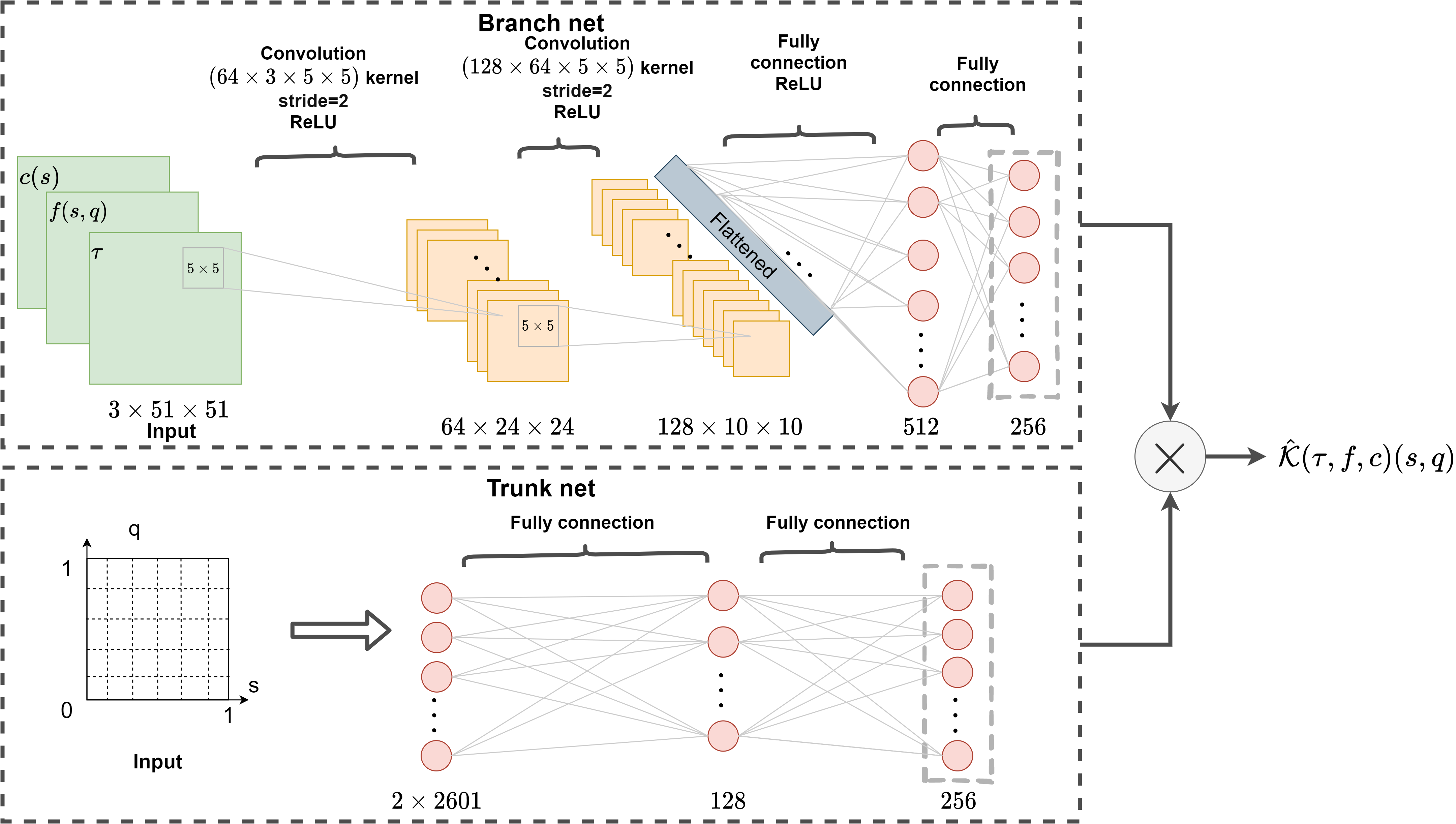
Figure 2: The DeepONet structure for kernel $K$.

As shown in Figure 2, we construct a branch net consisting of two layers $5\times 5$ convolutional neural networks (CNNs) with strides of $2$, and two layers of $12800\times 512$ and $512\times 256$ fully connected networks, and a trunk net consisting of two layers of $2601\times 128$ and $128\times 256$ fully connected networks. Being different from the neural network of $K$, the input to the neural networks of $L$ and $J$ is $4\times 51\times 51$. Three DeepONets are employed to learn the three kernel functions $K$, $L$ and $J$, which contain 6928641, 6930241 and 6930241 parameters, respectively. The loss function is chosen as the smooth $L_{1}$ [18], by using $\hat{\rho}\in\mathbb{R}$ to denote the prediction and $\rho\in\mathbb{R}$ to denote the true value:

$$\mathrm{Loss}(\hat{\rho}-\rho)=\left\{\begin{aligned} &0.5(\hat{\rho}-\rho)^{2},&\mathrm{if}~{}|\hat{\rho}-\rho|<1,\\ &|\hat{\rho}-\rho|-0.5,&\mathrm{otherwise.}\end{aligned}\right.$$ (198)

The smooth $L_{1}$ loss can be seen as exactly $L_{1}$ loss, but with the $|\hat{\rho}-\rho|$ portion replaced with a quadratic function such that its slope is $1$ at $|\hat{\rho}-\rho|=1$. The quadratic segment when $|\hat{\rho}-\rho|<1$ smooths the $L_{1}$ loss near $|\hat{\rho}-\rho|=0$, avoiding sharp changes in slope. The smooth $L_{1}$ combines the advantages of the $L_{1}$ and $L_{2}$ loss functions. When the difference between the prediction and the true value is large, the gradient value won’t be too large; when the difference between the prediction and the true value is small, the gradient value is also small. We also train the DeepONets using the $L_{2}$ loss function and find that using the smooth $L_{1}$ loss function exhibits better performance compared to the $L_{2}$ loss function. The evolution of loss over time of using both loss functions is shown in Figure 3, which illustrates that using the smooth $L_{1}$ loss has smaller errors and less fluctuations. Therefore, we will apply the smooth $L_{1}$ to train the networks. If not specifically pointed out, all the NNs in the following simulations are trained using the smooth $L_{1}$ loss function.

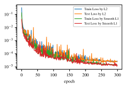
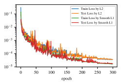
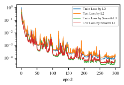
(a) $\mathrm{Loss}(\hat{K},K)$	(b) $\mathrm{Loss}(\hat{L},L)+\mathrm{Loss}(\hat{J},J)$	(c) $\mathrm{Loss}(\hat{Q}_{1},Q_{1})+\mathrm{Loss}(\hat{Q}_{2},Q_{2})$

Figure 3: (a) The loss of the neural control kernel for $K$. (b) The loss of the neural control kernels for $L$ and $J$. (c) The loss of neural observer gains.

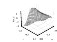
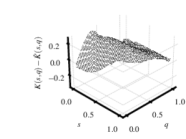
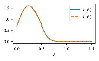
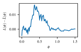
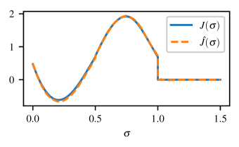
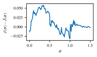
Figure 4: The first row shows the kernel functions $K(s,q)$, the learned kernel functions $\hat{K}(s,q)$ and the errors $K(s,q)-\hat{K}(s,q)$. The second row shows the kernel functions $L(s)$, the learned kernel functions $\hat{L}(\phi)$ and the errors $L(\phi)-\hat{L}(\phi)$. The last row shows the kernel functions $J(\sigma)$, the learned kernel functions $\hat{J}(\sigma)$ and the errors $J(\sigma)-\hat{J}(\sigma)$.

Since operator $\mathcal{K}$’s input variables are three and the other operators have four input variables, we first train $\hat{\mathcal{K}}(\tau,f,c)$ on a dataset of $8000$ numerical solutions with different parameters, and then train simultaneously the networks for operators $\hat{\mathcal{L}}(\tau,h,f,c)$ and $\hat{\mathcal{J}}(\tau,h,f,c)$ using $10000$ instances. The NN for operator $K$ achieves a training loss of $1.36\rm{E}-5$ and a testing loss of $1.34\rm{E}-5$ after $300$ epochs in around $11$ minutes, shown in Figure 3 (a). The two NNs for operator $L$ and $J$ achieve a training loss of $1.90\rm{E}-5$ and a testing loss of $1.90\rm{E}-5$ after $300$ epochs in about $15$ minutes, which are shown in Figure 3 (b). (The experimental code runs on Intel^® Core${}^{\text{TM}}$ i9-7900X CPU @ 3.30GHz $\times$ 20 and GPU TITAN Xp/PCle/SSE2.) In Figure 4, we demonstrate the analytical kernels that are solved numerically, the learned DeepONet kernels and the errors between them, where the coefficients are chosen as $\tau=1$, $h=0.5$, $f(s,q)$ with $\mu_{1}=\mu_{2}=5$ and $c(s)$ with $\mu_{3}=5$. Also, in Figure 5, we show both the analytical control gains and learned control gains, respectively.

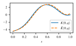
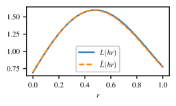
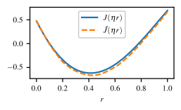
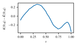
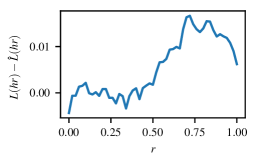
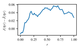
Figure 5: The first row shows the analyzed control gains $K(0,q)$, $L(hr)$, $J(\eta r)$, and the learned control gains $\hat{K}(0,q)$, $\hat{L}(hr)$, $\hat{J}(hr)$. The last row shows the errors $K_{1}(0,q)-\hat{K}_{1}(0,q)$, $L(hr)-\hat{L}(hr)$, $J(\eta r)-\hat{J}(\eta r)$.

To test the performance of the neural operator based control, we apply the trained neural gains in controller (4.5). Here, we use the same parameter settings as Figure 4 and let initial condition be $x(s,0)=\sin(x)$. The upwind scheme with a time step size of $\Delta t=0.001$ and a trapezoidal integration rule are used to numerically solve the PIDE under controller (4.5). Before proceeding, we show in Figure 6 that the dynamical state $x(s,t)$ of the system under a nominal controller without delay compensation fails to converge.

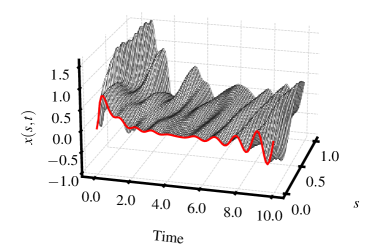
Figure 6: The system dynamics without delay compensation.

In Figure 7, we demonstrate the dynamics of the closed-loop with the full state feedback, using the numerically solved control gains and the DeepONet learned control gains, respectively. The closed-loop system dynamics with NO kernels approximates the PDE well with a peak error of less than $8\%$ compared to the closed-loop system with analytical kernels.

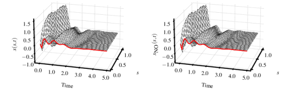
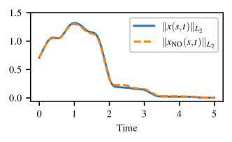
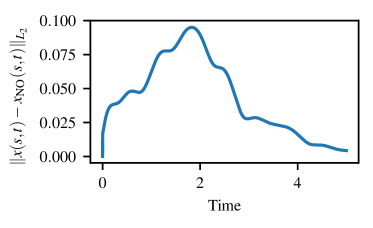
Figure 7: The closed-loop evolution with full-state feedback (4.5). The left column in the first row shows state $x(s,t)$ with the analyzed kernels $K$, $L$ and $J$. The right column in the first row shows state $x_{\mathrm{NO}}(s,t)$ with the learned kernels $\hat{K}$, $\hat{L}$ and $\hat{J}$. The last row shows the $L_{2}$-norm of state $x$, $x_{\mathrm{NO}}$, and the error between them.

7.2 Output feedback

We train two neural observer gains $\hat{Q}_{1}(s)$ and $\hat{Q}_{2}(s)$ instead of the four observer kernels, which reduces the computational cost in half. The same parameter settings as for the full-state feedback are applied in the NN training, and the sensor delay $h$ is chosen from $U(0.1,0.6)$. Similar to the DeepONets for learning control kernels, except that the input channel for the first layer CNN is $2$. Two DeepONets are employed to learn the gain functions $Q_{1}$ and $Q_{2}$, respectively, each containing $6926913$ parameters. The two observer networks are trained together on $1600$ instances, which only takes around 4 minutes. Figure 8 shows the analyzed observer gains, the learned DeepONet observer gains and the errors between them as $h=0.5s$. The network achieves a training loss of $5.02\rm{E}-5$ and a testing loss of $6.36\rm{E}-5$ after $300$ epochs, which are shown in Figure 3 (c).

Figure 9 demonstrates the convergence of the observation with the DeepONets learned gains to the system’s actual state. In Figure 10, we test the closed-loop system under the output feedback (6) with three DeepONets approximating the control kernels and two DeepONets approximating the observer gains when the initial condition of the observer is set to the initial value of the system plus a random number that obeys $U(-1,1)$.

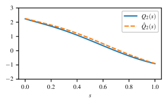
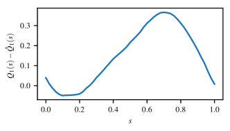
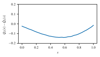
Figure 8: The first row shows the analyzed observer gains $Q_{1}(s)$, $Q_{2}(s)$, and the learned observer gains $\hat{Q}_{1}(s)$, $\hat{Q}_{2}(s)$. The last row shows the error $Q_{1}(s)-\hat{Q}_{1}(s)$, $Q_{2}(s)-\hat{Q}_{2}(s)$.

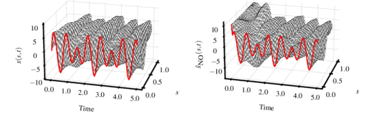
Figure 9: The system actual state $x(s,t)$ and the neural operator based observer $\hat{x}_{\mathrm{NO}}(s,t)$ under controller $U(t)=5\sin(3\pi t)+3\cos(2\pi t)$. The left column showcases the actual state of the system state. The right column showcases the estimated system state $\hat{x}_{\mathrm{NO}}(s,t)$ with the neural operator based observer. Note that the initial condition of the system is $x(s,0)=\sin(2\pi s)$, while the initial condition of the neural operator observers is $\hat{x}_{\mathrm{NO}}(s,0)=10$.

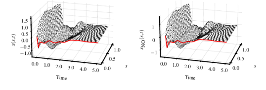
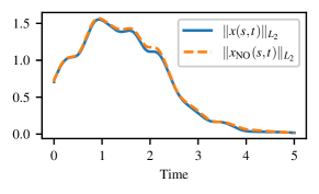
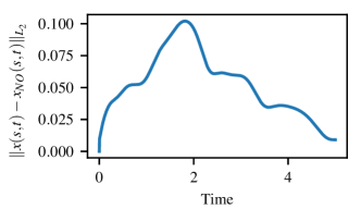
Figure 10: The closed-loop evolution under output feedback. The left column in the fist row showcases the evolution of state $x(s,t)$ with the analytical kernels $K$, $L$, $J$ and observer gains $Q_{1}$, $Q_{2}$. The right column in the first row showcases the evolution of state $x_{\mathrm{NO}}(s,t)$ with NO kernels $\hat{K}$, $\hat{L}$, $\hat{J}$ and NO observer gains $\hat{Q}_{1}$, $\hat{Q}_{2}$. The last row shows the $L_{2}$-norm of state $x$, $x_{\mathrm{NO}}$, and the error between them.

Table 1: Summary of kernel function calculation time consumption.

	Model	Average Calculation Time (sec) (spatial step size $\Delta s=0.02$)	Average Calculation Time (sec) (spatial step size $\Delta s=0.01$)	Average Calculation Time (sec) (spatial step size $\Delta s=0.005$)
Control kernels ($K$, $L$, $J$)	Numerical solver	0.025	0.654	1.692
	Neural operators	0.011	0.0139	0.0265
	Speedups	$2.3\times$	$47.1\times$	$63.8\times$
Observer gains ($Q_{1}$, $Q_{2}$)	Numerical solver	0.030	0.079	0.348
	Neural operators	0.006	0.006	0.007
	Speedups	$5\times$	$13.2\times$	$49.7\times$

Table 1 lists the time consumption of kernel functions solved numerically and generated by the trained DeepONets, respectively. The time taken by the numerical solvers will increase dramatically as the discrete spatial step size increases, which implies sampling precision increasing. In contrast, the computation time of the NOs increases only slightly as the spacial step size increases, but both the loss of the control kernels and observer gains remains on the order of $10^{-5}$. We use root mean square error (RMSE) to measure the approximation accuracy, which reflects the true magnitude of the error. RMSE can be written as a function of loss function (198):

$$\mathrm{RMSE}(\hat{\rho}-\rho)=\left\{\begin{aligned} &\sqrt{2\mathrm{Loss}(\hat{\rho}-\rho)},&\mathrm{if}~{}|\hat{\rho}-\rho|<1,\\ &\mathrm{Loss}(\hat{\rho}-\rho)+0.5,&\mathrm{otherwise.}\end{aligned}\right.$$ (199)

Hence, the accuracy of the control kernels is on the order of $10^{-3}$ and the observer gains on the order of $10^{-2}$, which are calculated from the loss values of the NNs according to (199).

8 Conclusion

In this paper, we apply the DeepONet operators to learn the PDE backstepping control kernels and observer of a first-order hyperbolic PIDE system with state and sensor delays. Three neural operators are trained for the state feedback control from a group of numerical solutions of the backstepping kernel equations, which approximate three control kernel functions with the accuracy of magnitude of $10^{-3}$. The existence of arbitrary-precision NOs’ approximation of the analytical kernel operators is proved by using the universal approximation theorem. The stability of the closed-loop system under state feedback with NO learning gains is also proved. Moreover, we use two neural operators to learn the observer gains and prove the observer with neural gains converge. The simulation results show that the accuracy of observer gains approximation can reach the magnitude of $10^{-2}$. Combined with the observer based control system and observer error system, the stability of the output feedback system is proved, which verifies the separation principle under the neural operator gains. Further research will concern the delay-adaptive control of PDEs whose delays are unknown and control of high-dimensional PDEs control whose kernel functions are defined in higher spatial dimension.

References

- Aamo [2015] Aamo, O.M., 2015. Leak detection, size estimation and localization in pipe flows. IEEE Transactions on Automatic Control 61, 246–251.
- Abate et al. [2020] Abate, A., Ahmed, D., Giacobbe, M., Peruffo, A., 2020. Formal synthesis of lyapunov neural networks. IEEE Control Systems Letters 5, 773–778.
- Anfinsen and Aamo [2022] Anfinsen, H., Aamo, O.M., 2022. Leak detection, size estimation and localization in branched pipe flows. Automatica 140, 110213.
- Auriol et al. [2018a] Auriol, J., Aarsnes, U., Martin, P., Di Meglio, F., 2018a. Delay-robust control design for two heterodirectional linear coupled hyperbolic PDEs. IEEE Transactions on Automatic Control 63, 3551–3557.
- Auriol et al. [2018b] Auriol, J., Bribiesca-Argomedo, F., Saba, D., Loreto, M.D., Di Meglio, F., 2018b. Delay-robust stabilization of a hyperbolic PDE-ODE system. Automatica 95, 494–502.
- Bastin et al. [2019] Bastin, G., Coron, J.M., Hayat, A., Shang, P., 2019. Boundary feedback stabilization of hydraulic jumps. IFAC Journal of Systems and Control 7, 100026.
- Bhan et al. [2023a] Bhan, L., Shi, Y., Krstic, M., 2023a. Neural operators for bypassing gain and control computations in PDE backstepping. arXiv preprint arXiv:2302.14265 .
- Bhan et al. [2023b] Bhan, L., Shi, Y., Krstic, M., 2023b. Operator learning for nonlinear adaptive control, in: Learning for Dynamics and Control Conference, PMLR. pp. 346–357.
- Chen et al. [2019] Chen, C., Chen, X.Q., Ma, F., Zeng, X.J., Wang, J., 2019. A knowledge-free path planning approach for smart ships based on reinforcement learning. Ocean Engineering 189, 106299.
- Chen and Chen [1995] Chen, T., Chen, H., 1995. Universal approximation to nonlinear operators by neural networks with arbitrary activation functions and its application to dynamical systems. IEEE transactions on neural networks 6, 911–917.
- Chu et al. [2022] Chu, N.H., Hoang, D.T., Nguyen, D.N., Van Huynh, N., Dutkiewicz, E., 2022. Joint speed control and energy replenishment optimization for UAV-assisted iot data collection with deep reinforcement transfer learning. IEEE Internet of Things Journal 10, 5778–5793.
- Coron et al. [2013] Coron, J., Vazquez, R., Krstic, M., Bastin, G., 2013. Local exponential stabilization of a quasilinear hyperbolic system using backstepping. SIAM Journal on Control and Optimization 51, 2005–2035.
- Deng et al. [2022] Deng, B., Shin, Y., Lu, L., Zhang, Z., Karniadakis, G.E., 2022. Approximation rates of deeponets for learning operators arising from advection–diffusion equations. Neural Networks 153, 411–426.
- Di Meglio et al. [2018] Di Meglio, F., Argomedo, F.B., Hu, L., Krstic, M., 2018. Stabilization of coupled linear heterodirectional hyperbolic PDE–ODE systems. Automatica 87, 281–289.
- Di Meglio et al. [2013] Di Meglio, F., Vazquez, R., Krstic, M., 2013. Stabilization of a system of coupled first-order hyperbolic linear PDEs with a single boundary input. IEEE Transactions on Automatic Control 58, 3097–3111.
- Dogru et al. [2022] Dogru, O., Velswamy, K., Ibrahim, F., Wu, Y., Sundaramoorthy, A.S., Huang, B., Xu, S., Nixon, M., Bell, N., 2022. Reinforcement learning approach to autonomous PID tuning. Computers & Chemical Engineering 161, 107760.
- Garcıa and Fernández [2015] Garcıa, J., Fernández, F., 2015. A comprehensive survey on safe reinforcement learning. Journal of Machine Learning Research 16, 1437–1480.
- Girshick [2015] Girshick, R., 2015. Fast R-CNN, in: Proceedings of the IEEE international conference on computer vision, pp. 1440–1448.
- Götz and Perera [2010] Götz, T., Perera, S., 2010. Optimal control of melt-spinning processes. Journal of Engineering Mathematics 67, 153–163.
- Hambly et al. [2021] Hambly, B., Xu, R., Yang, H., 2021. Policy gradient methods for the noisy linear quadratic regulator over a finite horizon. SIAM Journal on Control and Optimization 59, 3359–3391.
- He and Ge [2015] He, W., Ge, S.S., 2015. Dynamic modeling and vibration control of a flexible satellite. IEEE Transactions on Aerospace and Electronic Systems 51, 1422–1431.
- He et al. [2018] He, W., He, X., Zou, M., Li, H., 2018. PDE model-based boundary control design for a flexible robotic manipulator with input backlash. IEEE Transactions on Control Systems Technology 27, 790–797.
- Hu et al. [2015] Hu, L., Di Meglio, F., Vazquez, R., Krstic, M., 2015. Control of homodirectional and general heterodirectional linear coupled hyperbolic PDEs. IEEE Transactions on Automatic Control 61, 3301–3314.
- Jiang et al. [2020] Jiang, Z.P., Bian, T., Gao, W., et al., 2020. Learning-based control: A tutorial and some recent results. Foundations and Trends® in Systems and Control 8, 176–284.
- Krstic et al. [2023] Krstic, M., Bhan, L., Shi, Y., 2023. Neural operators of backstepping controller and observer gain functions for reaction-diffusion PDEs. arXiv preprint arXiv:2303.10506 .
- Krstic and Smyshlyaev [2008] Krstic, M., Smyshlyaev, A., 2008. Backstepping boundary control for first order hyperbolic PDEs and application to systems with actuator and sensor delays. System and Control Letters 57, 750–758.
- Lawrence et al. [2022] Lawrence, N.P., Forbes, M.G., Loewen, P.D., McClement, D.G., Backström, J.U., Gopaluni, R.B., 2022. Deep reinforcement learning with shallow controllers: An experimental application to PID tuning. Control Engineering Practice 121, 105046.
- Li et al. [2021] Li, B., Yang, Z.p., Chen, D.q., Liang, S.y., Ma, H., 2021. Maneuvering target tracking of UAV based on MN-DDPG and transfer learning. Defence Technology 17, 457–466.
- Lu et al. [2019] Lu, L., Jin, P., Karniadakis, G.E., 2019. Deeponet: Learning nonlinear operators for identifying differential equations based on the universal approximation theorem of operators. arXiv preprint arXiv:1910.03193 .
- Mavkov et al. [2017] Mavkov, B., Witrant, E., Prieur, C., 2017. Distributed control of coupled inhomogeneous diffusion in tokamak plasmas. IEEE Transactions on Control Systems Technology 27, 443–450.
- McClement et al. [2022] McClement, D.G., Lawrence, N.P., Backström, J.U., Loewen, P.D., Forbes, M.G., Gopaluni, R.B., 2022. Meta reinforcement learning for adaptive control: An offline approach. submitted to Journal of Process Control .
- Mohammadi et al. [2021] Mohammadi, H., Zare, A., Soltanolkotabi, M., Jovanović, M.R., 2021. Convergence and sample complexity of gradient methods for the model-free linear–quadratic regulator problem. IEEE Transactions on Automatic Control 67, 2435–2450.
- Nguyen et al. [2021] Nguyen, H.H., Zieger, T., Braatz, R.D., Findeisen, R., 2021. Robust control theory based stability certificates for neural network approximated nonlinear model predictive control. IFAC-PapersOnLine 54, 347–352.
- O’Connell et al. [2022] O’Connell, M., Shi, G., Shi, X., Azizzadenesheli, K., Anandkumar, A., Yue, Y., Chung, S.J., 2022. Neural-fly enables rapid learning for agile flight in strong winds. Science Robotics 7, eabm6597.
- Qi et al. [2021] Qi, J., Dubljevic, S., Kong, W., 2021. Output feedback compensation to state and measurement delays for a first-order hyperbolic PIDE with recycle. Automatica 128, 109565.
- Qi et al. [2022] Qi, J., Mo, S., Krstic, M., 2022. Delay-compensated distributed PDE control of traffic with connected/automated vehicles. IEEE Transactions on Automatic Control 68, 2229–2244.
- Qin et al. [2021] Qin, Z., Chen, Y., Fan, C., 2021. Density constrained reinforcement learning, in: International Conference on Machine Learning, PMLR. pp. 8682–8692.
- Soloperto et al. [2018] Soloperto, R., Müller, M.A., Trimpe, S., Allgöwer, F., 2018. Learning-based robust model predictive control with state-dependent uncertainty. IFAC-PapersOnLine 51, 442–447.
- Vazquez and Krstic [2016] Vazquez, R., Krstic, M., 2016. Boundary control of coupled reaction-advection-diffusion systems with spatially-varying coefficients. IEEE Transactions on Automatic Control 62, 2026–2033.
- Vazquez et al. [2023] Vazquez, R., Zhang, J., Qi, J., Krstic, M., 2023. Kernel well-posedness and computation by power series in backstepping output feedback for radially-dependent reaction–diffusion PDEs on multidimensional balls. Systems & Control Letters 177, 105538.
- Venturini et al. [2021] Venturini, F., Mason, F., Pase, F., Chiariotti, F., Testolin, A., Zanella, A., Zorzi, M., 2021. Distributed reinforcement learning for flexible and efficient uav swarm control. IEEE Transactions on Cognitive Communications and Networking 7, 955–969.
- Wang and Krstic [2020] Wang, J., Krstic, M., 2020. Delay-compensated control of sandwiched ODE–PDE–ODE hyperbolic systems for oil drilling and disaster relief. Automatica 120, 109131.
- Wang and Krstic [2022] Wang, J., Krstic, M., 2022. Event-triggered output-feedback backstepping control of sandwich hyperbolic PDE systems. IEEE Transactions on Automatic Control 67, 220–235. doi:10.1109/TAC.2021.3050447.
- Wang et al. [2021] Wang, N., Gao, Y., Zhang, X., 2021. Data-driven performance-prescribed reinforcement learning control of an unmanned surface vehicle. IEEE Transactions on Neural Networks and Learning Systems 32, 5456–5467.
- Xu and Dubljevic [2018] Xu, X., Dubljevic, S., 2018. Optimal tracking control for a class of boundary controlled linear coupled hyperbolic PDE systems: Application to plug flow reactor with temperature output feedback. European Journal of Control 39, 21–34.
- Yu et al. [2022] Yu, H., Auriol, J., Krstic, M., 2022. Simultaneous downstream and upstream output-feedback stabilization of cascaded freeway traffic. Automatica 136, 110044.
- Zhang et al. [2022] Zhang, S., Li, Y., Dong, Q., 2022. Autonomous navigation of uav in multi-obstacle environments based on a deep reinforcement learning approach. Applied Soft Computing 115, 108194.
- Zhang et al. [2020] Zhang, Y., Vuong, Q., Ross, K., 2020. First order constrained optimization in policy space. Advances in Neural Information Processing Systems 33, 15338–15349.
- Zheng et al. [2023] Zheng, Y., Tao, J., Hartikainen, J., Duan, F., Sun, H., Sun, M., Sun, Q., Zeng, X., Chen, Z., Xie, G., 2023. DDPG based LADRC trajectory tracking control for underactuated unmanned ship under environmental disturbances. Ocean Engineering 271, 113667.
- Zhou et al. [2022] Zhou, R., Quartz, T., De Sterck, H., Liu, J., 2022. Neural lyapunov control of unknown nonlinear systems with stability guarantees. Advances in Neural Information Processing Systems 35, 29113–29125.