An Analysis of Multi-Agent Reinforcement Learning for Decentralized Inventory Control Systems

Abstract

Most solutions to the inventory management problem assume a centralization of information that is incompatible with organisational constraints in real supply chain networks. The inventory management problem is a well-known planning problem in operations research, concerned with finding the optimal re-order policy for nodes in a supply chain. While many centralized solutions to the problem exist, they are not applicable to real-world supply chains made up of independent entities. The problem can however be naturally decomposed into sub-problems, each associated with an independent entity, turning it into a multi-agent system. Therefore, a decentralized data-driven solution to inventory management problems using multi-agent reinforcement learning is proposed where each entity is controlled by an agent. Three multi-agent variations of the proximal policy optimization algorithm are investigated through simulations of different supply chain networks and levels of uncertainty. The centralized training decentralized execution framework is deployed, which relies on offline centralization during simulation-based policy identification, but enables decentralization when the policies are deployed online to the real system. Results show that using multi-agent proximal policy optimization with a centralized critic leads to performance very close to that of a centralized data-driven solution and outperforms a distributed model-based solution in most cases while respecting the information constraints of the system.

[inst1]organization=Sargent Centre for Process Systems Engineering,addressline=Department of Chemical Engineering, Imperial College London, city=London, postcode=SW7 2AZ, country=United Kingdom

[inst2]organization=Centre for Process Integration,addressline=Department of Chemical Engineering, The University of Manchester, Manchester, city=Manchester, postcode=M13 9PL, country=United Kingdom

1 Introduction

1.1 An overview of supply chain management and uncertainty

Production planning, inventory control and transportation form key decision functions within industrial production systems. These functions identify decisions that define production targets, as well as maintain and transport material inventory, across multiple distributed production facilities (i.e. echelons) to transform raw materials into marketable products. These decisions may be continuous or discrete depending on the decision function, and as a result, these problems are formulated either as either linear programming (LP) or mixed-integer linear programming (MILP). Indeed, exact optimization approaches underpin the current state-of-the-art for industrial scale problems (Grossmann et al., 2016).

However, these decision problems are uncertain, with the associated random variables either exogenous or endogenous in nature. In multi-echelon inventory control problems, common respective examples include customer demand at the retailer and production lead times (Song et al., 2017). To mitigate phenomena such as the bull-whip effect (Lee et al., 2004) in inventory control problems, decision-making should be coordinated across the supply chain and account for uncertainty. A number of stochastic (Hamdan and Diabat, 2019), robust (Aharon et al., 2009) and distributionally-robust (Hashemi-Amiri et al., 2023) mathematical programming formulations have been proposed to account for distributional, set-based, and ambiguity set descriptions of uncertain parameters, respectively. Despite providing principled frameworks to account for uncertainty, stochastic and distributionally-robust approaches face issues related to online tractability, with robust formulations known to introduce conservatism, when applied within receding-horizon frameworks.

1.2 Reinforcement Learning and multi-echelon inventory control

More recently, there has been interest in the development of Reinforcement Learning (RL) solutions to multi-echelon inventory control problems (Boute et al., 2022). Closely connected to dynamic programming (DP), RL has been demonstrated as a general solution method for identifying approximately optimal parametric policy functions for stochastic decision processes. This is primarily because parametric RL policies aim to satisfy the Bellman optimality equation (Powell, 2007; Bhandari and Russo, 2019) with optimal policy parameters identified through iterative model-free updates (e.g. via the policy gradient theorem) (Levine et al., 2020). This process can be thought of as a noisy search process. In principle, it could be conducted online (Lawrence et al., 2022), but for the purpose of safety and sample efficiency preference is for identification to utilize offline simulation of an approximate model typically with distributional descriptions of uncertain parameters (Mowbray et al., 2022). This enables the cheap generation of near-optimal online management decisions by the inference process of the policy function approximation. This is a major benefit relative to mathematical programming approaches that require resolving an optimization problem recursively in a receding or shrinking horizon framework. This requirement often means that, for example, stochastic mathematical programming models have to make significant approximation to uncertain parameters described by large or continuous support in order satisfy time constraints imposed on the identification of a decision.

Based on the promise of RL, a number of preliminary studies have been conducted. For example, Hubbs et al. (2020) demonstrated the application of the proximal policy optimization (PPO) algorithm on a multi-echelon inventory control problem subject to demand uncertainty and integer constraints on reorder decisions. The algorithm was demonstrated to outperform a MILP strategy with nominal demand data. Wu et al. (2023) provided a derivative-free optimization approach to RL together with a flexible, risk-sensitive formulation. The method was benchmarked to the work provided in Hubbs et al. (2020) and demonstrated an 11% improvement in expected performance for the same computational budget. Perez et al. (2021) extended this analysis for continuous reorder decisions and benchmarked against nominal and multi-stage stochastic linear programming formulations under the assumption of demand uncertainty at the retailer.

In general, these investigations demonstrated that the RL methods were competitive with but outperformed by benchmark mathematical programming formulations. However, although these works provide an excellent investigation of RL, they consider supply chain instances with sequential structure, relatively few production echelons, and make two important assumptions. Firstly, production processes and transportation times are jointly approximated via a deterministic safety lead time. This is to overcome the computational barriers of integrating the description of planning, production, and transportation into one model and is a common assumption in constructing supply chain management policies (Lejarza et al., 2022). However, the rationale for describing lead time as a random variable has long been documented. For example, Nevison and Burstein (1984) presented a DP approach to single-product, single-echelon inventory control under exogenous production lead times and deterministic demand. It should be noted that the application of DP necessitates a relatively simple problem instance with small control and state sets. Song et al. (2017) characterize the optimal reorder policy for a single product, single-echelon dual-sourcing problem, but with endogenous lead time uncertainty.

For larger industrial problems, similar reasoning processes to that provided in Song et al. (2017) become very difficult and reliant on advanced computational tools. Thevenin et al. (2022) proposed a robust optimization approach to identify a multi-period single-echelon inventory reorder policy subject to lead time uncertainty and multi-sourcing (i.e. with at least two or more potential suppliers). Liu et al. (2021) proposed a two-stage, distributionally robust model to handle uncertainty in transportation times for large-scale maritime inventory routing problems. The authors demonstrate that a tailored multi-cut bender’s decomposition algorithm can exploit structure in the resultant model to reduce the computation required to identify a solution. Franco and Alfonso-Lizarazo (2020) proposed a stochastic formulation considering lead time uncertainty for inventory control of multiple pharmaceutical products within a hospital. The policy derived from the methodology provides a performance improvement of 15% to that currently implemented by the hospital subject to the case study. However, as reviewed in Ben-Ammar et al. (2022) and highlighted in Franco and Alfonso-Lizarazo (2020), it is rare that lead time uncertainty is accounted for in the literature. To the author’s knowledge, only two works detailed by Gijsbrechts et al. (2022) and Madeka et al. (2022) consider the impact of stochastic lead times on parametric inventory control policy approximations. However, analysis in both is specific to single-echelon inventory control problems.

The second assumption of previous works examining the use of RL is that information can be centralized for the purposes of decision-making in real-time to enable closed-loop decision-making. As the scale of the system increases, this assumption will become more difficult to satisfy in practice, primarily because the nature of production is inherently distributed (Andersson and Marklund, 2000; Ghasemi et al., 2022), but also due to information sharing constraints often observed in multi-stage production systems (Sahin and Robinson, 2002). This has led to an interest in the development of decentralized decision-making frameworks.

1.3 Decentralized decision-making and multi-echelon inventory control

Two class of methods that could reduce dependence on the latter assumption is distributed optimization and multi-agent RL (MARL). The use of distributed optimization approaches for inventory control has been well described elsewhere (Dunbar and Desa, 2017; Fu et al., 2020). A major comparative benefit of MARL approaches is that they inherit flexibility in the treatment of sources of uncertainty associated with single agent RL and other simulation-based approaches, but enable the decentralization of collaborative decision-making in deployment, without the requirements for coordinated computation online. Multiple agents hold independent parametric policies, which are each conditioned on a local, partial state observation to provide a decentralized joint policy. This means the state information does not need to be shared between production echelons online. As a result, MARL provides an opportunity to coordinate decision-making in a decentralized manner, whilst respecting information-sharing constraints online. Instead, multi-agent coordination is provided during policy identification, which is conducted offline. This is highlighted by Fig. 1.

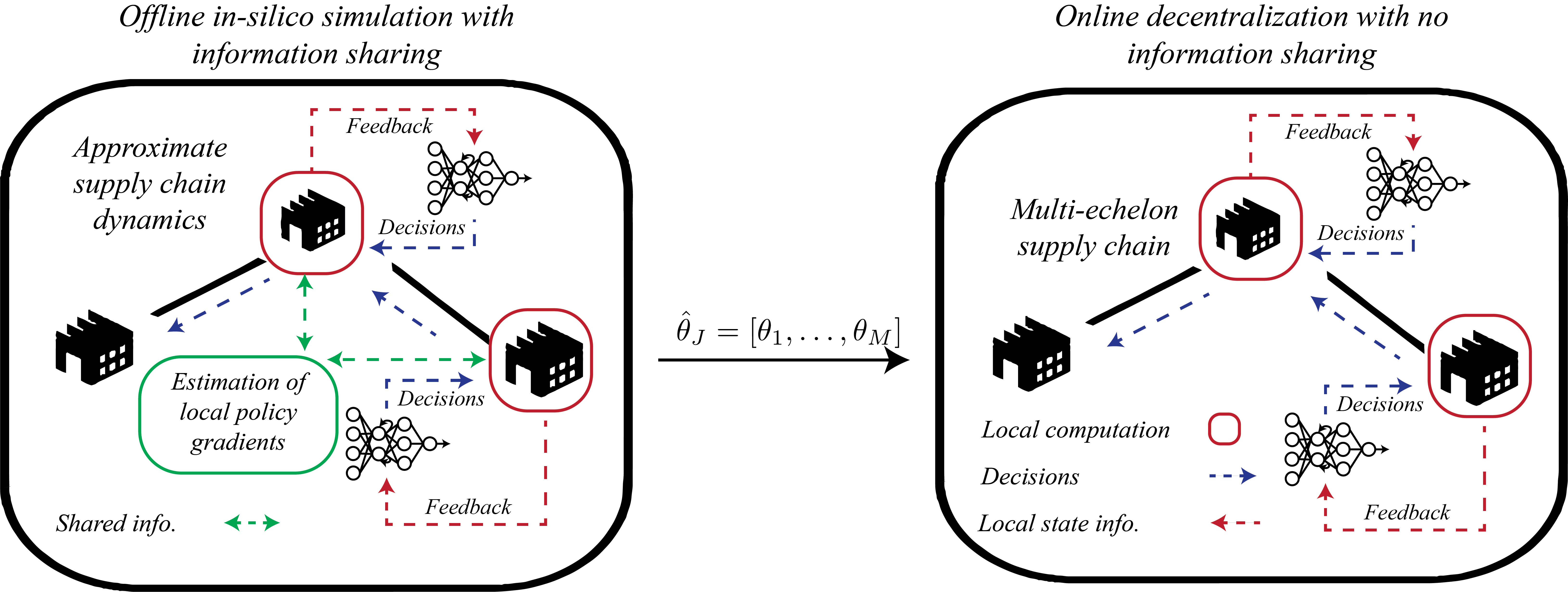
Figure 1: A framework for coordinating multi-agent reinforcement learning policies offline, enabling complete decentralization of decision-making online, through transfer of policy parameters, $\hat{\theta}_{J}$

To the authors’ knowledge, multi-agent RL has been explored by two previous investigations. The first explored planning and management problems involving multiple independent entities operating with deterministic retailer demand and lead-times (Fuji et al., 2018). The second work focused on the examination of MARL performance in serial supply chains, with backlog, dual-sourcing, and lost sales under stochastic demand with benchmark to commonly used heuristic re-order policies (Liu et al., 2022). While MARL is powerful, the associated algorithms are characterized by many hyperparameters and different amounts of information sharing in policy identification. Further, MARL does not generally have the stability, safety and feasibility guarantees observed in traditional optimal control methods such as model predictive control (MPC) (Görges, 2017). This has slowed the adoption of MARL methods to control large real-world systems.

1.4 Motivation

In this work, we provide a thorough interrogation of MARL methods and their performance in single-product, multi-echelon inventory control problems characterized by different production network structures, sizes, and sources of uncertainty (i.e. both demand and lead time uncertainty). We explore the effects of varying degrees of information centralization in policy identification and benchmark the resultant joint policy performance to a distributed optimization approach utilizing nominal descriptions of uncertain variables. In doing so, we develop on previous works that have provided preliminary but limited interrogation of these algorithms. We provide comments on the potential application of MARL methods in practice and scope for future work.

2 Problem Description

2.1 Mathematical Formulation

The IM problem can be formulated as a constrained optimization problem. The discrete-time formulation is considered here, where the aim of the optimization is to find the optimal re-order quantity at each node $m$ and each time period $t$ for all $M$ nodes over a fixed horizon of $T$ time periods. This can be written as:

$$\begin{split}\scriptscriptstyle&\max\sum_{m=1}^{M}\sum_{t=1}^{T}P^{m}s_{r}^{m}[t]-C^{m}o_{r}^{m}[t]-I^{m}i^{m}[t]-B^{m}b^{m}[t]\,,\end{split}$$ (1a)

$$\begin{split}&\text{subject to}\end{split}$$

$$\begin{split}&i^{m}[t]=i_{0}^{m}[t]-s_{r}^{m}[t]+a_{r}^{m}[t]\,,\quad\forall m,\forall t,\end{split}$$ (1b)

$$\begin{split}&b^{m_{d}}[t]=b_{0}^{m_{d}}[t]-s_{r}^{m_{d}}[t]+d_{r}^{m_{d}}[t],\quad\forall m,\forall d\in\mathcal{D}_{m}\,,\end{split}$$ (1c)

$$\begin{split}&s_{r}^{m_{d}}[t]\leq b_{0}^{m_{d}}[t]+d_{r}^{m_{d}}[t]\,,\quad\forall m,\forall t,\forall d\in\mathcal{D}_{m}\end{split}$$ (1d)

$$\begin{split}&s_{r}^{m}[t]\leq i_{0}^{m}[t]+a_{r}^{m}[t],\quad\forall m,\forall t,\end{split}$$ (1e)

$$\begin{split}&a_{r}^{m}[t]=s_{r}^{m_{u}}[t-\tau_{r}^{m}],\quad\forall m\neq 1\,,t\geq\tau_{r}^{m}\end{split}$$ (1f)

$$\begin{split}&a_{r}^{1}[t]=o_{r}^{1}[t-\tau_{r}^{1}],\quad t\geq\tau_{r}^{1}\end{split}$$ (1g)

$$\begin{split}&d_{r}^{m_{d}}=o_{r}^{d},\quad\forall m,\forall d\in\mathcal{D}_{m}\,,\end{split}$$ (1h)

$$\begin{split}&\text{with}\end{split}$$

$$\begin{split}&d_{r}^{m}[t]=c^{m}[t],\quad\forall m\in\mathcal{C},\forall t\end{split}$$ (1i)

$$\begin{split}&o_{r}^{m}[t]\leq O_{r_{\max}}^{m}\,,i^{m}[t]\leq I_{\max}^{m}\,,\quad\forall m,\forall t,\end{split}$$ (1j)

where $s_{r}$ is the sales/amount of goods shipped to a downstream node (or customers), $o_{r}$ is the replenishment order, $d_{r}$ is demand from downstream nodes, $i$ is the on-hand inventory at the end of a time period, while $b$ is the backlog at the end of a time period and $a_{r}$ is the acquisition at each node i.e. the goods received from an upstream node. $i_{0}$ and $b_{0}$ represent the on-hand inventory and backlog at the start of each period respectively. The parameters $P$ and $C$ are the price of the goods sold and the cost of replenishment orders respectively. $I$ and $B$ represent the storage and backlog costs respectively. $I_{\max}$ and $O_{r_{\max}}$ represent limits on node storage and replenishment order amount. The subscript $u$ refers to the upstream node such that $m_{u}$ is the upstream node of $m$, while the subscript $d$ refers to downstream nodes. Therefore the total backlog $b^{m}$ and shipment $s^{m}$ of a node $m$ to its downstream nodes is the summation of the backlog and shipment to each downstream node ($b^{m_{d}}$ and $s^{m_{d}}$) respectively. The set $\mathcal{D}_{m}$ is the set of direct downstream nodes of node $m$ while $\mathcal{C}$ is the set of nodes with customer demand where $c$ refers to customer demand.

Equation (LABEL:eqn:_optimisation) represents the objective, which, in this case, is to maximize total profit across the entire SCN. The constraints (LABEL:eqn:_inventory) and (LABEL:eqn:_backlog) govern how the inventory and backlog update over time. Equations (LABEL:eqn:_sales_constraint_2) and (LABEL:eqn:_sales_constraint_1) are constraints on the amount of goods a node can ship downstream where it cannot exceed on-hand inventory or downstream demand and backlog. Equation (LABEL:eqn:_acquisition) represents the lead time of a shipment where a good shipped to node $m$ will take $\tau_{r}^{m}$ periods to arrive at that downstream stage, while (LABEL:eqn:_factory) refers to the acquisition of the root node that produces goods where the lead time expresses time to manufacture the goods.

2.2 Sources of uncertainty

In this work, we consider exclusively exogenous forms of uncertainty on the customer demand at the retailer nodes, $d_{r}^{m}\,,\enspace\forall m\in\mathcal{C}$ , and on lead times of order delivery, $\tau_{r}^{m}\,,\enspace\forall m$.

We model the stochastic customer demand in two different ways. In general, we consider the demand uncertainty to be modeled via a stationary Poisson distribution with a constant rate parameter. However, customer demand is not always stable as large fluctuations can occur like a rush to buy products for example. We model these spikes in customer demand by modifying the stationary demand profile where the modification depends on two independent random binary variables with a Bernoulli distribution. At each time step the customer demand drawn from the Poisson distribution may be subject to a multiplier based on the outcome of the random variables $X_{t_{0}}$ and $X_{t_{2}}$. The outcome of $X_{t_{0}}$ represents whether the multiplier is $0$ while the outcome of $X_{t_{2}}$ represents if the multiplier is $2$ with a probability $p_{\text{d}}$.

Meanwhile, the lead time of products is approximated both as deterministic and stochastic depending on the computational experiment investigated. When described as stochastic, the arrival of delivery is drawn from a finite Bernoulli process, $X_{\tau_{r}^{m}}\ldots,X_{\tau_{r}^{m}+n}$, of binary random variables each described by a Bernoulli distribution. The outcomes of a constituent binary random variable, $X_{t}$, in the process represent whether the delivery has been made or not at a number of discrete time indices, t, from the discrete-time index of order placement with a probability $p_{\tau}$. This also implies that the length of the Bernoulli process is built recursively until one of the binary random variables assigns delivery, at which point the Bernoulli process is fully constructed by $n$ binary random variables with $X_{\tau_{r}^{m}+n}=1$ and $X_{t}=0$ where $\tau_{r}^{m}\leq t<\tau_{r}^{m}+n$. Intuitively, this scheme can be thought of as flipping a fair coin until heads is observed, at which point no further trials are conducted (i.e. the product has been delivered). This is a description similar to that detailed in Gurnani et al. (1996).

With the two different methods of modeling customer demand and delivery lead times described above, we investigate different combinations of them in §4. The different uncertainty setting combinations are summarised in Table 1 below. Unless otherwise stated, the setting with a stationary Poisson distribution for customer demand and deterministic delivery lead times S1 is used. The robustness of the methods proposed to non-stationary demand and stochastic lead-times, S2 and S3 respectively is investigated in §4.3.

Table 1: Customer demand and delivery lead time uncertainty settings.

Experimental Condition	Demand Description	Lead-time Description
S1	Stationary Poission	Deterministic
S2	Non-stationary modified Poisson	Deterministic
S3	Stationary Poission	Uncertain Bernoulli Process

2.3 Decentralized Partially Observable Markov Decision Process Formulation

In order to use reinforcement learning, the IM problem has to be formulated as a decentralized partially observable Markov decision process (Dec-POMDP) (Bernstein et al., 2013) which is a generalization of the Markov decision process (MDP) that considers decentralized agents, each with only partial observability of the full system state. It is formally defined as an 8-tuple $<\mathcal{N},\mathcal{S},\mathcal{A},\mathcal{R},\mathcal{P},\Omega,\mathcal{O},\gamma>$ where

• $\mathcal{N}$ is the number of agents.

• $\mathcal{S}$ is the set of all valid states.

• $\mathcal{A}^{j}$ is the set of actions of agent j. $\mathcal{A}$ denotes the set of all actions $\mathcal{A}:=\mathcal{A}^{1}\times\dots\times\mathcal{A}^{\mathcal{N}}$.

• $\mathcal{R}^{j}:\mathcal{S}\times\mathcal{A}\times\mathcal{S}\to\mathbb{R}$ is the reward for agent $j$ for a transition from (s,$\mathbf{a}$) to $\textbf{s}^{\prime}$.

• $\mathcal{P}:\mathcal{S}\times\mathcal{A}\to\mathbb{P}(\textbf{s})$ is the state transition function.

• $\Omega_{j}$ is the set of observations for agent $j$, with $\Omega:=\Omega^{1}\times\dots\times\Omega^{\mathcal{N}}$.

• $\mathcal{O}$: $\mathcal{S}\times\mathcal{A}\rightarrow\mathbb{P}(\textbf{o})$ is a set of conditional observation probabilities $\mathbb{P}(\textbf{o}|\textbf{s},\textbf{a})$

• $\gamma$ is a discount factor for future rewards.

An environment representing the IM problem considered was built to train RL agents to find the optimal re-ordering policy. A visualization of the environment for a divergent SCN is shown in Figure 2 for example.

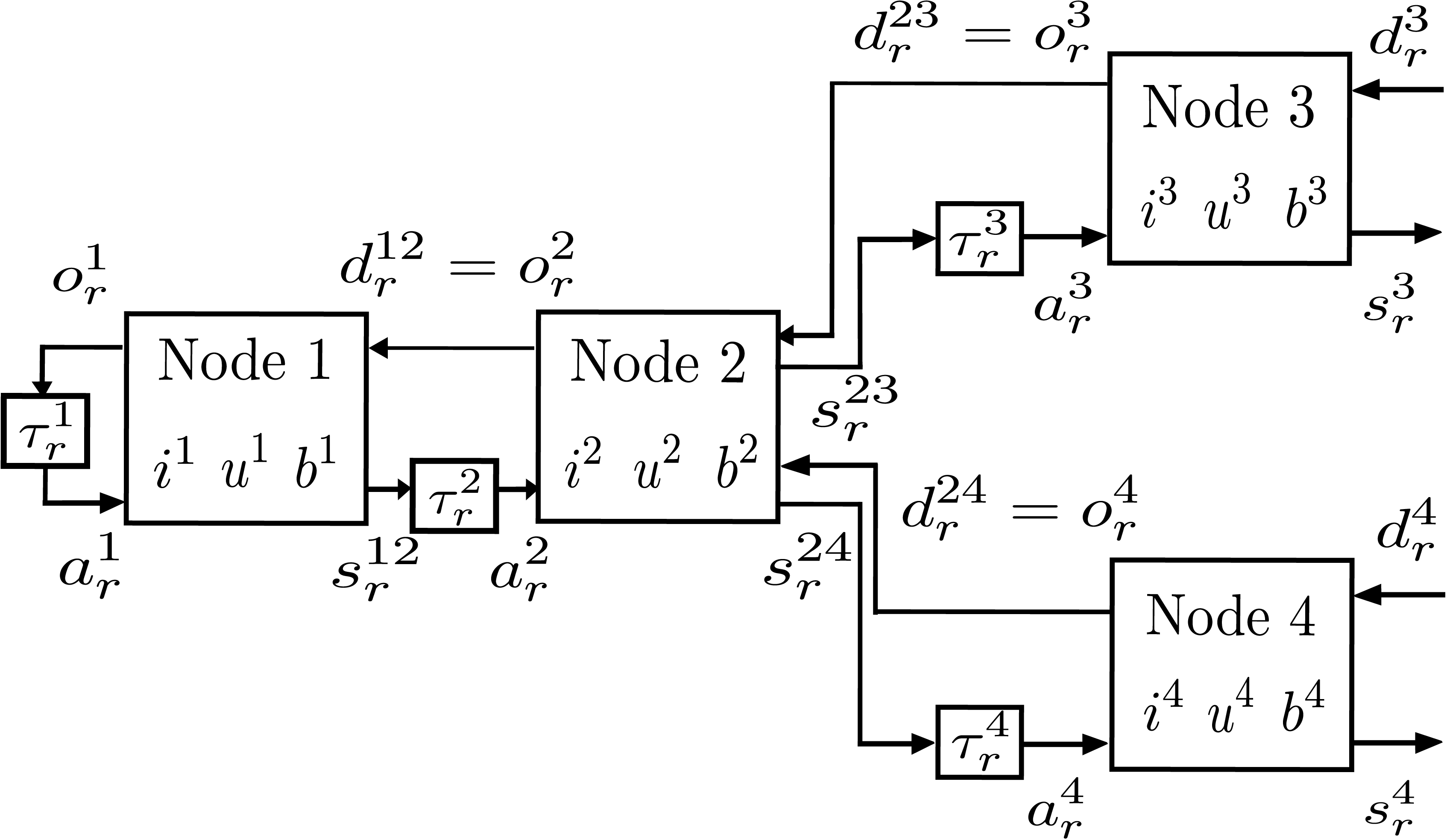
Figure 2: An idealized divergent multi-echelon supply chain network model with four nodes.

Since the multi-period variant of the IM problem was considered, each discrete time period is represented by a time-step in the environment where each episode has a fixed length of $T$ time-steps. At each step, when the agents take their actions, the transition dynamics of the system can be described by the following sequence.

1. All nodes place their replenishment order, $o_{r}^{m}$, to their upstream node except the root node where the replenishment order triggers the production of the good.

2. Nodes receive the goods shipped by their upstream node after a given lead time $\tau_{r}^{m}$. The lead time can be deterministic or stochastic based on the experimental condition used, as described in §2.2. The acquisition is zero for each node $m$ when $t<\tau_{r}^{m}$.

3. All nodes not in $\mathcal{C}$ receive a demand $d^{m_{d}}$ from each of their downstream nodes, (equal to their replenishment order), while nodes in $\mathcal{C}$ receive customer demand.

4. This demand is fulfilled along with any backlog $b^{m_{d}}$ from the available inventory at each node, $i^{m}$ as well as any goods received from an upstream node, $a^{m}_{r}$. Fulfillment priority is given to the existing backlog.

5. Any demand from a downstream node that is unfulfilled is added to the node’s existing backlog. All backlog at the end of the time period incurs a cost. The backlog update is given by

   $$b^{m}[t+1]=b^{m}[t]+\sum_{d\in\mathcal{D}_{m}}d^{m_{d}}[t]-\sum_{d\in\mathcal{D}_{m}}s_{r}^{m_{d}}[t].$$ (2)

6. The inventory at the end of the time period at each node is also updated after sales and acquisition with the following update rule

   $$i^{m}[t+1]=i^{m}[t]+a_{r}^{m}[t]-\sum_{d\in\mathcal{D}_{m}}s_{r}^{m_{d}}[t]$$ (3)

   This is surplus inventory that is held at a cost.

7. Finally, the pipeline inventory/unfulfilled orders $u^{m}$ at the end of the time period is updated using

   $$u^{m}[t+1]=u^{m}[t]+o_{r}^{m}[t]-a_{r}^{m}[t]$$ (4)

It is worth noting that the environment was built using the OpenAI Gym framework (Brockman et al., 2016).

3 Multi-Agent Reinforcement Learning

Reinforcement learning has been shown to learn re-ordering policies for the multi-echelon IM problem that are competitive with methods used in industry Hubbs et al. (2020); Perez et al. (2021). However, learning the optimal policy becomes more difficult for a centralized agent as the problem space becomes larger for larger SCNs. More importantly, SCNs are made up of separate entities with limited information sharing that would make any centralized solution infeasible. Since the multi-echelon IM problem can be naturally decomposed into a multi-agent system where each node is controlled by an agent, MARL can help overcome these constraints.

MARL algorithms can however have varying levels of decentralization. In Claus and Boutilier (1998), the authors classify MARL methods as being either joint action learners (JALs) or independent learners (ILs). JALs can observe the actions of all other agents while ILs can observe only their actions. The limited observability of ILs makes the environment non-stationary from the agent’s perspective, which may lead to sub-optimal policies. While JALs do not have that limitation, they are not practical in most real-world applications due to the agents being physically unable to access the actions and observations of other agents in the environment. However, with access to a centralized simulation environment, agents could be allowed to view the actions and observations of other agents during training only and yet execute actions in a decentralized manner allowing the agents to be deployed separately as with the centralized training decentralized execution (CTDE) framework detailed by Kraemer and Banerjee (2016). Both independent and joint action learners are investigated by leveraging different MARL algorithms with varying levels of information sharing.

3.1 Algorithms

In order to find the distributed optimal re-order policy, multi-agent variations of Proximal Policy Optimization (Schulman et al., 2017) were investigated. PPO has been successfully applied in many control problems in recent years and is simple to tune relative to other RL algorithms. The particular PPO algorithm used in this work utilizes an actor-critic approach and is discussed further in A. Three distinct multi-agent implementations of PPO were investigated in this work, each with varying levels of decentralization.

The first two are variations of Independent Proximal Policy Optimization (IPPO) (de Witt et al., 2020). IPPO simply involves independent agents, each utilizing PPO in order to maximize a shared team reward. Given the use of a shared reward it is important to highlight the difference between the single agent implementation is that each agent acts according to observation of its own local state information and follows its own unique policy gradient in parameter updates. Previous results report that this form of IL matches or outperforms JALs such as QMIX (Rashid et al., 2018) on benchmark maps of the Starcraft multi-agent challenge (Samvelyan et al., 2019). Furthermore, the authors argue that ILs such as IPPO scale better than JALs with the number of agents as they do not face the issue of a growing observation space. The two implementations of IPPO we investigate vary in the degree of information sharing for the formation of each agent’s policy gradient and therefore in the degree of decentralization. In the first implementation, each agent, controlling node $m$, uses and updates its own independent policy $\pi_{\theta_{m}}$ and will be referred to as IPPO in this paper. The second, which will be referred to as IPPO with shared network, is similar to the original implementation where agents share the same network parameters and thus update a single policy $\pi_{\theta}$ and sample actions conditioned on their own observation. The observation is augmented to include a unique identifier for each agent as an additional input. The difference between the two implementations is highlighted in Figure 3.

The third method investigated is a JAL implementation of PPO called Multi-agent Proximal Policy Optimization (MAPPO) first proposed in Yu et al. (2021) and was shown to achieve state-of-the-art performance. In this method, each agent has an independent actor-network that takes as input the agent’s observation only, while utilising a central critic network. The central critic network can be shared amongst all agents, taking as input all agent observations and actions. Another implementation of the centralized critic involves each agent having their own critic network that takes as input the agent’s own observation as well as the observations and actions of all other agents. The latter implementation was used in this work. While centralized training is required to provide the critic with the actions of other agents, each agent can still execute actions in a decentralized manner as the actor network takes only the agent’s own local observations as input. The use of a centralized critic during training makes the environment more stationary from the agent’s perspective as it can observe all other agents’ actions. Training is improved as each agent has access to better estimates of the value function $V(\textbf{s})$. This ultimately provides more stable learning dynamics in the identification of the optimal joint policy.

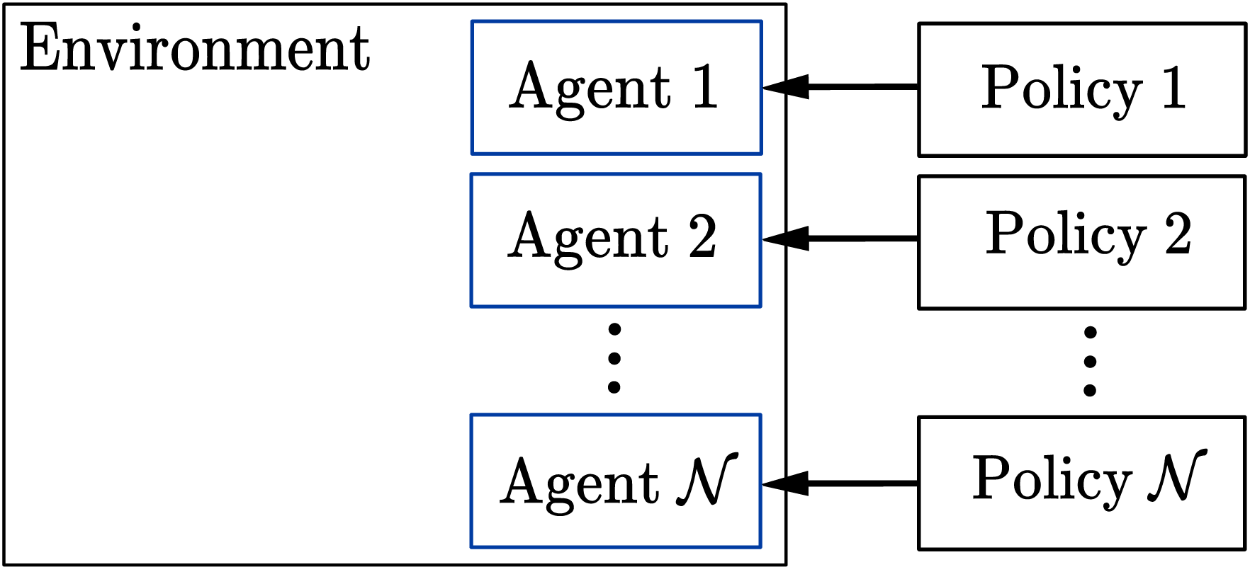
(a) Independent policies.

(b) Shared Policy.

Figure 3: The difference between agents with independent policies and parameter sharing.

3.2 Neural Network Architecture

An actor-critic architecture was utilized where each agent (or set of agents in the case of shared policies) use two neural networks. The critic network is used to estimate the state-action value function $Q(s,a)$, parameterized by parameters $\phi$, while the policy $\pi$ is parameterized by an actor network with parameters $\theta$. The general structure of the networks used in this work is shown in Figure 4.

Two different neural network architectures were investigated to assess whether the use of recurrent neural network (RNN) layers would lead to better re-order policies. This was motivated by time-dependencies in the inventory management problem and partial observability of individual node agents which result in an environment with non-Markovian characteristics. In Wierstra et al. (2007) the authors propose the recurrent policy gradient, which is a policy gradient method that utilizes RNNs, particularly Long Short-term Memory layers (Hochreiter and Schmidhuber, 1997). It was argued that by combining policy gradient methods with back-propagation through time (Werbos, 1990), one can improve the performance of RL agents in partially observable MDPs (POMDPs), where the agent does not have full state observability. In cases where the current state does not capture the history of the system, RNNs would alleviate this issue through the use of their hidden states $h_{t}$, which would capture the history of the system. For example, the presence of lead times $\tau$, means the true rewards associated with a particular action are not immediate, therefore contextualizing on history may help remedy the breakdown in the Markovian problem structure.

The first neural network architecture considered consists of a multi-layer perceptron architecture with two fully connected hidden layers as shown in Figure 4(a) (denoted as FC1 and FC2 in the figure). The second architecture resembles the first with an additional RNN layer as shown in Figure 4(b). In the case of MAPPO, the critic network was modified to take the agent’s own local observation as well as the observations and actions of all other agents that occurred in the same time step. While having a different architecture for the centralized critic and actor networks may be beneficial, this was not explored here.

Agents were trained using both neural network architectures for all the MARL algorithms we investigated in a four-stage serial supply chain to allow for comparison between them. While it was hypothesized that the use of an RNN-based network would significantly improve the performance of the multi-agent system due to each agent’s limited observability, they were found to provide little to no performance improvement for all the MARL algorithms. Furthermore, they resulted in significantly longer training time and a higher deviation of rewards. Therefore the neural network architecture shown in Figure 4(a) was used for the RL algorithms in all the experiments in §4. This analysis is described in further detail in B.

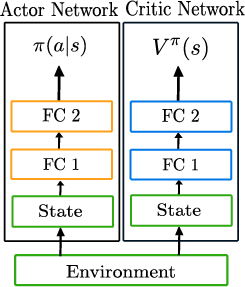
(a) Network without RNN.

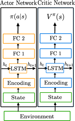
(b) Network with RNN.

Figure 4: The neural network architecture, composed of fully connected (FC) hidden layers, used by the RL agents.

3.3 Formulation

We describe the state and action spaces of the MARL agents for the dec-POMDP described in §2.3. In the multi-agent version of the IM problem considered in this work, each node, $m$, in the SCN is controlled by a separate agent, $j$. Each agent gets an observation, which extends to variables associated with the node it controls only and decides the optimal action, re-order amount, for the node.

Action Space The action each agent takes is the replenishment order at the node controlled by the agent. While the goods are traded in integer quantities as described in §2.3, a continuous action space was used. This was deemed a reasonable assumption given the requirement for the quantities to be integer. However, if the potential space of reorders was discretized more coarsely this assumption may demand revision. The action space of the policy was set to lie in the interval $[-1,\hskip 2.84526pt1]$ as recommended by Raffin et al. (2019). The output actions of the agent were then re-scaled to the physical replenishment order range of $[0,\hskip 2.84526ptO^{m}_{r_{\text{max}}}]$ and rounded to the nearest integer.

Rewards The main objective of the IM problem in this work is to maximize the total profit in the whole SCN which would require agents to collaborate in order to achieve a common goal. Therefore the agents share the overall total reward such that the reward received by each agent at every time-step from the environment is

$$\frac{1}{M}\sum_{m=1}^{M}P^{m}s_{r}^{m}[t]-C^{m}o_{r}^{m}[t]-I^{m}i^{m}[t+1]-B^{m}b^{m}[t+1],$$ (5)

which is simply the mean of the profit earned by each node and therefore agent. Therefore actions taken that hurt overall profit will result in a lower reward for the agent, even if it increases the agent’s node’s profit.

State Space RL algorithms rely on the Markov assumption, which means the information contained within the state is sufficient to decide the action to take. This would lead to the conclusion that the more information captured by the state in each time step, the more this Markovian assumption is satisfied, leading to successful agent learning. However, unnecessary information may make it harder to learn the underlying system dynamics and therefore a good policy. It was therefore investigated which environment variables described in §2.3 should be added to the state vector.

The amount of on-hand inventory $i$, off-hand or pipeline inventory $u$ and backlog $b$ at each stage at the start of the time period were identified as crucial variables (the base state) since they describe the order and material flow throughout the SCN. Other variables identified as potentially important are the demand and actions in the $N$ previous time steps and the incoming shipment from an upstream stage. The incoming shipment variable is essentially a vector of size $\tau_{m}$ where each element represents the amount of goods being shipped and the index represents how many time-steps away it is from arriving at the node. It should be highlighted that if lead time is to be described as a random variable, then in general this part of the state is partially observed and can only be estimated via a forecast. This state vector is illustrated in Figure 5 below where the superscript denotes the time-step of each variable.

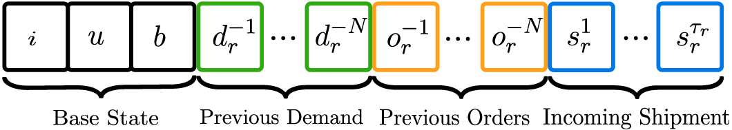
Figure 5: Node state representation configuration used by the RL agent.

For all the MARL algorithms considered, agents were trained with different combinations of the variable groups in Figure 5 in a four-stage serial supply chain. The mean episode rewards of the trained agents were compared to assess which combination of variables in the agents’ observations lead to the best performance for each algorithm. This analysis was done for each algorithm given the varying levels of information sharing between them which may affect what information is useful to include in the agents’ observations. The hyperparameters of the algorithms were tuned for each combination of state variables to ensure a fair comparison between them. This analysis is described in further detail in B.

Following this analysis, it was found that the best performance for both IPPO algorithms was obtained with a state vector containing previous demand and incoming shipments in addition to the base state. While for MAPPO the best performance was achieved with all variable groups. In both cases the optimal of previous time-steps $N$ was found to be 1. These state vectors are used for numerical simulations in §4.

4 Experiments

The performance of the different MARL agents is investigated in different configurations of the IM problem with the aim of assessing which MARL method performs best. We also investigate how our MARL implementations compare against the distributed shrinking horizon LP-based method (DSHLP) described in §F as well as a centralized RL agent.

The centralized single agent has full observability, where the agent’s state consists of the observations of all nodes. The agent’s action is the re-order amount for each of the nodes in the SCN. The agent was trained using the same way as the MARL agents as described in B. The hyperparameters of the centralized RL agent as well as the MARL agents used to obtain the results below, are detailed in D.

All algorithms are compared against the performance of an Oracle, which solves the IM problem as a deterministic problem with all customer demand known a priori using centralized LP.

4.1 Base Case: Four-stage Chain

This was the base case considered during the implementation of the RL methods due to its resemblance to the original beer distribution game (Sterman, 1989) and for which the hyperparameter values of the algorithms used were tuned. The particular configuration used is presented in Table 4. In order to assess the algorithms, we observe the performance of the trained agents on 200 simulated test episodes with 30 time-steps each and customer demand following a Poisson distribution with $\lambda_{\text{Poisson}}=5$. The same test settings were used throughout all simulations described in this section.

The metrics used for comparison were the mean episode reward, inventory and backlog. Inventory and backlog refer to the mean inventory and backlog at the end of each time step in the entire SCN over an entire episode. The main metric of interest is the mean episode reward, however, the other metrics help provide intuition behind the performance achieved by each of the policies and how close their performance is to the optimal performance i.e. the Oracle. The results are presented in Table 2.

Table 2: Average performance metrics of the RL and LP algorithms for test episodes in a four-stage serial supply chain network.

Method	Reward	Oracle	Inventory	Backlog
Oracle	619.4	1.00	49.3	2.7
DSHLP	416.8	0.67	75.8	160.0
Single Agent	477.1	0.77	183.4	84.0
IPPO	443.8	0.71	317.9	64.8
IPPO shared	439.4	0.71	263.2	100.1
MAPPO	463.0	0.75	222.7	81.0

It can be seen that all MARL methods outperform DSHLP in terms of the mean reward achieved. While the MARL algorithms seem to have a larger level of inventory on average than DSHLP, they had a much lower level of backlog on average. Of the MARL algorithms considered, the JAL MAPPO algorithm has achieved the best performance. The JAL MAPPO outperforms both ILs, which have a similar performance. This indicates there is an advantage to ensuring observability during state-value function learning - allowing for better-performing agents that are better able to coordinate. While the centralized RL agent performs better than all the MARL algorithms, its mean reward is marginally better than that achieved by the MAPPO agent, where MAPPO achieves only two percentage points less than the centralized agent. We can observe the average performance of each distributed algorithm across an episode in Figure 6 where we show the average cumulative profit across time steps.

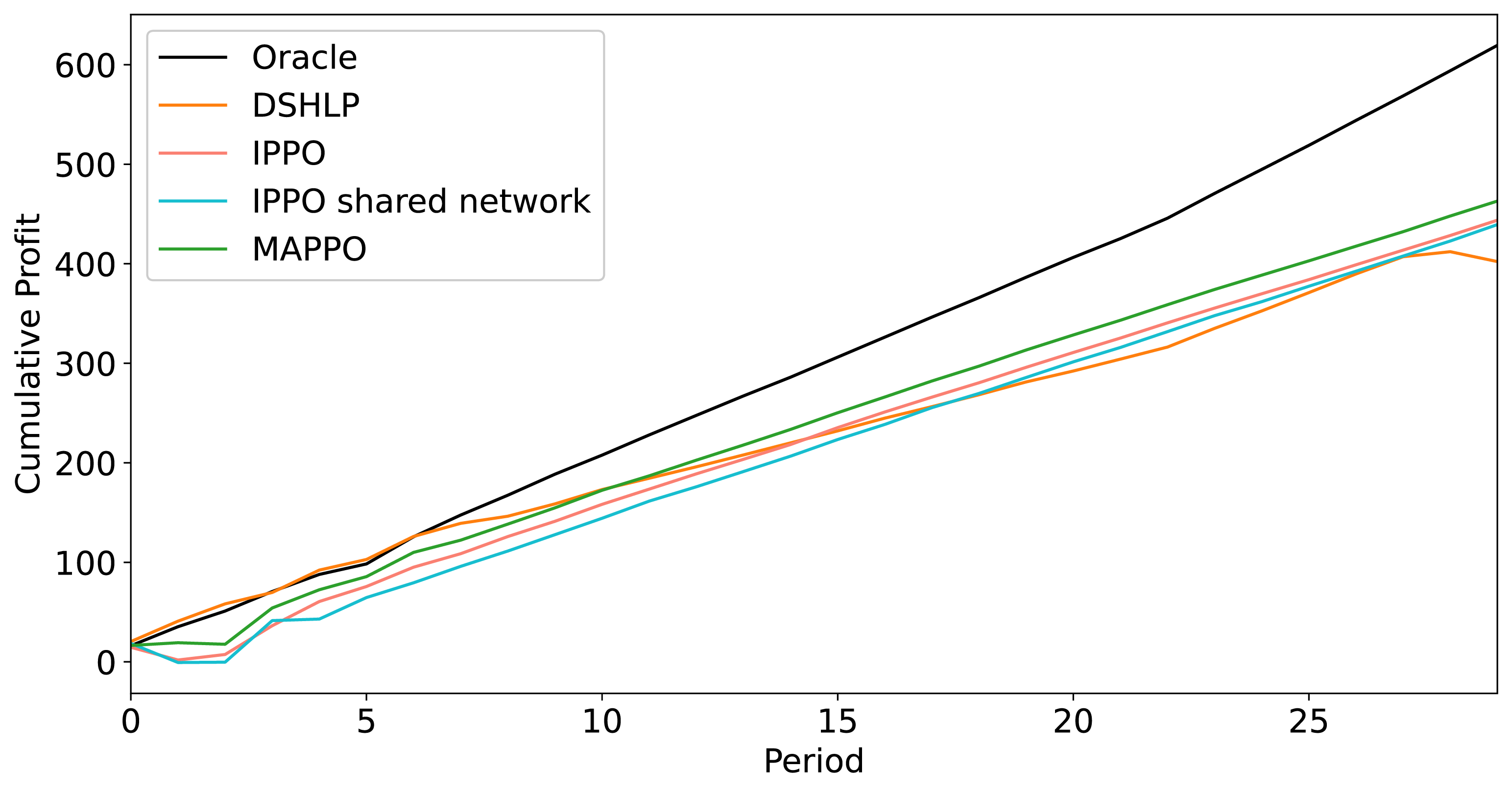
Figure 6: The average cumulative profit achieved by the multi-agent RL algorithms in a four-stage supply chain network compared with LP implementations.

One can see that while DSHLP initially performs better, all MARL algorithms eventually generate more profit with MAPPO consistently outperforming the other two MARL methods. While they generate less absolute profits than the Oracle, as is expected, the profit generated by all MARL agents across episodes follows the same trend as the Oracle.

4.2 Divergent Supply Chain Network

The performance of the MARL methods is investigated for a divergent SCN where the network shown in Figure 2 is considered with the configuration in Table 12. Divergent SCNs require more coordination as there is more than one source of external uncertainty due to the presence of multiple nodes with customer demand and divergent nodes are required to fulfil the demand of multiple nodes simultaneously. The dynamics of the system are also slightly different since nodes have to fulfill backlogs before current demand, which could make lead times more difficult to learn for nodes that share an upstream node. The performance of the different algorithms for the SCN is shown in Table 3.

Table 3: Average performance metrics of the RL and LP algorithms for test episodes in a divergent supply chain network.

Method	Reward	Oracle	Inventory	Backlog
Oracle	926.3	1.00	26.8	4.0
DSHLP	754.3	0.81	160.8	159.1
Single Agent	716.1	0.77	265.2	116.3
IPPO	642.3	0.69	356.2	171.4
IPPO shared	563.3	0.61	542.3	122.4
MAPPO	651.2	0.70	443.5	96.8

The DSHLP algorithm outperforms all MARL algorithms for this divergent SCN with a 10 percentage point difference (in terms of the optimal outcome). DSHLP also outperforms the centralized RL, which we include for reference, showing that data-driven methods might not handle divergent SCNs as well as serial SCNs and might not necessarily outperform traditional model-based optimization methods in all cases. That being said, using a higher network capacity and retuning algorithm hyperparameters (as discussed in Section A) for the divergent SCN might lead to better MARL performance due to the increased complexity of this type of chain. Furthermore, MAPPO and IPPO still learn a decent policy while having an execution speed that is orders higher than DSHLP.

As with the four-stage chain, MAPPO outperforms the other IPPO algorithms, however, its performance is close to IPPO. Unlike previously, using a shared network with IPPO leads to much worse performance. This could be due to the fact that different nodes experience slightly different dynamics in the divergent SCN as opposed to nodes in a serial SCN. For example, the policy of the divergent Node 2 with two downstream nodes, will be different from the other nodes, therefore using a shared network will lead to worse overall performance. Using a shared network therefore might be limited to scenarios where all nodes in a SCN experience the same dynamics.

4.3 Uncertainty

The performance of the different algorithms to disturbances in customer demand and lead time uncertainty were investigated to assess their robustness for the serial four-stage SCN described in §4.1. In the analysis below we show the performance of the different MARL algorithms re-trained at the different levels of uncertainty, as described in §2.2.

Customer Demand While customer demand is uncertain, it still follows a known distribution. This is explicitly modeled in the model-based optimization method but learned by the RL methods from observations of different realizations of demand during training. In order to investigate the robustness of the different algorithms to non-stationary customer demand we use the S2 setting for uncertainty as described in §2.2. The mean reward relative to the Oracle achieved by the different algorithms at 3 different levels of $p_{d}$ is shown in Figure 7(a).

(a) Effect of uncertain customer demand.

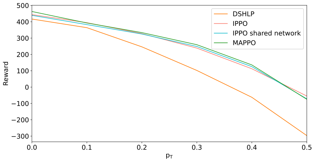
(b) Effect of uncertain lead times.

Figure 7: Effect of uncertainty in system parameters on the performance of the multi-agent RL algorithms.

MARL methods perform better in terms of absolute reward with MAPPO and IPPO both outperforming the distributed LP method. IPPO seems to be the most robust among the MARL methods experiencing the smallest drops in performance, however, MAPPO still outperforms IPPO in absolute terms across all levels of $p_{d}$ tested and experiences marginally larger drops in performance. Using a shared network with IPPO however, leads to a large drop in performance which shows that sharing experience across agents using the same network is less robust.

While it was expected the model-free methods would be more robust to spikes in customer demand due to not explicitly assuming the distribution it is drawn from as well as being trained on this noisy demand, they seem less robust to that disturbance than the traditional distributed LP method. It can be seen that the distributed LP method experiences smaller drops in performance relative to the base case than the MARL methods, which might indicate that it is more robust to that type of uncertainty.

Lead Times Fixed lead times are explicitly modeled in the LP method as a constraint in the optimization problem of the system as in (LABEL:eqn:_acquisition), but it is only learned from episodes of experience by the RL agents. We investigate the robustness of the different distributed algorithms to stochastic delivery lead times using the uncertainty setting S3 as described in §2.2. The mean reward achieved by the different algorithms is shown in Figure 7(b).

It can be seen that the performance of the MARL is less affected by the stochastic delivery lead times relative to the distributed LP method. They outperform the distributed LP method significantly at levels of $p_{\tau}$ as the model-based method experiences a severe drop in performance. This large performance difference could be attributed to the fact that the model-based LP method explicitly models deterministic lead times and therefore experiences this large drop in performance. Another reason for MARL methods’ outperformance could be their higher inventory levels as seen in Tables 2 and 3 which makes them more robust to lead time uncertainty. This is in contrast to the stochastic customer demand where the distribution is taken into account, thus it is more robust to customer demand uncertainty. All MARL methods seem to have very similar performance all experiencing roughly the same drop in performance. MAPPO seems to experience the largest drop in performance while IPPO experiences to smallest, however, the difference is negligible.

4.4 Supply Chain Network Size

The effect of the size of the SCN on the performance of the different RL algorithms presented is investigated. The performance of the algorithms was assessed in three serial SCNs with a different number of stages (two, four and eight with configurations for two and eight-stage SCNs in Tables 13 and 14 respectively). The agents of each algorithm were trained in the new environments, however using the same hyperparameter values optimized for the four-stage SCN in §4.1. The mean and standard deviations of rewards achieved by each algorithm over 200 test episodes normalized by the Oracle’s mean reward are shown below in Figure 8 for the different SCNs.

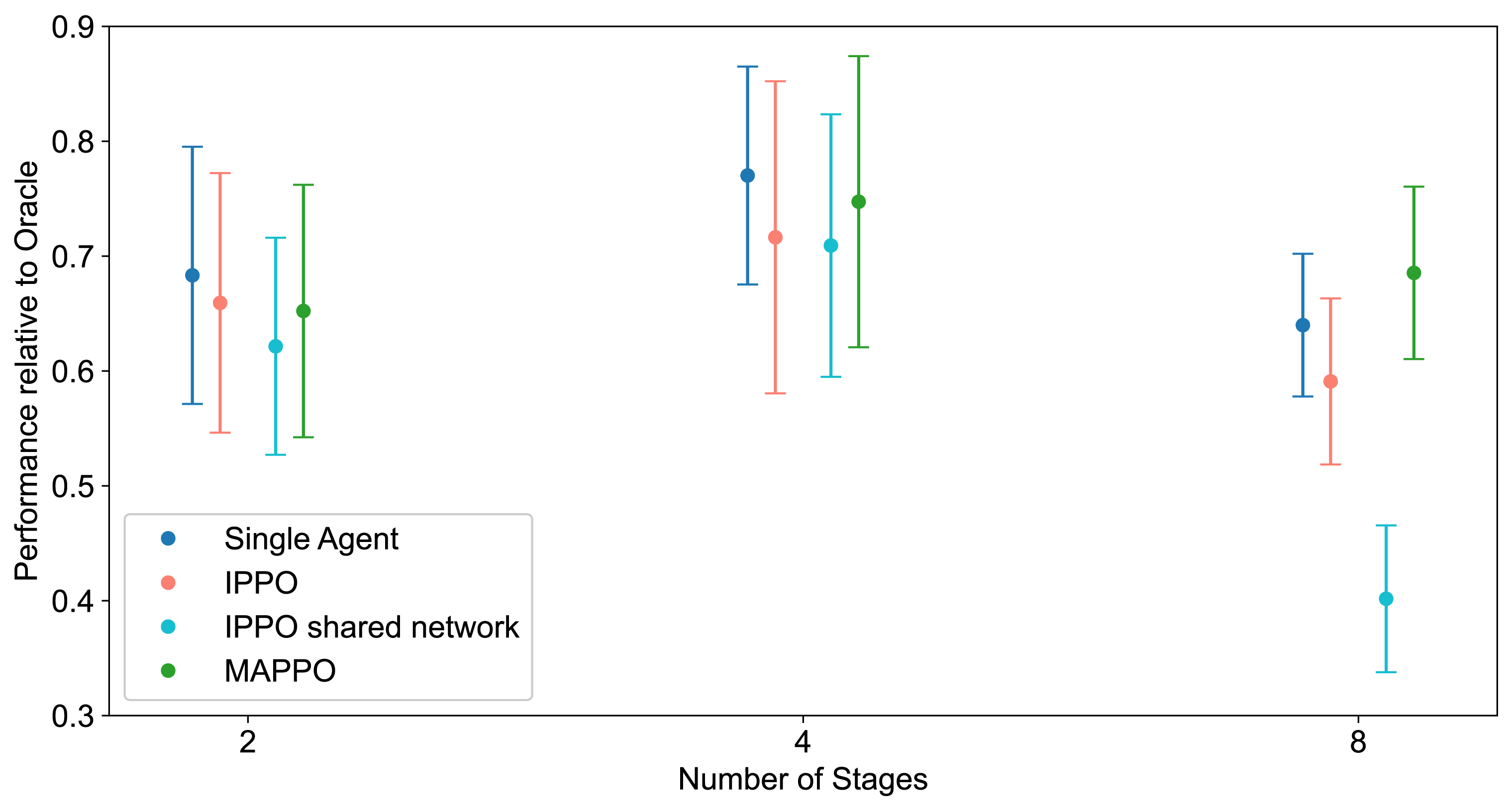
Figure 8: Effect of supply chain network size on the performance of the multi-agent RL algorithms, relative to a perfect information centralized LP implementation.

The MARL methods seem to be more robust to changes in the size of the problem. While the single agent outperforms the MARL methods in most cases when measuring absolute performance, its performance relative to the base four-stage case is worse than the MARL algorithms (with the exception of IPPO with a shared network). This can be seen by observing the change in performance from the base case. MAPPO even outperforms the single agent in the eight-stage SCN, while IPPO performs similarly to the single agent. A likely reason for this is that as the dimensionality of the SCN increases, the optimal policy function may no longer lie in the space of functions that can be expressed by the policy function structure of the single agent, suggesting a benefit to exploiting the problem structure through decentralization. The performance of IPPO with a shared network also suffers for the larger eight-stage SCN for possibly the same reason, as the shared network may not have sufficient capacity for providing a good policy for a larger number of agents.

It should be noted that if re-optimization of the single agent’s hyperparameters had been considered the single agent policy may have not been subject to such a result with increasing supply chain size. The single agent is more affected by the problem’s size than the MARL algorithms as both the state and action spaces of the problem grow, therefore may benefit from a different policy function approximation or different hyperparameter values. However, for agents in MARL algorithms, the size of the SCN does not affect a node’s individual sub-problem therefore the action and state spaces stay constant. Because of this, MARL algorithms are more robust to changes in the problem’s size, regardless of hyperparameter values. This is a desirable attribute as the structure of SCNs can change over time and this result indicates a high-performance MARL algorithm can be transferred across different problems.

4.5 Training without Noise

In this section, we investigate how uncertainty in the form of customer demand and lead time disturbances, as described above in §4.3, affect the performance of the MARL methods. Previously, we investigated the performance of MARL methods when trained and evaluated on different uncertainty settings, S2 and S3, and compared the results to the base-case four-stage serial SCN with S1. In this section, we train the MARL methods on the base case uncertainty settings S1, but then evaluate the policies under the uncertainty settings S2 and S3. We compare their results to the centralized RL agent to assess the robustness of the distributed data-driven methods. This is shown in Figure 9(a) for S2 we plot the mean reward of the different algorithms at the different levels of disturbance, where the solid lines represent the algorithms trained on data with S2 while the dotted lines represent the algorithms trained with S1.

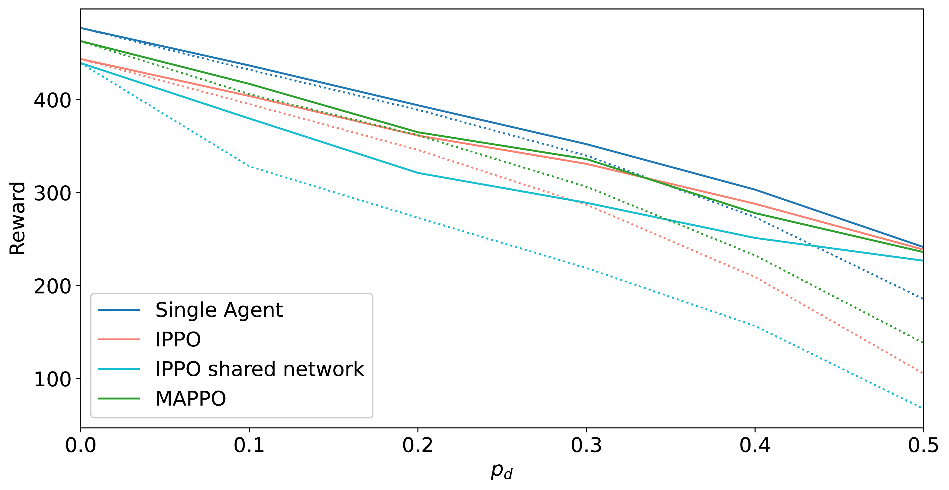
(a) Customer demand disturbance.

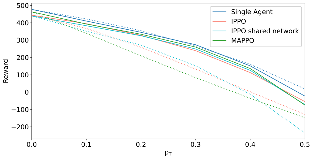
(b) Lead-time disturbance.

Figure 9: The performance difference of the multi-agent RL algorithms when training with S2 against training with S1 (dotted lines).

We can see that the performance of all algorithms improves significantly when they are trained on data with non-stationary customer demand as opposed to when they are not, with this improvement being more significant at higher levels of $p_{d}$. When the algorithms are not trained on non-stationary customer demand, we can see that MARL methods are less robust to disturbances in customer demand than the centralized single agent, experiencing larger drops in performance. This could be due to the nature of the disturbance, which appears at the customer-facing node, paired with the limited observability of agents during execution. The centralized agent can observe the whole SCN, however for the MARL agents without communication, information flows between nodes at the speed of order flows, thus nodes further upstream cannot account for the disturbance before it is too late. While using MAPPO or IPPO leads to a marginally larger drop in performance than the single agent, both algorithms perform worse in absolute terms. However, MARL algorithms experience a much larger performance gain than the single agent when trained on data with non-stationary customer demand and approach the performance of the single agent in absolute terms at higher noise levels.

The same behavior can be observed when using stochastic delivery lead times as shown in Figure 9(b). In this case, the effect is even more significant with MARL algorithms performing significantly worse when trained with deterministic lead times with the S1 uncertainty setting. This is due to the fact that the state configurations used for MARL algorithms include incoming shipment information which becomes a forecast under lead-time uncertainty. However, training on data with stochastic delivery lead times in S3 results in the MARL agents almost matching the performance of the centralized agent across a range of noise levels. This shows the robustness of MARL algorithms in terms of training (while utilizing the same algorithm configuration) which is particularly useful for applications such as SCNs where structural changes to the data-generating process happen over time and algorithms need to be re-trained.

4.6 Independent Rewards

In all the above simulations and analyses, MARL agents were set to maximize the total SCN profit as each agent receives the average total profit as a reward. Using shared rewards leads to more stable training as well as more coordination (especially in the absence of communication) as agents learn a policy aimed at maximizing the total SCN profit which would be desired as a real-life objective. However, in most real SCNs nodes will seek to maximize their own individual reward as each node is an independent entity with its own objectives. It was found, however, that training MARL agents with independent rewards lead to unstable training as well as significantly worse performance. We compare the performance (in terms of total SCN profit achieved) of the different MARL algorithms trained with shared rewards against those trained with independent rewards on 200 episodes to assess the effect of using independent rewards. This is shown in Figures 10(a) and 10(b) for the four-stage and divergent SCNs respectively where dotted lines represent the algorithms trained with independent rewards.

(a) Serial SCN.

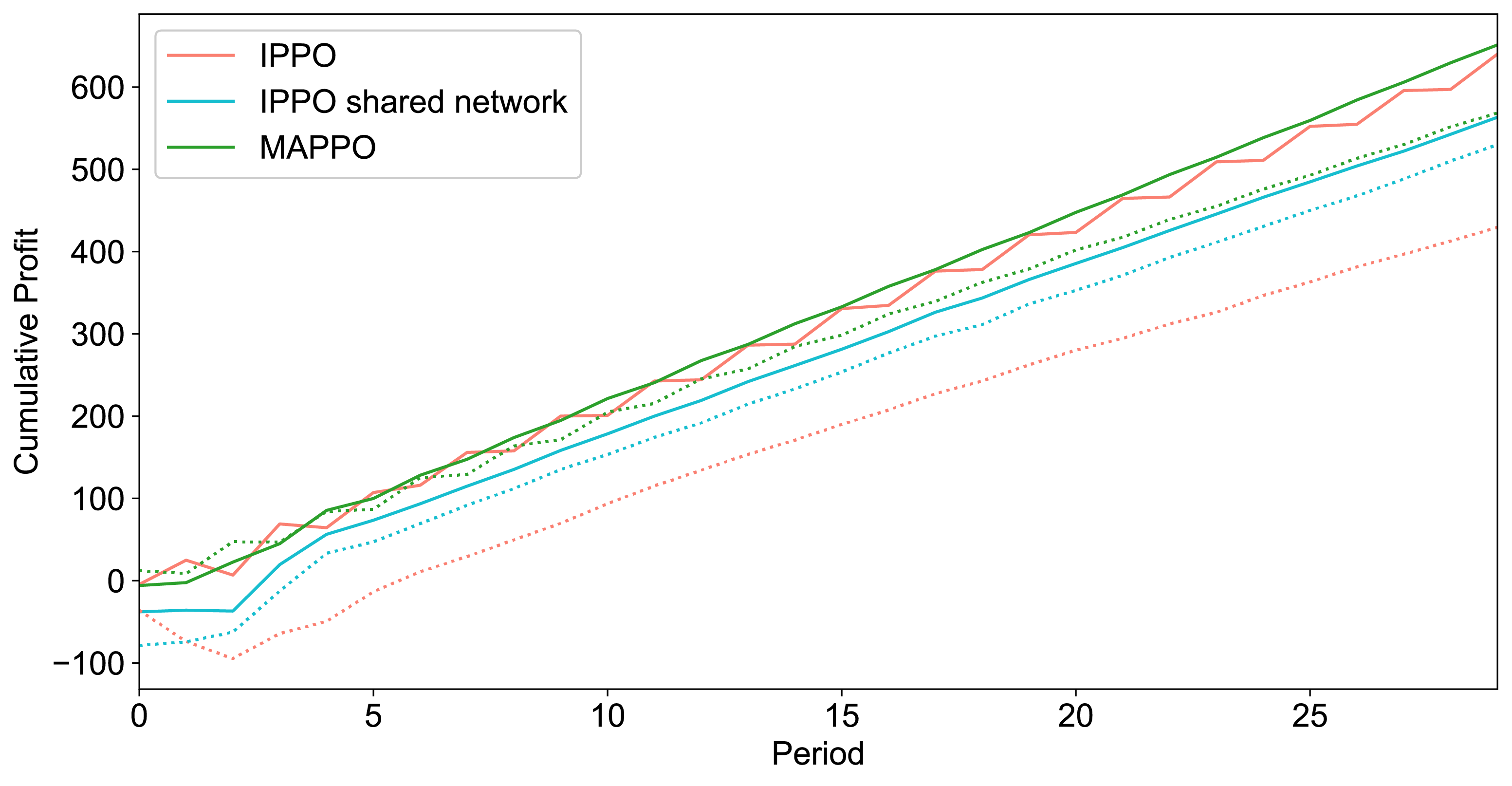
(b) Divergent SCN.

Figure 10: The effect of using independent rewards (dotted lines) on the multi-agent RL algorithms compared with the use of shared rewards (solid lines).

It can be seen that in both cases, using IPPO with a shared network resulted in the smallest drop in performance where the agents were still able to learn a good policy. IPPO on the other hand experienced the largest drop in performance in both cases. Using a shared network might result in more coordination as the same network is used to find a reward maximizing policy for all agents even when utilizing independent rewards, whereas IPPO with independent rewards is completely decentralized. MAPPO also experiences a large drop in performance, especially in the four-stage serial SCN, even while not being completely decentralized due to the use of global observation for the critic network. That being said, the MAPPO algorithm was still able to learn a decent policy for the divergent SCN with independent rewards.

4.7 Summary

Three different MARL methods were analyzed in different SCN configurations to assess their effectiveness for the IM problem. During online execution, MARL methods are orders of magnitude faster online as compared with traditional model-based LPs. While this faster execution comes at the cost of offline training, it also provides complete decentralization with no requirement to coordinate computation online. The computational efficiency of trained agents also becomes more important as the size of SCNs, and hence the IM problem, becomes larger and more complex. In terms of performance, all the MARL methods considered outperform a corresponding distributed LP method to the problem in serial SCNs as seen in §4.1. While this improvement in performance did not extend to divergent SCNs as seen in §4.2, IPPO and MAPPO still learn a good policy while having the added advantage of being orders faster during online execution than DSHLP. In terms of robustness to external uncertainty in §4.3, we find that due to their data-driven model-free nature, the MARL methods were much more robust to lead time uncertainty than DSHLP and manage to outperform it over a range of customer demand disturbance levels. Of the MARL methods tested, MAPPO and IPPO were found to have consistently good performance, almost matching that of an equivalent centralized implementation. Using IPPO with a shared network, however, leads to performance drops for larger SCNs such as the eight-stage serial SCN, or SCNs where all nodes don’t share similar dynamics like the divergent SCN in §4.2. When using independent rewards as in §4.6 it was found that using IPPO with a shared network still leads to a good policy in terms of total SCN profit with a significantly smaller drop in performance than MAPPO and IPPO.

5 Conclusions

Three distributed data-driven methods utilizing MARL were proposed (IPPO, IPPO with shared network and MAPPO) to find a dynamic re-order policy for IM problem. This offers a more practical solution to real-world supply-chain networks as they are made up of independent entities. While it was hypothesized that the use of RNNs would improve the performance of MARL agents given their partial observability, it was found that using RNNs did not lead to better policies. The MARL methods were assessed across different SCN configurations and the results have shown that they achieve a performance close to that of the single RL agent centralized solution in terms of total profit achieved. Furthermore, they are more scalable as the solution space of the agents in MAPPO and IPPO does not grow with the size of the problem, with MAPPO outperforming the centralized RL for an eight-stage serial SCN. They also outperform the distributed solution utilizing LP for most cases tested and are more robust to demand and lead-time uncertainty while being orders more computationally efficient during execution. We show that having full observation during training leads to better performance where MAPPO achieved the highest mean rewards across the different SCN configurations tested. IPPO performs similarly to MAPPO but we find that sharing a policy between agents leads to worse performance in the case with IPPO with a shared network.

The results of the proposed MARL solution to the IM problem show decentralized data-driven control provides a good control solution to large-scale stochastic systems. They perform nearly as well as their centralized counterpart while making fewer assumptions and respecting real-world information-sharing constraints. This makes them far more practical and applicable to real SCNs. Furthermore, this shows that MARL is a viable solution for many other similar problems in OR.

In order for the MARL method to handle the more complex systems some improvements would need to be made. The agents’ handling of system disruptions could be improved through the use of differentiable communication channels (Sukhbaatar et al., 2016) which will allow agents to learn to communicate useful information. This would reduce the problem caused by the partial observability of agents as information can be propagated through the system faster than the flow of orders and materials. The use of Graph Neural Networks (GNN) in particular could make use of the underlying SCN graph structure to allow for more efficient and effective communication. GNNs have been shown to improve performance for collaborative agents (Jiang et al., 2020; Meneghetti and Bianchi, 2020) as it allows for better coordination. Furthermore, the use of vertical federated RL Qi et al. (2021) could help overcome the problem of centralization of information during training.

Appendix A Algorithm Description

In this section, we describe the PPO algorithm utilized in this work. Like regular policy gradient methods, the aim is to find a policy $\pi(a|s)$ parameterized by a neural network with parameters $\theta$ that maximizes total episode returns. A surrogate objective $L$ is maximized such that the policy update is given by

$$\theta_{k+1}=\arg\max_{\theta}\mathbb{E}_{s,a\sim\pi_{\theta_{k}}}[L(s,a,\theta_{k},\theta)],$$ (6)

The aim of PPO is to avoid taking steps in parameter space $\theta$ that may cause the policy $\pi_{\theta}(a|s)$ to collapse by ensuring that the new policy does not deviate too much from the old policy.

Therefore, the PPO-clip algorithm utilizes the following surrogate objective.

where $A^{\pi_{\theta_{k}}}$ is the advantage function under policy $\pi_{\theta_{k}}$ which describes the advantage of taking action $a$ in state $s$ according to $\pi(\cdot|s)$ over the policy’s average action in that state. The PPO-clip surrogate objective forces the ratio between the old and new policy to stay with an interval $[1-\epsilon,\hskip 2.84526pt1+\epsilon]$, where the policy clip parameter $\epsilon$ is a hyperparameter, through the use of the clip function.

In addition to the PPO-clip objective, an adaptive KL penalty coefficient was used which adds a penalty on the KL divergence, $d_{KL}$ between the old and new policies and adapts the penalty coefficient until a target KL divergence, $d_{\text{targ}}$ is achieved. The adaptive KL penalty objective is given by (Schulman et al., 2017) as

$$L^{\text{KL}}(s,a,\theta_{k},\theta)=\frac{\pi_{\theta}(a|s)}{\pi_{\theta_{k}}(a|s)}A^{\pi_{\theta_{k}}}-\beta\text{KL}[\pi_{\theta_{k}}(\cdot|s),\pi_{\theta}(\cdot|s)],$$ (8)

where $\beta$ is the adaptive KL divergence coefficient. At each policy improvement step, the KL divergence between the old and new policies is calculated. If $d_{KL}<\frac{2}{3}d_{\text{targ}}$ then $\beta\leftarrow\frac{\beta}{2}$ and if $d_{KL}>\frac{3}{2}d_{\text{targ}}$ then $\beta\leftarrow\beta\times 2$. Therefore, the surrogate objective utilized in the PPO implementation for this work is given by

$$L(s,a,\theta_{k},\theta)=L^{\text{clip}}-\beta\text{KL}[\pi_{\theta_{k}}(\cdot|s),\pi_{\theta}(\cdot|s)]$$ (9)

A good estimate of $A^{\pi}$ reduces the variance of the policy gradient and thus results in fewer samples being required. In this work, the generalized advantage estimator (GAE) (Schulman et al., 2018) was used to estimate the advantage function which is given by

$$A^{\pi}_{\text{GAE}}(s_{t},a_{t})=\sum^{\infty}_{l=0}(\gamma\lambda)^{l}\delta_{t+l}$$ (10)

where

$$\delta_{t}=r_{t}+\gamma V^{\pi}(s_{t+1})-V^{\pi}(s_{t})$$

is the TD-error or advantage function for time-step $t$ with 1-step forward returns, $\gamma$ is the discount factor and $\lambda$ is a hyperparameter that controls the bias-variance trade-off of the GAE estimate. Equation (10) is, in essence, a weighted average of several advantage estimators with different biases and variances. The 1-step advantage estimate $\delta_{t}$ is high-bias and low-variance while higher $l$-step advantages have lower bias but higher variance. Contributions from $l$-step advantages decay exponentially where the decay rate is controlled by $\lambda$. A higher value of $\lambda$, therefore, results in higher variance and lower bias and vice-versa.

The GAE requires values for the value function $V$ which is estimated using a separate neural network with parameters $\phi$. This leads to an actor-critic structure where the actor-network $\pi$ updates the policy $\pi_{\theta}$ using the objective function (9) while the critic estimates the value function of the system’s states $V_{\phi}$ in order to provide more accurate advantage estimates for policy optimization. The algorithm used in this work is summarised below.

Algorithm 1 PPO clip with adaptive KL penalty (Achiam, 2018)

.

1:Input: Initial policy parameters $\theta_{0}$ and initial value function parameters $\phi_{0}$

2:for $k=0,1,2,\dots$ do

3:     Collect set of trajectories $\mathcal{D}$ = $\{s_{i},a_{i},r_{i},s^{\prime}_{i}\}$ by running policy $\pi_{\theta_{k}}$ in the environment.

4:     Compute rewards-to-go $R_{t}$.

5:     Compute GAE advantage estimates $\hat{A}_{t}$ using the current value function estimates $V_{\phi_{k}}$ over several mini-batches using stochastic gradient ascent with Adam. (Kingma and Ba, 2017).

6:     Fit value function using mean-square error

$$\phi_{k+1}=\arg\min_{\phi}\frac{1}{|\mathcal{D}_{k}|T}\sum_{\tau\in\mathcal{D}_{k}}\sum_{t=0}^{T}\big{(}V_{\phi}(s_{t})-R_{t}\big{)}^{2}$$

     over several mini-batches using stochastic gradient descent with Adam.

7:     Update the policy by maximizing the surrogate objective:

$$\theta_{k+1}=\arg\max_{\theta}\frac{1}{|\mathcal{D}_{k}|T}\sum_{\tau\in\mathcal{D}_{k}}\sum_{t=0}^{T}\big{(}L^{\text{clip}}-\beta\text{KL}[\pi_{\theta_{k}}(\cdot|s),\pi_{\theta}(\cdot|s)]\big{)}$$

8:end for

Appendix B Agent Training

In order to determine which variables to include in the state vector or which neural network architecture from Figure 4 we train RL agents for each of the MARL algorithms being investigated on different combinations and compare their performance. To allow for a fair comparison, we tune the hyperparameters of the algorithms for each combination and test their performance for one SCN environment. The hyperparameter tuning is described in more detail in C and the final values used for the algorithms are shown in D.

A four-stage serial SCN was chosen as the base environment over which to tune the hyperparameters with the environment parameters shown below in Table 4 with an episode containing a number of periods $T=30$. Customer demand was assumed to follow a Poisson distribution with $\lambda_{\text{Poisson}}=5$.

Table 4: IM environment configuration for a four-stage supply chain.

Parameter	Symbol	Node 1	Node 2	Node 3	Node 4
Initial inventory	$i[0]$	10	10	10	10
Sell price	$P$	2	3	4	5
Replenishment cost	$C$	1	2	3	4
Storage cost	$I$	0.35	0.30	0.40	0.20
Backlog cost	$B$	0.50	0.70	0.60	0.90
Storage capacity	$I_{\max}$	30	30	30	30
Order limit	$O_{r_{\max}}$	30	30	30	30
Lead time	$\tau$	1	2	3	1

In order to decide on which variables to include in the state vector, different combinations of the state vector groups shown in Figure 5 were tested. The different state vector configurations tested are:

1. Base State

2. Base State + Delayed Shipment

3. Base State + Previous Demand + Previous Orders

4. Base State + Previous Demand

5. Base State + Previous Demand + Previous Orders + Delayed Shipment

6. Base State + Previous Demand + Delayed Shipment

After training each agent state vector configuration from the above with both neural network architectures, to completion, each trained set of agents was tested on the same 1000 test episodes each consisting of a realization of the customer demand over 30 time steps. The mean episode reward for each configuration, along with its standard deviation is shown below for IPPO in Table 5 and for MAPPO in Table 6.

Table 5: IPPO performance of each state-vector configuration/network architecture combination.

State Configuration	1	2	3	4	5	6
Without RNN	410.6 (68.7)	439.9 (81.1)	409.6 (62.7)	419.5 (61.7)	442.9 (65.5)	450.3 (66.6)
With RNN	422.2 (74.3)	413.6 (81.2)	414.8 (84.3)	429.1 (70.5)	434.6 (78.9)	397.1 (93.4)

Table 6: MAPPO performance of each state-vector configuration/network architecture combination.

State Configuration	1	2	3	4	5	6
Without RNN	398.7 (62.6)	407.0 (81.0)	423.8 (61.4)	400.3 (61.1)	436.7 (60.5)	430.3 (72.4)
With RNN	440.0 (89.8)	414.7 (91.3)	400.4 (88.5)	424.0 (73.5)	396.5 (76.5)	425.0 (75.9)

While it was hypothesised that the use of an RNN based network would significantly improve the performance of the multi-agent system due to each agent’s limited observability, the best performing combination for the IPPO (underlined in Table 5 above) did not utilise an RNN. It can also be seen that state vector configurations that included more information through the use of more variables seemed to perform better without the use of an RNN. One explanation could be that knowledge of variables such as previous demand and actions is sufficient to capture enough of the system’s history such that actions can be conditioned on just the observation without the need for the RNN’s internal hidden state.

For MAPPO, the best performing state vector configuration and network architecture combination was actually configuration 1 with the use of an RNN. However, it was only marginally better than using state vector configuration 5 without an RNN. It also had a significantly higher standard deviation of rewards which lead to using state vector configuration 5 without an RNN instead.

The same analysis and training were done for a centralized RL agent controlling the entire SCN, utilizing the same PPO algorithm described in A. The results are shown in Table 7 below. It can be seen that state vector configuration 3 with a neural network not utilizing an RNN achieved the best episode mean reward. This setting is used by the centralized single RL agent in all the results shown in this work.

Table 7: Single-agent performance of each state-vector configuration/network architecture combination.

Network Architecture	1	2	3	4	5	6
Without RNN	465.1 (60.4)	476.3 (53.9)	478.2 (47.7)	437.6 (34.7)	453.6 (43.1)	465.8 (35.4)
With RNN	438.2 (58.5)	453.1 (57.8)	434.6 (73.2)	453.6 (59.7)	455.6 (55.9)	446.0 (58.4)

Appendix C Hyperparameter Optimization

The hyperparameters tuned include PPO-specific hyperparameters such as the number of experiences/time-step collected in every iteration i.e. the batch size $|\mathcal{D}|$ and subsequently the number of epochs and minibatch size for the SGD as well the learning rate for the Adam optimizer. Other hyperparameters include variables relating to the network architecture, particularly the number of neurons in each hidden layer. This is summarised below along with the range of values considered for each hyperparameter in Table 8. For a network without an RNN, the hyperparameter search setting is identical to the one shown below but without the RNN-related hyperparameters (Actor/Critic Encoding layer size and LSTM state size). It is worth noting that ranges in parenthesis refer to search space over a uniform or uniform integer distribution with the parameters of the distribution in the parentheses, whereas ranges in square brackets involve searching among the distinct values within the brackets.

To find the best hyperparameters, the Ray tune library Liaw et al. (2018) was used. Within the Ray tune framework, a population-based training (PBT) Jaderberg et al. (2017) scheduler was used to optimize the hyperparameter values. PBT involves training many neural networks or, in this case, agents, in parallel starting off with random hyperparameter values from prescribed ranges. It then goes for different phases of exploration or exploitation of hyperparameters. In exploration, a new value for a hyperparameter is sampled from the given distribution, whereas during exploitation the parameters of a better-performing agent might be copied.

In this work, 6 agents were trained in parallel. Hyperparameters were perturbed every 4 training iterations with workers training each agent deciding on whether to explore or exploit. This process was stopped after 200 training iterations as preliminary experiments had shown this is sufficient for policy convergence.

Table 8: Multi-agent centralized critic hyperparameter optimization settings.

Hyperparameter	Value range
Batch size, $|\mathcal{D}|$	(1500, 9000)
Minibatch size	(64, 256)
Epochs	(3, 30)
Clip parameter, $\epsilon$	(0.1, 0.4)
Discount factor, $\gamma$	(0.95, 0.99)
GAE parameter, $\lambda$	(0.90, 1.0)
Initial KL coefficient, $\beta$	(0.1, 0.6)
KL target, $d_{\text{targ}}$	(0.003, 0.03)
Learning rate, $\alpha$	[5e-4, 1e-4 5e-5, 1e-5, 5e-6]
FC1 size	[64, 128, 256]
FC2 size	[64, 128, 256]
Actor Encoding size	[16, 32, 64, 128, 256]
Critic Encoding size	[16, 32, 64, 128, 256]
LSTM state size	[64, 128, 256]
Previous length, $N$	[1, 2, 3]

Appendix D Hyperparameter Values

The hyperparameter values for each of the RL algorithms used are shown below in Tables 11, 10 and 9. It is worth noting that the IPPO hyperparameter values were used for both the IPPO and IPPO with shared network algorithms.

Table 9: IPPO hyperparameter values.

Hyperparameter	Value range
Batch size, $|\mathcal{D}|$	3000
Minibatch size	180
Epochs	14
Clip parameter, $\epsilon$	0.21
Discount factor, $\gamma$	0.99
GAE parameter, $\lambda$	0.95
Initial KL coefficient, $\beta$	0.19
KL target, $d_{\text{targ}}$	0.006
Learning rate, $\alpha$	$1\times 10^{-5}$
FC1 size	128
FC2 size	128

Table 10: MAPPO hyperparameter values.

Hyperparameter	Value range
Batch size, $|\mathcal{D}|$	4147
Minibatch size	92
Epochs	12
Clip parameter, $\epsilon$	0.41
Discount factor, $\gamma$	0.966
GAE parameter, $\lambda$	0.973
Initial KL coefficient, $\beta$	0.69
KL target, $d_{\text{targ}}$	0.003
Learning rate, $\alpha$	$1\times 10^{-5}$
FC1 size	256
FC2 size	256

Table 11: Centralized single RL agent hyperparameter values.

Hyperparameter	Value range
Batch size, $|\mathcal{D}|$	3000
Minibatch size	225
Epochs	10
Clip parameter, $\epsilon$	0.22
Discount factor, $\gamma$	0.99
GAE parameter, $\lambda$	0.95
Initial KL coefficient, $\beta$	0.37
KL target, $d_{\text{targ}}$	0.0043
Learning rate, $\alpha$	$1\times 10^{-5}$
FC1 size	64
FC2 size	256
Previous length, $N$	1

Appendix E Supply Chain Network Environment Configurations

The tables below summarise the environment parameters for the different SCN configurations used.

Table 12: The IM environment configuration of the divergent supply chain.

Parameter	Symbol	Node 1	Node 2	Node 3	Node 4
Initial inventory	$i[0]$	10	10	10	10
Sell price	$P$	2	3	4	4
Replenishment cost	$C$	1	2	3	3
Storage cost	$I$	0.35	0.30	0.40	0.40
Backlog cost	$B$	0.50	0.70	0.60	0.60
Storage capacity	$I_{\max}$	30	30	30	30
Order limit	$O_{r_{\max}}$	30	30	30	30
Lead time	$\tau$	1	2	1	1

Table 13: IM environment configuration for a two-stage supply chain.

Symbol	Stage 1	Stage 2
$i[0]$	10	10
$P$	3	2
$C$	2	1
$I$	0.50	0.20
$B$	0.60	0.90
$I_{\max}$	30	30
$O_{r_{\max}}$	30	30
$\tau$	3	1

Table 14: IM environment configuration for an eight-stage supply chain.

Symbol	Stage 1	Stage 2	Stage 3	Stage 4	Stage 5	Stage 6	Stage 7	Stage 8
$i[0]$	10	10	10	10	10	10	10	10
$P$	9	8	7	6	5	4	3	2
$C$	8	7	6	5	4	3	2	1
$I$	0.35	0.30	0.40	0.20	0.35	0.30	0.40	0.20
$B$	0.50	0.70	0.60	0.90	0.50	0.70	0.60	0.90
$I_{\max}$	30	30	30	30	30	30	30	30
$O_{r_{\max}}$	30	30	30	30	30	30	30	30
$\tau$	1	2	3	1	4	2	3	1

Appendix F Mathematical Programming Benchmarks

Linear Programming (LP) was used to find solutions for the IM problem to compare the performance of traditional model-based re-order policies against that of the data-driven model-free RL methods developed. Dynamic re-order policies involve finding the optimal replenishment order level at every time step by solving the optimization problem above. In this work, the multi-period IM problem was solved using a shrinking horizon where at every time-step $j$, the objective to be maximized is

$$\max\sum_{t=j}^{T}\sum_{m=1}^{M}P^{m}s_{r}^{m}[t]-C^{m}o_{r}^{m}[t]-I^{m}i^{m}[t]-B^{m}b^{m}[t].$$ (11)

The only difference to the original optimization problem is that the demand for customer-facing nodes is now equal to the expectation of customer demand $\forall t>j$ for future time steps. The first replenishment order for each node $o_{r}^{m}[j]$ from the solution to the above optimization problem is enacted while the actions for the remaining time periods are discarded. Once a step is taken and real customer demand is realized, the problem is re-initialized and solved in the next time period over a now shorter horizon as with MPC until $j=T$.

In order to compare this model-based optimization method against our MARL implementation, we used a distributed version of the above. By inspection of Equations (LABEL:eqn:_optimisation) and (LABEL:eqn:_order_demand_equality), we see that the problem becomes separable into M node-level sub-problems after relaxation of constraints (LABEL:eqn:_backlog), (LABEL:eqn:_sales_constraint_2), (LABEL:eqn:_acquisition) and (LABEL:eqn:_order_demand_equality) where the problem is decomposed into node-level sub-problems that each agent can solve in private and parallel.

We use the Alternating Direction Method of Multipliers (ADMM) under its consensus form for distributed optimization (Boyd et al., 2010): Rather than directly relax complicating constraints, we add the shared variables $z^{m_{d}}_{1}[t]$ and $z^{m_{d}}_{2}[t]$ as well as scaled dual variables $u^{m_{d}}_{1}[t]$ and $u^{m_{d}}_{2}[t]$ for each connection between nodes and each time step. The deviation between $z^{m_{d}}_{1}[t]$ and local copies $d_{r}^{m_{d}}[t]$ and $o_{r}^{m}[t]$ as well as between $z^{m_{d}}_{2}[t]$ and local copies $s_{r}^{m_{d}}[t]$ and $a_{r}^{m}[t]$ is then penalised in the objective of the $m^{th}$ sub-problem as follows:

$$\small\begin{split}\max&\sum_{t=j}^{T}\biggl{(}P^{m}s_{r}^{m}[t]-C^{m}o_{r}^{m}[t]-I^{m}i^{m}[t]-B^{m}b^{m}[t]-\frac{\rho}{2}\\ &\sum_{d\in\mathcal{D}_{m}}\biggl{[}\bigl{(}o_{r}^{m}[t]-z_{1}^{m_{d}}[t]+u_{1}^{m_{d}}[t]\bigr{)}^{2}+\bigl{(}d_{r}^{m_{d}}[t]-z_{1}^{m_{d}}[t]+u_{1}^{m_{d}}[t]\bigr{)}^{2}\\ &+\bigl{(}a_{r}^{m}[t]-z_{2}^{m_{d}}[t]+u_{2}^{m_{d}}[t]\bigr{)}^{2}+\bigl{(}s_{r}^{m_{d}}[t-\tau^{m_{d}}]-z_{2}^{m_{d}}[t]+u_{2}^{m_{d}}[t]\bigr{)}^{2}\biggr{]}\biggr{)}\end{split}$$ (12)

ADMM by consensus works as follows (Boyd et al., 2010): At each iteration, the shared and scaled dual variables ($z^{m_{d}}_{1}[t]$, $z^{m_{d}}_{2}[t]$, $u^{m_{d}}_{1}[t]$, $u^{m_{d}}_{2}[t]$) are fixed and each node $m$ solves its own sub-problem consisting of objective (LABEL:eqn:_optimisation) including only the relevant constraints (LABEL:eqn:_inventory)-(LABEL:eqn:_order_demand_equality) to the current node. In these sub-problems, each node has total freedom over their copies of $d_{r}^{m_{d}}[t]$, $o_{r}^{m}[t]$, $s_{r}^{m_{d}}[t]$ and $a_{r}^{m}[t]$. Then, the shared variables ($z^{m_{d}}_{1}[t]$ and $z^{m_{d}}_{2}[t]$) are updated in a coordination step by averaging the optimal local copies for $d_{r}^{m_{d}}[t]$, $o_{r}^{m}[t]$, $s_{r}^{m_{d}}[t]$ and $a_{r}^{m}[t]$ between the two participating nodes of each connection. While the update in the shared variables aims to ensure asymptotic primal feasibility, the update in the dual variables aims to ensure asymptotic dual feasibility. Each agent’s dual variables are updated based on the difference between the updated shared variables and each agent’s optimal local copy thereof.

References

- Achiam (2018) Achiam, J., 2018. Spinning Up in Deep Reinforcement Learning .
- Aharon et al. (2009) Aharon, B.T., Boaz, G., Shimrit, S., 2009. Robust multi-echelon multi-period inventory control. European Journal of Operational Research 199, 922–935.
- Andersson and Marklund (2000) Andersson, J., Marklund, J., 2000. Decentralized inventory control in a two-level distribution system. European Journal of Operational Research 127, 483–506.
- Ben-Ammar et al. (2022) Ben-Ammar, O., Dolgui, A., Hnaien, F., Ould-Louly, M.A., 2022. Supply planning and inventory control under lead time uncertainty: a literature review and future directions. IFAC-PapersOnLine 55, 2749–2754.
- Bernstein et al. (2013) Bernstein, D.S., Zilberstein, S., Immerman, N., 2013. The complexity of decentralized control of markov decision processes. arXiv:1301.3836.
- Bhandari and Russo (2019) Bhandari, J., Russo, D., 2019. Global optimality guarantees for policy gradient methods. arXiv preprint arXiv:1906.01786 .
- Boute et al. (2022) Boute, R.N., Gijsbrechts, J., Van Jaarsveld, W., Vanvuchelen, N., 2022. Deep reinforcement learning for inventory control: A roadmap. European Journal of Operational Research 298, 401–412.
- Boyd et al. (2010) Boyd, S., Parikh, N., Chu, E., Eckstein, J., Boyd, S., Parikh, N., Chu, E., Peleato, B., Eckstein, J., 2010. Distributed Optimization and Statistical Learning via the Alternating Direction Method of Multipliers. Foundations and Trends R in Machine Learning 3, 1–122. doi:10.1561/2200000016.
- Brockman et al. (2016) Brockman, G., Cheung, V., Pettersson, L., Schneider, J., Schulman, J., Tang, J., Zaremba, W., 2016. Openai gym. arXiv:1606.01540.
- Claus and Boutilier (1998) Claus, C., Boutilier, C., 1998. The dynamics of reinforcement learning in cooperative multiagent systems, in: Proceedings of the Fifteenth National/Tenth Conference on Artificial Intelligence/Innovative Applications of Artificial Intelligence, American Association for Artificial Intelligence, USA. p. 746–752.
- Dunbar and Desa (2017) Dunbar, W.B., Desa, S., 2017. Distributed mpc for dynamic supply chain management. Lecture Notes in Control and Information Sciences 358, 607–615. URL: https://doi.org/10.1007/978-3-540-72699-9_51.
- Franco and Alfonso-Lizarazo (2020) Franco, C., Alfonso-Lizarazo, E., 2020. Optimization under uncertainty of the pharmaceutical supply chain in hospitals. Computers & Chemical Engineering 135, 106689.
- Fu et al. (2020) Fu, D., Zhang, H.T., Dutta, A., Chen, G., 2020. A cooperative distributed model predictive control approach to supply chain management. IEEE Transactions on Systems, Man, and Cybernetics: Systems 50, 4894–4904. doi:10.1109/TSMC.2019.2930714.
- Fuji et al. (2018) Fuji, T., Ito, K., Matsumoto, K., Yano, K., 2018. Deep multi-agent reinforcement learning using dnn-weight evolution to optimize supply chain performance, in: 51st Hawaii International Conference on System Sciences. URL: https://doi.org/10.24251/HICSS.2018.157.
- Ghasemi et al. (2022) Ghasemi, E., Lehoux, N., Rönnqvist, M., 2022. Coordination, cooperation, and collaboration in production-inventory systems: a systematic literature review. International Journal of Production Research , 1–32.
- Gijsbrechts et al. (2022) Gijsbrechts, J., Boute, R.N., Van Mieghem, J.A., Zhang, D.J., 2022. Can deep reinforcement learning improve inventory management? performance on lost sales, dual-sourcing, and multi-echelon problems. Manufacturing & Service Operations Management 24, 1349–1368.
- Grossmann et al. (2016) Grossmann, I.E., Apap, R.M., Calfa, B.A., García-Herreros, P., Zhang, Q., 2016. Recent advances in mathematical programming techniques for the optimization of process systems under uncertainty. Computers & Chemical Engineering 91, 3–14.
- Gurnani et al. (1996) Gurnani, H., Akella, R., Lehoczky, J., 1996. Optimal order policies in assembly systems with random demand and random supplier delivery. IIE transactions 28, 865–878.
- Görges (2017) Görges, D., 2017. Relations between model predictive control and reinforcement learning. IFAC-PapersOnLine 50, 4920–4928. URL: https://www.sciencedirect.com/science/article/pii/S2405896317311941, doi:https://doi.org/10.1016/j.ifacol.2017.08.747. 20th IFAC World Congress.
- Hamdan and Diabat (2019) Hamdan, B., Diabat, A., 2019. A two-stage multi-echelon stochastic blood supply chain problem. Computers & Operations Research 101, 130–143.
- Hashemi-Amiri et al. (2023) Hashemi-Amiri, O., Ghorbani, F., Ji, R., 2023. Integrated supplier selection, scheduling, and routing problem for perishable product supply chain: A distributionally robust approach. Computers & Industrial Engineering 175, 108845.
- Hochreiter and Schmidhuber (1997) Hochreiter, S., Schmidhuber, J., 1997. Long Short-Term Memory. Neural Computation 9, 1735–1780. URL: https://doi.org/10.1162/neco.1997.9.8.1735, doi:10.1162/neco.1997.9.8.1735, arXiv:https://direct.mit.edu/neco/article-pdf/9/8/1735/813796/neco.1997.9.8.1735.pdf.
- Hubbs et al. (2020) Hubbs, C.D., Perez, H.D., Sarwar, O., Sahinidis, N.V., Grossmann, I.E., Wassick, J.M., 2020. Or-gym: A reinforcement learning library for operations research problems. arXiv:2008.06319.
- Jaderberg et al. (2017) Jaderberg, M., Dalibard, V., Osindero, S., Czarnecki, W.M., Donahue, J., Razavi, A., Vinyals, O., Green, T., Dunning, I., Simonyan, K., Fernando, C., Kavukcuoglu, K., 2017. Population based training of neural networks. arXiv:1711.09846.
- Jiang et al. (2020) Jiang, J., Dun, C., Huang, T., Lu, Z., 2020. Graph convolutional reinforcement learning, in: International Conference on Learning Representations. URL: https://openreview.net/forum?id=HkxdQkSYDB.
- Kingma and Ba (2017) Kingma, D.P., Ba, J., 2017. Adam: A method for stochastic optimization. arXiv:1412.6980.
- Kraemer and Banerjee (2016) Kraemer, L., Banerjee, B., 2016. Multi-agent reinforcement learning as a rehearsal for decentralized planning. Neurocomputing 190, 82–94. URL: https://www.sciencedirect.com/science/article/pii/S0925231216000783, doi:https://doi.org/10.1016/j.neucom.2016.01.031.
- Lawrence et al. (2022) Lawrence, N.P., Forbes, M.G., Loewen, P.D., McClement, D.G., Backström, J.U., Gopaluni, R.B., 2022. Deep reinforcement learning with shallow controllers: An experimental application to pid tuning. Control Engineering Practice 121, 105046.
- Lee et al. (2004) Lee, H.L., Padmanabhan, V., Whang, S., 2004. Information distortion in a supply chain: The bullwhip effect. Management Science 50, 1875–1886. URL: https://doi.org/10.1287/mnsc.1040.0266, doi:10.1287/mnsc.1040.0266, arXiv:https://doi.org/10.1287/mnsc.1040.0266.
- Lejarza et al. (2022) Lejarza, F., Kelley, M.T., Baldea, M., 2022. Feedback-based deterministic optimization is a robust approach for supply chain management under demand uncertainty. Industrial & Engineering Chemistry Research 61, 12153–12168.
- Levine et al. (2020) Levine, S., Kumar, A., Tucker, G., Fu, J., 2020. Offline reinforcement learning: Tutorial, review, and perspectives on open problems. arXiv preprint arXiv:2005.01643 .
- Liaw et al. (2018) Liaw, R., Liang, E., Nishihara, R., Moritz, P., Gonzalez, J.E., Stoica, I., 2018. Tune: A research platform for distributed model selection and training. arXiv preprint arXiv:1807.05118 .
- Liu et al. (2021) Liu, B., Zhang, Q., Yuan, Z., 2021. Two-stage distributionally robust optimization for maritime inventory routing. Computers & Chemical Engineering 149, 107307.
- Liu et al. (2022) Liu, X., Hu, M., Peng, Y., Yang, Y., 2022. Multi-agent deep reinforcement learning for multi-echelon inventory management. Available at SSRN .
- Madeka et al. (2022) Madeka, D., Torkkola, K., Eisenach, C., Luo, A., Foster, D.P., Kakade, S.M., 2022. Deep inventory management. arXiv:2210.03137.
- Meneghetti and Bianchi (2020) Meneghetti, D., Bianchi, R., 2020. Towards heterogeneous multi-agent reinforcement learning with graph neural networks. Anais do Encontro Nacional de Inteligência Artificial e Computacional (ENIAC 2020) URL: http://dx.doi.org/10.5753/eniac.2020.12161, doi:10.5753/eniac.2020.12161.
- Mowbray et al. (2022) Mowbray, M., Vallerio, M., Perez-Galvan, C., Zhang, D., Chanona, A.D.R., Navarro-Brull, F.J., 2022. Industrial data science–a review of machine learning applications for chemical and process industries. Reaction Chemistry & Engineering .
- Nevison and Burstein (1984) Nevison, C., Burstein, M., 1984. The dynamic lot-size model with stochastic lead times. Management Science 30, 100–109.
- Perez et al. (2021) Perez, H.D., Hubbs, C.D., Li, C., Grossmann, I.E., 2021. Algorithmic approaches to inventory management optimization. Processes 9. URL: https://www.mdpi.com/2227-9717/9/1/102, doi:10.3390/pr9010102.
- Powell (2007) Powell, W.B., 2007. Approximate Dynamic Programming: Solving the curses of dimensionality. volume 703. John Wiley & Sons.
- Qi et al. (2021) Qi, J., Zhou, Q., Lei, L., Zheng, K., 2021. Federated reinforcement learning: Techniques, applications, and open challenges. arXiv:2108.11887.
- Raffin et al. (2019) Raffin, A., Hill, A., Ernestus, M., Gleave, A., Kanervisto, A., Dormann, N., 2019. Stable baselines3. https://github.com/DLR-RM/stable-baselines3.
- Rashid et al. (2018) Rashid, T., Samvelyan, M., de Witt, C.S., Farquhar, G., Foerster, J., Whiteson, S., 2018. Qmix: Monotonic value function factorisation for deep multi-agent reinforcement learning. arXiv:1803.11485.
- Sahin and Robinson (2002) Sahin, F., Robinson, E.P., 2002. Flow coordination and information sharing in supply chains: review, implications, and directions for future research. Decision sciences 33, 505–536.
- Samvelyan et al. (2019) Samvelyan, M., Rashid, T., de Witt, C.S., Farquhar, G., Nardelli, N., Rudner, T.G.J., Hung, C.M., Torr, P.H.S., Foerster, J., Whiteson, S., 2019. The starcraft multi-agent challenge. arXiv:1902.04043.
- Schulman et al. (2018) Schulman, J., Moritz, P., Levine, S., Jordan, M., Abbeel, P., 2018. High-dimensional continuous control using generalized advantage estimation. arXiv:1506.02438.
- Schulman et al. (2017) Schulman, J., Wolski, F., Dhariwal, P., Radford, A., Klimov, O., 2017. Proximal policy optimization algorithms. arXiv:1707.06347.
- Song et al. (2017) Song, J.S., Xiao, L., Zhang, H., Zipkin, P., 2017. Optimal policies for a dual-sourcing inventory problem with endogenous stochastic lead times. Operations Research 65, 379–395.
- Sterman (1989) Sterman, J.D., 1989. Modeling managerial behavior: Misperceptions of feedback in a dynamic decision making experiment. Management Science 35, 321–339. URL: https://doi.org/10.1287/mnsc.35.3.321, doi:10.1287/mnsc.35.3.321, arXiv:https://doi.org/10.1287/mnsc.35.3.321.
- Sukhbaatar et al. (2016) Sukhbaatar, S., Szlam, A., Fergus, R., 2016. Learning multiagent communication with backpropagation. arXiv:1605.07736.
- Thevenin et al. (2022) Thevenin, S., Ben-Ammar, O., Brahimi, N., 2022. Robust optimization approaches for purchase planning with supplier selection under lead time uncertainty. European Journal of Operational Research 303, 1199–1215.
- Werbos (1990) Werbos, P., 1990. Backpropagation through time: what it does and how to do it. Proceedings of the IEEE 78, 1550–1560. doi:10.1109/5.58337.
- Wierstra et al. (2007) Wierstra, D., Foerster, A., Peters, J., Schmidhuber, J., 2007. Solving deep memory pomdps with recurrent policy gradients, in: de Sá, J.M., Alexandre, L.A., Duch, W., Mandic, D. (Eds.), Artificial Neural Networks – ICANN 2007, Springer Berlin Heidelberg, Berlin, Heidelberg. pp. 697–706.
- de Witt et al. (2020) de Witt, C.S., Gupta, T., Makoviichuk, D., Makoviychuk, V., Torr, P.H.S., Sun, M., Whiteson, S., 2020. Is independent learning all you need in the starcraft multi-agent challenge? arXiv:2011.09533.
- Wu et al. (2023) Wu, G., de Carvalho Servia, M.Á., Mowbray, M., 2023. Distributional reinforcement learning for inventory management in multi-echelon supply chains. Digital Chemical Engineering 6, 100073.
- Yu et al. (2021) Yu, C., Velu, A., Vinitsky, E., Wang, Y., Bayen, A., Wu, Y., 2021. The surprising effectiveness of ppo in cooperative, multi-agent games. arXiv:2103.01955.