Direct signatures of the formation time of galaxies

Abstract

We show that it is possible to directly measure the formation time of galaxies using large-scale structure. In particular, we show that the large-scale distribution of galaxies is sensitive to whether galaxies form over a narrow period of time before their observed times, or are formed over a time scale on the order of the age of the Universe. Along the way, we derive simple recursion relations for the perturbative terms of the most general bias expansion for the galaxy density, thus fully extending the famous dark-matter recursion relations to generic tracers.

I Introduction and conclusions

The establishment of the standard cosmological model, from the hot big bang at early times to the cosmological constant and cold dark-matter dominated late-time accelerated expansion, is one of the great triumphs of modern science. It gives a depiction of a dynamical Universe that has evolved over billions of years from a dense cosmic soup to a sparse sprinkling of stars, galaxies, and dark-matter halos. This familiar picture was not always obvious, however.

For example, there was much debate in the second half of the twentieth century about the so-called 1948 steady-state model of the Universe Bondi and Gold (1948). This model proposed that properties of the Universe, including number and types of galaxies, did not change over time. Empirical evidence, of course, eventually contradicted these ideas. One such set of evidence was the observation that properties of galaxies, including color and estimated ages, changed with their measured redshifts (see for example Stebbins and Whitford (1948); Gamow (1954)), suggesting that the galaxies themselves evolved over time. This confusion, though, is understandable. Indeed, we cannot watch objects in the Universe evolve for very long; we can only see static snapshots at various times in the past, making it quite challenging to directly probe cosmic time scales.

A concept that is related to, but distinct from, the time scale of cosmic evolution is what we call a cosmic response time, i.e. the temporal extent to which the past influences galaxies at a given time. This in turn is related to the formation time of galaxies, which is at least as long as the response time.

In this Letter, we provide, as far as we can tell, the first directly cosmologically observable signals that are sensitive to the formation time of galaxies (or galaxy clusters and other gravitationally-bound objects in general). By studying the response time of galaxies, we show that the static pictures that we take of the Universe (in galaxy surveys, for example) can contain unique signatures that are only possible if galaxies have been forming over time periods on the order of the age of the Universe. Even if we have an incredibly large amount of evidence that this must be the case, the possibility of a direct cosmological observation is, to us, quite an extraordinary prospect.

Furthermore, since our reasoning is based on the effective field theory of large-scale structure (EFT of LSS, Baumann et al. (2012); Carrasco et al. (2012)), which is the unique theory of gravity, cold dark matter, baryons, and tracers on large scales, our conclusions do not depend on specific modeling choices about stars or galaxies. Given the recent success of using the EFT of LSS to analyze galaxy clustering data D’Amico et al. (2019); Ivanov et al. (2019); Colas et al. (2019); D’Amico et al. (2022a, b), we now have the intriguing opportunity to explore the Universe in this exciting new way.

It has been known for some time (see e.g. Coles (1993); Fry and Gaztanaga (1993)) that on large scales, the galaxy distribution can be expressed as a Taylor expansion in the fluctuations of the underlying dark-matter distribution, an approach that goes by the general name of the bias expansion (for a modern review, see Desjacques et al. (2018)). This makes intuitive sense, since galaxies tend to form in regions of space where the dark-matter density, and hence the gravitational potential, is highest. In McDonald and Roy (2009) it was argued that this dependence should be on second spatial derivatives of the gravitational potential and gradients of the dark-matter velocity, and a straightforward extension allows for a dependence on spatial derivatives of these quantities. But is galaxy clustering only affected by the nearby dark-matter distribution at the time that we measure it (local in time), or does the configuration of the dark matter at earlier times, of order a Hubble time earlier, have an impact (non-local in time)? Said another way, given two identical localized dark-matter configurations at a given time, will the same galaxies always form, or do we need to know the whole history of that configuration?

This question was conceptually answered in Senatore (2015), which pointed out that the most general dependence, based on the symmetries relevant to dark-matter and baryon dynamics and galaxy formation on large scales, which are the equivalence principle and diffeomorphism invariance (the non-relativistic limit of which is called Galilean invariance), is on second spatial derivatives of the gravitational potential, gradients of the matter velocity (and the relative velocity directly), and their spatial gradients, integrated over all past times. This makes the EFT of LSS generally local in space, but non-local in time.

However, until now, the most advanced perturbative calculations have shown that the non-local-in-time bias expansion up to fourth order is mathematically equivalent to the local-in-time expansion D’Amico et al. (2022c). As we show in this Letter, though, this is no longer true at fifth order, and thus it is possible to see distinctly non-local-in-time effects in the galaxy-clustering signal. Measuring the size of these effects would then give us a direct indication of the formation time scale of galaxies. As a side observation, this time scale would also give a direct (versus indirect) lower bound on the age of the Universe.

Notes

We work in the Newtonian approximation where $\Phi(\vec{x},t)$ is the gravitational potential, $a(t)$ is the scale factor of the Universe, the Hubble parameter is defined by $H(t)\equiv\dot{a}(t)/a(t)$, and the overdot ‘$\,\dot{}\,$’ stands for a derivative with respect to $t$. The dark-matter fluid is described by the overdensity $\delta(\vec{x},t)$ and fluid velocity $\vec{v}(\vec{x},t)$. The growth factor $D(t)$ is defined as the growing mode solution to the linear equation of motion for $\delta$, i.e. satisfies $\ddot{D}+2H\dot{D}-3\Omega_{\rm m}H^{2}D/2=0$, where $\Omega_{\rm m}(t)$ is the time-dependent matter fraction.

The building blocks of Galilean scalars are the dimensionless tensors

$$r_{ij}\equiv\frac{2\partial_{i}\partial_{j}\Phi}{3\Omega_{\rm m}a^{2}H^{2}}\ ,\quad\text{and}\quad p_{ij}\equiv-\frac{D}{a\dot{D}}\partial_{i}v^{j}\ .$$ (1)

For brevity, we will always denote the traces $\delta^{ij}r_{ij}=\delta$ (which is true because of the Poisson equation) and $\delta^{ij}p_{ij}\equiv\theta$ (which is our definition of $\theta$). Then, for other contractions, we write the matrix products as simple multiplication, i.e. $r^{2}=r_{ij}r_{ji}$, $r^{2}p=r_{ij}r_{jk}p_{ki}$, $rprp=r_{ij}p_{jk}r_{kl}p_{li}$, and so on (repeated indices are always summed over). We work in the so-called Einstein-de Sitter approximation, where the time dependence of perturbations is given by

$$\begin{split}\delta^{(n)}(\vec{x},t)&=\left(\frac{D(t)}{D(t^{\prime})}\right)^{n}\delta^{(n)}(\vec{x},t^{\prime})\ ,\\ \theta^{(n)}(\vec{x},t)&=\left(\frac{D(t)}{D(t^{\prime})}\right)^{n}\theta^{(n)}(\vec{x},t^{\prime})\ .\end{split}$$ (2)

In this Letter, we focus on the lowest-derivative bias terms that are sufficient to establish our claims, and leave a discussion of higher-derivative bias (and counterterms) for future work. Finally, we focus on the real space (as opposed to redshift space) prediction, which in any case is the leading signal if one restricts observations to directions near the line of sight. We leave extending our results to redshift space to future work. For a much more detailed explanation of the notation used here, see D’Amico et al. (2022c).

II Complete bias expansion and recursion

We start by constructing the most general bias expansion for the galaxy overdensity $\delta_{g}(\vec{x},t)\equiv(n_{g}(\vec{x},t)-\bar{n}_{g}(t))/\bar{n}_{g}(t)$, where $n_{g}(\vec{x},t)$ is the galaxy number-density field and $\bar{n}_{g}(t)$ is the average number density of galaxies, that is consistent with the equivalence principle, diffeomorphism invariance, and is non-local in time. Up to $N$-th order in perturbations, we have

$$\delta_{g}(\vec{x},t)\big{|}_{N}=\sum_{n=1}^{N}\delta_{g}^{(n)}(\vec{x},t)\ ,$$ (3)

where the expression at $n$-th order is given by the non-local-in-time integral over the sum of all possible local-in-time functions $\mathcal{O}_{m}$ up to order $n$ Senatore (2015)

$$\begin{split}\delta_{g}^{(n)}(\vec{x},t)&=\sum_{\mathcal{O}_{m}}\int^{t}dt^{\prime}H(t^{\prime})c_{\mathcal{O}_{m}}(t,t^{\prime})\\ &\hskip 50.58878pt\times[\mathcal{O}_{m}(\vec{x}_{\rm fl}(\vec{x},t,t^{\prime}),t^{\prime})]^{(n)}\ ,\end{split}$$ (4)

evaluated along the fluid element

$$\vec{x}_{\rm fl}(\vec{x},t,t^{\prime})=\vec{x}+\int_{t}^{t^{\prime}}\frac{dt^{\prime\prime}}{a(t^{\prime\prime})}\vec{v}\left(\vec{x}_{\rm fl}(\vec{x},t,t^{\prime\prime}),t^{\prime\prime}\right)\ ,$$ (5)

and we use the square brackets and superscript notation $[\cdot]^{(n)}$ to mean that we perturbatively expand the expression inside of the brackets and take the $n$-th order piece. Neglecting baryons, as they are a small effect Lewandowski et al. (2015); Bragança et al. (2020), in Eq. (4), since $\delta_{g}$ is a Galilean scalar, the equivalence principle implies that the set of functions $\{\mathcal{O}_{m}\}$ is given by all possible rotationally invariant contractions of the dark-matter fields $r_{ij}$ and $p_{ij}$, and integrating the $\mathcal{O}_{m}$ along the fluid element is the most general way to write a non-local-in-time expression for $\delta_{g}$. All of the complicated details of galaxy-formation physics is then encoded in the functions $c_{\mathcal{O}_{m}}$, which are a priori unknown (from the EFT point of view) time-dependent kernels, which physically can be thought of as the response of the galaxy overdensity to a given field at a given time. The local-in-time expansion is given by setting $c_{\mathcal{O}_{m}}(t,t^{\prime})=c_{\mathcal{O}_{m}}(t)\delta_{D}(t-t^{\prime})/H(t)$. From now on, in the list of functions $\{\mathcal{O}_{m}\}$, we identify the subscript $m$ on $\mathcal{O}_{m}$ to denote that the function starts at order $m$, i.e. $m=3$ for $\delta^{2}\theta,\delta^{3},r^{2}p,\dots$.

In this way, the bias expansion at order $n$ is reduced to an algorithmic procedure. To create the list of seed functions $\{\mathcal{O}_{m}\}$, we list all contractions up to $n$ factors of $r_{ij}$ and $p_{ij}$. We then iteratively Taylor expand $\mathcal{O}_{m}(\vec{x}_{\rm fl}(\vec{x},t,t^{\prime}),t^{\prime})$ around $\vec{x}$ using the recursive definition Eq. (5), and take the $n$-th order piece. After performing this expansion, we end up with an expression that can be cast in the following notation D’Amico et al. (2022c)

$$\begin{split}&[\mathcal{O}_{m}(\vec{x}_{\rm fl}(\vec{x},t,t^{\prime}),t^{\prime})]^{(n)}=\\ &\hskip 50.58878pt\sum_{\alpha=1}^{n-m+1}\left(\frac{D(t^{\prime})}{D(t)}\right)^{\alpha+m-1}\mathbb{C}_{\mathcal{O}_{m},\alpha}^{(n)}(\vec{x},t)\ .\end{split}$$ (6)

The resulting bias functions $\mathbb{C}_{\mathcal{O}_{m},\alpha}^{(n)}$, which we say are in the fluid expansion of the seed function $\mathcal{O}_{m}$, are defined by the expansion in Eq. (LABEL:omordern), whose form is guaranteed by assuming the scaling time dependence of the dark-matter fields Eq. (2), as well as the implied relation

$$\mathbb{C}_{\mathcal{O}_{m},\alpha}^{(n)}(\vec{x},t)=\left(\frac{D(t)}{D(t^{\prime})}\right)^{n}\mathbb{C}_{\mathcal{O}_{m},\alpha}^{(n)}(\vec{x},t^{\prime})\ .$$ (7)

Plugging Eq. (LABEL:omordern) into Eq. (4), and defining the expansion coefficients

$$c_{\mathcal{O}_{m},\alpha}(t)\equiv\int^{t}dt^{\prime}H(t^{\prime})c_{\mathcal{O}_{m}}(t,t^{\prime})\left(\frac{D(t^{\prime})}{D(t)}\right)^{\alpha+m-1}\ ,$$ (8)

we finally have the most general expansion of the overdensity at order $n$ in terms of fields at the same time

$$\delta^{(n)}_{g}(\vec{x},t)=\sum_{\mathcal{O}_{m}}\sum_{\alpha=1}^{n-m+1}c_{\mathcal{O}_{m},\alpha}(t)\,\mathbb{C}^{(n)}_{\mathcal{O}_{m},\alpha}(\vec{x},t)\ .$$ (9)

We close this section by providing a much simpler way to obtain the bias functions $\mathbb{C}_{\mathcal{O}_{m},\alpha}^{(n)}$, using recursion relations, which is an additional key technical result of this Letter. While the procedure described above is conceptually straightforward, it can be practically quite cumbersome (see the derivation at fourth order in D’Amico et al. (2022c), for example). The recursion relations come in two parts. The first is the equal-time completeness relation

$$\mathcal{O}_{m}^{(n)}(\vec{x},t)=\sum_{\alpha=1}^{n-m+1}\mathbb{C}_{\mathcal{O}_{m},\alpha}^{(n)}(\vec{x},t)\ ,$$ (10)

which is trivially obtained by setting $t=t^{\prime}$ in Eq. (LABEL:omordern), and where $\mathcal{O}_{m}^{(n)}$ is the standard expansion of $\mathcal{O}_{m}$ at $n$-th order in perturbations. The second, which captures the consequences of expanding $\vec{x}_{\rm fl}$ in Eq. (LABEL:omordern), is the fluid recursion

$$\mathbb{C}_{\mathcal{O}_{m},\alpha}^{(n)}(\vec{x},t)=$$ (11)

$$\frac{1}{n-\alpha-m+1}\sum_{\ell=m+\alpha-1}^{n-1}\partial_{i}\mathbb{C}^{(\ell)}_{\mathcal{O}_{m},\alpha}(\vec{x},t)\frac{\partial_{i}}{\partial^{2}}\theta^{(n-\ell)}(\vec{x},t)$$

which is valid for $n-\alpha-m+1>0$. To derive Eq. (11), one can simply take $d/dt$ of both sides of Eq. (LABEL:omordern), use the scaling time dependence in Eq. (7), use the fact that $(\partial_{t}+a(t)^{-1}v^{i}(\vec{x},t)\partial_{i})\vec{x}_{\rm fl}(\vec{x},t,t^{\prime})=0$, and then, since both sides must be equal for all values of $t^{\prime}$, set equal the terms with the same powers of $D(t^{\prime})$. We explicitly prove Eq. (11) in App. A. This recursion is reminiscent of the famous dark-matter recursion relations Goroff et al. (1986), and provides, for the first time, a full generalization to generic biased tracers.

It is worth stressing that, unlike other treatments of biased tracers (such as Fry (1996); Tegmark and Peebles (1998) and subsequent works), we do not assume an instantaneous formation time of galaxies, nor do we assume a continuity equation for galaxies. Indeed, Eq. (11) is a consequence of Galilean invariance (i.e. expanding $\vec{x}_{\rm fl}$), not of the conservation of galaxies.

One way to use the above recursion relations is the following. The $\mathcal{O}^{(n)}_{m}$ are easily computable, since these are just the standard perturbative expressions in terms of the dark-matter fields familiar from the local-in-time bias expansion. One then starts, at $n=m$ and $\alpha=1$, with $\mathbb{C}_{\mathcal{O}_{m},1}^{({m})}=\mathcal{O}^{(m)}_{m}$, which is evident from the equal-time completeness relation Eq. (10). Next, one obtains $\mathbb{C}_{\mathcal{O}_{m},1}^{(m+1)}$ from the fluid recursion Eq. (11). Then, one can finish determining the functions at order $n=m+1$ by again using the equal-time completeness relation $\mathbb{C}_{\mathcal{O}_{m},2}^{(m+1)}=\mathcal{O}^{(m+1)}_{m}-\mathbb{C}_{\mathcal{O}_{m},1}^{(m+1)}$. This procedure can then be continued to determine all of the $\mathbb{C}_{\mathcal{O}_{m},\alpha}^{(n)}$: for fixed $m$ and a given $n$, the fluid recursion is used to obtain terms with $\alpha<n-m+1$, and then the completeness relation is used to determine the remaining case $\alpha=n-m+1$. We give a diagrammatic representation of this recursion relation in Fig. 1.

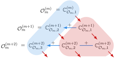
Figure 1: Diagrammatic representation of one way of using the recursion relations Eq. (10) and Eq. (11) to determine the full set of bias functions $\mathbb{C}^{(n)}_{\mathcal{O}_{m},\alpha}$ in the fluid expansion of a seed function $\mathcal{O}_{m}$. The red arrows indicate the use of the fluid recursion Eq. (11), while the blue arrows indicate the use of the completeness relation Eq. (10). Thus, the terms in the red shading ($\alpha<n-m+1$) are determined by the fluid recursion Eq. (11) and the terms in the blue shading ($\alpha=n-m+1$) are determined by the completeness relation Eq. (10).

III Bases for bias functions

Since we have formally done the integral over $t^{\prime}$ in Eq. (8), one might wonder where in Eq. (9) the non-local-in-time effect has gone. Comparing Eq. (9) to the local-in-time expression

$$\delta^{(n)}_{g,\text{loc}}(\vec{x},t)=\sum_{\mathcal{O}_{m}}c_{\mathcal{O}_{m}}(t)\,\mathcal{O}_{m}^{(n)}(\vec{x},t)\ ,$$ (12)

we see that the difference is in the basis functions of the expansion (which as we will discuss below control the possible functional forms of the clustering signals), since Eq. (9) is equivalent to Eq. (12) under the restriction that, for all $\alpha$, $c_{\mathcal{O}_{m},\alpha}(t)=c_{\mathcal{O}_{m}}(t)$.

We can therefore return to the main question posed by this Letter: is it possible to directly measure the effects of non-locality in time on galaxy clustering? In our perturbative description, this is equivalent to the the following mathematical question: does the basis for the non-local-in-time expansion Eq. (9) span a larger space than the basis for the local-in-time expansion Eq. (12)? The answer, as we will show below, is yes.

Let us start by noticing that, at a given order $n$, the set of bias functions $\mathbb{C}^{(n)}_{\mathcal{O}_{m},\alpha}$ is in general not linearly independent (once expressed as functionals of the linear dark-matter density $\delta^{(1)}$). As shown in D’Amico et al. (2022c), the non-local-in-time and local-in-time expansions are indeed equivalent up to fourth order in perturbations. However, from the findings of this Letter, this seems to simply be a consequence of expanding to low orders in perturbation theory where there are too few independent spatially local and Galilean invariant functional forms available, since non-locality-in-time is generically expected in the bias expansion Senatore (2015).

To find the fifth-order functions, we form the set $\{\mathcal{O}_{m}\}$ by finding all rotationally invariant contractions of $r_{ij}$ and $p_{ij}$ up to fifth order. Writing the first few terms, we have $\{\mathcal{O}_{m}\}=\{\delta,\theta,\delta^{2},\delta\theta,\theta^{2},r^{2},rp,p^{2},\dots\}$, and overall there are $63$ contractions with up to five factors. We then find the functions $\mathbb{C}_{\mathcal{O}_{m},\alpha}^{(n)}$ for $n\leq 5$ either by expanding $\vec{x}_{\rm fl}$ as in Eq. (LABEL:omordern), or, equivalently, using the recursion relations Eq. (10) and Eq. (11). After this, there are $151$ bias functions for $n=5$, and, for example, $88$ bias functions for $n=4$. We provide all of the Fourier-space kernels relevant for the fifth-order expansion in an associated ancillary file.

As mentioned above, though, not all of these functions are linearly independent, in the sense that

$$\sum_{\mathcal{O}_{m}}\sum_{\alpha=1}^{n-m+1}d^{(n)}_{i,\mathcal{O}_{m},\alpha}\mathbb{C}^{(n)}_{\mathcal{O}_{m},\alpha}(\vec{x},t)=0\ ,$$ (13)

for some time-independent coefficients $d^{(n)}_{i,\mathcal{O}_{m},\alpha}$ for $i=1,\dots,N_{d}^{(n)}$, where $N_{d}^{(n)}\equiv\text{rank}[d^{(n)}]$ is the number of independent degeneracy equations. In particular, we find $N_{d}^{(5)}=122$, and D’Amico et al. (2022c) found $N_{d}^{(4)}=73$. Letting $N_{b}^{(n)}$ denote the number of basis elements at order $n$, this means that $N_{b}^{(5)}=29$ and $N_{b}^{(4)}=15$. We confirm all of the fifth-order degeneracy equations in the associated ancillary file.

Thus, one can solve the degeneracy equations Eq. (13) in terms of $N_{b}^{(n)}$ basis elements, which we denote generically as $\mathbb{E}^{(n)}_{j}(\vec{x},t)$ for $j=1,\dots,N_{b}^{(n)}$. Since this is a basis, all of the original functions can be written in terms of it, so we have

$$\mathbb{C}^{(n)}_{\mathcal{O}_{m},\alpha}(\vec{x},t)=\sum_{j=1}^{N_{b}^{(n)}}A^{(n)}_{\mathcal{O}_{m},\alpha,j}\,\mathbb{E}^{(n)}_{j}(\vec{x},t)\ ,$$ (14)

for some time-independent coefficients $A^{(n)}_{\mathcal{O}_{m},\alpha,j}$. Plugging Eq. (14) into Eq. (9) then gives

$$\delta_{g}^{(n)}(\vec{x},t)=\sum_{j=1}^{N_{b}^{(n)}}e^{(n)}_{j}(t)\mathbb{E}^{(n)}_{j}(\vec{x},t)\ ,$$ (15)

where $e^{(n)}_{j}(t)=\sum_{\mathcal{O}_{m}}\sum_{\alpha=1}^{n-m+1}c_{\mathcal{O}_{m},\alpha}(t)A^{(n)}_{\mathcal{O}_{m},\alpha,j}$. The coefficients $e_{j}(t)$ are called bias parameters, and we have now written the galaxy overdensity in terms of the minimal number of linearly independent functions.

IV Non-local-in-time bias in LSS

We now consider the basis of bias functions for the local-in-time expression Eq. (12). At fifth order, this expansion starts with $63$ terms, however, as before, not all of them are linearly independent. We find $37$ independent degeneracy equations, and hence $26$ independent functions for the local-in-time bias expansion at fifth order. Indeed, this is three less than the non-local-in-time expansion, and hence the galaxy-clustering signal at fifth order is sensitive to whether or not galaxies form on time scales of order Hubble.

We are now in a position to explicitly give the fifth-order basis derived for this Letter. To be more concrete, we can write the fifth-order galaxy expansion in a basis with 26 elements that are local in time, and three that are non-local in time. In this starting-from-time-locality (STL) basis, we explicitly write

$$\delta_{g}^{(5)}(\vec{x},t)=\sum_{j=1}^{29}\tilde{b}_{j}(t)\mathbb{L}^{(5)}_{j}(\vec{x},t)\ .$$ (16)

We choose the basis such that the elements with $j=1,\dots,26$ are a basis of the local expansion Eq. (12). Explicitly, we take $\mathbb{L}_{j}^{(5)}=\mathcal{O}_{m}^{(5)}$ with the corresponding $\mathcal{O}_{m}$ given by

$$\begin{split}&\{\delta,\theta,\delta\theta,\theta^{2},r^{2},rp,p^{2},\theta^{3},r^{2}p,rp^{2},p^{3},\\ &\quad r^{2}\theta,rp\theta,p^{2}\theta,rp^{3},rprp,rp^{2}\delta,r^{3}\delta^{2},\\ &\quad\delta^{5},r^{3}\theta,rp^{2}\theta,rp\delta\theta,r^{2}\theta^{2},rp\theta^{2},\delta\theta^{3},\theta^{4}\}\ ,\end{split}$$ (17)

for $j=1,\dots,26$. Thus, the non-locality in time is contained in the final three basis elements, which we take to be

$$\begin{split}\mathbb{L}_{27}^{(5)}=\mathbb{C}_{\delta,5}^{(5)}\ ,\quad\mathbb{L}_{28}^{(5)}=\mathbb{C}_{r^{2},4}^{(5)}\ ,\quad\mathbb{L}_{29}^{(5)}=\mathbb{C}_{p^{3},3}^{(5)}\ .\end{split}$$ (18)

Non-zero $\tilde{b}_{27}$, $\tilde{b}_{28}$, and $\tilde{b}_{29}$ can only come from non-local-in-time physics, so we call them non-local-in-time bias parameters.

Another, perhaps more natural, choice of basis functions is the so-called basis of descendants Angulo et al. (2015), where if $\mathbb{C}_{\mathcal{O}_{m},\alpha}^{(n)}$ is used at order $n$, then $\mathbb{C}_{\mathcal{O}_{m},\alpha+1}^{(n+1)}$ is used at order $n+1$. We write the fifth-order expansion in the basis of descendants as

$$\delta_{g}^{(5)}(\vec{x},t)=\sum_{j=1}^{29}b_{j}(t)\mathbb{B}^{(5)}_{j}(\vec{x},t)\ .$$ (19)

As shown in App. B, the first $15$ terms in Eq. (19) are determined by the fourth-order terms. That is, for $j=1,\dots,15$, the $b_{j}$ in Eq. (19) are the same as those in D’Amico et al. (2022c), and the basis functions are given by

$$\mathbb{B}_{j}^{(5)}=\mathbb{B}_{j}^{(4)}\Big{|}_{\mathbb{C}_{\mathcal{O}_{m},\alpha}^{(4)}\rightarrow\mathbb{C}_{\mathcal{O}_{m},\alpha}^{(5)}}$$ (20)

where the $\mathbb{B}_{j}^{(4)}$ are given explicitly in D’Amico et al. (2022c). For the new elements derived here, i.e. $j=16,\dots,29$, we have $\mathbb{B}_{j}^{(5)}=\mathbb{C}_{\mathcal{O}_{m},\alpha}^{(5)}$, where the indices $\mathcal{O}_{m},\alpha$ take the following values for the given $j$

𝒪m,α:δ,5δ2,4r2,4δ3,3r3,3r2δ,3δ4,2j:23242526272829𝒪m,α:r3δ,2r4,2δ5,1r5,1r4δ,1r3δ2,1p3,3.fragments fragmentsO𝑚,α:fragmentsδ,5fragmentsδ2,4fragmentsr2,4fragmentsδ3,3fragmentsr3,3fragmentsr2δ,3fragmentsδ4,2fragmentsj:23242526272829fragmentsO𝑚,α:fragmentsr3δ,2fragmentsr4,2fragmentsδ5,1fragmentsr5,1fragmentsr4δ,1fragmentsr3δ2,1fragmentsp3,3\normalsize\begin{tabular}[]{|c|c|c|c|c|c|c|c|}\hline\cr$j:$&16&17&18&19&20&21&22\\ \hline\cr$\mathcal{O}_{m},\alpha:$&$\delta,5$&$\delta^{2},4$&$r^{2},4$&$\delta^{3},3$&$r^{3},3$&$r^{2}\delta,3$&$\delta^{4},2$\\ \hline\cr\hline\cr\hline\cr$j:$&23&24&25&26&27&28&29\\ \hline\cr$\mathcal{O}_{m},\alpha:$&$r^{3}\delta,2$&$r^{4},2$&$\delta^{5},1$&$r^{5},1$&$r^{4}\delta,1$&$r^{3}\delta^{2},1$&$p^{3},3$\\ \hline\cr\end{tabular}\ .

:j16171819202122:j16171819202122 (21)

We also note that fifth order is the first time that $\partial_{i}v^{j}$ has to be used as a seed function to form a basis, for example through $\mathbb{C}^{(5)}_{p^{3},3}$ above. This is contrasted with the case at fourth order where $\partial_{i}\partial_{j}\Phi$ is enough D’Amico et al. (2022c).

Converting between the STL basis and the basis of descendants, we find the following expression for the non-local-in-time bias parameters and the basis-of-descendants bias parameters

$$\begin{split}&\tilde{b}_{27}=b_{1}-4b_{2}+6b_{3}-4b_{4}+90b_{8}-76b_{9}+b_{16}\ ,\\ &\tilde{b}_{28}=b_{18}-b_{9}\ ,\\ &\tilde{b}_{29}=-\frac{4b_{8}}{3}+\frac{4b_{9}}{3}-\frac{10b_{11}}{3}+\frac{7b_{20}}{3}+b_{29}\ .\end{split}$$ (22)

To see more quantitatively how the non-local-in-time bias parameters measure the time scale of galaxy formation, consider the expression Eq. (8) for the bias parameters. Assuming that the kernel $c_{\mathcal{O}_{m}}(t,t^{\prime})$ has support over a time scale of order $1/\omega$ and expanding around the local-in-time limit, we have

$$c_{\mathcal{O}_{m},\alpha}(t)\approx c_{\mathcal{O}_{m}}(t)\left(1+g_{\mathcal{O}_{m},\alpha}(t){\frac{H}{\omega}}+\dots\right)\ ,$$ (23)

where the $\dots$ represents terms higher order in $H/\omega$, and $g_{\mathcal{O}_{m},\alpha}(t)\sim{\cal{O}}(1)$. Since the non-local-in-time bias parameters $\tilde{b}_{27}$, $\tilde{b}_{28}$ and $\tilde{b}_{29}$ all vanish in the local-in-time limit, they are proportional to (at least) $H/\omega$. The size of the deviation from the first term, which is the local-in-time piece, is controlled by $H/\omega$: if there is a sizable deviation from the local-in-time limit, then $\omega\sim H$, and thus the time scale of the kernel $c_{\mathcal{O}_{m}}(t,t^{\prime})$ is of the order $1/H$. In our case, this happens if $\tilde{b}_{27}$, $\tilde{b}_{28}$, or $\tilde{b}_{29}$ are order unity. This in turn would mean that the formation of the observed population of galaxies has been affected by the state of the Universe up to a Hubble time ago, and thus that it has formed on a time scale on the order of the age of the Universe.

V Observable signatures

Until now, we have focused on the perturbative galaxy overdensity field itself. In large-scale structure analyses, we typically compare to data using correlation functions (or $n$-point functions if they contain $n$ fields) of the overdensity fields of various tracers. Thus, one way to measure the non-local-in-time effect that we have discovered in this Letter is in correlation functions. Since we found that this effect arises at fifth order in perturbations, the lowest order observables sensitive to it are the two-loop two-point function through

$$\langle\delta_{g_{1}}^{(5)}(\vec{x}_{1})\delta_{g_{2}}^{(1)}(\vec{x}_{2})\rangle\ ,$$ (24)

the two-loop three-point function through

$$\langle\delta_{g_{1}}^{(5)}(\vec{x}_{1})\delta_{g_{2}}^{(2)}(\vec{x}_{2})\delta_{g_{3}}^{(1)}(\vec{x}_{3})\rangle\ ,$$ (25)

the one-loop four-point function through

$$\langle\delta_{g_{1}}^{(5)}(\vec{x}_{1})\delta_{g_{2}}^{(1)}(\vec{x}_{2})\delta_{g_{3}}^{(1)}(\vec{x}_{3})\delta_{g_{4}}^{(1)}(\vec{x}_{4})\rangle\ ,$$ (26)

and the one-loop five-point function through

$$\langle\delta_{g_{1}}^{(5)}(\vec{x}_{1})\delta_{g_{2}}^{(2)}(\vec{x}_{2})\delta_{g_{3}}^{(1)}(\vec{x}_{3})\delta_{g_{4}}^{(1)}(\vec{x}_{4})\delta_{g_{5}}^{(1)}(\vec{x}_{5})\rangle\ ,$$ (27)

and the tree-level six-point function through

$$\langle\delta_{g_{1}}^{(5)}(\vec{x}_{1})\delta_{g_{2}}^{(1)}(\vec{x}_{2})\delta_{g_{3}}^{(1)}(\vec{x}_{3})\delta_{g_{4}}^{(1)}(\vec{x}_{4})\delta_{g_{5}}^{(1)}(\vec{x}_{5})\delta_{g_{6}}^{(1)}(\vec{x}_{6})\rangle\ ,$$ (28)

where we have used the subscript $g_{i}$ to denote possibly different tracer samples (each of which can have a different set of bias parameters), and we have taken all fields to be at the same time $t$ and dropped that argument to remove clutter.

As two explicit examples, consider the contributions to the two-loop two-point function Eq. (24) and the tree-level six-point function Eq. (27) for $g_{i}=g$ for $i=1,\dots,6$. Using the STL basis Eq. (16), we have the explicit non-local-in-time contributions

$$\sum_{j=27}^{29}\tilde{b}_{j}\langle\mathbb{L}_{j}^{(5)}(\vec{x}_{1})\delta^{(1)}_{g}(\vec{x}_{2})\rangle\ ,$$ (29)

$$\sum_{j=27}^{29}\tilde{b}_{j}\langle\mathbb{L}_{j}^{(5)}(\vec{x}_{1})\delta_{g}^{(1)}(\vec{x}_{2})\delta_{g}^{(1)}(\vec{x}_{3})\delta_{g}^{(1)}(\vec{x}_{4})\delta_{g}^{(1)}(\vec{x}_{5})\delta_{g}^{(1)}(\vec{x}_{6})\rangle\ ,$$

to the two-point and six-point functions respectively. As we have seen, these would not be present in the galaxy correlation functions if galaxies formed in a local-in-time way. This makes them concrete, direct, observable signatures of the formation time of galaxies.

Appendix A Proof of fluid recursion

As mentioned in the main text, we want to take $d/dt$ of Eq. (LABEL:omordern), which means that we will need to know $\partial_{t}\vec{x}_{\rm fl}(\vec{x},t,t^{\prime})$. To find that, we notice that by definition the fluid element satisfies the composition rule

$$\vec{x}_{\rm fl}\left(\vec{x}_{\rm fl}(\vec{x},t_{\rm in},t),t,t^{\prime}\right)=\vec{x}_{\rm fl}(\vec{x},t_{\rm in},t^{\prime})\ .$$ (30)

Since the right-hand side is independent of $t$, this implies

$$\frac{d}{dt}\vec{x}_{\rm fl}\left(\vec{x}_{\rm fl}(\vec{x},t_{\rm in},t),t,t^{\prime}\right)=0\ .$$ (31)

Using the chain rule, and

$$\frac{d}{dt}\vec{x}_{\rm fl}(\vec{x},t_{\rm in},t)=\frac{1}{a(t)}\vec{v}(\vec{x}_{\rm fl}(\vec{x},t_{\rm in},t),t)\ ,$$ (32)

which follows immediately from the definition of $\vec{x}_{\rm fl}$ Eq. (5), this implies

$$\begin{split}0&=\Big{[}\frac{\partial}{\partial t}\vec{x}_{\rm fl}(\vec{y},t,t^{\prime})+\\ &\hskip 28.90755pt\frac{v^{i}(\vec{y},t)}{a(t)}\frac{\partial}{\partial y^{i}}\vec{x}_{\rm fl}(\vec{y},t,t^{\prime})\Big{]}\Big{|}_{\vec{y}=\vec{x}_{\rm fl}(\vec{x},t_{\rm in},t)}\ .\end{split}$$ (33)

Since the initial $t_{\rm in}$ is arbitrary, we can take $t_{\rm in}=t$, which gives

$$\left(\frac{\partial}{\partial t}+\frac{v^{i}(\vec{x},t)}{a(t)}\frac{\partial}{\partial x^{i}}\right)\vec{x}_{\rm fl}(\vec{x},t,t^{\prime})=0\ .$$ (34)

This equation simply says that the convective derivative of the fluid element is zero, which makes intuitive sense since the convective derivative is defined to be along the fluid flow.

Now we take $d/dt$ of both sides of Eq. (LABEL:omordern). The right-hand side is simple, and we have (defining $D(t^{\prime},t)^{\alpha}_{m}\equiv(D(t^{\prime})/D(t))^{\alpha+m-1}$ to reduce clutter)

$$\frac{D(t)}{\dot{D}(t)}\frac{d}{dt}\sum_{\alpha=1}^{n-m+1}D^{\alpha}_{m}(t^{\prime},t)\mathbb{C}_{\mathcal{O}_{m},\alpha}^{(n)}(\vec{x},t)=$$ (35)

$$\hskip 14.45377pt\sum_{\alpha=1}^{n-m+1}D^{\alpha}_{m}(t^{\prime},t)(n-\alpha-m+1)\mathbb{C}_{\mathcal{O}_{m},\alpha}^{(n)}(\vec{x},t)\ ,$$

where we have used Eq. (7) for the time dependence of $\mathbb{C}_{\mathcal{O}_{m},\alpha}^{(n)}$.

On the left-hand side, we have

$$\frac{d}{dt}[\mathcal{O}_{m}(\vec{x}_{\rm fl}(\vec{x},t,t^{\prime}),t^{\prime})]^{(n)}=\left[\frac{d}{dt}\mathcal{O}_{m}(\vec{x}_{\rm fl}(\vec{x},t,t^{\prime}),t^{\prime})\right]^{(n)}$$

$$=\left[\frac{\partial}{\partial t}x_{\rm fl}^{i}(\vec{x},t,t^{\prime})\frac{\partial}{\partial y^{i}}\mathcal{O}_{m}(\vec{y},t^{\prime})\Big{|}_{\vec{y}=\vec{x}_{\rm fl}(\vec{x},t,t^{\prime})}\right]^{(n)}$$

$$=\left[-\frac{v^{j}(\vec{x},t)}{a(t)}\frac{\partial}{\partial x^{j}}x_{\rm fl}^{i}(\vec{x},t,t^{\prime})\frac{\partial}{\partial y^{i}}\mathcal{O}_{m}(\vec{y},t^{\prime})\Big{|}_{\vec{y}=\vec{x}_{\rm fl}(\vec{x},t,t^{\prime})}\right]^{(n)}$$

$$=\left[-\frac{v^{j}(\vec{x},t)}{a(t)}\frac{\partial}{\partial x^{i}}\mathcal{O}_{m}(\vec{x}_{\rm fl}(\vec{x},t,t^{\prime}),t^{\prime})\right]^{(n)}$$ (36)

$$=\frac{\dot{D}(t)}{D(t)}\left[\frac{\partial_{i}}{\partial^{2}}\theta(\vec{x},t)\frac{\partial}{\partial x^{i}}\mathcal{O}_{m}(\vec{x}_{\rm fl}(\vec{x},t,t^{\prime}),t^{\prime})\right]^{(n)}$$

$$=\frac{\dot{D}(t)}{D(t)}\sum_{\ell=m}^{n-1}\frac{\partial_{i}}{\partial^{2}}\theta^{(n-\ell)}(\vec{x},t)\frac{\partial}{\partial x^{i}}\left[\mathcal{O}_{m}(\vec{x}_{\rm fl}(\vec{x},t,t^{\prime}),t^{\prime})\right]^{(\ell)}\ ,$$

where we have used Eq. (34) to go from the second to third line, the chain rule to go from the third to fourth line, and the definition of $\theta$ from Eq. (1) in the fifth line. Now, we use Eq. (LABEL:omordern) to replace $\left[\mathcal{O}_{m}(\vec{x}_{\rm fl}(\vec{x},t,t^{\prime}),t^{\prime})\right]^{(\ell)}$ to get

$$\frac{D(t)}{\dot{D}(t)}\frac{d}{dt}[\mathcal{O}_{m}(\vec{x}_{\rm fl}(\vec{x},t,t^{\prime}),t^{\prime})]^{(n)}$$ (37)

$$=\sum_{\ell=m}^{n-1}\sum_{\alpha=1}^{\ell-m+1}D^{\alpha}_{m}(t^{\prime},t)\frac{\partial_{i}}{\partial^{2}}\theta^{(n-\ell)}(\vec{x},t)\partial_{i}\mathbb{C}^{(\ell)}_{\mathcal{O}_{m},\alpha}(\vec{x},t)$$

$$=\sum_{\alpha=1}^{n-m}D^{\alpha}_{m}(t^{\prime},t)\sum_{\ell=m+\alpha-1}^{n-1}\frac{\partial_{i}}{\partial^{2}}\theta^{(n-\ell)}(\vec{x},t)\partial_{i}\mathbb{C}^{(\ell)}_{\mathcal{O}_{m},\alpha}(\vec{x},t)$$

where we have simply changed the order of the sums between the second and third lines. Equating the coefficients of each power of $D(t^{\prime})$ in Eq. (35) and Eq. (37) then gives our recursion relation Eq. (11).

Appendix B Lower-order bias parameters

Here we show how bias parameters at fourth order appear automatically as biases at fifth order. For notational convenience, in this Appendix we will use $\Gamma$ as the combined index $\mathcal{O}_{m},\alpha$, as in $\mathbb{C}_{\Gamma}^{(n)}\equiv\mathbb{C}_{\mathcal{O}_{m},\alpha}^{(n)}$, and $\Gamma_{n}$ as the set of the relevant $\mathcal{O}_{m}$ and $\alpha$ at order $n$, as defined in the sum in Eq. (9). We start with the fifth-order degeneracy equations. It turns out, as we explicitly check in the ancillary file, that the full set of degeneracy equations satisfied by $\mathbb{C}^{(5)}_{\Gamma}$, Eq. (13) with $n=5$, can be put in the block form

$$\begin{split}0=\sum_{\Gamma\in\Gamma_{4}}d^{(4)}_{i,\Gamma}\mathbb{C}^{(5)}_{\Gamma}(\vec{x},t)+\sum_{\Gamma\in\Gamma_{5}\setminus\Gamma_{4}}\tilde{d}^{(5)}_{i,\Gamma}\mathbb{C}^{(5)}_{\Gamma}(\vec{x},t)\ ,\end{split}$$ (38)

for $i=1,\dots,N_{d}^{(5)}$, with $d^{(4)}_{i,\Gamma}=0$ for $i\in[N_{d}^{(4)}+1,N_{d}^{(5)}]$ and $\tilde{d}^{(5)}_{i,\Gamma}=0$ for $i\in[1,N_{d}^{(4)}]$. For $i=1,\dots,N_{d}^{(4)}$, the second term on the right-hand side of Eq. (38) vanishes, so the $\mathbb{C}^{(5)}_{\Gamma}$ with $\Gamma\in\Gamma_{4}$ satisfy the same equations as the fourth-order functions, Eq. (13) with $n=4$. Therefore we can write them in an analogous way to the $n=4$ case of Eq. (14), that is

$$\mathbb{C}^{(5)}_{\Gamma}(\vec{x},t)=\sum_{j=1}^{N_{b}^{(4)}}A^{(4)}_{\Gamma,j}\,\mathbb{E}^{(5)}_{j}(\vec{x},t)\ ,$$ (39)

for $\Gamma\in\Gamma_{4}$, with

$$\mathbb{E}_{j}^{(5)}\equiv\mathbb{E}_{j}^{(4)}\Big{|}_{\mathbb{C}_{\Gamma}^{(4)}\rightarrow\mathbb{C}_{\Gamma}^{(5)}}\ ,$$ (40)

for $j=1,\dots,N_{b}^{(4)}$. Said another way, since the $\mathbb{E}_{j}^{(4)}$ are just linear combinations of some $\mathbb{C}_{\Gamma}^{(4)}$, we define $\mathbb{E}_{j}^{(5)}$ for $j=1,\dots,N_{b}^{(4)}$ to be the same expressions as $\mathbb{E}_{j}^{(4)}$, but with $\mathbb{C}_{\Gamma}^{(4)}$ replaced with $\mathbb{C}_{\Gamma}^{(5)}$, i.e.

$$\begin{split}&\mathbb{E}_{j}^{(4)}(\vec{x},t)=\sum_{\Gamma\in\Gamma_{4}}\beta^{(4)}_{j,\Gamma}\mathbb{C}_{\Gamma}^{(4)}(\vec{x},t)\ ,\\ &\mathbb{E}_{j}^{(5)}(\vec{x},t)=\sum_{\Gamma\in\Gamma_{4}}\beta^{(4)}_{j,\Gamma}\mathbb{C}_{\Gamma}^{(5)}(\vec{x},t)\ ,\end{split}$$ (41)

for some coefficients $\beta^{(4)}_{j,\Gamma}$.

Now, the bias expansion at fifth order is

$$\delta_{g}^{(5)}(\vec{x},t)=\sum_{\Gamma\in\Gamma_{5}}c_{\Gamma}(t)\mathbb{C}_{\Gamma}^{(5)}(\vec{x},t)\ .$$ (42)

The sum above can be split into a sum over $\Gamma\in\Gamma_{4}$ and a sum over $\Gamma\in\Gamma_{5}\setminus\Gamma_{4}$. For the sum over $\Gamma_{4}$, we have

$$\sum_{\Gamma\in\Gamma_{4}}c_{\Gamma}(t)\mathbb{C}_{\Gamma}^{(5)}(\vec{x},t)=\sum_{j=1}^{N_{b}^{(4)}}e^{(4)}_{j}(t)\mathbb{E}^{(5)}_{j}(\vec{x},t)\ ,$$ (43)

where we have used Eq. (39) and the definition of $e_{j}^{(4)}(t)$ below Eq. (15). Thus, the degeneracy equations Eq. (38) ensure that it is exactly the fourth-order bias parameters $e_{j}^{(4)}(t)$ that appear in Eq. (43). Then, for the sum over $\Gamma\in\Gamma_{5}\setminus\Gamma_{4}$ in Eq. (42), one can solve for the remaining $N_{b}^{(5)}-N_{b}^{(4)}$ basis elements using the rest of the degeneracy equations in Eq. (38), and this will introduce the additional bias parameters that were not present at fourth order. Since this is true for generic bias parameters $e_{j}^{(4)}(t)$, it is true in particular for the basis of descendants bias parameters $b_{j}^{(4)}(t)$ in Eq. (19).

References

- Bondi and Gold (1948) H. Bondi and T. Gold, Mon. Not. Roy. Astron. Soc. 108, 252 (1948).
- Stebbins and Whitford (1948) J. Stebbins and A. E. Whitford, Astrophysical Journal 108, 413 (1948).
- Gamow (1954) G. Gamow, Astronomical Journal 59, 200 (1954).
- Gao et al. (2005) L. Gao, V. Springel, and S. D. M. White, Mon. Not. Roy. Astron. Soc. 363, L66 (2005), arXiv:astro-ph/0506510 .
- Croton et al. (2007) D. J. Croton, L. Gao, and S. D. M. White, Mon. Not. Roy. Astron. Soc. 374, 1303 (2007), arXiv:astro-ph/0605636 .
- Mao et al. (2018) Y.-Y. Mao, A. R. Zentner, and R. H. Wechsler, Mon. Not. Roy. Astron. Soc. 474, 5143 (2018), [Erratum: Mon.Not.Roy.Astron.Soc. 481, 3167 (2018)], arXiv:1705.03888 [astro-ph.CO] .
- Baumann et al. (2012) D. Baumann, A. Nicolis, L. Senatore, and M. Zaldarriaga, JCAP 1207, 051 (2012), arXiv:1004.2488 [astro-ph.CO] .
- Carrasco et al. (2012) J. J. M. Carrasco, M. P. Hertzberg, and L. Senatore, JHEP 09, 082 (2012), arXiv:1206.2926 [astro-ph.CO] .
- D’Amico et al. (2019) G. D’Amico, J. Gleyzes, N. Kokron, D. Markovic, L. Senatore, P. Zhang, F. Beutler, and H. Gil-Marn, (2019), arXiv:1909.05271 [astro-ph.CO] .
- Ivanov et al. (2019) M. M. Ivanov, M. Simonović, and M. Zaldarriaga, (2019), arXiv:1909.05277 [astro-ph.CO] .
- Colas et al. (2019) T. Colas, G. D’Amico, L. Senatore, P. Zhang, and F. Beutler, (2019), arXiv:1909.07951 [astro-ph.CO] .
- D’Amico et al. (2022a) G. D’Amico, M. Lewandowski, L. Senatore, and P. Zhang, (2022a), arXiv:2201.11518 [astro-ph.CO] .
- D’Amico et al. (2022b) G. D’Amico, Y. Donath, M. Lewandowski, L. Senatore, and P. Zhang, (2022b), arXiv:2206.08327 [astro-ph.CO] .
- Coles (1993) P. Coles, Mon. Not. Roy. Astron. Soc. 262, 1065 (1993).
- Fry and Gaztanaga (1993) J. N. Fry and E. Gaztanaga, Astrophys. J. 413, 447 (1993), arXiv:astro-ph/9302009 .
- Desjacques et al. (2018) V. Desjacques, D. Jeong, and F. Schmidt, Phys. Rept. 733, 1 (2018), arXiv:1611.09787 [astro-ph.CO] .
- McDonald and Roy (2009) P. McDonald and A. Roy, JCAP 0908, 020 (2009), arXiv:0902.0991 [astro-ph.CO] .
- Senatore (2015) L. Senatore, JCAP 1511, 007 (2015), arXiv:1406.7843 [astro-ph.CO] .
- D’Amico et al. (2022c) G. D’Amico, Y. Donath, M. Lewandowski, L. Senatore, and P. Zhang, (2022c), arXiv:2211.17130 [astro-ph.CO] .
- Camelio and Lombardi (2015) G. Camelio and M. Lombardi, Astron. Astrophys. 575, A113 (2015), arXiv:1501.03014 [astro-ph.CO] .
- Catelan et al. (2001) P. Catelan, M. Kamionkowski, and R. D. Blandford, Mon. Not. Roy. Astron. Soc. 320, L7 (2001), arXiv:astro-ph/0005470 .
- Hirata and Seljak (2004) C. M. Hirata and U. Seljak, Phys. Rev. D 70, 063526 (2004), [Erratum: Phys.Rev.D 82, 049901 (2010)], arXiv:astro-ph/0406275 .
- Lewandowski et al. (2015) M. Lewandowski, A. Perko, and L. Senatore, JCAP 1505, 019 (2015), arXiv:1412.5049 [astro-ph.CO] .
- Bragança et al. (2020) D. P. L. Bragança, M. Lewandowski, D. Sekera, L. Senatore, and R. Sgier, (2020), arXiv:2010.02929 [astro-ph.CO] .
- Goroff et al. (1986) M. H. Goroff, B. Grinstein, S. J. Rey, and M. B. Wise, Astrophys. J. 311, 6 (1986).
- Fry (1996) J. N. Fry, Astrophys. J. Lett. 461, L65 (1996).
- Tegmark and Peebles (1998) M. Tegmark and P. J. E. Peebles, Astrophys. J. Lett. 500, L79 (1998), arXiv:astro-ph/9804067 .
- Mirbabayi et al. (2015) M. Mirbabayi, F. Schmidt, and M. Zaldarriaga, JCAP 1507, 030 (2015), arXiv:1412.5169 [astro-ph.CO] .
- Angulo et al. (2015) R. Angulo, M. Fasiello, L. Senatore, and Z. Vlah, JCAP 1509, 029 (2015), arXiv:1503.08826 [astro-ph.CO] .