Channel Estimation for RIS-Aided MIMO Systems: A Partially Decoupled Atomic Norm Minimization Approach

Abstract

Channel estimation (CE) plays a key role in reconfigurable intelligent surface (RIS)-aided multiple-input multiple-output (MIMO) communication systems, while it poses a challenging task due to the passive nature of RIS and the cascaded channel structures. In this paper, a partially decoupled atomic norm minimization (PDANM) framework is proposed for CE of RIS-aided MIMO systems, which exploits the three-dimensional angular sparsity of the channel. In particular, PDANM partially decouples the differential angles at the RIS from other angles at the base station and user equipment, reducing the computational complexity compared with existing methods. A reweighted PDANM (RPDANM) algorithm is proposed to further improve CE accuracy, which iteratively refines CE through a specifically designed reweighing strategy. Building upon RPDANM, we propose an iterative approach named RPDANM with adaptive phase control (RPDANM-APC), which adaptively adjusts the RIS phases based on previously estimated channel parameters to facilitate CE, achieving superior CE accuracy while reducing training overhead. Numerical simulations demonstrate the superiority of our proposed approaches in terms of running time, CE accuracy, and training overhead. In particular, the RPDANM-APC approach can achieve higher CE accuracy than existing methods within less than 40 percent training overhead while reducing the running time by tens of times.

I Introduction

Reconfigurable intelligent surface (RIS), also known as intelligent reflecting surface (IRS) [1], is a metasurface equipped with integrated circuits. It is typically composed of passive reflecting elements whose phases can be adapted independently to the instantaneous channel state information by an intelligent controller [2]. By adapting the phases of the reflecting elements, RIS can alter its electromagnetic response to the incident signals, thus compensating for the severe propagation path loss or mitigating potential interference [3]. Since RIS only employs passive reflecting elements without the use of active radio-frequency (RF) chains, it is generally more energy-efficient and cost-effective than traditional active relays [4, 5]. In addition, the compact size of RIS components facilitates their mass deployment in various structures, such as billboards, windows, and building facades, etc. [3]. Due to its low cost, low power consumption, high flexibility, and the ability to reconfigure wireless propagation environments, RIS is considered a promising technology for next-generation wireless networks [2, 3, 4, 5, 6, 7, 8, 9].

To fully unleash the potential performance gains brought by RIS, channel estimation (CE) is crucial in RIS-aided communication systems but challenging in practice [9, 2]. Firstly, in RIS-aided communication systems, apart from the direct link between the base station (BS) and the user equipment (UE), the BS-to-RIS channel and the RIS-to-UE channel need to be estimated. Yet, the cascaded channel structure poses a challenge for effective CE. Secondly, since the passive reflecting elements of RIS are generally equipped with phase shifters only [2, 3], the signal processing capability of RIS is limited, making it impossible to transmit or receive training signals for CE. In addition, since a RIS typically consists of a large amount of elements, the number of channel parameters to be estimated increases substantially in RIS-aided systems, imposing extra challenges and leading to overwhelming training overhead.

In fact, CE for RIS-aided communication systems has been widely studied in the literature, e.g., [10, 11, 12, 13, 14, 15, 16]. In particular, various classical CE methods, such as least squares (LS), were applied to RIS-aided communication systems in the early stage. For instance, a CE scheme employing LS based on the minimum variance unbiased estimation criterion was designed in [10]. By exploiting the parallel factorization of the cascaded BS-RIS-UE channel, an iterative CE algorithm capitalizing alternating LS was proposed in [11]. However, the aforementioned CE methods often require a quantity of training overhead, depending on the size of RIS. To reduce the training overhead, compressed sensing (CS) technology has been applied to the CE for RIS-aided communication systems, which exploits the angular sparsity of the channel. For instance, in [12], the design of CE was formulated as a sparse signal recovery problem and was solved by classical CS methods, such as orthogonal matching pursuit (OMP) [17]. Also, for RIS-aided multiple-input multiple-output (MIMO) systems, a two-stage CE framework was proposed in [13], where the estimation of channel parameters is decomposed into two subproblems with each being formulated as an angle-of-arrival (AoA) estimation problem and being solved by the OMP. However, since existing CS-based methods assume that the channel angular parameters lie in a set of grid points, they suffer from the grid mismatch problem [18, 19] caused by the limited grid resolution, which leads to a low CE accuracy.

Most recently, CE methods based on atomic norm minimization (ANM) [19] have been developed for RIS-aided communication systems [14, 15, 16], which directly estimate the desired channel angular parameters in the continuous domain and thus improve the CE accuracy. Specifically, a two-stage CE method was proposed in [14], where the channel parameters were divided into two groups and estimated by the ANM in two stages, respectively. Unfortunately, a large amount of training overhead is required in the first stage to reduce the possible error propagating to the second stage. When the location information of the RIS and BS is available, the authors in [15] proposed to leverage the location information for enhancing the CE performance and for saving the training overhead. Besides, in [16], two one-stage ANM-based CE methods were proposed for RIS-aided MIMO communication systems, i.e., ANM with two-dimensional (2D) atoms (ANM-2D) and ANM with three-dimensional (3D) atoms (ANM-3D). Although ANM-3D is generally superior to ANM-2D due to its more accurate characterization of the angular structure of the channel, a large-scale semidefinite programming (SDP) problem is required to be solved in ANM-3D, which has an order of magnitude higher computational complexity than that of the ANM-2D. This motivates us to develop novel ANM-based CE approaches to reduce the computational complexity and improve CE accuracy.

In this paper, we first propose a partially decoupled ANM (PDANM) framework with reduced computational complexity compared to state-of-the-art approaches. Based on PDANM, an iterative algorithm called reweighted PDANM (RPDANM) that achieves improved CE accuracy is proposed. To further reduce the training overhead, we propose an RPDANM with adaptive phase control (RPDANM-APC) approach that realizes high-accuracy CE with low training overhead for RIS-aided MIMO systems. The contributions of the paper are summarized as follows:

• We propose a one-stage PDANM framework for CE of RIS-aided MIMO systems, which exploits the 3D angular structure of the considered channel in a partially decoupled manner. Specifically, we first derive an effective channel model, which resolves the inherent parameter ambiguity of the previous cascaded channel model and has a simpler structure. On this basis, we define the partially decoupled atomic norm (PDAN) and reformulate the considered CE problem as a PDANM problem, which decouples the 3D angular structure of the effective channel into two lower-dimensional angular structures. Moreover, we formulate an SDP problem to efficiently solve the PDANM problem and establish the conditional equivalence between them.

• We propose an iterative CE algorithm called RPDANM, which promotes the 3D angular sparsity over PDANM by approximately solving a rank minimization problem instead of its convex relaxation. Compared with PDANM, RPDANM enhances CE accuracy through a specifically designed atom reweighting strategy without introducing additional training overhead. In particular, each iteration of RPDANM can be regarded as solving a weighted PDANM (WPDANM) problem with adaptively updated weighting functions.

• To reduce training overhead and to facilitate CE, we consider the design of the RIS phase control matrix during the training phase. By adaptively adjusting the phases of the RIS while estimating the channel parameters via RPDANM, we propose an RPDANM-APC approach that achieves promising CE accuracy with a limited training overhead.

The rest of the paper is organized as follows. Section II presents the system model for the considered RIS-aided MIMO communication system and introduces the adopted channel sounding procedure and the channel model. Section III proposes an effective channel model and a PDANM framework with a computational complexity analysis. Section IV proposes a PDANM-based iterative algorithm called RPDANM. Section V proposes an RPDANM-based iterative CE approach named RPDANM-APC. Section VI provides numerical simulations to demonstrate the advantages of our proposed methods in terms of CE accuracy, running time, and training overhead. Conclusions are drawn in Section VII.

Notations: Lowercase and uppercase bold letters represent vectors and matrices, respectively. $\mathbb{C}$ denotes the set of complex numbers. $|\cdot|$ denotes the amplitude of a scalar. $\overline{\left(\cdot\right)}$, $\left(\cdot\right)^{T}$, $\left(\cdot\right)^{H}$, and $\left(\cdot\right)^{\dagger}$ denote the conjugate, transpose, Hermitian transpose, and Moore-Penrose pseudo inverse, respectively. $\mathrm{rank}(\mathbf{A})$, $\mathrm{tr}(\mathbf{A})$, and $\mathrm{col}(\mathbf{A})$ denote the rank, trace, and column space of matrix $\mathbf{A}$, respectively, and $\mathbf{A}\succeq\mathbf{0}$ means that $\mathbf{A}$ is a Hermitian positive semidefinite (PSD) matrix. $\mathrm{diag}(\mathbf{x})$ is a diagonal matrix with its main diagonal entries given by $\mathbf{x}$. The identity matrix of size $N$ is denoted as $\mathbf{I}_{N}$. $[\mathbf{x}]_{l}$ denotes the $l$-th entry of the vector $\mathbf{x}$, and $[\mathbf{X}]_{i,j}$ denotes the $(i,j)$-th entry of the matrix $\mathbf{X}$. $\left\|\cdot\right\|_{2}$ and $\left\|\cdot\right\|_{F}$ denote the $\ell_{2}$ norm and the Frobenius norm, respectively. $\otimes$ and $\diamond$ denote the Kronecker product and Khatri-Rao product (or column-wise Kronecker product), respectively, and $\mathrm{vec}\left(\cdot\right)$ denotes vectorization. $a\mod b$ denotes the remainder of dividing $a$ by $b$. $\mathbb{E}(\cdot)$ is the expectation operator. $\mathcal{CN}(\mu,\sigma^{2})$ denotes a complex Gaussian distribution whose mean is $\mu$ and variance is $\sigma^{2}$. For a $D$-dimensional ($D\geq 2$) tensor $\mathbf{T}=[\mathbf{T}_{1},\cdots,\mathbf{T}_{2N_{1}-1}]\in\mathbb{C}^{(2N_{1}-1)\times\cdots\times(2N_{D}-1)}$, where $\mathbf{T}_{n_{1}}\in\mathbb{C}^{1\times(2N_{2}-1)\times\cdots\times(2N_{D}-1)}$ with $n_{1}\in\{1,\cdots,2N_{1}-1\}$, a $D$-level Toeplitz matrix [20] is defined recursively as

$$\mathcal{T}_{\mathbf{N}}(\mathbf{T})=\begin{bmatrix}\mathcal{T}_{\mathbf{N}_{-1}}(\mathbf{T}_{N_{1}})&\mathcal{T}_{\mathbf{N}_{-1}}(\mathbf{T}_{N_{1}+1})&\cdots&\mathcal{T}_{\mathbf{N}_{-1}}(\mathbf{T}_{2N_{1}-1})\\ \mathcal{T}_{\mathbf{N}_{-1}}(\mathbf{T}_{N_{1}-1})&\mathcal{T}_{\mathbf{N}_{-1}}(\mathbf{T}_{N_{1}})&\cdots&\mathcal{T}_{\mathbf{N}_{-1}}(\mathbf{T}_{2N_{1}-2})\\ \vdots&\vdots&\ddots&\vdots\\ \mathcal{T}_{\mathbf{N}_{-1}}(\mathbf{T}_{1})&\mathcal{T}_{\mathbf{N}_{-1}}(\mathbf{T}_{2})&\cdots&\mathcal{T}_{\mathbf{N}_{-1}}(\mathbf{T}_{N_{1}})\end{bmatrix},$$

where $\mathbf{N}=[N_{1},\cdots,N_{D}]$ and $\mathbf{N}_{-1}=[N_{2},\cdots,N_{D}]$. In particular, a ($1$-level) Toeplitz matrix is defined as

$$\mathcal{T}_{N}(\mathbf{t})=\begin{bmatrix}t_{N}&t_{N+1}&\cdots&t_{2N-1}\\ t_{N-1}&t_{N}&\cdots&t_{2N-2}\\ \vdots&\vdots&\ddots&\vdots\\ t_{1}&t_{2}&\cdots&t_{N}\end{bmatrix},$$

where $\mathbf{t}=[t_{1},\cdots,t_{2N-1}]\in\mathbb{C}^{2N-1}$.

II System Model

II-A System Model

We consider a RIS-aided MIMO communication system, where a BS communicates with a UE with the help of a RIS while the direct BS-to-UE channel is blocked, as shown in Fig. 1. The BS, UE, and RIS are equipped with uniform linear arrays (ULAs) of $N_{\mathrm{B}}$, $N_{\mathrm{U}}$, and $N_{\mathrm{R}}$ elements, respectively. In the considered RIS-aided MIMO system, the BS transmits training sequences, the RIS adjusts its phases to steer the signal towards the UE, and the UE estimates the cascaded BS-RIS-UE channel based on the received signals.

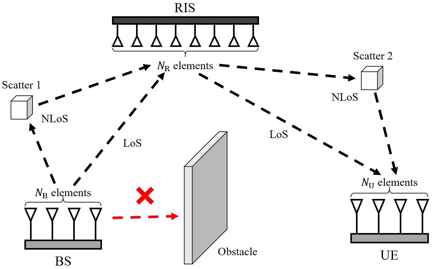
Figure 1: The considered RIS-aided MIMO communication system.

The detailed channel sounding procedure is introduced as follows. Following [14, 16], a slot-based channel sounding procedure is adopted in this paper, as illustrated in Fig. 2. In particular, a coherence time interval is divided into two periods for channel sounding and data transmission, respectively. The channel sounding period includes $B$ time slots and each time slot contains $M$ symbol durations. In the $b$-th time slot, $b\in\{1,\cdots,B\}$, the BS transmits $N_{\mathrm{B}}$ orthogonal training sequences, collected in $\mathbf{S}_{b}=[\mathbf{s}_{b1},\cdots,\mathbf{s}_{bN_{\mathrm{B}}}]^{T}\in\mathbb{C}^{N_{\mathrm{B}}\times M}$, satisfying $\mathbf{S}_{b}\mathbf{S}_{b}^{H}=P\mathbf{I}_{N_{\mathrm{B}}}$ with $P$ being the transmit power per antenna. The phase control vector for the RIS in the $b$-th time slot is denoted by $\boldsymbol{\omega}_{b}\in\mathbb{C}^{N_{\mathrm{R}}\times 1}$, of which each entry is unit-modulus, i.e., $\left|[\boldsymbol{\omega}_{b}]_{n_{\mathrm{R}}}\right|=1$, $\forall n_{\mathrm{R}}\in\{1,\cdots,N_{\mathrm{R}}\}$, since the passive reflecting elements in the RIS can only adjust their phases in practice [4, 14]. In the $b$-th training slot, the received signal at the UE is given by

$$\mathbf{Z}_{b}=\mathbf{H}^{b}_{\mathrm{BU}}\mathbf{S}_{b}+\mathbf{N}_{b},$$ (1)

where $\mathbf{H}^{b}_{\mathrm{BU}}\in\mathbb{C}^{N_{\mathrm{U}}\times N_{\mathrm{B}}}$ denotes the cascaded end-to-end channel between the BS and UE in the $b$-th time slot with $\boldsymbol{\omega}_{b}$ taken into account and $\mathbf{N}_{b}\in\mathbb{C}^{N_{\mathrm{U}}\times M}$ denotes the additive white Gaussian noise (AWGN) whose entries are independent and identically distributed (i.i.d.) following $\mathcal{CN}(0,\sigma^{2})$ with $\sigma^{2}$ being the noise variance. By exploiting the orthogonality of the training sequences, we right-multiply (1) by $\mathbf{S}_{b}^{H}/P$, which yields the processed signal as

$$\mathbf{Y}_{b}=\mathbf{H}^{b}_{\mathrm{BU}}+\mathbf{N}_{b}^{\prime},$$ (2)

where $\mathbf{N}_{b}^{\prime}=\frac{1}{P}\mathbf{N}_{b}\mathbf{S}_{b}^{H}\in\mathbb{C}^{N_{\mathrm{U}}\times N_{\mathrm{B}}}$ denotes a noise matrix with i.i.d. entries following $\mathcal{CN}(0,\frac{\sigma^{2}}{P})$. Then, the CE problem for the considered RIS-aided MIMO system in this paper is to estimate the cascaded channel $\mathbf{H}^{b}_{\mathrm{BU}}$ based on the processed signal $\mathbf{Y}_{b}$.

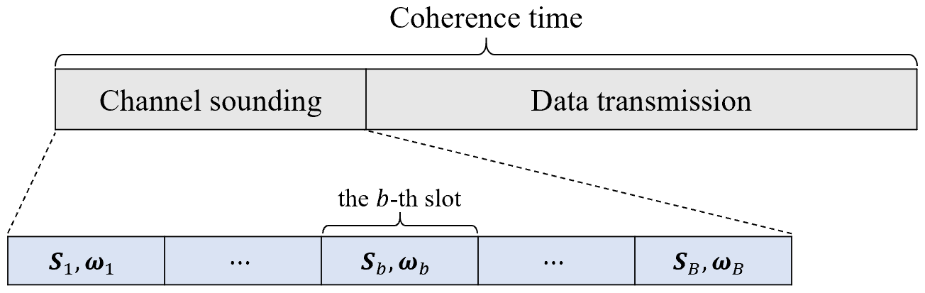
Figure 2: The adopted slot-based channel sounding procedure.

II-B Channel Model

In this paper, we assume a ray-tracing channel model [21] that has been commonly adopted in the RIS literature [13, 14, 15, 16]. We first define the steering vector of an $N$-element ULA with half-wavelength spacing as

$$\mathbf{a}_{N}(\theta)=\big{[}1,\mathrm{e}^{i\pi\cos\theta},\cdots,\mathrm{e}^{i\pi(N-1)\cos\theta}\big{]}^{T}\in\mathbb{C}^{N\times 1},$$ (3)

where $\theta$ denotes the steering angle. Now, the BS-to-RIS channel $\mathbf{H}_{\mathrm{BR}}\in\mathbb{C}^{N_{\mathrm{R}}\times N_{\mathrm{B}}}$ is modeled as

$$\mathbf{H}_{\mathrm{BR}} =\sum_{l_{\mathrm{BR}}=1}^{L_{\mathrm{BR}}}[\boldsymbol{\rho}_{\mathrm{BR}}]_{l_{\mathrm{BR}}}\mathbf{a}_{N_{\mathrm{R}}}([\boldsymbol{\phi}_{\mathrm{R}}]_{l_{\mathrm{BR}}})\mathbf{a}^{H}_{N_{\mathrm{B}}}([\boldsymbol{\theta}_{\mathrm{B}}]_{l_{\mathrm{BR}}})$$ (4)

$$=\mathbf{A}_{N_{\mathrm{R}}}(\boldsymbol{\phi}_{\mathrm{R}})\mathrm{diag}(\boldsymbol{\rho}_{\mathrm{BR}})\mathbf{A}^{H}_{N_{\mathrm{B}}}(\boldsymbol{\theta}_{\mathrm{B}}),$$

where $L_{\mathrm{BR}}$ denotes the number of paths between the BS and RIS, variables $[\boldsymbol{\theta}_{\mathrm{B}}]_{l_{\mathrm{BR}}},[\boldsymbol{\phi}_{\mathrm{R}}]_{l_{\mathrm{BR}}}\in[0,\pi]$, and $[\boldsymbol{\rho}_{\mathrm{BR}}]_{l_{\mathrm{BR}}}\in\mathbb{C}$ denote the angle-of-departure (AoD), AoA, and propagation path gain of the $l_{\mathrm{BR}}$-th path of the BS-to-RIS channel, respectively, $\mathbf{A}_{N_{\mathrm{B}}}(\boldsymbol{\theta}_{\mathrm{B}})=\big{[}\mathbf{a}_{N_{\mathrm{B}}}([\boldsymbol{\theta}_{\mathrm{B}}]_{1}),\cdots,\mathbf{a}_{N_{\mathrm{B}}}([\boldsymbol{\theta}_{\mathrm{B}}]_{L_{\mathrm{BR}}})\big{]}\in\mathbb{C}^{N_{\mathrm{B}}\times L_{\mathrm{BR}}}$, and $\mathbf{A}_{N_{\mathrm{R}}}(\boldsymbol{\phi}_{\mathrm{R}})=\big{[}\mathbf{a}_{N_{\mathrm{R}}}([\boldsymbol{\phi}_{\mathrm{R}}]_{1}),\cdots,\mathbf{a}_{N_{\mathrm{R}}}([\boldsymbol{\phi}_{\mathrm{R}}]_{L_{\mathrm{BR}}})\big{]}\in\mathbb{C}^{N_{\mathrm{R}}\times L_{\mathrm{BR}}}$. Similarly, the RIS-to-UE channel $\mathbf{H}_{\mathrm{RU}}\in\mathbb{C}^{N_{\mathrm{U}}\times N_{\mathrm{R}}}$ is modeled as

$$\mathbf{H}_{\mathrm{RU}} =\sum_{l_{\mathrm{RU}}=1}^{L_{\mathrm{RU}}}[\boldsymbol{\rho}_{\mathrm{RU}}]_{l_{\mathrm{RU}}}\mathbf{a}_{N_{\mathrm{U}}}([\boldsymbol{\phi}_{\mathrm{U}}]_{l_{\mathrm{RU}}})\mathbf{a}^{H}_{N_{\mathrm{R}}}([\boldsymbol{\theta}_{\mathrm{R}}]_{l_{\mathrm{RU}}})$$ (5)

$$=\mathbf{A}_{N_{\mathrm{U}}}(\boldsymbol{\phi}_{\mathrm{U}})\mathrm{diag}(\boldsymbol{\rho}_{\mathrm{RU}})\mathbf{A}^{H}_{N_{\mathrm{R}}}(\boldsymbol{\theta}_{\mathrm{R}}),$$

where $L_{\mathrm{RU}}$ denotes the number of paths between the RIS and UE, variables $[\boldsymbol{\theta}_{\mathrm{R}}]_{l_{\mathrm{RU}}},[\boldsymbol{\phi}_{\mathrm{U}}]_{l_{\mathrm{RU}}}\in[0,\pi]$, and $[\boldsymbol{\rho}_{\mathrm{RU}}]_{l_{\mathrm{RU}}}\in\mathbb{C}$ denote the AoD, AoA, and propagation path gain of the $l_{\mathrm{RU}}$-th path of the RIS-to-UE channel, respectively, $\mathbf{A}_{N_{\mathrm{R}}}(\boldsymbol{\theta}_{\mathrm{R}})=\big{[}\mathbf{a}_{N_{\mathrm{R}}}([\boldsymbol{\theta}_{\mathrm{R}}]_{1}),\cdots,\mathbf{a}_{N_{\mathrm{R}}}([\boldsymbol{\theta}_{\mathrm{R}}]_{L_{\mathrm{RU}}})\big{]}\in\mathbb{C}^{N_{\mathrm{R}}\times L_{\mathrm{RU}}}$, and $\mathbf{A}_{N_{\mathrm{U}}}(\boldsymbol{\phi}_{\mathrm{U}})=\big{[}\mathbf{a}_{N_{\mathrm{U}}}([\boldsymbol{\phi}_{\mathrm{U}}]_{1}),\cdots,\mathbf{a}_{N_{\mathrm{U}}}([\boldsymbol{\phi}_{\mathrm{U}}]_{L_{\mathrm{RU}}})\big{]}\in\mathbb{C}^{N_{\mathrm{U}}\times L_{\mathrm{RU}}}$. Now, the cascaded channel $\mathbf{H}^{b}_{\mathrm{BU}}\in\mathbb{C}^{N_{\mathrm{U}}\times N_{\mathrm{B}}}$ is given by

$$\mathbf{H}^{b}_{\mathrm{BU}} =\mathbf{H}_{\mathrm{RU}}\mathrm{diag}(\boldsymbol{\omega}_{b})\mathbf{H}_{\mathrm{BR}}$$ (6)

$$=\mathbf{A}_{N_{\mathrm{U}}}(\boldsymbol{\phi}_{\mathrm{U}})\mathrm{diag}(\boldsymbol{\rho}_{\mathrm{RU}})\mathbf{A}^{H}_{N_{\mathrm{R}}}(\boldsymbol{\theta}_{\mathrm{R}})\mathrm{diag}(\boldsymbol{\omega}_{b})\mathbf{A}_{N_{\mathrm{R}}}(\boldsymbol{\phi}_{\mathrm{R}})\mathrm{diag}(\boldsymbol{\rho}_{\mathrm{BR}})\mathbf{A}^{H}_{N_{\mathrm{B}}}(\boldsymbol{\theta}_{\mathrm{B}}).$$

It is observed from (6) that the cascaded channel $\mathbf{H}^{b}_{\mathrm{BU}}$ exhibits four-dimensional angular sparsity. Also, since $L_{\mathrm{BR}}$ and $L_{\mathrm{RU}}$ are small compared to the number of elements at the BS, UE, and RIS, it can be exploited to improve the efficiency of CE design for RIS-aided MIMO systems. Nevertheless, there are still a large number of channel parameters to be estimated to reconstruct $\mathbf{H}^{b}_{\mathrm{BU}}$. Even worse, they are severely coupled with each other, which motivates us to propose a decoupled CE method that maintains a high CE accuracy with a reduced computational complexity.

III Partially Decoupled ANM-based Channel Estimation Framework

In this section, we first reveal the inherent parameter ambiguity in the cascaded channel model and derive an effective channel model. Based on this model, we formulate the CE problem as a PDANM problem, which exploits the 3D angular sparsity of the effective channel in a partially decoupled manner. Since the problem at hand is intractable, we formulate an SDP problem that provides a lower bound for the original PDANM problem and is equivalent to PDANM under mild conditions. A detailed computational complexity analysis is further provided. In particular, the proposed PDANM-based CE framework serves as a building block for further improving CE accuracy and reducing training overhead in the following sections.

III-A Effective Channel Model

To begin with, we reveal the parameter ambiguity in the cascaded channel model in (6), as stated in the following proposition.

Proposition 1.

(Parameter Ambiguity) From a given $\mathbf{H}^{b}_{\mathrm{BU}}$, the parameters $\boldsymbol{\phi}_{\mathrm{R}}$, $\boldsymbol{\theta}_{\mathrm{R}}$, $\boldsymbol{\rho}_{\mathrm{BR}}$, and $\boldsymbol{\rho}_{\mathrm{RU}}$ in (6) cannot be uniquely identified, i.e., there are different sets of parameters satisfying

$$\mathbf{H}^{b}_{\mathrm{BU}} =\mathbf{A}_{N_{\mathrm{U}}}(\boldsymbol{\phi}_{\mathrm{U}})\mathrm{diag}(\boldsymbol{\rho}_{\mathrm{RU}})\mathbf{A}^{H}_{N_{\mathrm{R}}}(\boldsymbol{\theta}_{\mathrm{R}})\mathrm{diag}(\boldsymbol{\omega}_{b})\mathbf{A}_{N_{\mathrm{R}}}(\boldsymbol{\phi}_{\mathrm{R}})\mathrm{diag}(\boldsymbol{\rho}_{\mathrm{BR}})\mathbf{A}^{H}_{N_{\mathrm{B}}}(\boldsymbol{\theta}_{\mathrm{B}})$$ (7)

$$=\mathbf{A}_{N_{\mathrm{U}}}(\boldsymbol{\phi}_{\mathrm{U}})\mathrm{diag}(\boldsymbol{\rho}^{\prime}_{\mathrm{RU}})\mathbf{A}^{H}_{N_{\mathrm{R}}}(\boldsymbol{\theta}^{\prime}_{\mathrm{R}})\mathrm{diag}(\boldsymbol{\omega}_{b})\mathbf{A}_{N_{\mathrm{R}}}(\boldsymbol{\phi}^{\prime}_{\mathrm{R}})\mathrm{diag}(\boldsymbol{\rho}^{\prime}_{\mathrm{BR}})\mathbf{A}^{H}_{N_{\mathrm{B}}}(\boldsymbol{\theta}_{\mathrm{B}}),$$

where $\boldsymbol{\rho}^{\prime}_{\mathrm{RU}}\neq\boldsymbol{\rho}_{\mathrm{RU}}$, $\boldsymbol{\theta}^{\prime}_{\mathrm{R}}\neq\boldsymbol{\theta}_{\mathrm{R}}$, $\boldsymbol{\phi}^{\prime}_{\mathrm{R}}\neq\boldsymbol{\phi}_{\mathrm{R}}$, and $\boldsymbol{\rho}^{\prime}_{\mathrm{BR}}\neq\boldsymbol{\rho}_{\mathrm{BR}}$.

Proof.

See Appendix A. ∎

Proposition 1 reveals the parameter ambiguity in $\mathbf{H}^{b}_{\mathrm{BU}}$, which motivates the following effective channel model. Inserting (6) into (2) and vectorizing $\mathbf{Y}_{b}$, we have

$$\mathbf{y}_{b} =\mathrm{vec}(\mathbf{Y}_{b})=\mathrm{vec}\big{(}\mathbf{H}_{\mathrm{RU}}\mathrm{diag}(\boldsymbol{\omega}_{b})\mathbf{H}_{\mathrm{BR}}\big{)}+\mathrm{vec}(\mathbf{N}_{b}^{\prime})$$ (8)

$$\mathop{=}\limits^{\left(\mathrm{a}\right)}(\mathbf{H}_{\mathrm{BR}}^{T}\diamond\mathbf{H}_{\mathrm{RU}})\boldsymbol{\omega}_{b}+\mathbf{n}_{b}$$

$$\mathop{=}\limits^{\left(\mathrm{b}\right)}\big{[}\overline{\mathbf{A}_{N_{\mathrm{B}}}(\boldsymbol{\theta}_{\mathrm{B}})}\otimes\mathbf{A}_{N_{\mathrm{U}}}(\boldsymbol{\phi}_{\mathrm{U}})\big{]}\big{[}\mathrm{diag}(\boldsymbol{\rho}_{\mathrm{BR}})\otimes\mathrm{diag}(\boldsymbol{\rho}_{\mathrm{RU}})\big{]}\big{[}\mathbf{A}^{T}_{N_{\mathrm{R}}}(\boldsymbol{\phi}_{\mathrm{R}})\diamond\mathbf{A}^{H}_{N_{\mathrm{R}}}(\boldsymbol{\theta}_{\mathrm{R}})\big{]}\boldsymbol{\omega}_{b}+\mathbf{n}_{b},$$

where $\left(\mathrm{a}\right)$ and $\left(\mathrm{b}\right)$ in (8) are obtained by exploiting the properties of Kronecker and Khatri-Rao product [24], respectively, and $\mathbf{n}_{b}=\mathrm{vec}(\mathbf{N}_{b}^{\prime})\in\mathbb{C}^{N_{\mathrm{U}}N_{\mathrm{B}}\times 1}$. Furthermore, to resolve the parameter ambiguity illustrated in Proposition 1, we define the effective path gains as $\boldsymbol{\rho}_{\mathrm{BU}}=\boldsymbol{\rho}_{\mathrm{BR}}\otimes\boldsymbol{\rho}_{\mathrm{RU}}\in\mathbb{C}^{L_{\mathrm{BR}}L_{\mathrm{RU}}\times 1}$ and the differential angles $\boldsymbol{\psi}_{\mathrm{R}}$ at the RIS as follows:

$$\boldsymbol{\psi}_{\mathrm{R}}=\big{\{} [\boldsymbol{\psi}_{\mathrm{R}}]_{l_{\mathrm{BU}}}\in[0,\pi]:\cos([\boldsymbol{\psi}_{\mathrm{R}}]_{l_{\mathrm{BU}}})=\big{[}\cos([\boldsymbol{\theta}_{\mathrm{R}}]_{l_{\mathrm{RU}}})-\cos([\boldsymbol{\phi}_{\mathrm{R}}]_{l_{\mathrm{BR}}})\big{]}\mod 1,$$ (9)

$$l_{\mathrm{BR}}=1,\cdots,L_{\mathrm{BR}},\ l_{\mathrm{RU}}=1,\cdots,L_{\mathrm{RU}},l_{\mathrm{BU}}=(l_{\mathrm{BR}}-1)L_{\mathrm{RU}}+l_{\mathrm{RU}}\big{\}}.$$

Then, we define the effective channel $\mathbf{H}$ between the BS and UE as

$$\mathbf{H} =\mathbf{H}_{\mathrm{BR}}^{T}\diamond\mathbf{H}_{\mathrm{RU}}$$ (10)

$$=\big{[}\mathbf{A}_{N_{\mathrm{B}}}(-\boldsymbol{\theta}_{\mathrm{B}})\otimes\mathbf{A}_{N_{\mathrm{U}}}(\boldsymbol{\phi}_{\mathrm{U}})\big{]}\mathrm{diag}(\boldsymbol{\rho}_{\mathrm{BU}})\mathbf{A}^{H}_{N_{\mathrm{R}}}(\boldsymbol{\psi}_{\mathrm{R}})$$

$$=\sum_{l_{\mathrm{BR}}=1}^{L_{\mathrm{BR}}}\sum_{l_{\mathrm{RU}}=1}^{L_{\mathrm{RU}}}[\boldsymbol{\rho}_{\mathrm{BU}}]_{l_{\mathrm{BU}}}\big{[}\mathbf{a}_{N_{\mathrm{B}}}([-\boldsymbol{\theta}_{\mathrm{B}}]_{l_{\mathrm{BR}}})\otimes\mathbf{a}_{N_{\mathrm{U}}}([\boldsymbol{\phi}_{\mathrm{U}}]_{l_{\mathrm{RU}}})\big{]}\mathbf{a}^{H}_{N_{\mathrm{R}}}([\boldsymbol{\psi}_{\mathrm{R}}]_{l_{\mathrm{BU}}}),$$

where $l_{\mathrm{BU}}=(l_{\mathrm{BR}}-1)L_{\mathrm{RU}}+l_{\mathrm{RU}}$ and $\mathbf{A}_{N_{\mathrm{R}}}(\boldsymbol{\psi}_{\mathrm{R}})=\big{[}\mathbf{a}_{N_{\mathrm{R}}}([\boldsymbol{\psi}_{\mathrm{R}}]_{1}),\cdots,\mathbf{a}_{N_{\mathrm{R}}}([\boldsymbol{\psi}_{\mathrm{R}}]_{L_{\mathrm{BR}}L_{\mathrm{RU}}})\big{]}\in\mathbb{C}^{N_{\mathrm{R}}\times L_{\mathrm{BR}}L_{\mathrm{RU}}}$. With (10), the vectorized signal $\mathbf{y}_{b}$ in (8) can be rewritten as

$$\mathbf{y}_{b} =\mathbf{H}\boldsymbol{\omega}_{b}+\mathbf{n}_{b}.$$ (11)

By stacking the vectorized signals $\mathbf{y}_{b}$ in all the $B$ time slots into a received signal matrix, we have

$$\mathbf{Y}=\mathbf{H}\boldsymbol{\Omega}+\mathbf{N}\in\mathbb{C}^{N_{\mathrm{B}}N_{\mathrm{U}}\times B},$$ (12)

where $\boldsymbol{\Omega}=\big{[}\boldsymbol{\omega}_{1},\cdots,\boldsymbol{\omega}_{B}\big{]}\in\mathbb{C}^{N_{\mathrm{R}}\times B}$ denotes the RIS phase control matrix and $\mathbf{N}\in\mathbb{C}^{N_{\mathrm{B}}N_{\mathrm{U}}\times B}$ is the effective noise with i.i.d. entries following $\mathcal{CN}(0,\frac{\sigma^{2}}{P})$. Now, the CE problem of the considered RIS-aided MIMO system is to estimate the effective channel $\mathbf{H}$ from the received signal $\mathbf{Y}$ with the known phase control matrix $\boldsymbol{\Omega}$.

It is observed from (12) that the effective channel $\mathbf{H}$ is decoupled from the phases of RIS, which exhibits a simpler structure that is beneficial for CE. In particular, $\mathbf{H}$ exhibits a 3D angular sparsity with $L_{\mathrm{BR}}L_{\mathrm{RU}}$ number of effective paths in total, where the $\big{(}(l_{\mathrm{BR}}-1)L_{\mathrm{RU}}+l_{\mathrm{RU}}\big{)}$-th effective path corresponding to an effective path gain $[\boldsymbol{\rho}_{\mathrm{BR}}]_{l_{\mathrm{BR}}}[\boldsymbol{\rho}_{\mathrm{RU}}]_{l_{\mathrm{RU}}}$, an AoD $[\boldsymbol{\theta}_{\mathrm{B}}]_{l_{\mathrm{BR}}}$ from the BS, an AoA $[\boldsymbol{\phi}_{\mathrm{U}}]_{l_{\mathrm{RU}}}$ to the UE, and a differential angle $[\boldsymbol{\psi}_{\mathrm{R}}]_{(l_{\mathrm{BR}}-1)L_{\mathrm{RU}}+l_{\mathrm{RU}}}$ at the RIS. Besides, the effective channel model addresses the parameter ambiguity issue, thus benefiting channel parameters estimation.

Remark 1.

A model similar to (10) has been considered in [13] to separate the channel parameters at the BS and UE from those at the RIS and estimate them separately. Furthermore, [16] adopted the effective channel in (10) for CE without clarifying the reason. In contrast, in this paper, we explicitly illustrate the advantages of the effective channel model, i.e., simplifying the cascaded channel structure and avoiding parameter ambiguity, the latter of which seems to be ignored by existing papers. In particular, we analyze the structure of the effective channel model, which also inspires the PDANM method.

III-B Partially Decoupled ANM

Since the effective channel $\mathbf{H}$ exhibits a 3D angular sparsity, the considered CE problem can be formulated as a sparse optimization problem. In particular, the atomic norm [25] is a class of sparsity metrics capable of exploiting the channel structure. In the following, we introduce some basics of atomic set and ANM before proposing the PDANM framework for the CE problem.

If $\mathbf{H}$ can be represented as a linear combination of some elements in a set with some coefficients, we call this set an atomic set and this representation an atomic decomposition. The atomic norm [25] of $\mathbf{H}$ with respect to an atomic set is defined as the minimum sum of the absolute values of each coefficient among all its atomic decompositions regarding this atomic set. For example, the 2D atomic set [16] is defined as $\mathcal{A}_{\mathrm{2D}}=\Big{\{}\big{[}\mathbf{a}_{N_{\mathrm{B}}}(\theta)\otimes\mathbf{a}_{N_{\mathrm{U}}}(\phi)\big{]}\mathbf{b}^{H}:\theta,\phi\in[0,\pi],\|\mathbf{b}\|_{2}=1\Big{\}}$ and the corresponding 2D atomic norm of $\mathbf{H}$ is defined as

$$\|\mathbf{H}\|_{\mathcal{A}_{\mathrm{2D}}}=\inf\Big{\{}\sum_{l}|\rho_{l}|:\mathbf{H}=\sum_{l}\rho_{l}\big{[}\mathbf{a}_{N_{\mathrm{B}}}(\theta_{l})\otimes\mathbf{a}_{N_{\mathrm{U}}}(\phi_{l})\big{]}\mathbf{b}_{l}^{H},\theta_{l},\phi_{l}\in[0,\pi],\|\mathbf{b}_{l}\|_{2}=1\Big{\}},$$ (13)

which only exploits the 2D angular structure of the effective channel $\mathbf{H}$ but neglects its third-dimensional angular structure. To fully exploit the angular structure of the effective channel $\mathbf{H}$, [16] further proposed to vectorize $\mathbf{H}$ and define the 3D atomic set as $\mathcal{A}_{\mathrm{3D}}=\big{\{}\mathbf{a}_{N_{\mathrm{R}}}(\psi)\otimes\mathbf{a}_{N_{\mathrm{B}}}(\theta)\otimes\mathbf{a}_{N_{\mathrm{U}}}(\phi):\psi,\theta,\phi\in[0,\pi]\big{\}}$. Then, the corresponding 3D atomic norm of the vectorized effective channel $\mathrm{vec}(\mathbf{H})$ is defined as

$$\|\mathrm{vec}(\mathbf{H})\|_{\mathcal{A}_{\mathrm{3D}}}=\inf\Big{\{}\sum_{l}|\rho_{l}|:\mathrm{vec}(\mathbf{H})=\sum_{l}\rho_{l}\mathbf{a}_{N_{\mathrm{R}}}(\psi_{l})\otimes\mathbf{a}_{N_{\mathrm{B}}}(\theta_{l})\otimes\mathbf{a}_{N_{\mathrm{U}}}(\phi_{l}),\psi_{l},\theta_{l},\phi_{l}\in[0,\pi]\Big{\}},$$ (14)

which characterizes the structure of $\mathbf{H}$ more precisely than (13) due to exploring its 3D angular structure. Although (14) is intractable, $\|\mathrm{vec}(\mathbf{H})\|_{\mathcal{A}_{\mathrm{3D}}}$ can be calculated via solving the following SDP problem [20, 26]

$$\min_{t,\mathbf{T}}\frac{1}{2}t+\frac{1}{2N_{\mathrm{R}}N_{\mathrm{B}}N_{\mathrm{U}}}\mathrm{tr}(\mathcal{T}_{[N_{\mathrm{R}},N_{\mathrm{B}},N_{\mathrm{U}}]}(\mathbf{T})),\ \mathrm{s.t.}\begin{bmatrix}t&\mathrm{vec}(\mathbf{H})^{H}\\ \mathrm{vec}(\mathbf{H})&\mathcal{T}_{[N_{\mathrm{R}},N_{\mathrm{B}},N_{\mathrm{U}}]}(\mathbf{T})\end{bmatrix}\succeq\mathbf{0},$$ (15)

where $\mathcal{T}_{[N_{\mathrm{R}},N_{\mathrm{B}},N_{\mathrm{U}}]}(\mathbf{T})\in\mathbb{C}^{N_{\mathrm{R}}N_{\mathrm{B}}N_{\mathrm{U}}\times N_{\mathrm{R}}N_{\mathrm{B}}N_{\mathrm{U}}}$ is a $3$-level Toeplitz matrix, as defined in Section I.

Due to the vectorization of $\mathbf{H}$, a large-scale SDP problem needs to be solved for calculating $\|\mathrm{vec}(\mathbf{H})\|_{\mathcal{A}_{\mathrm{3D}}}$, which leads to prohibitively high computational complexity. For channels with only 2D angular structures, such as (4) and (5), a decoupled atomic norm and a decoupled ANM method was proposed in [27, 28], which reduces the computational complexity by decoupling the angular parameters in two different dimensions and solving a smaller-sized SDP problem. This motivates us to partially decouple the 3D angular parameters into two groups and reformulate the considered CE problem in (12) as a PDANM problem. For this purpose, we define the partially decoupled atomic set as $\mathcal{A}=\big{\{}\big{[}\mathbf{a}_{N_{\mathrm{B}}}(\theta)\otimes\mathbf{a}_{N_{\mathrm{U}}}(\phi)\big{]}\mathbf{a}^{H}_{N_{\mathrm{R}}}(\psi):\theta,\phi,\psi\in[0,\pi]\big{\}}$ and the PDAN as

$$\|\mathbf{H}\|_{\mathcal{A}}=\inf\Big{\{}\sum_{l}|\rho_{l}|:\mathbf{H}=\sum_{l}\rho_{l}\big{[}\mathbf{a}_{N_{\mathrm{B}}}(\theta_{l})\otimes\mathbf{a}_{N_{\mathrm{U}}}(\phi_{l})\big{]}\mathbf{a}^{H}_{N_{\mathrm{R}}}(\psi_{l}),\theta_{l},\phi_{l},\psi_{l}\in[0,\pi]\Big{\}}.$$ (16)

It is seen from the definitions of $\mathcal{A}$ and $\|\mathbf{H}\|_{\mathcal{A}}$ that they efficiently exploit the 3D angular structure of the effective channel. In addition, it is observed that $\|\mathrm{vec}(\mathbf{H})\|_{\mathcal{A}_{\mathrm{3D}}}=\|\mathbf{H}\|_{\mathcal{A}}$ by comparing (14) and (16). In particular, the calculation of $\|\mathbf{H}\|_{\mathcal{A}}$ can be realized by solving a smaller-size SDP problem than (15), as will be discussed below.

Similar to (14), (16) is an intractable problem, thus we formulate an SDP problem to calculate $\|\mathbf{H}\|_{\mathcal{A}}$ in the following theorem:

Theorem 1.

For a given effective channel $\mathbf{H}$, we have $\mathrm{SDP}(\mathbf{H})\leq\|\mathbf{H}\|_{\mathcal{A}}$, where $\mathrm{SDP}(\mathbf{H})$ is the optimal value of the following SDP problem:

$$\min_{\mathbf{t},\mathbf{T}}\frac{1}{2N_{\mathrm{R}}}\mathrm{tr}\big{(}\mathcal{T}_{N_{\mathrm{R}}}(\mathbf{t})\big{)}+\frac{1}{2N_{\mathrm{B}}N_{\mathrm{U}}}\mathrm{tr}\big{(}\mathcal{T}_{[N_{\mathrm{B}},N_{\mathrm{U}}]}(\mathbf{T})\big{)},\ \mathrm{s.t.}\begin{bmatrix}\mathcal{T}_{N_{\mathrm{R}}}(\mathbf{t})&\mathbf{H}^{H}\\ \mathbf{H}&\mathcal{T}_{[N_{\mathrm{B}},N_{\mathrm{U}}]}(\mathbf{T})\end{bmatrix}\succeq\mathbf{0}.$$ (17)

Furthermore, denote $\{\mathbf{t}^{*},\mathbf{T}^{*}\}$ as the optimizer of (17), then we have $\mathrm{SDP}(\mathbf{H})=\|\mathbf{H}\|_{\mathcal{A}}$ if all the following conditions are satisfied:

1. $\mathrm{rank}\big{(}\mathcal{T}_{N_{\mathrm{R}}}(\mathbf{t}^{*})\big{)}<N_{\mathrm{R}}$. It implies that $\mathcal{T}_{N_{\mathrm{R}}}(\mathbf{t}^{*})$ admits a Vandermonde decomposition [19, Theorem 11.5], i.e.,

   $$\mathcal{T}_{N_{\mathrm{R}}}(\mathbf{t}^{*}) =\sum_{l_{\mathrm{R}}=1}^{L_{\mathrm{R}}^{*}}[\mathbf{p}_{\mathrm{R}}^{*}]_{l_{\mathrm{R}}}\mathbf{a}_{N_{\mathrm{R}}}([\boldsymbol{\psi}_{\mathrm{R}}^{*}]_{l_{\mathrm{R}}})\mathbf{a}^{H}_{N_{\mathrm{R}}}([\boldsymbol{\psi}_{\mathrm{R}}^{*}]_{l_{\mathrm{R}}})$$ (18)

   $$=\mathbf{A}_{N_{\mathrm{R}}}(\boldsymbol{\psi}_{\mathrm{R}}^{*})\mathrm{diag}(\mathbf{p}_{\mathrm{R}}^{*})\mathbf{A}^{H}_{N_{\mathrm{R}}}(\boldsymbol{\psi}_{\mathrm{R}}^{*}),$$

   where $L_{\mathrm{R}}^{*}=\mathrm{rank}\big{(}\mathcal{T}_{N_{\mathrm{R}}}(\mathbf{t}^{*})\big{)}$ is the number of estimated differential angles, $[\boldsymbol{\psi}_{\mathrm{R}}^{*}]_{l_{\mathrm{R}}}$ is the $l_{\mathrm{R}}$-th estimated differential angle, $[\mathbf{p}_{\mathrm{R}}^{*}]_{l_{\mathrm{R}}}$ is the amplitude of the $l_{\mathrm{R}}$-th estimated path gain, and $\mathbf{A}_{N_{\mathrm{R}}}(\boldsymbol{\psi}_{\mathrm{R}}^{*})=\big{[}\mathbf{a}_{N_{\mathrm{R}}}([\boldsymbol{\psi}_{\mathrm{R}}^{*}]_{1}),\cdots,\mathbf{a}_{N_{\mathrm{R}}}([\boldsymbol{\psi}_{\mathrm{R}}^{*}]_{L_{\mathrm{R}}^{*}})\big{]}$ is a full column rank matrix.

2. $\mathcal{T}_{[N_{\mathrm{B}},N_{\mathrm{U}}]}(\mathbf{T}^{*})$ admits a 2-level Vandermonde decomposition [20], i.e.,

   $$\mathcal{T}_{[N_{\mathrm{B}},N_{\mathrm{U}}]}(\mathbf{T}^{*}) =\sum_{l_{\mathrm{BU}}=1}^{L_{\mathrm{BU}}^{*}}[\mathbf{p}_{\mathrm{BU}}^{*}]_{l_{\mathrm{BU}}}\big{[}\mathbf{a}_{N_{\mathrm{B}}}([\boldsymbol{\theta}_{\mathrm{B}}^{*}]_{l_{\mathrm{BU}}})\otimes\mathbf{a}_{N_{\mathrm{U}}}([\boldsymbol{\phi}_{\mathrm{U}}^{*}]_{l_{\mathrm{BU}}})\big{]}$$ (19)

   $$\quad\qquad\cdot\big{[}\mathbf{a}_{N_{\mathrm{B}}}([\boldsymbol{\theta}_{\mathrm{B}}^{*}]_{l_{\mathrm{BU}}})\otimes\mathbf{a}_{N_{\mathrm{U}}}([\boldsymbol{\phi}_{\mathrm{U}}^{*}]_{l_{\mathrm{BU}}})\big{]}^{H}$$

   $$=\big{[}\mathbf{A}_{N_{\mathrm{B}}}(\boldsymbol{\theta}_{\mathrm{B}}^{*})\diamond\mathbf{A}_{N_{\mathrm{U}}}(\boldsymbol{\phi}_{\mathrm{U}}^{*})\big{]}\mathrm{diag}(\mathbf{p}_{\mathrm{BU}}^{*})\big{[}\mathbf{A}_{N_{\mathrm{B}}}(\boldsymbol{\theta}_{\mathrm{B}}^{*})\diamond\mathbf{A}_{N_{\mathrm{U}}}(\boldsymbol{\phi}_{\mathrm{U}}^{*})\big{]}^{H},$$

   where $L_{\mathrm{BU}}^{*}=\mathrm{rank}\big{(}\mathcal{T}_{[N_{\mathrm{B}},N_{\mathrm{U}}]}(\mathbf{T}^{*})\big{)}$ is the number of estimated AoD-AoA pairs, $[\boldsymbol{\theta}_{\mathrm{B}}^{*}]_{l_{\mathrm{BU}}}$ is the $l_{\mathrm{BU}}$-th estimated AoD, $[\boldsymbol{\phi}_{\mathrm{U}}^{*}]_{l_{\mathrm{BU}}}$ is the $l_{\mathrm{BU}}$-th estimated AoA, $[\mathbf{p}_{\mathrm{BU}}^{*}]_{l_{\mathrm{BU}}}$ is the amplitude of the $l_{\mathrm{BU}}$-th estimated path gain, $\mathbf{A}_{N_{\mathrm{B}}}(\boldsymbol{\theta}_{\mathrm{B}}^{*})=\big{[}\mathbf{a}_{N_{\mathrm{B}}}([\boldsymbol{\theta}_{\mathrm{B}}^{*}]_{1}),\cdots,\mathbf{a}_{N_{\mathrm{B}}}([\boldsymbol{\theta}_{\mathrm{B}}^{*}]_{L_{\mathrm{BU}}^{*}})\big{]}$, $\mathbf{A}_{N_{\mathrm{U}}}(\boldsymbol{\phi}_{\mathrm{U}}^{*})=\big{[}\mathbf{a}_{N_{\mathrm{U}}}([\boldsymbol{\phi}_{\mathrm{U}}^{*}]_{1}),\cdots,\mathbf{a}_{N_{\mathrm{U}}}([\boldsymbol{\phi}_{\mathrm{U}}^{*}]_{L_{\mathrm{BU}}^{*}})\big{]}$, and $\big{[}\mathbf{A}_{N_{\mathrm{B}}}(\boldsymbol{\theta}_{\mathrm{B}}^{*})\diamond\mathbf{A}_{N_{\mathrm{U}}}(\boldsymbol{\phi}_{\mathrm{U}}^{*})\big{]}$ is a full column rank matrix.

3. The matrix $\mathbf{C}=\big{[}\mathbf{A}_{N_{\mathrm{B}}}(\boldsymbol{\theta}_{\mathrm{B}}^{*})\diamond\mathbf{A}_{N_{\mathrm{U}}}(\boldsymbol{\phi}_{\mathrm{U}}^{*})\big{]}^{\dagger}\mathbf{H}{\mathbf{A}^{H}_{N_{\mathrm{R}}}(\boldsymbol{\psi}_{\mathrm{R}}^{*})}^{\dagger}$ has only one nonzero element per row or per column.

Proof.

See Appendix B. ∎

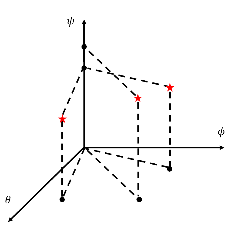
((a))

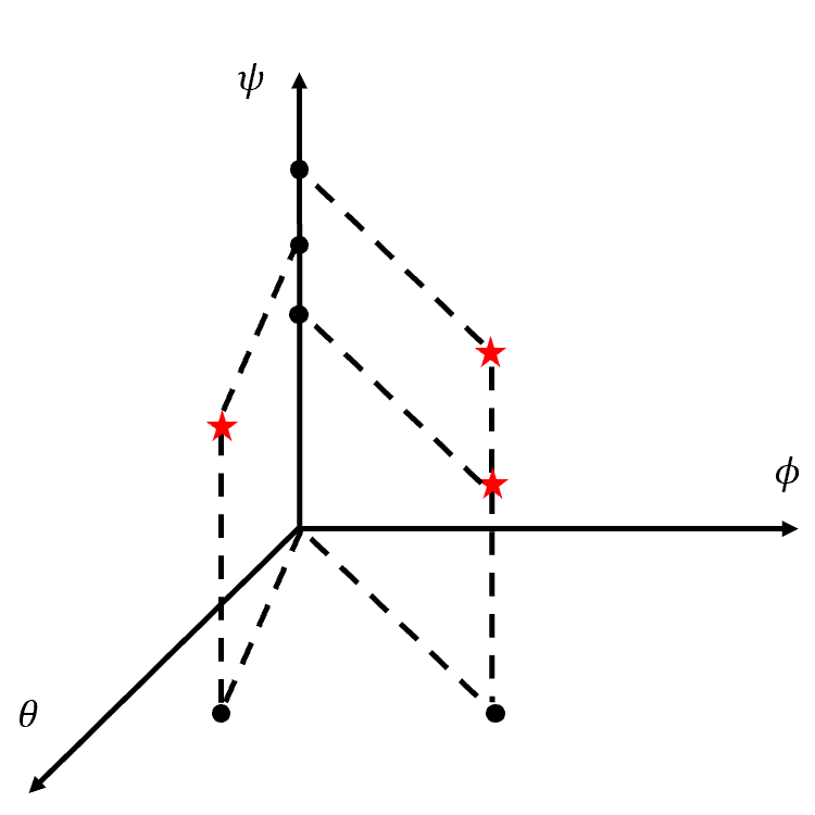
((b))

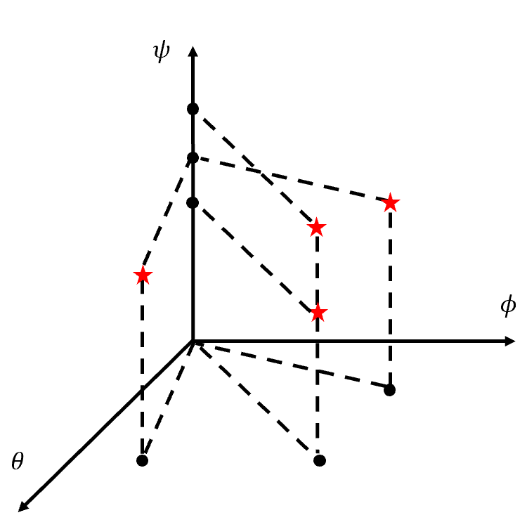
((c))

Figure 3: An example of groups of partially decoupled atoms in several cases, where the red pentagrams correspond to the partially decoupled atoms and the black dots denote their projections on the $\{\theta,\phi\}$ plane and $\psi$ axis. The three partially decoupled atoms in Fig. 3(a) are separable on the $\{\theta,\phi\}$ plane with $L_{\mathrm{R}}^{*}=2$ and $L_{\mathrm{BU}}^{*}=3$ and the three partially decoupled atoms in Fig. 3(b) are separable on the $\psi$ axis with $L_{\mathrm{R}}^{*}=3$ and $L_{\mathrm{BU}}^{*}=2$. The four partially decoupled atoms in Fig. 3(c) overlap on both the $\{\theta,\phi\}$ plane and the $\psi$ axis with $L_{\mathrm{R}}^{*}=L_{\mathrm{BU}}^{*}=3$.

Theorem 1 illustrates that $\mathrm{SDP}(\mathbf{H})$ genes as a lower bound for $\|\mathbf{H}\|_{\mathcal{A}}$ and proves the equivalence between (16) and (17) under some mild sufficient conditions. In particular, the first two conditions in Theorem 1 guarantee that a partially decoupled atomic decomposition of $\mathbf{H}$ can be obtained from the optimizer of (17), while the third condition implies that the corresponding partially decoupled atoms have either non-overlapping AoD-AoA pairs or non-overlapping differential angles. An example of groups of partially decoupled atoms is given in Fig. 3, where the partially decoupled atoms in Fig. 3(a) and Fig. 3(b) are separable on the $\{\theta,\phi\}$ plane or the $\psi$ axis and thus satisfy the conditions in Theorem 1, while those in Fig. 3(c) overlap on both the $\{\theta,\phi\}$ plane and the $\psi$ axis and thus do not satisfy the conditions in Theorem 1. In addition, we expect that $L_{\mathrm{R}}^{*}=L_{\mathrm{BU}}^{*}=L_{\mathrm{BR}}L_{\mathrm{RU}}$ holds in the general case, which means that both the numbers of estimated differential angles and estimated AoD-AoA pairs are equal to that of actual effective paths.

Furthermore, a more intuitive sufficient condition for the equivalence between (16) and (17) is that the effective channel paths are well separable in terms of differential angles, as stated in the following theorem:

Theorem 2.

Define the minimum sinusoidal interval of a set of angles $\boldsymbol{\psi}=[\psi_{1},\cdots,\psi_{K}]$ as

$$\Delta_{\boldsymbol{\psi}}=\inf_{\psi_{i},\psi_{j}:i\neq j}\{|\cos\psi_{i}-\cos\psi_{j}|,1-|\cos\psi_{i}-\cos\psi_{j}|\}.$$ (20)

If the actual differential angles $\boldsymbol{\psi}_{\mathrm{R}}$ satisfy that $\Delta_{\boldsymbol{\psi}_{\mathrm{R}}}>\frac{4}{N_{\mathrm{R}}}$, then we have $\mathrm{SDP}(\mathbf{H})=\|\mathbf{H}\|_{\mathcal{A}}$.

Proof.

See Appendix C. ∎

Under the condition that the actual differential angles $\boldsymbol{\psi}_{\mathrm{R}}$ are separable to a certain extent, Theorem 2 establishes the equivalence between (16) and (17). This condition generally holds in practice, as RIS usually consists of a large number of elements. Note that the condition stated in Theorem 2 pertains to the actual differential angles, while the conditions in Theorem 1 concern the estimated differential angles and AoD-AoA pairs. In conclusion, (17) provides a lower bound for $\|\mathbf{H}\|_{\mathcal{A}}$ and is equal to $\|\mathbf{H}\|_{\mathcal{A}}$ under two classes of mild conditions in Theorem 1 and Theorem 2, respectively.

Next, we formulate the considered CE problem as a PDANM problem, i.e., to treat $\mathbf{H}$ as an optimization variable and find an estimated channel matrix $\hat{\mathbf{H}}$ with the minimum PDAN. With Theorem 1 and Theorem 2, a solution to the PDANM problem can be obtained by solving the following problem:

$$\min_{\mathbf{t},\mathbf{T},\mathbf{H}} \frac{1}{2N_{\mathrm{R}}}\mathrm{tr}\big{(}\mathcal{T}_{N_{\mathrm{R}}}(\mathbf{t})\big{)}+\frac{1}{2N_{\mathrm{B}}N_{\mathrm{U}}}\mathrm{tr}\big{(}\mathcal{T}_{[N_{\mathrm{B}},N_{\mathrm{U}}]}(\mathbf{T})\big{)},$$ (21)

$$\mathrm{s.t.} \begin{bmatrix}\mathcal{T}_{N_{\mathrm{R}}}(\mathbf{t})&\mathbf{H}^{H}\\ \mathbf{H}&\mathcal{T}_{[N_{\mathrm{B}},N_{\mathrm{U}}]}(\mathbf{T})\end{bmatrix}\succeq\mathbf{0},\|\mathbf{Y}-\mathbf{H}\boldsymbol{\Omega}\|_{F}^{2}\leq\eta,$$

where $\eta$ is a given constant proportional to $\sigma^{2}$ [29]. Since (21) is an SDP problem, it can be solved by the interior-point method via an SDP solver, such as SDPT3 [30]. Our proposed framework is named PDANM since it essentially decouples the 3D angular structure of the effective channel into two low-dimensional angular structures, i.e., AoD-AoA pairs and differential angles.

Similarly, ANM-2D and ANM-3D find an $\hat{\mathbf{H}}$ with the minimum 2D atomic norm and 3D atomic norm for the CE by solving an SDP problem similar to (21), respectively. However, according to the analysis of the 2D atomic norm and 3D atomic norm above, ANM-2D does not fully exploit the 3D angular structure of $\mathbf{H}$, while ANM-3D needs to solve a large-scale SDP problem. Instead, the proposed PDANM framework not only fully exploits the 3D angular structure, but also reduces the computational complexity (to be illustrated in the next subsection), since the size of the PSD matrix in (17) is much smaller than that in (15). In addition, for the considered CE problem, it is difficult to define a fully decoupled atomic norm that is calculable.

III-C Complexity Analysis

In this subsection, we analyze the computational complexity of the proposed PDANM and compare it with the ANM-3D and ANM-2D in [16]. According to [31], the computational complexity of solving an SDP problem by the interior-point method is $\mathcal{O}\big{(}N_{\mathrm{1}}^{2}N_{\mathrm{2}}^{2.5}\big{)}$, where $N_{\mathrm{1}}$ is the variable size and $N_{\mathrm{2}}\times N_{\mathrm{2}}$ is the size of the PSD matrix. Since the dimension of the PSD matrix is $N_{\mathrm{B}}N_{\mathrm{U}}+N_{\mathrm{R}}$ and the variable size is on the order of $N_{\mathrm{B}}N_{\mathrm{U}}N_{\mathrm{R}}$ in (21), the computational complexity of PDANM is $\mathcal{O}\big{(}(N_{\mathrm{B}}N_{\mathrm{U}}N_{\mathrm{R}})^{2}(N_{\mathrm{B}}N_{\mathrm{U}}+N_{\mathrm{R}})^{2.5}\big{)}$, and the computational complexity of the ANM-2D approach and the ANM-3D can be derived by a similar analysis. In particular, we summarize the variable size, the matrix size, and the computational complexity of various ANM-based methods in Table I. For intuitive comparison, we calculate the ratio of complexity of ANM-2D and ANM-3D to that of PDANM, which are $\mathcal{O}\Big{(}\big{(}1+\frac{N_{\mathrm{R}}}{N_{\mathrm{B}}N_{\mathrm{U}}}\big{)}^{2}\Big{)}$ and $\mathcal{O}\Big{(}\big{(}\frac{N_{\mathrm{B}}N_{\mathrm{U}}N_{\mathrm{R}}}{N_{\mathrm{B}}N_{\mathrm{U}}+N_{\mathrm{R}}}\big{)}^{2.5}\Big{)}$, respectively. It is observed that the complexity of the proposed PDANM is lower than that of ANM-2D and is significantly lower than that of ANM-3D. Besides, in practice, the solution time of an SDP problem tends to depend heavily on the matrix size rather than the variable size. As a result, ANM-3D suffers a long running time due to the large size of the PSD matrix, as will be verified in Section VI.

TABLE I: Computational Complexity of ANM-based Methods

	Variable Size	Matrix Size	Computational Complexity
ANM-2D	$\mathcal{O}(N_{\mathrm{B}}N_{\mathrm{U}}N_{\mathrm{R}}+N_{\mathrm{R}}^{2})$	$N_{\mathrm{B}}N_{\mathrm{U}}+N_{\mathrm{R}}$	$\mathcal{O}\big{(}(N_{\mathrm{B}}N_{\mathrm{U}}N_{\mathrm{R}}+N_{\mathrm{R}}^{2})^{2}(N_{\mathrm{B}}N_{\mathrm{U}}+N_{\mathrm{R}})^{2.5}\big{)}$
ANM-3D	$\mathcal{O}(N_{\mathrm{B}}N_{\mathrm{U}}N_{\mathrm{R}})$	$N_{\mathrm{B}}N_{\mathrm{U}}N_{\mathrm{R}}$	$\mathcal{O}\big{(}(N_{\mathrm{B}}N_{\mathrm{U}}N_{\mathrm{R}})^{4.5}\big{)}$
PDANM	$\mathcal{O}(N_{\mathrm{B}}N_{\mathrm{U}}N_{\mathrm{R}})$	$N_{\mathrm{B}}N_{\mathrm{U}}+N_{\mathrm{R}}$	$\mathcal{O}\big{(}(N_{\mathrm{B}}N_{\mathrm{U}}N_{\mathrm{R}})^{2}(N_{\mathrm{B}}N_{\mathrm{U}}+N_{\mathrm{R}})^{2.5}\big{)}$

IV Reweighted PDANM Algorithm

To improve CE accuracy, in this section we propose an iterative algorithm named reweighted PDANM (RPDANM), which is inspired by the reweighted ANM algorithm proposed in our previous work [32, 33].

It is observed from (21) that PDANM promotes the sparsity of the effective channel by solving a trace minimization problem. A formulation that promotes sparsity more efficiently is the rank minimization problem obtained by substituting the trace in (21) for the rank:

$$\min_{\mathbf{t},\mathbf{T},\mathbf{H}} \frac{1}{2N_{\mathrm{R}}}\mathrm{rank}\big{(}\mathcal{T}_{N_{\mathrm{R}}}(\mathbf{t})\big{)}+\frac{1}{2N_{\mathrm{B}}N_{\mathrm{U}}}\mathrm{rank}\big{(}\mathcal{T}_{[N_{\mathrm{B}},N_{\mathrm{U}}]}(\mathbf{T})\big{)},$$ (22)

$$\mathrm{s.t.} \begin{bmatrix}\mathcal{T}_{N_{\mathrm{R}}}(\mathbf{t})&\mathbf{H}^{H}\\ \mathbf{H}&\mathcal{T}_{[N_{\mathrm{B}},N_{\mathrm{U}}]}(\mathbf{T})\end{bmatrix}\succeq\mathbf{0},\|\mathbf{Y}-\mathbf{H}\boldsymbol{\Omega}\|_{F}^{2}\leq\eta,$$

which is non-convex and NP-hard. In fact, (21) is the convex relaxation of (22). To further promote sparsity, we propose to approximately solve (22) via solving a set of SDP problems (see [32, 33] for details). The proposed algorithm is named RPDANM since the problem solved in each iteration is a weighted PDANM (WPDANM) problem with varying weighting matrices and functions, as will be detailed below.

To begin with, we define the weighted PDAN. For positive definite weighting matrices $\mathbf{W}_{\mathrm{BU}}\in\mathbb{C}^{N_{\mathrm{B}}N_{\mathrm{U}}\times N_{\mathrm{B}}N_{\mathrm{U}}}$ and $\mathbf{W}_{\mathrm{R}}\in\mathbb{C}^{N_{\mathrm{R}}\times N_{\mathrm{R}}}$, the weighting functions are defined as

$$w_{\mathrm{BU}}(\theta,\phi) =\Big{\{}\big{[}\mathbf{a}_{N_{\mathrm{B}}}(\theta)\otimes\mathbf{a}_{N_{\mathrm{U}}}(\phi)\big{]}^{H}\mathbf{W}_{\mathrm{BU}}\big{[}\mathbf{a}_{N_{\mathrm{B}}}(\theta)\otimes\mathbf{a}_{N_{\mathrm{U}}}(\phi)\big{]}\Big{\}}^{-1}\quad\text{and}$$ (23)

$$w_{\mathrm{R}}(\psi) =\big{[}\mathbf{a}^{H}_{N_{\mathrm{R}}}(\psi)\mathbf{W}_{\mathrm{R}}\mathbf{a}_{N_{\mathrm{R}}}(\psi)\big{]}^{-1},$$

respectively. Furthermore, we define the weighted partially decoupled atomic set as

$$\mathcal{A}^{w_{\mathrm{BU}},w_{\mathrm{R}}}=\Big{\{}w_{\mathrm{BU}}(\theta,\phi)^{\frac{1}{2}}w_{\mathrm{R}}(\psi)^{\frac{1}{2}}\big{[}\mathbf{a}_{N_{\mathrm{B}}}(\theta)\otimes\mathbf{a}_{N_{\mathrm{U}}}(\phi)\big{]}\mathbf{a}^{H}_{N_{\mathrm{R}}}(\psi):\theta,\phi,\psi\in[0,\pi]\Big{\}}$$ (24)

and the weighted PDAN of $\mathbf{H}$ as

$$\|\mathbf{H}\|_{\mathcal{A}^{w_{\mathrm{BU}},w_{\mathrm{R}}}} =\inf\Big{\{}\sum_{l}|\rho_{l}|:\mathbf{H}=\sum_{l}\rho_{l}w_{\mathrm{BU}}(\theta_{l},\phi_{l})^{\frac{1}{2}}w_{\mathrm{R}}(\psi_{l})^{\frac{1}{2}}$$ (25)

$$\qquad\ \cdot\big{[}\mathbf{a}_{N_{\mathrm{B}}}(\theta_{l})\otimes\mathbf{a}_{N_{\mathrm{U}}}(\phi_{l})\big{]}\mathbf{a}^{H}_{N_{\mathrm{R}}}(\psi_{l}),\theta_{l},\phi_{l},\psi_{l}\in[0,\pi]\Big{\}}$$

$$=\inf\Big{\{}\sum_{l}w_{\mathrm{BU}}(\theta_{l},\phi_{l})^{-\frac{1}{2}}w_{\mathrm{R}}(\psi_{l})^{-\frac{1}{2}}|\rho_{l}|:\mathbf{H}=\sum_{l}\rho_{l}$$

$$\qquad\ \cdot\big{[}\mathbf{a}_{N_{\mathrm{B}}}(\theta_{l})\otimes\mathbf{a}_{N_{\mathrm{U}}}(\phi_{l})\big{]}\mathbf{a}^{H}_{N_{\mathrm{R}}}(\psi_{l}),\theta_{l},\phi_{l},\psi_{l}\in[0,\pi]\Big{\}},$$

which is a generalization of the PDAN defined in (16) and degenerates to PDAN under specific weighting functions. Similar to (17), we formulate an SDP problem to calculate $\|\mathbf{H}\|_{\mathcal{A}^{w_{\mathrm{BU}},w_{\mathrm{R}}}}$ in the following theorem:

Theorem 3.

For a given effective channel $\mathbf{H}$, we have $\mathrm{SDP}_{\mathbf{W}_{\mathrm{R}},\mathbf{W}_{\mathrm{BU}}}(\mathbf{H})\leq\|\mathbf{H}\|_{\mathcal{A}^{w_{\mathrm{R}},w_{\mathrm{BU}}}}$ with $\mathrm{SDP}_{\mathbf{W}_{\mathrm{R}},\mathbf{W}_{\mathrm{BU}}}(\mathbf{H})$ being the optimal value of the following SDP problem:

$$\min_{\mathbf{t},\mathbf{T}}\frac{1}{2}\mathrm{tr}\big{(}\mathbf{W}_{\mathrm{R}}\mathcal{T}_{N_{\mathrm{R}}}(\mathbf{t})\big{)}+\frac{1}{2}\mathrm{tr}\big{(}\mathbf{W}_{\mathrm{BU}}\mathcal{T}_{[N_{\mathrm{B}},N_{\mathrm{U}}]}(\mathbf{T})\big{)},\ \mathrm{s.t.}\begin{bmatrix}\mathcal{T}_{N_{\mathrm{R}}}(\mathbf{t})&\mathbf{H}^{H}\\ \mathbf{H}&\mathcal{T}_{[N_{\mathrm{B}},N_{\mathrm{U}}]}(\mathbf{T})\end{bmatrix}\succeq\mathbf{0},$$ (26)

Furthermore, denote $\{\mathbf{t}^{*},\mathbf{T}^{*}\}$ as the optimizer of (26), then we have $\mathrm{SDP}_{\mathbf{W}_{\mathrm{R}},\mathbf{W}_{\mathrm{BU}}}(\mathbf{H})=\|\mathbf{H}\|_{\mathcal{A}^{w_{\mathrm{R}},w_{\mathrm{BU}}}}$ if the conditions 18), 19), and 3) in Theorem 1 hold.

Proof.

See Appendix D. ∎

By taking $\mathbf{W}_{\mathrm{BU}}=\frac{1}{N_{\mathrm{B}}N_{\mathrm{U}}}\mathbf{I}_{N_{\mathrm{B}}N_{\mathrm{U}}}$ and $\mathbf{W}_{\mathrm{R}}=\frac{1}{N_{\mathrm{R}}}\mathbf{I}_{N_{\mathrm{R}}}$, Theorem 1 is a special case of Theorem 3. Then, similar to PDANM, we treat $\mathbf{H}$ as an optimization variable and find an $\hat{\mathbf{H}}$ with the minimum weighted PDAN for the CE. With Theorem 3, the WPDANM problem can be effectively solved by solving an SDP problem:

$$\min_{\mathbf{t},\mathbf{T},\mathbf{H}} \frac{1}{2}\mathrm{tr}\big{(}\mathbf{W}_{\mathrm{R}}\mathcal{T}_{N_{\mathrm{R}}}(\mathbf{t})\big{)}+\frac{1}{2}\mathrm{tr}\big{(}\mathbf{W}_{\mathrm{BU}}\mathcal{T}_{[N_{\mathrm{B}},N_{\mathrm{U}}]}(\mathbf{T})\big{)},$$ (27)

$$\mathrm{s.t.} \begin{bmatrix}\mathcal{T}_{N_{\mathrm{R}}}(\mathbf{t})&\mathbf{H}^{H}\\ \mathbf{H}&\mathcal{T}_{[N_{\mathrm{B}},N_{\mathrm{U}}]}(\mathbf{T})\end{bmatrix}\succeq\mathbf{0},\|\mathbf{Y}-\mathbf{H}\boldsymbol{\Omega}\|_{F}^{2}\leq\eta,$$

which is a weighted version of (21). Due to the extra degrees of freedom introduced by weighting matrices, adopting appropriate weighting matrices will lead to a more accurate CE by (27) than (21).

Now, we propose an iterative RPDANM algorithm for CE of the considered RIS-aided MIMO system, which consists of solving a series of WPDANM problems with varying weighting matrices and functions. At the first iteration, we take initial weighting matrices $\mathbf{W}_{\mathrm{BU}}=\frac{1}{N_{\mathrm{B}}N_{\mathrm{U}}}\mathbf{I}_{N_{\mathrm{B}}N_{\mathrm{U}}}$ and $\mathbf{W}_{\mathrm{R}}=\frac{1}{N_{\mathrm{R}}}\mathbf{I}_{N_{\mathrm{R}}}$ and solve (27) to obtain the optimizer $\{\mathbf{t}^{*},\mathbf{T}^{*},\hat{\mathbf{H}}\}$ with $\hat{\mathbf{H}}$ being an estimate of the effective channel. Then, we update the weighting matrices as

$$\mathbf{W}_{\mathrm{BU}} =\big{(}\mathcal{T}_{[N_{\mathrm{B}},N_{\mathrm{U}}]}(\mathbf{T}^{*})+\epsilon\mathbf{I}_{N_{\mathrm{B}}N_{\mathrm{U}}}\big{)}^{-1}\quad\text{and}$$ (28)

$$\mathbf{W}_{\mathrm{R}} =\big{(}\mathcal{T}_{N_{\mathrm{R}}}(\mathbf{t}^{*})+\epsilon\mathbf{I}_{N_{\mathrm{R}}}\big{)}^{-1}$$

and solve (27) again to update $\{\mathbf{t}^{*},\mathbf{T}^{*},\hat{\mathbf{H}}\}$, where $\epsilon>0$ is a regularization parameter that guarantees the invertibility of matrices. To gradually approach a solution to (22), $\epsilon$ is halved after each iteration [32, 33]. This step is repeated until the difference between two adjacent $\hat{\mathbf{H}}$ is smaller than a given threshold or the maximum number of iterations is reached. It is worth mentioning that each iteration of our proposed RPDANM algorithm aims to solve a WPDANM problem, while the first iteration of RPDANM is equivalent to PDANM. In fact, the iterative process can be regarded as continuously selecting better weighting matrices according to the last CE to gradually refine the CE. The proposed RPDANM algorithm does not require additional training overhead, yet the iterative process incurs a higher computational complexity. Specifically, with $T$ denoting the number of iterations that is generally small, RPDANM is $T$ times slower than PDANM since each iteration has the same computational complexity as that of PDANM.

V RPDANM with Adaptive Phase Control Approach

Both PDANM and RPDANM follow the commonly adopted channel sounding procedure in the literature on RIS, as illustrated in Fig. 2. They both require a large number of training slots for realizing high CE accuracy, especially when the RIS consists of numerous elements. To facilitate low-overhead CE in the considered RIS-aided MIMO system, we consider the design of the phase control matrix $\boldsymbol{\Omega}$ for RIS during the training stage and propose an RPDANM with adaptive phase control (RPDANM-APC) approach for CE in this section.

Algorithm 1 Proposed RPDANM-APC Approach

0:  Noise variance $\sigma^{2}$, convergence threshold $\epsilon_{\mathbf{H}}$, initial number of training slots $B_{0}$, maximum number of training slots $B_{\max}$, phase control matrix $\boldsymbol{\Omega}\in\mathbb{C}^{N_{\mathrm{R}}\times B_{0}}$, regularization parameter $\epsilon=1$, weighting matrices $\mathbf{W}_{\mathrm{BU}}=\frac{1}{N_{\mathrm{B}}N_{\mathrm{U}}}\mathbf{I}_{N_{\mathrm{B}}N_{\mathrm{U}}}$ and $\mathbf{W}_{\mathrm{R}}=\frac{1}{N_{\mathrm{R}}}\mathbf{I}_{N_{\mathrm{R}}}$.

0:  Estimate of channel $\hat{\mathbf{H}}$, number of training slots $B$.

1:  Set $B=B_{0}$ and $K=0$.

2:  Send pilots in the first $B_{0}$ slots with the RIS phases set as each column of $\boldsymbol{\Omega}\in\mathbb{C}^{N_{\mathrm{R}}\times B_{0}}$, respectively, and collect the received data $\mathbf{Y}\in\mathbb{C}^{N_{\mathrm{B}}N_{\mathrm{U}}\times B_{0}}$.

3:   Solve the SDP problem in (27) to get its optimizer $\{\mathbf{t}^{*},\mathbf{T}^{*},\hat{\mathbf{H}}\}$ and $L^{*}_{K}=\mathrm{rank}(\mathcal{T}_{N_{\mathrm{R}}}(\mathbf{t}^{*}))$.

4:   Obtain $\boldsymbol{\psi}_{\mathrm{R}}^{*}$ from the Vandermonde decomposition of $\mathcal{T}_{N_{\mathrm{R}}}(\mathbf{t}^{*})$ as in (18) via root-MUSIC [34].

5:  while $B+L^{*}_{K}\leq B_{\max}$ do

6:     if $\epsilon>\frac{\sigma^{2}}{10}$ then

7:        Let $\epsilon=\frac{\epsilon}{2}$.

8:     end if

9:     Set $\hat{\mathbf{H}}_{\mathrm{last}}=\hat{\mathbf{H}}$, $B=B+L^{*}_{K}$.

10:     Send pilots in the following $L^{*}_{K}$ slots with the RIS phases set as each column of $\boldsymbol{\Omega}_{\mathrm{add}}=\mathbf{A}_{N_{\mathrm{R}}}(\boldsymbol{\psi}_{\mathrm{R}}^{*})\in\mathbb{C}^{N_{\mathrm{R}}\times L^{*}_{K}}$, respectively, and collect the received data $\mathbf{Y}_{\mathrm{add}}\in\mathbb{C}^{N_{\mathrm{B}}N_{\mathrm{U}}\times L^{*}_{K}}$.

11:     Update $\mathbf{W}_{\mathrm{BU}}$ and $\mathbf{W}_{\mathrm{R}}$ as (28), $\boldsymbol{\Omega}=\big{[}\boldsymbol{\Omega},\boldsymbol{\Omega}_{\mathrm{add}}\big{]}$, and $\mathbf{Y}=\big{[}\mathbf{Y},\mathbf{Y}_{\mathrm{add}}\big{]}$.

12:     Set $K=K+1$ and repeat Step 3 and Step 4.

13:     if $\frac{\hat{\mathbf{H}}-\hat{\mathbf{H}}_{\mathrm{last}}\|_{F}^{2}}{\|\hat{\mathbf{H}}_{\mathrm{last}}\|_{F}^{2}}<\sigma^{2}\epsilon_{\mathbf{H}}$ then

14:        break

15:     end if

16:  end while

In the following, we present the procedure of the proposed RPDANM-APC approach, including an initialization stage and an iteration stage, as summarized in Algorithm 1. The initialization stage includes Steps 1 to 4, where the initial training sequences are transmitted in Step 2 and the effective channel and its parameters are estimated in Steps 3 and 4. The iteration stage includes Steps 5 to 16, where the steps of setting RIS phases, sending pilot and collecting received data, and channel parameter estimation are performed in each iteration. Note that these steps are repeated until convergence or the upper bound of training overhead is reached. Specifically, $\epsilon$ is halved until smaller than a given threshold, e.g., $2^{-10}$. In each slot of an iteration, the RIS phases are set as the steering vector corresponding to each estimated differential angle for coherently combining the signal from a BS-to-RIS path to a RIS-to-UE path. In Step 12, additional training sequences are employed for updating the CE with the specially set RIS phases. Note that the number of slots used in each iteration is equal to the number of estimated differential angles in the last iteration such that all estimated differential angles are explored. The convergence of the algorithm is checked in Steps 13 to 15, where $\epsilon_{\mathbf{H}}$ is a given constant accusing for the tolerance of converge accuracy.

By iteratively updating the RIS phases, sending pilots, and performing CE, the proposed RPDANM-APC approach takes full advantage of the ability of RIS to reshape the wireless propagation environment. Since the phases of RIS elements are adaptively adjusted to match the estimated effective paths, the passive beamforming gain of RIS can be fully exploited to improve CE accuracy. Moreover, as only part of the angular space is searched during iterations, RPDANM-APC achieves a reduced training overhead compared to the PDANM and RPDANM methods. Note that the trade-off between training overhead and CE accuracy can be optimized by changing $B_{\max}$ and $\epsilon_{\mathbf{H}}$. The total number of training slots required by RPDANM-APC is $B=B_{0}+\sum_{k=0}^{K-1}L^{*}_{k}$ that is bounded by $B_{\max}$, where $K$ is the total number of iterations and $L^{*}_{k}$ is the number of estimated differential angles at the $k$-th iteration. Since the computational complexity of the root-MUSIC algorithm in Step 4 is $\mathcal{O}\big{(}N_{\mathrm{R}}^{3}\big{)}$, the computational complexity of RPDANM-APC mainly comes from solving SDP problems in Step 3, i.e., $\mathcal{O}\big{(}K(N_{\mathrm{B}}N_{\mathrm{U}}N_{\mathrm{R}})^{2}(N_{\mathrm{B}}N_{\mathrm{U}}+N_{\mathrm{R}})^{2.5}\big{)}$.

VI Numerical Simulations

VI-A Simulation Settings

In this section, we evaluate the performance of our proposed methods through numerical simulations. Unless otherwise stated, the default parameters are set as follows. We select $N_{\mathrm{B}}=4$, $N_{\mathrm{U}}=4$, $N_{\mathrm{R}}=16$, and $L_{\mathrm{BR}}=L_{\mathrm{RU}}=2$. All AoAs and AoDs are randomly and uniformly located in $[0,\pi]$ and all path gains are generated i.i.d. from $\mathcal{CN}(0,1)$. The signal-to-noise ratio (SNR) is defined as

$$\text{SNR}=10\log_{10}\frac{P}{\sigma^{2}},$$ (29)

which is set 30 dB as default. The convergence threshold is set $\epsilon_{\mathbf{H}}=10^{-3}$. As in [29], we set $\eta=\big{(}N_{\mathrm{B}}N_{\mathrm{U}}B+2\sqrt{N_{\mathrm{B}}N_{\mathrm{U}}B}\big{)}\sigma^{2}$ when solving a given SDP problem. For RPDANM, the maximum iteration number is 10. For RPDANM-APC, the initial and maximum number of training slots is $B_{0}=\frac{N_{\mathrm{R}}}{2}$ and $B_{\max}=N_{\mathrm{R}}$, respectively, while the number of training slots for all other methods is $N_{\mathrm{R}}$. Note that $B_{\max}$ is set to a large value here to observe the convergence performance of RPDANM-APC. In practice, $B_{\max}$ can be set to a small value to balance the required training overhead and CE accuracy. In addition, each entry of the (initial) phase control matrix $\boldsymbol{\Omega}$ is generated from the i.i.d. uniform distribution on a complex unit circle for all the considered methods, obeying the isotropy and incoherence properties in [35].

VI-B Channel Estimation Accuracy

In this subsection, we compare the CE accuracy of the proposed three methods to the state-of-the-art approaches, i.e., ANM-2D and ANM-3D, evaluated by the normalized mean square error (NMSE) that defined as

$$\text{NMSE}=\mathbb{E}\left(\frac{\|\hat{\mathbf{H}}-\mathbf{H}\|_{F}^{2}}{\|\mathbf{H}\|_{F}^{2}}\right).$$ (30)

An illustrative example is provided in Fig. 4, which depicts the NMSE of different methods versus the iteration index in a simulation. Among the single-step algorithms, we observe that PDANM significantly outperforms ANM-2D due to the exploitation of the 3D angular structure of the effective channel. Besides, an accuracy loss of PDANM compared to ANM-3D can be observed due to the conditional equivalence between the PDAN and the solved SDP problem, as stated in Theorem 1. Furthermore, the first iteration of RPDANM is equivalent to PDANM and thus they achieve the same accuracy. Besides, the CE accuracy of RPDANM is enhanced in subsequent iterations by continuously selecting better weighting matrices. In addition, the performance of RPDANM-APC is worse than that of RPDANM in the first iteration since few initial training slots are employed. However, as the number of training slots increases, the RPDANM-APC approach even outperforms RPDANM in terms of CE accuracy as it can exploit the ability of RIS to reshape wireless propagation.

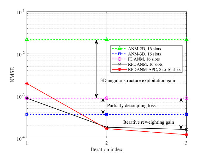
Figure 4: NMSE of different methods versus iteration index. Dashed lines denote one-step methods and solid lines denote iterative methods.

To comprehensively compare the performance of the proposed methods, Fig. 5 illustrates the NMSE of different methods versus the SNR. We set 9 different SNR levels in the range of [0 dB, 40 dB] and conduct 100 Monte Carlo experiments under each setting. It is observed that the PDANM is superior to ANM-2D due to the exploration of the 3D angular structure of the effective channel, but inferior to ANM-3D due to the accuracy loss caused by partially decoupling. By approximately solving a rank minimization problem via solving a series of WPDANM problems, RPDANM achieves a higher CE accuracy than PDANM. Furthermore, RPDANM-APC outperforms other methods when $\text{SNR}>20\ \mathrm{dB}$. The above simulation results demonstrate the excellent performance of our proposed methods, especially RPDANM and RPDANM-APC in terms of CE accuracy, consistent with our expectations and the example in Fig. 4.

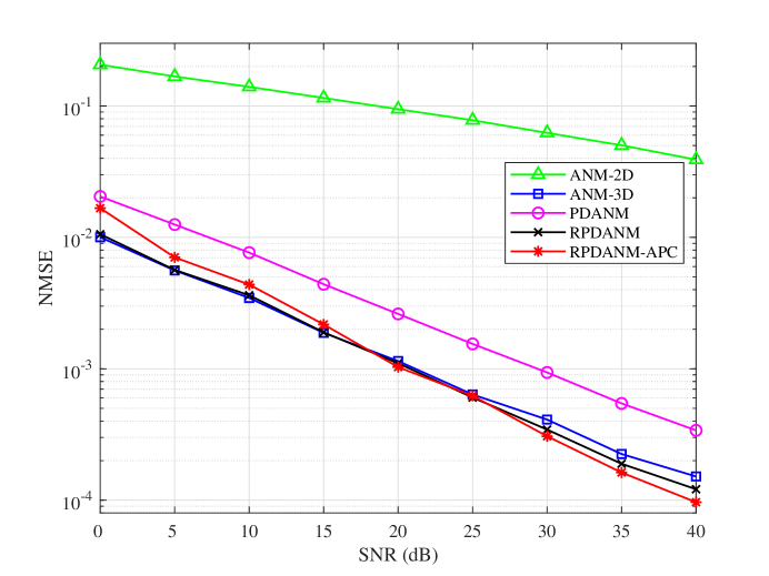
Figure 5: NMSE of different methods versus SNR.

VI-C Running Time

In this subsection, we compare the running time of different methods versus the size of RIS. For a convenient comparison, Fig. 6 depicts the ratios of running time of different methods with respect to our proposed PDANM approach versus RIS size, where the running time ratio of the PDANM approach is normalized to one unit. The size of RIS increases from 10 to 26 with 50 Monte Carlo simulations performed under each setting. It is observed that the running time of ANM-3D is tens or hundreds of times longer than that of other methods due to the requirement to solve a large-scale SDP problem. Besides, the running time of the proposed PDANM method is shorter than that of ANM-2D due to fewer involved optimization variables. These simulation results are consistent with our computational complexity analysis in Section III-C. Furthermore, the running time of both RPDANM and RPDANM-APC are less than 5 times that of PDANM since only a few iterations are required for convergence. In addition, as $N_{\mathrm{R}}$ increases, the running time of ANM-3D increases rapidly, while those of other methods ramp up slowly.

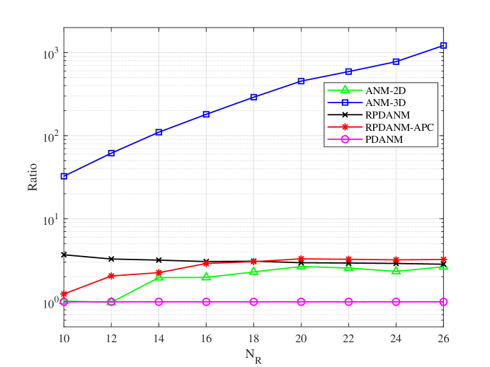
Figure 6: Running time ratios of different methods with respect to the benchmark versus the size of RIS.

VI-D Training Overhead

In this subsection, we compare the required training slots of different methods to illustrates the ability to save training overhead by the proposed RPDANM-APC approach. Fig. 7 depicts the NMSE of different methods versus the number of training slots, where a 64-element RIS is considered to ensure the clear presentation of the result. Under this setting, ANM-3D cannot be applied due to the exceedingly large size of the PSD matrix in the SDP problem to be solved. For RPDANM-APC, we select three different initial number of training slots to observe its performance, i.e., $B_{0}=8,12,16$ (corresponding to 2, 3, and 4 times the number of effective paths, respectively). We vary the number of training slots from 8 to 64 and conduct 100 Monte Carlo simulations under each setting to observe the performance of ANM-2D, PDANM, and RPDANM. Since the number of training slots employed by RPDANM-APC cannot be specified, we indirectly control it by varying $B_{\max}$ (or other parameters, e.g., $\epsilon_{\mathbf{H}}$) and observe the average number of training slots and the average NMSE of RPDANM-APC under different settings. It is seen that PDRANM-APC performs better than other methods within limited training overhead with appropriate $B_{0}$. Specifically, when $B_{0}=16$, RPDANM-APC achieves higher CE accuracy than RPDANM while saving more than $60\%$ training slots. In addition, when $B_{\max}$ is sufficiently large to ensure convergence of RPDANM-APC, increasing $B_{\max}$ can barely alter the required number of training slots.

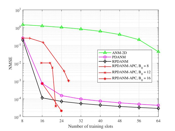
Figure 7: NMSE of different methods versus the number of training slots.

VI-E Selection of Initial Number of Training Slots

In this subsection, we evaluate the effect of the initial number of training slots $B_{0}$ on the performance of the proposed RPDANM-APC approach to guide the selection of $B_{0}$. Fig. 8 provides an example of the NMSE of the RPDANM-APC approach versus the number of training slots with different $B_{0}$ with a 64-element RIS considered. It is observed that more initial training slots lead to a more precise initialization and thus result in more precise CE ultimately. When $B_{0}$ is slightly small, i.e., $B_{0}=4$ or $B_{0}=8$, RPDANM-APC suffers a slight performance loss. In particular, RPDANM-APC does not converge when $B_{0}$ is excessively small, e.g., $B_{0}=2$.

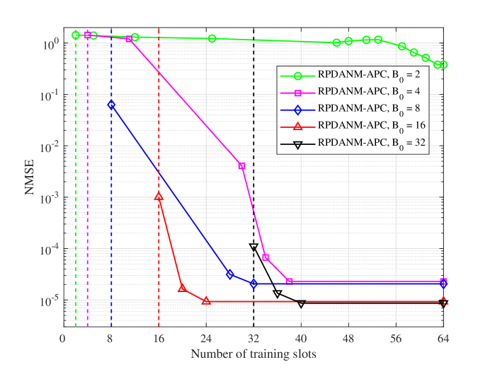
Figure 8: NMSE of RPDANM-APC versus the number of training slots with different $B_{0}$. Dashed lines indicate the initial number of training slots.

Furthermore, we investigate the effect of the initial number of training slots $B_{0}$ on the total number of training slots $B$ required for RPDANM-APC via Monte Carlo simulations. Fig. 9 illustrates the average number of required training slots under different $B_{0}$ versus the size of RIS. $N_{\mathrm{R}}$ increases from 16 to 128 and 100 Monte Carlo experiments are conducted under each setting. The black line denotes $B_{\max}$, i.e., the upper bound of number of training slots. It is observed that as $N_{\mathrm{R}}$ increases, the advantage of RPDANM-APC in saving training overhead is considerable. In particular, when $B_{0}$ is between 8 and 16, i.e., 2 to 4 times of the number of effective paths, the least training slots are required for convergence. On the one hand, when $B_{0}$ is small, e.g., $B_{0}=4$, imprecise initialization leads to more iterations required for convergence, resulting in more training overhead. On the other hand, when $B_{0}$ is large, e.g., $B_{0}=32$, too many initial training slots leads to a waste of training overhead. As a result, we recommend setting the initial number of training slots between $2\hat{L}$ and $4\hat{L}$, where $\hat{L}$ is the estimated number of effective paths.

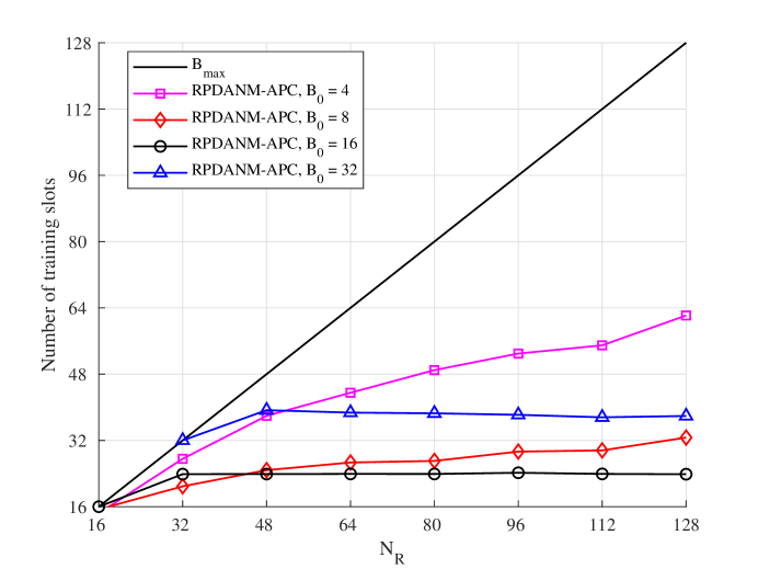
Figure 9: Average number of training slots of RPDANM-APC versus the size of RIS under different $B_{0}$.

VII Conclusions

In this paper, a PDANM-based CE framework was proposed for RIS-aided MIMO systems, which substantially reduces the computational complexity but only suffers a slight CE accuracy loss compared to state-of-the-art methods. A PDANM-based iterative algorithm called RPDANM was proposed next, which further promotes sparsity by approximately solving a rank minimization problem and thus achieves a higher CE accuracy than PDANM. Furthermore, by adaptively adjusting the RIS phases during CE, an iterative CE approach named RPDANM-APC was proposed, which strikes a balance between reduced training overhead and competitive CE performance. Numerical simulations were provided to demonstrate the high computational efficiency, superior CE accuracy, and excellent ability to save training overhead of our proposed methods, especially the RPDANM-APC approach. In future studies, we will extend PDANM to higher-dimensional cases and other parameter estimation scenarios. In addition, efficient algorithms will be developed to further reduce the computational cost of solving large-scale SDP problems.

Appendix A Proof of Proposition 1

For any $\kappa\in\mathbb{C}$ and $\xi\in[-\zeta,\zeta]$ where $\zeta=\min_{l_{\mathrm{BR}}\in\{1,\cdots,L_{\mathrm{BR}}\},l_{\mathrm{RU}}\in\{1,\cdots,L_{\mathrm{RU}}\}}\big{\{}1-\cos([\boldsymbol{\phi}^{\prime}_{\mathrm{R}}]_{l_{\mathrm{BR}}}),1+\cos([\boldsymbol{\phi}^{\prime}_{\mathrm{R}}]_{l_{\mathrm{BR}}}),1-\cos([\boldsymbol{\theta}^{\prime}_{\mathrm{R}}]_{l_{\mathrm{RU}}}),1+\cos([\boldsymbol{\theta}^{\prime}_{\mathrm{R}}]_{l_{\mathrm{RU}}})\big{\}}$, we take $\boldsymbol{\rho}^{\prime}_{\mathrm{BR}}=\kappa\boldsymbol{\rho}_{\mathrm{BR}}$ and $\boldsymbol{\rho}^{\prime}_{\mathrm{RU}}=\frac{1}{\kappa}\boldsymbol{\rho}_{\mathrm{RU}}$ and let $[\boldsymbol{\phi}^{\prime}_{\mathrm{R}}]_{l_{\mathrm{BR}}}=\arccos\big{(}\cos([\boldsymbol{\phi}_{\mathrm{R}}]_{l_{\mathrm{BR}}})+\xi\big{)}$ and $[\boldsymbol{\theta}^{\prime}_{\mathrm{R}}]_{l_{\mathrm{RU}}}=\arccos\big{(}\cos([\boldsymbol{\theta}_{\mathrm{R}}]_{l_{\mathrm{RU}}})+\xi\big{)}$, $\forall\ l_{\mathrm{BR}}\in\{1,\cdots,L_{\mathrm{BR}}\}$, $\forall\ l_{\mathrm{RU}}\in\{1,\cdots,L_{\mathrm{RU}}\}$. Then, we have

$$\big{[}\mathrm{diag}(\boldsymbol{\rho}^{\prime}_{\mathrm{RU}})\mathbf{A}^{H}_{N_{\mathrm{R}}}(\boldsymbol{\theta}^{\prime}_{\mathrm{R}})\cdot\mathrm{diag}(\boldsymbol{\omega}_{b})\cdot\mathbf{A}_{N_{\mathrm{R}}}(\boldsymbol{\phi}^{\prime}_{\mathrm{R}})\mathrm{diag}(\boldsymbol{\rho}^{\prime}_{\mathrm{BR}})\big{]}_{l_{\mathrm{RU}},l_{\mathrm{BR}}}$$ (31)

$$= [\boldsymbol{\rho}^{\prime}_{\mathrm{RU}}]_{l_{\mathrm{RU}}}[\boldsymbol{\rho}^{\prime}_{\mathrm{BR}}]_{l_{\mathrm{BR}}}\mathbf{a}^{H}_{N_{\mathrm{R}}}([\boldsymbol{\theta}^{\prime}_{\mathrm{R}}]_{l_{\mathrm{RU}}})\mathrm{diag}(\boldsymbol{\omega}_{b})\mathbf{a}_{N_{\mathrm{R}}}([\boldsymbol{\phi}^{\prime}_{\mathrm{R}}]_{l_{\mathrm{BR}}})$$

$$= [\boldsymbol{\rho}^{\prime}_{\mathrm{RU}}]_{l_{\mathrm{RU}}}[\boldsymbol{\rho}^{\prime}_{\mathrm{BR}}]_{l_{\mathrm{BR}}}\sum^{N_{\mathrm{R}}}_{n_{\mathrm{R}}=1}[\boldsymbol{\omega}_{b}]_{n_{\mathrm{R}}}\mathrm{e}^{-i\pi(n_{\mathrm{R}}-1)\cos([\boldsymbol{\theta}^{\prime}_{\mathrm{R}}]_{l_{\mathrm{RU}}})}\mathrm{e}^{i\pi(n_{\mathrm{R}}-1)\cos([\boldsymbol{\phi}^{\prime}_{\mathrm{R}}]_{l_{\mathrm{BR}}})}$$

$$= \frac{1}{\kappa}[\boldsymbol{\rho}_{\mathrm{RU}}]_{l_{\mathrm{RU}}}\cdot\kappa[\boldsymbol{\rho}_{\mathrm{BR}}]_{l_{\mathrm{BR}}}\cdot\sum^{N_{\mathrm{R}}}_{n_{\mathrm{R}}=1}[\boldsymbol{\omega}_{b}]_{n_{\mathrm{R}}}\mathrm{e}^{i\pi(n_{\mathrm{R}}-1)\big{[}\cos([\boldsymbol{\phi}_{\mathrm{R}}]_{l_{\mathrm{BR}}})+\xi-\cos([\boldsymbol{\theta}_{\mathrm{R}}]_{l_{\mathrm{RU}}})-\xi\big{]}}$$

$$= [\boldsymbol{\rho}_{\mathrm{RU}}]_{l_{\mathrm{RU}}}[\boldsymbol{\rho}_{\mathrm{BR}}]_{l_{\mathrm{BR}}}\sum^{N_{\mathrm{R}}}_{n_{\mathrm{R}}=1}[\boldsymbol{\omega}_{b}]_{n_{\mathrm{R}}}\mathrm{e}^{-i\pi(n_{\mathrm{R}}-1)\cos([\boldsymbol{\theta}_{\mathrm{R}}]_{l_{\mathrm{RU}}})}\mathrm{e}^{i\pi(n_{\mathrm{R}}-1)\cos([\boldsymbol{\phi}_{\mathrm{R}}]_{l_{\mathrm{BR}}})}$$

$$= \big{[}\mathrm{diag}(\boldsymbol{\rho}_{\mathrm{RU}})\mathbf{A}^{H}_{N_{\mathrm{R}}}(\boldsymbol{\theta}_{\mathrm{R}})\cdot\mathrm{diag}(\boldsymbol{\omega}_{b})\cdot\mathbf{A}_{N_{\mathrm{R}}}(\boldsymbol{\phi}_{\mathrm{R}})\mathrm{diag}(\boldsymbol{\rho}_{\mathrm{BR}})\big{]}_{l_{\mathrm{BR}},l_{\mathrm{RU}}}.$$

It follows that

$$\mathbf{H}^{b}_{\mathrm{BU}} =\mathbf{A}_{N_{\mathrm{U}}}(\boldsymbol{\phi}_{\mathrm{U}})\mathrm{diag}(\boldsymbol{\rho}_{\mathrm{RU}})\mathbf{A}^{H}_{N_{\mathrm{R}}}(\boldsymbol{\theta}_{\mathrm{R}})\cdot\mathrm{diag}(\boldsymbol{\omega}_{b})\cdot\mathbf{A}_{N_{\mathrm{R}}}(\boldsymbol{\phi}_{\mathrm{R}})\mathrm{diag}(\boldsymbol{\rho}_{\mathrm{BR}})\mathbf{A}^{H}_{N_{\mathrm{B}}}(\boldsymbol{\theta}_{\mathrm{B}})$$ (32)

$$=\mathbf{A}_{N_{\mathrm{U}}}(\boldsymbol{\phi}_{\mathrm{U}})\mathrm{diag}(\boldsymbol{\rho}^{\prime}_{\mathrm{RU}})\mathbf{A}^{H}_{N_{\mathrm{R}}}(\boldsymbol{\theta}^{\prime}_{\mathrm{R}})\cdot\mathrm{diag}(\boldsymbol{\omega}_{b})\cdot\mathbf{A}_{N_{\mathrm{R}}}(\boldsymbol{\phi}^{\prime}_{\mathrm{R}})\mathrm{diag}(\boldsymbol{\rho}^{\prime}_{\mathrm{BR}})\mathbf{A}^{H}_{N_{\mathrm{B}}}(\boldsymbol{\theta}_{\mathrm{B}}).$$

Appendix B Proof of Theorem 1

We first show that $\mathrm{SDP}(\mathbf{H})\leq\|\mathbf{H}\|_{\mathcal{A}}$. Assume that

$$\mathbf{H} =\sum_{l_{\mathrm{BU}}}\sum_{l_{\mathrm{R}}}[\mathbf{P}]_{l_{\mathrm{BU}},l_{\mathrm{R}}}\big{[}\mathbf{a}_{N_{\mathrm{B}}}([\boldsymbol{\theta}]_{l_{\mathrm{BU}}})\otimes\mathbf{a}_{N_{\mathrm{U}}}([\boldsymbol{\phi}]_{l_{\mathrm{BU}}})\big{]}\mathbf{a}^{H}_{N_{\mathrm{R}}}(\psi_{l_{\mathrm{R}}})$$ (33)

$$=\big{[}\mathbf{A}_{N_{\mathrm{B}}}(\boldsymbol{\theta})\diamond\mathbf{A}_{N_{\mathrm{U}}}(\boldsymbol{\phi})\big{]}\mathbf{P}\mathbf{A}^{H}_{N_{\mathrm{R}}}(\boldsymbol{\psi})$$

is a partially decoupled atomic decomposition of the effective channel, where $\mathbf{P}$ is not necessarily a diagonal matrix since there may be repeated entries in $\boldsymbol{\theta}$ and $\boldsymbol{\phi}$ since different partially decoupled atoms may overlap in some dimensions. We take

$$\mathcal{T}_{[N_{\mathrm{B}},N_{\mathrm{U}}]}(\mathbf{T}) =\sum_{l_{\mathrm{BU}}}\sum_{l_{\mathrm{R}}}\left|[\mathbf{P}]_{l_{\mathrm{BU}},l_{\mathrm{R}}}\right|\big{[}\mathbf{a}_{N_{\mathrm{B}}}([\boldsymbol{\theta}]_{l_{\mathrm{BU}}})\otimes\mathbf{a}_{N_{\mathrm{U}}}([\boldsymbol{\phi}]_{l_{\mathrm{BU}}})\big{]}\big{[}\mathbf{a}_{N_{\mathrm{B}}}([\boldsymbol{\theta}]_{l_{\mathrm{BU}}})\otimes\mathbf{a}_{N_{\mathrm{U}}}([\boldsymbol{\phi}]_{l_{\mathrm{BU}}})\big{]}^{H}$$ (34)

and

$$\mathcal{T}_{N_{\mathrm{R}}}(\mathbf{t})=\sum_{l_{\mathrm{BU}}}\sum_{l_{\mathrm{R}}}\left|[\mathbf{P}]_{l_{\mathrm{BU}},l_{\mathrm{R}}}\right|\mathbf{a}_{N_{\mathrm{R}}}(\psi_{l_{\mathrm{R}}})\mathbf{a}^{H}_{N_{\mathrm{R}}}(\psi_{l_{\mathrm{R}}}).$$ (35)

It follows that

$$\begin{bmatrix}\mathcal{T}_{N_{\mathrm{R}}}(\mathbf{t})&\mathbf{H}^{H}\\ \mathbf{H}&\mathcal{T}_{[N_{\mathrm{B}},N_{\mathrm{U}}]}(\mathbf{T})\end{bmatrix} =\sum_{l_{\mathrm{BU}}}\sum_{l_{\mathrm{R}}}\left|[\mathbf{P}]_{l_{\mathrm{BU}},l_{\mathrm{R}}}\right|$$ (36)

$$\quad\cdot\begin{bmatrix}\frac{\overline{[\mathbf{P}]_{l_{\mathrm{BU}},l_{\mathrm{R}}}}}{\left|[\mathbf{P}]_{l_{\mathrm{BU}},l_{\mathrm{R}}}\right|}\mathbf{a}_{N_{\mathrm{R}}}(\psi_{l_{\mathrm{R}}})\\ \mathbf{a}_{N_{\mathrm{B}}}([\boldsymbol{\theta}]_{l_{\mathrm{BU}}})\otimes\mathbf{a}_{N_{\mathrm{U}}}([\boldsymbol{\phi}]_{l_{\mathrm{BU}}})\end{bmatrix}\begin{bmatrix}\frac{\overline{[\mathbf{P}]_{l_{\mathrm{BU}},l_{\mathrm{R}}}}}{\left|[\mathbf{P}]_{l_{\mathrm{BU}},l_{\mathrm{R}}}\right|}\mathbf{a}_{N_{\mathrm{R}}}(\psi_{l_{\mathrm{R}}})\\ \mathbf{a}_{N_{\mathrm{B}}}([\boldsymbol{\theta}]_{l_{\mathrm{BU}}})\otimes\mathbf{a}_{N_{\mathrm{U}}}([\boldsymbol{\phi}]_{l_{\mathrm{BU}}})\end{bmatrix}^{H}\succeq\mathbf{0},$$

and thus

$$\mathrm{SDP}(\mathbf{H}) \leq\frac{1}{2N_{\mathrm{R}}}\mathrm{tr}\big{(}\mathcal{T}_{N_{\mathrm{R}}}(\mathbf{t})\big{)}+\frac{1}{2N_{\mathrm{B}}N_{\mathrm{U}}}\mathrm{tr}\big{(}\mathcal{T}_{[N_{\mathrm{B}},N_{\mathrm{U}}]}(\mathbf{T})\big{)}$$ (37)

$$=\frac{1}{2N_{\mathrm{R}}}\sum_{l_{\mathrm{BU}}}\sum_{l_{\mathrm{R}}}\left|[\mathbf{P}]_{l_{\mathrm{BU}},l_{\mathrm{R}}}\right|\mathbf{a}^{H}_{N_{\mathrm{R}}}(\psi_{l_{\mathrm{R}}})\mathbf{a}_{N_{\mathrm{R}}}(\psi_{l_{\mathrm{R}}})+\frac{1}{2N_{\mathrm{B}}N_{\mathrm{U}}}\sum_{l_{\mathrm{BU}}}\sum_{l_{\mathrm{R}}}\left|[\mathbf{P}]_{l_{\mathrm{BU}},l_{\mathrm{R}}}\right|$$

$$\quad\cdot\big{[}\mathbf{a}_{N_{\mathrm{B}}}([\boldsymbol{\theta}]_{l_{\mathrm{BU}}})\otimes\mathbf{a}_{N_{\mathrm{U}}}([\boldsymbol{\phi}]_{l_{\mathrm{BU}}})\big{]}^{H}\big{[}\mathbf{a}_{N_{\mathrm{B}}}([\boldsymbol{\theta}]_{l_{\mathrm{BU}}})\otimes\mathbf{a}_{N_{\mathrm{U}}}([\boldsymbol{\phi}]_{l_{\mathrm{BU}}})\big{]}$$

$$=\sum_{l_{\mathrm{BU}}}\sum_{l_{\mathrm{R}}}\left|[\mathbf{P}]_{l_{\mathrm{BU}},l_{\mathrm{R}}}\right|.$$

Since (37) holds for any partially decoupled atomic decomposition of $\mathbf{H}$, we have that $\mathrm{SDP}(\mathbf{H})\leq\|\mathbf{H}\|_{\mathcal{A}}$.

We next show that $\mathrm{SDP}(\mathbf{H})=\|\mathbf{H}\|_{\mathcal{A}}$ under the three conditions in Theorem 1. Due to the column inclusion property [36] of PSD matrices, we have that $\mathrm{col}\big{(}\mathbf{H}^{H}\big{)}\in\mathrm{col}\big{(}\mathcal{T}_{N_{\mathrm{R}}}(\mathbf{t}^{*})\big{)}$ and $\mathrm{col}\big{(}\mathbf{H}\big{)}\in\mathrm{col}\big{(}\mathcal{T}_{[N_{\mathrm{B}},N_{\mathrm{U}}]}(\mathbf{T}^{*})\big{)}$. It follows from (18) and (19) that there exists a matrix $\mathbf{C}\in\mathbb{C}^{L_{\mathrm{BU}}^{*}\times L_{\mathrm{R}}^{*}}$ such that $\mathbf{H}$ admits the following partially decoupled atomic decomposition:

$$\mathbf{H}=\big{[}\mathbf{A}_{N_{\mathrm{B}}}(\boldsymbol{\theta}_{\mathrm{B}}^{*})\diamond\mathbf{A}_{N_{\mathrm{U}}}(\boldsymbol{\phi}_{\mathrm{U}}^{*})\big{]}\mathbf{C}\mathbf{A}^{H}_{N_{\mathrm{R}}}(\boldsymbol{\psi}_{\mathrm{R}}^{*}).$$ (38)

We first assume that there is exactly one non-zero element in each row of $\mathbf{C}$, denoted as $[\mathbf{C}]_{i,k_{i}}$ in the $i$-th row. It follows from the Schur complement theorem [37] that $\mathcal{T}_{N_{\mathrm{R}}}(\mathbf{t}^{*})\succeq\mathbf{H}^{H}{\mathcal{T}_{[N_{\mathrm{B}},N_{\mathrm{U}}]}(\mathbf{T}^{*})}^{\dagger}\mathbf{H}$, i.e.,

$$\mathbf{A}_{N_{\mathrm{R}}}(\boldsymbol{\psi}_{\mathrm{R}}^{*})\mathrm{diag}(\mathbf{p}_{\mathrm{R}}^{*})\mathbf{A}^{H}_{N_{\mathrm{B}}}(\boldsymbol{\psi}_{\mathrm{R}}^{*})$$ (39)

$$\succeq \mathbf{A}_{N_{\mathrm{R}}}(\boldsymbol{\psi}_{\mathrm{R}}^{*})\mathbf{C}^{H}\big{[}\mathbf{A}_{N_{\mathrm{B}}}(\boldsymbol{\theta}_{\mathrm{B}}^{*})\diamond\mathbf{A}_{N_{\mathrm{U}}}(\boldsymbol{\phi}_{\mathrm{U}}^{*})\big{]}^{H}{\big{[}\mathbf{A}_{N_{\mathrm{B}}}(\boldsymbol{\theta}_{\mathrm{B}}^{*})\diamond\mathbf{A}_{N_{\mathrm{U}}}(\boldsymbol{\phi}_{\mathrm{U}}^{*})\big{]}^{H}}^{\dagger}$$

$$\cdot{\mathrm{diag}(\mathbf{p}_{\mathrm{BU}}^{*})}^{\dagger}\big{[}\mathbf{A}_{N_{\mathrm{B}}}(\boldsymbol{\theta}_{\mathrm{B}}^{*})\diamond\mathbf{A}_{N_{\mathrm{U}}}(\boldsymbol{\phi}_{\mathrm{U}}^{*})\big{]}^{\dagger}\big{[}\mathbf{A}_{N_{\mathrm{B}}}(\boldsymbol{\theta}_{\mathrm{B}}^{*})\diamond\mathbf{A}_{N_{\mathrm{U}}}(\boldsymbol{\phi}_{\mathrm{U}}^{*})\big{]}\mathbf{C}\mathbf{A}^{H}_{N_{\mathrm{R}}}(\boldsymbol{\psi}_{\mathrm{R}}^{*})$$

$$= \mathbf{A}_{N_{\mathrm{R}}}(\boldsymbol{\psi}_{\mathrm{R}}^{*})\mathbf{C}^{H}{\mathrm{diag}(\mathbf{p}_{\mathrm{BU}}^{*})}^{\dagger}\mathbf{C}\mathbf{A}^{H}_{N_{\mathrm{R}}}(\boldsymbol{\psi}_{\mathrm{R}}^{*}).$$

From (39), we obtain

$$\mathrm{diag}(\mathbf{p}_{\mathrm{R}}^{*})\succeq\mathbf{C}^{H}{\mathrm{diag}(\mathbf{p}_{\mathrm{BU}}^{*})}^{\dagger}\mathbf{C},$$ (40)

which yields

$$[\mathbf{p}_{\mathrm{R}}^{*}]_{l_{\mathrm{R}}}\geq\sum_{l_{\mathrm{BU}}=1}^{L_{\mathrm{BU}}^{*}}\frac{\left|[\mathbf{C}]_{l_{\mathrm{BU}},l_{\mathrm{R}}}\right|^{2}}{[\mathbf{p}_{\mathrm{BU}}^{*}]_{l_{\mathrm{BU}}}},l_{\mathrm{R}}=1,\cdots,L_{\mathrm{R}}^{*}$$ (41)

since $\mathbf{C}^{H}{\mathrm{diag}(\mathbf{p}_{\mathrm{BU}}^{*})}^{\dagger}\mathbf{C}$ is a diagonal matrix. Then, we have

$$\mathrm{SDP}(\mathbf{H}) =\frac{1}{2N_{\mathrm{R}}}\mathrm{tr}\big{(}\mathcal{T}_{N_{\mathrm{R}}}(\mathbf{t}^{*})\big{)}+\frac{1}{2N_{\mathrm{B}}N_{\mathrm{U}}}\mathrm{tr}\big{(}\mathcal{T}_{[N_{\mathrm{B}},N_{\mathrm{U}}]}(\mathbf{T}^{*})\big{)}$$ (42)

$$=\frac{1}{2N_{\mathrm{R}}}\sum_{l_{\mathrm{R}}=1}^{L_{\mathrm{R}}^{*}}[\mathbf{p}_{\mathrm{R}}^{*}]_{l_{\mathrm{R}}}\mathbf{a}^{H}_{N_{\mathrm{R}}}([\boldsymbol{\psi}_{\mathrm{R}}^{*}]_{l_{R}})\mathbf{a}_{N_{\mathrm{R}}}([\boldsymbol{\psi}_{\mathrm{R}}^{*}]_{l_{R}})+\frac{1}{2N_{\mathrm{B}}N_{\mathrm{U}}}\sum_{l_{\mathrm{BU}}=1}^{L_{\mathrm{BU}}^{*}}[\mathbf{p}_{\mathrm{BU}}^{*}]_{l_{\mathrm{BU}}}$$

$$\quad\cdot\big{[}\mathbf{a}_{N_{\mathrm{B}}}([\boldsymbol{\theta}_{\mathrm{B}}^{*}]_{l_{BU}})\otimes\mathbf{a}_{N_{\mathrm{U}}}([\boldsymbol{\phi}_{\mathrm{U}}^{*}]_{l_{BU}})\big{]}^{H}\big{[}\mathbf{a}_{N_{\mathrm{B}}}([\boldsymbol{\theta}_{\mathrm{B}}^{*}]_{l_{BU}})\otimes\mathbf{a}_{N_{\mathrm{U}}}([\boldsymbol{\phi}_{\mathrm{U}}^{*}]_{l_{BU}})\big{]}$$

$$=\frac{1}{2}\sum_{l_{\mathrm{R}}=1}^{L_{\mathrm{R}}^{*}}[\mathbf{p}_{\mathrm{R}}^{*}]_{l_{\mathrm{R}}}+\frac{1}{2}\sum_{l_{\mathrm{BU}}=1}^{L_{\mathrm{BU}}^{*}}[\mathbf{p}_{\mathrm{BU}}^{*}]_{l_{\mathrm{BU}}}$$

$$\geq\frac{1}{2}\sum_{l_{\mathrm{R}}=1}^{L_{\mathrm{R}}^{*}}\sum_{l_{\mathrm{BU}}=1}^{L_{\mathrm{BU}}^{*}}\frac{\left|[\mathbf{C}]_{l_{\mathrm{BU}},l_{\mathrm{R}}}\right|^{2}}{[\mathbf{p}_{\mathrm{BU}}^{*}]_{l_{\mathrm{BU}}}}+\frac{1}{2}\sum_{l_{\mathrm{BU}}=1}^{L_{\mathrm{BU}}^{*}}[\mathbf{p}_{\mathrm{BU}}^{*}]_{l_{\mathrm{BU}}}$$

$$=\frac{1}{2}\sum_{l_{\mathrm{BU}}=1}^{L_{\mathrm{BU}}^{*}}\frac{\left|[\mathbf{C}]_{l_{\mathrm{BU}},k_{l_{\mathrm{BU}}}}\right|^{2}}{[\mathbf{p}_{\mathrm{BU}}^{*}]_{l_{\mathrm{BU}}}}+\frac{1}{2}\sum_{l_{\mathrm{BU}}=1}^{L_{\mathrm{BU}}^{*}}[\mathbf{p}_{\mathrm{BU}}^{*}]_{l_{\mathrm{BU}}}$$

$$\geq\sum_{l_{\mathrm{BU}}=1}^{L_{\mathrm{BU}}^{*}}\left|[\mathbf{C}]_{l_{\mathrm{BU}},k_{l_{\mathrm{BU}}}}\right|\geq\|\mathbf{H}\|_{\mathcal{A}}.$$

Combining (42) and (37), we draw the conclusion that $\mathrm{SDP}(\mathbf{H})=\|\mathbf{H}\|_{\mathcal{A}}$.

Similarly, if there is exactly one non-zero element in each column of $\mathbf{C}$, denoted as $[\mathbf{C}]_{k_{j},j}$ in the $j$-th column, it follows that $\mathcal{T}_{[N_{\mathrm{B}},N_{\mathrm{U}}]}(\mathbf{T}^{*})\succeq\mathbf{H}{\mathcal{T}_{N_{\mathrm{R}}}(\mathbf{t}^{*})}^{\dagger}\mathbf{H}^{H}$. Similarly to the derivations above, we obtain that

$$\mathrm{diag}(\mathbf{p}_{\mathrm{BU}}^{*})\succeq\mathbf{C}{\mathrm{diag}(\mathbf{p}_{\mathrm{R}}^{*})}^{\dagger}\mathbf{C}^{H},$$ (43)

or equivalently,

$$[\mathbf{p}_{\mathrm{BU}}^{*}]_{l_{\mathrm{BU}}}\geq\sum_{l_{\mathrm{R}}=1}^{L_{\mathrm{R}}^{*}}\frac{\left|[\mathbf{C}]_{l_{\mathrm{BU}},l_{\mathrm{R}}}\right|^{2}}{[\mathbf{p}_{\mathrm{R}}^{*}]_{l_{\mathrm{R}}}},l_{\mathrm{BU}}=1,\cdots,L_{\mathrm{BU}}^{*},$$ (44)

since $\mathbf{C}{\mathrm{diag}(\mathbf{p}_{\mathrm{R}}^{*})}^{\dagger}\mathbf{C}^{H}$ is a diagonal matrix. Then, we have

$$\mathrm{SDP}(\mathbf{H}) =\frac{1}{2}\sum_{l_{\mathrm{R}}=1}^{L_{\mathrm{R}}^{*}}[\mathbf{p}_{\mathrm{R}}^{*}]_{l_{\mathrm{R}}}+\frac{1}{2}\sum_{l_{\mathrm{BU}}=1}^{L_{\mathrm{BU}}^{*}}[\mathbf{p}_{\mathrm{BU}}^{*}]_{l_{\mathrm{BU}}}$$ (45)

$$\geq\frac{1}{2}\sum_{l_{\mathrm{R}}=1}^{L_{\mathrm{R}}^{*}}[\mathbf{p}_{\mathrm{R}}^{*}]_{l_{\mathrm{R}}}+\frac{1}{2}\sum_{l_{\mathrm{BU}}=1}^{L_{\mathrm{BU}}^{*}}\sum_{l_{\mathrm{R}}=1}^{L_{\mathrm{R}}^{*}}\frac{\left|[\mathbf{C}]_{l_{\mathrm{BU}},l_{\mathrm{R}}}\right|^{2}}{[\mathbf{p}_{\mathrm{R}}^{*}]_{l_{\mathrm{R}}}}$$

$$=\frac{1}{2}\sum_{l_{\mathrm{R}}=1}^{L_{\mathrm{R}}^{*}}[\mathbf{p}_{\mathrm{R}}^{*}]_{l_{\mathrm{R}}}+\frac{1}{2}\sum_{l_{\mathrm{R}}=1}^{L_{\mathrm{R}}^{*}}\frac{\left|[\mathbf{C}]_{k_{l_{\mathrm{R}}},l_{\mathrm{R}}}\right|^{2}}{[\mathbf{p}_{\mathrm{R}}^{*}]_{l_{\mathrm{R}}}}$$

$$\geq\sum_{l_{\mathrm{R}}=1}^{L_{\mathrm{R}}^{*}}\left|[\mathbf{C}]_{k_{l_{\mathrm{R}}},l_{\mathrm{R}}}\right|\geq\|\mathbf{H}\|_{\mathcal{A}}.$$

Combining (45) and (37), we obtain that $\mathrm{SDP}(\mathbf{H})=\|\mathbf{H}\|_{\mathcal{A}}$ and complete the proof.

Appendix C Proof of Theorem 2

It follows from the proof of Theorem 1 that $\mathrm{SDP}(\mathbf{H})\leq\|\mathbf{H}\|_{\mathcal{A}}$ holds. Next, we will show that $\mathrm{SDP}(\mathbf{H})\geq\|\mathbf{H}\|_{\mathcal{A}}$. Define the one-dimensional (1D) atomic set as

$$\mathcal{A}_{1D} =\Big{\{}\mathbf{b}\mathbf{a}^{H}_{N_{\mathrm{R}}}(\psi)\in\mathbb{C}^{N_{\mathrm{B}}N_{\mathrm{U}}\times N_{\mathrm{R}}}:\psi\in[0,\pi],\|\mathbf{b}\|_{2}=1\Big{\}}$$ (46)

and the corresponding 1D atomic norm as

$$\|\mathbf{H}\|_{\mathcal{A}_{1D}} =\inf\Big{\{}\sum_{l}|\rho_{l}|:\mathbf{H}=\sum_{l}\rho_{l}\mathbf{b}_{l}\mathbf{a}^{H}_{N_{\mathrm{R}}}(\psi_{l}):\psi_{l}\in[0,\pi],\|\mathbf{b}_{l}\|_{2}=1\Big{\}},$$ (47)

then the effective channel $\mathbf{H}$ admits a 1D atomic decomposition in the 1D atomic set as

$$\mathbf{H}=\sum_{l_{\mathrm{BR}}=1}^{L_{\mathrm{BR}}}\sum_{l_{\mathrm{RU}}=1}^{L_{\mathrm{RU}}}\sqrt{N_{\mathrm{B}}N_{\mathrm{U}}}[\boldsymbol{\rho}_{\mathrm{BU}}]_{l_{\mathrm{BU}}}\big{[}\frac{1}{\sqrt{N_{\mathrm{B}}N_{\mathrm{U}}}}\mathbf{a}_{N_{\mathrm{B}}}([-\boldsymbol{\theta}_{\mathrm{B}}]_{l_{\mathrm{BR}}})\otimes\mathbf{a}_{N_{\mathrm{U}}}([\boldsymbol{\phi}_{\mathrm{U}}]_{l_{\mathrm{RU}}})\big{]}\mathbf{a}^{H}_{N_{\mathrm{R}}}([\boldsymbol{\psi}_{\mathrm{R}}]_{l_{\mathrm{BU}}}).$$ (48)

Denote $\mathrm{SDP}_{1D}(\mathbf{H})$ as the optimal value of the following SDP problem:

$$\min_{\mathbf{t},\mathbf{Q}}\frac{1}{2N_{\mathrm{R}}}\mathrm{tr}\big{(}\mathcal{T}_{N_{\mathrm{R}}}(\mathbf{t})\big{)}+\frac{1}{2N_{\mathrm{B}}N_{\mathrm{U}}}\mathrm{tr}\big{(}\mathbf{Q}\big{)},\ \mathrm{s.t.}\begin{bmatrix}\mathcal{T}_{N_{\mathrm{R}}}(\mathbf{t})&\mathbf{H}^{H}\\ \mathbf{H}&\mathbf{Q}\end{bmatrix}\succeq\mathbf{0}.$$ (49)

It is noted that (17) essentially imposes an additional constraint that $\mathbf{Q}$ is a 2-level Toeplitz matrix on (49) and thus

$$\mathrm{SDP}(\mathbf{H})\geq\mathrm{SDP}_{1D}(\mathbf{H}).$$ (50)

It follows from [29, Theorem 3] that

$$\mathrm{SDP}_{1D}(\mathbf{H})=\frac{1}{\sqrt{N_{\mathrm{B}}N_{\mathrm{U}}}}\|\mathbf{H}\|_{\mathcal{A}_{1D}}.$$ (51)

Since $\Delta_{\boldsymbol{\psi}_{\mathrm{R}}}>\frac{4}{N_{\mathrm{R}}}$, it is proved in [29, Theorem 4] that

$$\frac{1}{\sqrt{N_{\mathrm{B}}N_{\mathrm{U}}}}\|\mathbf{H}\|_{\mathcal{A}_{1D}}=\sum_{l_{\mathrm{BR}}=1}^{L_{\mathrm{BR}}}\sum_{l_{\mathrm{RU}}=1}^{L_{\mathrm{RU}}}|[\boldsymbol{\rho}_{\mathrm{BU}}]_{l_{\mathrm{BU}}}|$$ (52)

with $l_{\mathrm{BU}}=(l_{\mathrm{BR}}-1)L_{\mathrm{RU}}+l_{\mathrm{RU}}$. Furthermore, we have that

$$\sum_{l_{\mathrm{BR}}=1}^{L_{\mathrm{BR}}}\sum_{l_{\mathrm{RU}}=1}^{L_{\mathrm{RU}}}|[\boldsymbol{\rho}_{\mathrm{BU}}]_{l_{\mathrm{BU}}}|\geq\|\mathbf{H}\|_{\mathcal{A}},$$ (53)

since (10) is a partially decoupled atomic decomposition of $\mathbf{H}$. Combining (50), (51), (52), and (53), we have

$$\mathrm{SDP}(\mathbf{H})\geq\mathrm{SDP}_{1D}(\mathbf{H})=\frac{1}{\sqrt{N_{\mathrm{B}}N_{\mathrm{U}}}}\|\mathbf{H}\|_{\mathcal{A}_{1D}}=\sum_{l_{\mathrm{BR}}=1}^{L_{\mathrm{BR}}}\sum_{l_{\mathrm{RU}}=1}^{L_{\mathrm{RU}}}|[\boldsymbol{\rho}_{\mathrm{BU}}]_{l_{\mathrm{BU}}}|\geq\|\mathbf{H}\|_{\mathcal{A}}$$ (54)

and complete the proof.

Appendix D Proof of Theorem 3

The proof is a generalization of that of Theorem 1. We first show that $\mathrm{SDP}_{\mathbf{W}_{\mathrm{R}},\mathbf{W}_{\mathrm{BU}}}(\mathbf{H})\leq\|\mathbf{H}\|_{\mathcal{A}^{w_{\mathrm{R}},w_{\mathrm{BU}}}}$. For any partially decoupled atomic decomposition of $\mathbf{H}$ as in (33), we take

$$\mathcal{T}_{[N_{\mathrm{B}},N_{\mathrm{U}}]}(\mathbf{T}) =\sum_{l_{\mathrm{BU}}}\sum_{l_{\mathrm{R}}}\frac{w_{\mathrm{BU}}([\boldsymbol{\theta}]_{l_{\mathrm{BU}}},[\boldsymbol{\phi}]_{l_{\mathrm{BU}}})^{\frac{1}{2}}}{w_{\mathrm{R}}(\psi_{l_{\mathrm{R}}})^{\frac{1}{2}}}\left|[\mathbf{P}]_{l_{\mathrm{BU}},l_{\mathrm{R}}}\right|$$ (55)

$$\quad\cdot\big{[}\mathbf{a}_{N_{\mathrm{B}}}([\boldsymbol{\theta}]_{l_{\mathrm{BU}}})\otimes\mathbf{a}_{N_{\mathrm{U}}}([\boldsymbol{\phi}]_{l_{\mathrm{BU}}})\big{]}\big{[}\mathbf{a}_{N_{\mathrm{B}}}([\boldsymbol{\theta}]_{l_{\mathrm{BU}}})\otimes\mathbf{a}_{N_{\mathrm{U}}}([\boldsymbol{\phi}]_{l_{\mathrm{BU}}})\big{]}^{H}$$

and

$$\mathcal{T}_{N_{\mathrm{R}}}(\mathbf{t})=\sum_{l_{\mathrm{BU}}}\sum_{l_{\mathrm{R}}}\frac{w_{\mathrm{R}}(\psi_{l_{\mathrm{R}}})^{\frac{1}{2}}}{w_{\mathrm{BU}}([\boldsymbol{\theta}]_{l_{\mathrm{BU}}},[\boldsymbol{\phi}]_{l_{\mathrm{BU}}})^{\frac{1}{2}}}\left|[\mathbf{P}]_{l_{\mathrm{BU}},l_{\mathrm{R}}}\right|\mathbf{a}_{N_{\mathrm{R}}}(\psi_{l_{\mathrm{R}}})\mathbf{a}^{H}_{N_{\mathrm{R}}}(\psi_{l_{\mathrm{R}}}).$$ (56)

It follows that

$$\begin{bmatrix}\mathcal{T}_{N_{\mathrm{R}}}(\mathbf{t})&\mathbf{H}^{H}\\ \mathbf{H}&\mathcal{T}_{[N_{\mathrm{B}},N_{\mathrm{U}}]}(\mathbf{T})\end{bmatrix} =\sum_{l_{\mathrm{BU}}}\sum_{l_{\mathrm{R}}}\left|[\mathbf{P}]_{l_{\mathrm{BU}},l_{\mathrm{R}}}\right|\begin{bmatrix}\frac{\overline{[\mathbf{P}]_{l_{\mathrm{BU}},l_{\mathrm{R}}}}}{\left|[\mathbf{P}]_{l_{\mathrm{BU}},l_{\mathrm{R}}}\right|}\frac{w_{\mathrm{R}}(\psi_{l_{\mathrm{R}}})^{\frac{1}{4}}}{w_{\mathrm{BU}}([\boldsymbol{\theta}]_{l_{\mathrm{BU}}},[\boldsymbol{\phi}]_{l_{\mathrm{BU}}})^{\frac{1}{4}}}\mathbf{a}_{N_{\mathrm{R}}}(\psi_{l_{\mathrm{R}}})\\ \frac{w_{\mathrm{BU}}([\boldsymbol{\theta}]_{l_{\mathrm{BU}}},[\boldsymbol{\phi}]_{l_{\mathrm{BU}}})^{\frac{1}{4}}}{w_{\mathrm{R}}(\psi_{l_{\mathrm{R}}})^{\frac{1}{4}}}\mathbf{a}_{N_{\mathrm{B}}}([\boldsymbol{\theta}]_{l_{\mathrm{BU}}})\otimes\mathbf{a}_{N_{\mathrm{U}}}([\boldsymbol{\phi}]_{l_{\mathrm{BU}}})\end{bmatrix}$$ (57)

$$\quad\cdot\begin{bmatrix}\frac{\overline{[\mathbf{P}]_{l_{\mathrm{BU}},l_{\mathrm{R}}}}}{\left|[\mathbf{P}]_{l_{\mathrm{BU}},l_{\mathrm{R}}}\right|}\frac{w_{\mathrm{R}}(\psi_{l_{\mathrm{R}}})^{\frac{1}{4}}}{w_{\mathrm{BU}}([\boldsymbol{\theta}]_{l_{\mathrm{BU}}},[\boldsymbol{\phi}]_{l_{\mathrm{BU}}})^{\frac{1}{4}}}\mathbf{a}_{N_{\mathrm{R}}}(\psi_{l_{\mathrm{R}}})\\ \frac{w_{\mathrm{BU}}([\boldsymbol{\theta}]_{l_{\mathrm{BU}}},[\boldsymbol{\phi}]_{l_{\mathrm{BU}}})^{\frac{1}{4}}}{w_{\mathrm{R}}(\psi_{l_{\mathrm{R}}})^{\frac{1}{4}}}\mathbf{a}_{N_{\mathrm{B}}}([\boldsymbol{\theta}]_{l_{\mathrm{BU}}})\otimes\mathbf{a}_{N_{\mathrm{U}}}([\boldsymbol{\phi}]_{l_{\mathrm{BU}}})\end{bmatrix}^{H}\succeq\mathbf{0},$$

thus we have

$$\mathrm{SDP}_{\mathbf{W}_{\mathrm{R}},\mathbf{W}_{\mathrm{BU}}}(\mathbf{H}) \leq\frac{1}{2}\mathrm{tr}\big{(}\mathbf{W}_{\mathrm{R}}\mathcal{T}_{N_{\mathrm{R}}}(\mathbf{t})\big{)}+\frac{1}{2}\mathrm{tr}\big{(}\mathbf{W}_{\mathrm{BU}}\mathcal{T}_{[N_{\mathrm{B}},N_{\mathrm{U}}]}(\mathbf{T})\big{)}$$ (58)

$$=\frac{1}{2}\sum_{l_{\mathrm{BU}}}\sum_{l_{\mathrm{R}}}\left|[\mathbf{P}]_{l_{\mathrm{BU}},l_{\mathrm{R}}}\right|\frac{w_{\mathrm{R}}(\psi_{l_{\mathrm{R}}})^{\frac{1}{2}}}{w_{\mathrm{BU}}([\boldsymbol{\theta}]_{l_{\mathrm{BU}}},[\boldsymbol{\phi}]_{l_{\mathrm{BU}}})^{\frac{1}{2}}}\mathbf{a}^{H}_{N_{\mathrm{R}}}(\psi_{l_{\mathrm{R}}})\mathbf{W}_{\mathrm{R}}\mathbf{a}_{N_{\mathrm{R}}}(\psi_{l_{\mathrm{R}}})$$

$$\quad+\frac{1}{2}\sum_{l_{\mathrm{BU}}}\sum_{l_{\mathrm{R}}}\left|[\mathbf{P}]_{l_{\mathrm{BU}},l_{\mathrm{R}}}\right|\frac{w_{\mathrm{BU}}([\boldsymbol{\theta}]_{l_{\mathrm{BU}}},[\boldsymbol{\phi}]_{l_{\mathrm{BU}}})^{\frac{1}{2}}}{w_{\mathrm{R}}(\psi_{l_{\mathrm{R}}})^{\frac{1}{2}}}$$

$$\qquad\cdot\big{[}\mathbf{a}_{N_{\mathrm{B}}}([\boldsymbol{\theta}]_{l_{\mathrm{BU}}})\otimes\mathbf{a}_{N_{\mathrm{U}}}([\boldsymbol{\phi}]_{l_{\mathrm{BU}}})\big{]}^{H}\mathbf{W}_{\mathrm{BU}}\big{[}\mathbf{a}_{N_{\mathrm{B}}}([\boldsymbol{\theta}]_{l_{\mathrm{BU}}})\otimes\mathbf{a}_{N_{\mathrm{U}}}([\boldsymbol{\phi}]_{l_{\mathrm{BU}}})\big{]}$$

$$=\sum_{l_{\mathrm{BU}}}\sum_{l_{\mathrm{R}}}\left|[\mathbf{P}]_{l_{\mathrm{BU}},l_{\mathrm{R}}}\right|w_{\mathrm{BU}}([\boldsymbol{\theta}]_{l_{\mathrm{BU}}},[\boldsymbol{\phi}]_{l_{\mathrm{BU}}})^{-\frac{1}{2}}w_{\mathrm{R}}(\psi_{l_{\mathrm{R}}})^{-\frac{1}{2}}.$$

Since (58) holds for any partially decoupled atomic decomposition of $\mathbf{H}$, we have that $\mathrm{SDP}_{\mathbf{W}_{\mathrm{R}},\mathbf{W}_{\mathrm{BU}}}(\mathbf{H})\leq\|\mathbf{H}\|_{\mathcal{A}^{w_{\mathrm{R}},w_{\mathrm{BU}}}}$.

We next show that $\mathrm{SDP}_{\mathbf{W}_{\mathrm{R}},\mathbf{W}_{\mathrm{BU}}}(\mathbf{H})=\|\mathbf{H}\|_{\mathcal{A}^{w_{\mathrm{R}},w_{\mathrm{BU}}}}$ under the three conditions in Theorem 1. Without loss of generality, we assume that there is exactly one non-zero element in each row of $\mathbf{C}$, denoted as $[\mathbf{C}]_{i,k_{i}}$ in the $i$-th row. By derivations similar to those of Theorem 1, we obtain that (38), (40) and (41) hold. Then, it follows that

$$\mathrm{SDP}_{\mathbf{W}_{\mathrm{R}},\mathbf{W}_{\mathrm{BU}}}(\mathbf{H}) =\frac{1}{2}\mathrm{tr}\big{(}\mathbf{W}_{\mathrm{R}}\mathcal{T}_{N_{\mathrm{R}}}(\mathbf{t}^{*})\big{)}+\frac{1}{2}\mathrm{tr}\big{(}\mathbf{W}_{\mathrm{BU}}\mathcal{T}_{[N_{\mathrm{B}},N_{\mathrm{U}}]}(\mathbf{T}^{*})\big{)}$$ (59)

$$=\frac{1}{2}\sum_{l_{\mathrm{R}}=1}^{L_{\mathrm{R}}^{*}}[\mathbf{p}_{\mathrm{R}}^{*}]_{l_{\mathrm{R}}}\mathbf{a}^{H}_{N_{\mathrm{R}}}([\boldsymbol{\psi}_{\mathrm{R}}^{*}]_{l_{R}})\mathbf{W}_{\mathrm{R}}\mathbf{a}_{N_{\mathrm{R}}}([\boldsymbol{\psi}_{\mathrm{R}}^{*}]_{l_{R}})+\frac{1}{2}\sum_{l_{\mathrm{BU}}=1}^{L_{\mathrm{BU}}^{*}}[\mathbf{p}_{\mathrm{BU}}^{*}]_{l_{\mathrm{BU}}}$$

$$\quad\cdot\big{[}\mathbf{a}_{N_{\mathrm{B}}}([\boldsymbol{\theta}_{\mathrm{B}}^{*}]_{l_{BU}})\otimes\mathbf{a}_{N_{\mathrm{U}}}([\boldsymbol{\phi}_{\mathrm{U}}^{*}]_{l_{BU}})\big{]}^{H}\mathbf{W}_{\mathrm{BU}}\big{[}\mathbf{a}_{N_{\mathrm{B}}}([\boldsymbol{\theta}_{\mathrm{B}}^{*}]_{l_{BU}})\otimes\mathbf{a}_{N_{\mathrm{U}}}([\boldsymbol{\phi}_{\mathrm{U}}^{*}]_{l_{BU}})\big{]}$$

$$=\frac{1}{2}\sum_{l_{\mathrm{R}}=1}^{L_{\mathrm{R}}^{*}}w_{\mathrm{R}}([\boldsymbol{\psi}_{\mathrm{R}}^{*}]_{l_{R}})^{-1}[\mathbf{p}_{\mathrm{R}}^{*}]_{l_{\mathrm{R}}}+\frac{1}{2}\sum_{l_{\mathrm{BU}}=1}^{L_{\mathrm{BU}}^{*}}w_{\mathrm{BU}}([\boldsymbol{\theta}_{\mathrm{B}}^{*}]_{l_{BU}},[\boldsymbol{\phi}_{\mathrm{U}}^{*}]_{l_{BU}})^{-1}[\mathbf{p}_{\mathrm{BU}}^{*}]_{l_{\mathrm{BU}}}$$

$$\geq\frac{1}{2}\sum_{l_{\mathrm{R}}=1}^{L_{\mathrm{R}}^{*}}\sum_{l_{\mathrm{BU}}=1}^{L_{\mathrm{BU}}^{*}}w_{\mathrm{R}}([\boldsymbol{\psi}_{\mathrm{R}}^{*}]_{l_{R}})^{-1}\frac{\left|[\mathbf{C}]_{l_{\mathrm{BU}},l_{\mathrm{R}}}\right|^{2}}{[\mathbf{p}_{\mathrm{BU}}^{*}]_{l_{\mathrm{BU}}}}+\frac{1}{2}\sum_{l_{\mathrm{BU}}=1}^{L_{\mathrm{BU}}^{*}}w_{\mathrm{BU}}([\boldsymbol{\theta}_{\mathrm{B}}^{*}]_{l_{BU}},[\boldsymbol{\phi}_{\mathrm{U}}^{*}]_{l_{BU}})^{-1}[\mathbf{p}_{\mathrm{BU}}^{*}]_{l_{\mathrm{BU}}}$$

$$\geq\sum_{l_{\mathrm{BU}}=1}^{L_{\mathrm{BU}}^{*}}w_{\mathrm{R}}([\boldsymbol{\psi}_{\mathrm{R}}^{*}]_{k_{l_{\mathrm{BU}}}})^{-\frac{1}{2}}w_{\mathrm{BU}}([\boldsymbol{\theta}_{\mathrm{B}}^{*}]_{l_{BU}},[\boldsymbol{\phi}_{\mathrm{U}}^{*}]_{l_{BU}})^{-\frac{1}{2}}\left|[\mathbf{C}]_{l_{\mathrm{BU}},k_{l_{\mathrm{BU}}}}\right|\geq\|\mathbf{H}\|_{\mathcal{A}^{w_{\mathrm{R}},w_{\mathrm{BU}}}}.$$

Combining (59) and (58), we obtain that $\mathrm{SDP}(\mathbf{H})=\|\mathbf{H}\|_{\mathcal{A}^{w_{\mathrm{R}},w_{\mathrm{BU}}}}$. Similarly, if there is exactly one non-zero element in each column of $\mathbf{C}$, denoted as $[\mathbf{C}]_{k_{j},j}$ in the $j$-th column, we have (38), (43) and (44). It follows that

$$\mathrm{SDP}_{\mathbf{W}_{\mathrm{R}},\mathbf{W}_{\mathrm{BU}}}(\mathbf{H})= \frac{1}{2}\sum_{l_{\mathrm{R}}=1}^{L_{\mathrm{R}}^{*}}w_{\mathrm{R}}([\boldsymbol{\psi}_{\mathrm{R}}^{*}]_{l_{R}})^{-1}[\mathbf{p}_{\mathrm{R}}^{*}]_{l_{\mathrm{R}}}+\frac{1}{2}\sum_{l_{\mathrm{BU}}=1}^{L_{\mathrm{BU}}^{*}}w_{\mathrm{BU}}([\boldsymbol{\theta}_{\mathrm{B}}^{*}]_{l_{BU}},[\boldsymbol{\phi}_{\mathrm{U}}^{*}]_{l_{BU}})^{-1}[\mathbf{p}_{\mathrm{BU}}^{*}]_{l_{\mathrm{BU}}}$$ (60)

$$\geq \frac{1}{2}\sum_{l_{\mathrm{R}}=1}^{L_{\mathrm{R}}^{*}}w_{\mathrm{R}}([\boldsymbol{\psi}_{\mathrm{R}}^{*}]_{l_{R}})^{-1}[\mathbf{p}_{\mathrm{R}}^{*}]_{l_{\mathrm{R}}}+\frac{1}{2}\sum_{l_{\mathrm{BU}}=1}^{L_{\mathrm{BU}}^{*}}\sum_{l_{\mathrm{R}}=1}^{L_{\mathrm{R}}^{*}}w_{\mathrm{BU}}([\boldsymbol{\theta}_{\mathrm{B}}^{*}]_{l_{BU}},[\boldsymbol{\phi}_{\mathrm{U}}^{*}]_{l_{BU}})^{-1}\frac{\left|[\mathbf{C}]_{l_{\mathrm{BU}},l_{\mathrm{R}}}\right|^{2}}{[\mathbf{p}_{\mathrm{R}}^{*}]_{l_{\mathrm{R}}}}$$

$$\geq \sum_{l_{\mathrm{R}}=1}^{L_{\mathrm{R}}^{*}}w_{\mathrm{R}}([\boldsymbol{\psi}_{\mathrm{R}}^{*}]_{l_{R}})^{-\frac{1}{2}}w_{\mathrm{BU}}([\boldsymbol{\theta}_{\mathrm{B}}^{*}]_{k_{l_{\mathrm{R}}}},[\boldsymbol{\phi}_{\mathrm{U}}^{*}]_{k_{l_{\mathrm{R}}}})^{-\frac{1}{2}}\left|[\mathbf{C}]_{k_{l_{\mathrm{R}}},l_{\mathrm{R}}}\right|\geq\|\mathbf{H}\|_{\mathcal{A}^{w_{\mathrm{R}},w_{\mathrm{BU}}}}.$$

Combining (60) and (58), we have $\mathrm{SDP}(\mathbf{H})=\|\mathbf{H}\|_{\mathcal{A}^{w_{\mathrm{R}},w_{\mathrm{BU}}}}$ and complete the proof.

References

- [1] Q. Wu and R. Zhang, “Towards smart and reconfigurable environment: Intelligent reflecting surface aided wireless network,” IEEE Commun. Mag., vol. 58, no. 1, pp. 106–112, Jan. 2020.
- [2] X. Yuan, Y.-J. A. Zhang, Y. Shi, W. Yan, and H. Liu, “Reconfigurable-intelligent-surface empowered wireless communications: Challenges and opportunities,” IEEE Wireless Commun., vol. 28, no. 2, pp. 136–143, Apr. 2021.
- [3] Y. Liu, X. Liu, X. Mu, T. Hou, J. Xu, M. Di Renzo, and N. Al-Dhahir, “Reconfigurable intelligent surfaces: Principles and opportunities,” IEEE Commun. Surveys Tuts., vol. 23, no. 3, pp. 1546–1577, Aug. 2021.
- [4] C. Huang, A. Zappone, G. C. Alexandropoulos, M. Debbah, and C. Yuen, “Reconfigurable intelligent surfaces for energy efficiency in wireless communication,” IEEE Trans. Wireless Commun., vol. 18, no. 8, pp. 4157–4170, Aug. 2019.
- [5] M. Di Renzo, K. Ntontin, J. Song, F. H. Danufane, X. Qian, F. Lazarakis, J. De Rosny, D.-T. Phan-Huy, O. Simeone, R. Zhang, M. Debbah, G. Lerosey, M. Fink, S. Tretyakov, and S. Shamai, “Reconfigurable intelligent surfaces vs. relaying: Differences, similarities, and performance comparison,” IEEE Open J. Commun. Soc., vol. 1, pp. 798–807, Jul. 2020.
- [6] E. Basar, M. Di Renzo, J. De Rosny, M. Debbah, M.-S. Alouini, and R. Zhang, “Wireless communications through reconfigurable intelligent surfaces,” IEEE Access, vol. 7, pp. 116 753–116 773, Sep. 2019.
- [7] Z. Wei, Y. Cai, Z. Sun, D. W. K. Ng, J. Yuan, M. Zhou, and L. Sun, “Sum-rate maximization for IRS-assisted UAV OFDMA communication systems,” IEEE Trans. Wireless Commun., vol. 20, no. 4, pp. 2530–2550, Apr. 2021.
- [8] S. Hu, Z. Wei, Y. Cai, C. Liu, D. W. K. Ng, and J. Yuan, “Robust and secure sum-rate maximization for multiuser MISO downlink systems with self-sustainable IRS,” IEEE Trans. Commun., vol. 69, no. 10, pp. 7032–7049, Oct. 2021.
- [9] Q. Wu, S. Zhang, B. Zheng, C. You, and R. Zhang, “Intelligent reflecting surface-aided wireless communications: A tutorial,” IEEE Trans. Commun., vol. 69, no. 5, pp. 3313–3351, May 2021.
- [10] T. L. Jensen and E. De Carvalho, “An optimal channel estimation scheme for intelligent reflecting surfaces based on a minimum variance unbiased estimator,” in Proc. IEEE Intern. Conf. on Acoust., Speech and Signal Process., 2020, pp. 5000–5004.
- [11] L. Wei, C. Huang, G. C. Alexandropoulos, and C. Yuen, “Parallel factor decomposition channel estimation in RIS-assisted multi-user MISO communication,” in IEEE 11th Sensor Array and Multichannel Signal Processing Workshop (SAM), 2020, pp. 1–5.
- [12] P. Wang, J. Fang, H. Duan, and H. Li, “Compressed channel estimation for intelligent reflecting surface-assisted millimeter wave systems,” IEEE Signal Process. Lett., vol. 27, pp. 905–909, Jun. 2020.
- [13] K. Ardah, S. Gherekhloo, A. L. de Almeida, and M. Haardt, “TRICE: A channel estimation framework for RIS-aided millimeter-wave MIMO systems,” IEEE Signal Process. Lett., vol. 28, pp. 513–517, Mar. 2021.
- [14] J. He, H. Wymeersch, and M. Juntti, “Channel estimation for RIS-aided mmWave MIMO systems via atomic norm minimization,” IEEE Trans. Wireless Commun., vol. 20, no. 9, pp. 5786–5797, Sep. 2021.
- [15] J. He, H. Wymeersch, and M. Juntti, “Leveraging location information for RIS-aided mmWave MIMO communications,” IEEE Wireless Commun. Lett., vol. 10, no. 7, pp. 1380–1384, Jul. 2021.
- [16] H. Chung and S. Kim, “Location-aware beam training and multi-dimensional ANM-based channel estimation for RIS-aided mmWave systems,” IEEE Trans. Wireless Commun., early access, 2023.
- [17] Y. C. Pati, R. Rezaiifar, and P. S. Krishnaprasad, “Orthogonal matching pursuit: Recursive function approximation with applications to wavelet decomposition,” in Proceedings of 27th Asilomar Conference on Signals, Systems and Computers, 1993, pp. 40–44.
- [18] P. Stoica and P. Babu, “Sparse estimation of spectral lines: Grid selection problems and their solutions,” IEEE Trans. Signal Process., vol. 60, no. 2, pp. 962–967, Feb. 2012.
- [19] Z. Yang, J. Li, P. Stoica, and L. Xie, “Sparse methods for direction-of-arrival estimation,” in Academic Press Library in Signal Processing, Volume 7. Elsevier, 2018, pp. 509–581.
- [20] Z. Yang, L. Xie, and P. Stoica, “Vandermonde decomposition of multilevel Toeplitz matrices with application to multidimensional super-resolution,” IEEE Trans. Inf. Theory, vol. 62, no. 6, pp. 3685–3701, Jun. 2016.
- [21] Ö. Özdogan, E. Björnson, and E. G. Larsson, “Intelligent reflecting surfaces: Physics, propagation, and pathloss modeling,” IEEE Wireless Commun. Lett., vol. 9, no. 5, pp. 581–585, May 2020.
- [22] H. L. Van Trees, Optimum Array Processing: Part IV of Detection, Estimation and Modulation Theory. John Wiley & Sons, 2004.
- [23] B. M. Nair, R. J. P, A. Kumar, and R. Bahl, “Adaptive beamformer based left-right ambiguity resolution using twin array,” in OCEANS, 2022, pp. 1–8.
- [24] C. R. Rao and M. B. Rao, Matrix Algebra and its Applications to Statistics and Econometrics. World Scientific, 1998.
- [25] V. Chandrasekaran, B. Recht, P. A. Parrilo, and A. S. Willsky, “The convex geometry of linear inverse problems,” Foundations of Computational mathematics, vol. 12, pp. 805–849, Oct. 2012.
- [26] Y. Chi and Y. Chen, “Compressive two-dimensional harmonic retrieval via atomic norm minimization,” IEEE Trans. Signal Process., vol. 63, no. 4, pp. 1030–1042, Feb. 2015.
- [27] Z. Zhang, Y. Wang, and Z. Tian, “Efficient two-dimensional line spectrum estimation based on decoupled atomic norm minimization,” Signal Process., vol. 163, pp. 95–106, 2019.
- [28] F. Xi, S. Chen, and Z. Liu, “Super-resolution delay-Doppler estimation for sub-Nyquist radar via atomic norm minimization,” in Proc. IEEE Intern. Conf. on Acoust., Speech and Signal Process., 2017, pp. 4326–4330.
- [29] Z. Yang and L. Xie, “Exact joint sparse frequency recovery via optimization methods,” IEEE Trans. Signal Process., vol. 64, no. 19, pp. 5145–5157, Oct. 2016.
- [30] K.-C. Toh, M. J. Todd, and R. H. Tütüncü, “SDPT3—a MATLAB software package for semidefinite programming, version 1.3,” Optimization Methods and Software, vol. 11, no. 1-4, pp. 545–581, 1999.
- [31] L. Vandenberghe and S. Boyd, “Semidefinite programming,” SIAM review, vol. 38, no. 1, pp. 49–95, 1996.
- [32] Z. Yang and L. Xie, “Enhancing sparsity and resolution via reweighted atomic norm minimization,” IEEE Trans. Signal Process., vol. 64, no. 4, pp. 995–1006, Feb. 2016.
- [33] Y. Chu, Z. Wei, and Z. Yang, “New reweighted atomic norm minimization approach for line spectral estimation,” Signal Process., vol. 206, p. 108897, 2023.
- [34] B. D. Rao and K. S. Hari, “Performance analysis of root-MUSIC,” IEEE Trans. Acoust., Speech, Signal Process., vol. 37, no. 12, pp. 1939–1949, Dec. 1989.
- [35] R. Heckel and M. Soltanolkotabi, “Generalized line spectral estimation via convex optimization,” IEEE Trans. Inf. Theory, vol. 64, no. 6, pp. 4001–4023, Jun. 2018.
- [36] R. A. Horn and C. R. Johnson, Matrix Analysis. Cambridge university press, 2012.
- [37] F. Zhang, The Schur Complement and Its Applications. Springer Science & Business Media, 2006, vol. 4.