Fast spatial simulation of extreme high-resolution radar precipitation data using INLA

Abstract

We develop a methodology for modelling and simulating high-dimensional spatial precipitation extremes, using a combination of the spatial conditional extremes model, latent Gaussian models and integrated nested Laplace approximations (INLA). The spatial conditional extremes model requires data with Laplace marginal distributions, but precipitation distributions contain point masses at zero that complicate necessary standardisation procedures. We propose to model conditional extremes of nonzero precipitation only, while separately modelling precipitation occurrences. The two models are then combined to create a complete model for extreme precipitation. Nonzero precipitation marginals are modelled using a combination of latent Gaussian models with gamma and generalised Pareto likelihoods. Four different models for precipitation occurrence are investigated. New empirical diagnostics and parametric models are developed for describing components of the spatial conditional extremes model. We apply our framework to simulate spatial precipitation extremes over a water catchment in Central Norway, using high-density radar data. Inference on a 6000-dimensional data set is performed within hours, and the simulated data capture the main trends of the observed data well.

Keywords: Extreme precipitation, Spatial conditional extremes, INLA, Computational statistics

1 Introduction

Europe is currently experiencing one of its most flood-intense periods within the last 500 years [66], and floods are projected to become more frequent and damaging in the future due to ongoing climate changes [122, 63]. Thus, flood mitigation has the potential of avoiding numerous fatalities and large economical losses [91]. Flood impacts are often assessed using hydrological impact studies that rely on climate variables such as temperature and precipitation as input, typically provided from interpolated observational data sets or climate projections from general circulation models and regional climate models [84, 83]. However, precipitation is a localised phenomenon with much space-time variability, which the observational data sets and climate projections are unable to capture due to computational constraints and sparsity of observations in space and time [121, 97]. The observational data sets may also be too short in time to fully capture the risks and consequences of floods, as the most devastating extreme weather events with high flood risk may simply have not happened yet. Stochastic weather generators that simulate realistic climate data have therefore become an important climate impact assessment method, which allows for better exploration of complex weather phenomena by providing longer time series, or by capturing important small-scale spatio-temporal variability that happens “inside the grids” of too coarse climate projections and interpolated data sets [62, 98].

The spatial distribution of precipitation is important for assessing flood risk, but most stochastic weather generators are purely temporal, and the spatial stochastic weather generators tend to focus on simulating “non-extreme” precipitation. Thus, little focus has been given to the simulation of extreme high-resolution precipitation data in space or space-time. [102] simulate high-resolution spatio-temporal precipitation extremes, but their method is based on resampling transformations of observed extreme events, which makes it impossible to generate events with completely new behaviour. [104, 105] develop promising spatial simulations of extreme hourly precipitation, but their method is based on an inefficient inference scheme that becomes troublesome for higher-dimensional problems. In this paper we develop a framework for high-dimensional spatial modelling and simulation of extreme precipitation, which we apply to a data set of high-resolution hourly precipitation data from a weather radar in Norway.

Weather radars observe precipitation by sending out radio signals and measuring how much of the signal is reflected back. This makes it possible to create high-resolution spatio-temporal precipitation data sets. The data sets do not capture marginal distributions as well as, e.g., rain gauge data, but they provide reliable descriptions of spatio-temporal dependence [67]. To the best of our knowledge, radar data are currently among the best available products for capturing the small-scale spatio-temporal dependence structure of precipitation. Yet, not many have taken advantage of this, and we are not aware of any previous attempts in the literature of spatial or spatio-temporal modelling of precipitation extremes based on radar data. We believe that radar data have been under-used in the literature, and in this paper we attempt to demonstrate the potential of radar data by using them for producing high-resolution simulations of extreme hourly precipitation.

Our method builds upon extreme value theory [73], which has shown great success at modelling and assessing environmental risks such as extreme temperature [70, 111], precipitation [85, 100, 104] and wind [69]. An important part of extreme value theory is the modelling of extremal dependence, often described by conditional exceedance probabilities. Given a spatial random field, $X(\bm{s})$ with $\bm{s}\in\mathcal{S}\subset\mathbb{R}^{2}$, we define the conditional exceedance probability

$$\chi_{p}(\bm{s}_{1},\bm{s}_{2})=\text{P}(X(\bm{s}_{1})>F_{\bm{s}_{1}}^{-1}(p)\mid X(\bm{s}_{2})>F_{\bm{s}_{2}}^{-1}(p)),$$

where $F_{\bm{s}}^{-1}$ is the quantile function of $X(\bm{s})$. We also define the tail correlation coefficient $\chi(\bm{s}_{1},\bm{s}_{2})=\lim_{p\rightarrow 1}\chi_{p}(\bm{s}_{1},\bm{s}_{2})$. Two random variables, $X(\bm{s}_{1})$ and $X(\bm{s}_{2})$, are called asymptotically dependent if $\chi(\bm{s}_{1},\bm{s}_{2})>0$, and asymptotically independent otherwise. Classical models for spatial extremes are based on max-stable processes [75], which focus on modelling pointwise maxima and assume that $\chi$ is positive while $\chi_{p}$ is nearly constant with level $p\approx 1$. However, experience has shown that environmental data often exhibit weakening dependence as events become more extreme [87], i.e., $\chi_{p}$ continuously decreases as $p\rightarrow 1$. Thus, alternative models that focus on capturing the so-called subasymptotic dependence structure explained by $\chi_{p}$ are crucial for correctly assessing the risks of spatial extremes in environmental data. A spatial process used for modelling climate data should also be able to exhibit both asymptotic dependence at short distances and asymptotic independence at large distances, but most classical extreme models are unable to describe nontrivial changes in the asymptotic dependence class as a function of distance [89]. This has led to a surge of new models for spatial extremes with more flexible subasymptotic and asymptotic dependence structures, including inverted max-stable processes and max-mixture models, [119], max-infinitely divisible processes [87], scale-mixture models [86, 78, 88], kernel convolution models [93] and the spatial conditional extremes model [120].

Statistical modelling of spatial dependence often leads to computationally demanding inference. This is particularly true for spatial extreme value models, where a majority of the most popular models have to rely on low-dimensional composite likelihood methods for achieving computationally tractable inference [101, 71]. The Gaussian random field is popular in traditional spatial and spatio-temporal statistics, as it has nice theoretical properties while allowing for fast and realistic modelling of complex processes [82]. In particular, the latent Gaussian modelling framework has shown great success within a large range of applications [65], by yielding flexible and realistic models that utilise assumptions of Gaussianity and conditional independence for performing fast inference using integrated nested Laplace approximations [107, INLA;]. Yet, latent Gaussian models have not achieved similar success for modelling spatial extremes, as their dependence structures are unsuitable for most classical spatial extreme value models [74]. However, Gaussian dependence structures are becoming more suitable for some newer breeds of spatial extreme value models, such as the spatial conditional extremes model [120]. Indeed, the model only requires a few minor alterations to become a latent Gaussian model, which makes it possible to perform fast high-dimensional inference with INLA [110, 114]. In this paper, we build upon the work of [114] and we develop new empirical diagnostics and parametric models for describing components of the spatial conditional extremes model, as well as improved models for the marginal distributions and a new methodology for describing precipitation zeros.

The spatial conditional extremes model describes the distribution of a spatial random field ${\{Y(\bm{s})\}}_{\bm{s}\in\mathcal{S}\subset\mathbb{R}^{2}}$, with Laplace marginal distributions, given that it exceeds a large threshold $\tau$ at some preselected location $\bm{s}_{0}\in\mathcal{S}$. The model states that, for $\tau$ large enough, the process $[Y(\bm{s})\mid Y(\bm{s}_{0})=y_{0}]$, with $y_{0}>\tau$, is approximately equal in distribution to a spatial random field that only depends on $y_{0}$ through a location parameter $a(\bm{s};\bm{s}_{0},y_{0})$ and a scale parameter $b(\bm{s};\bm{s}_{0},y_{0})>0$. An important part of the modelling process is therefore to choose a suitable class of functions for $a(\cdot)$ and $b(\cdot)$, and to choose a threshold $\tau$ that is high enough to yield little model bias, but also small enough to efficiently utilise the data. To the best of our knowledge, this threshold selection problem has not yet attracted much focus in the literature. In this paper we develop new empirical diagnostics for finding reasonable values of the threshold $\tau$ and the forms of $a(\cdot)$ and $b(\cdot)$, and we propose a new class of parametric functions for $a(\cdot)$ and $b(\cdot)$ that can provide suitable fits to data at much lower thresholds than used previously [114, e.g.,], thus allowing us to utilise more of the data for more efficient inference, without too much model bias.

To fit the spatial conditional extremes model, one must first standardise the data to have Laplace marginal distributions. However, the marginal distributions of hourly precipitation contain a point mass at zero, which makes it impossible to directly transform them to the Laplace scale using the probability integral transform. [104, 105] solve this problem by censoring all zeros, but this leads to less efficient inference techniques such as low-dimensional composite likelihoods, and it cannot easily be combined with the INLA framework. Inspired by the so-called Richardson-type stochastic weather generators [106], we instead propose to model the conditional extremes of nonzero precipitation intensity, while separately modelling the distribution of precipitation occurrences in space. We then combine the two models to describe the full distribution of spatial conditional precipitation extremes.

To transform nonzero precipitation data onto the Laplace scale, we must first estimate their marginal distributions in space and time. In the spatial conditional extremes literature, this is commonly achieved using the empirical distribution functions at each location, possibly combined with a generalised Pareto (GP) distribution for describing the upper tails [111, 104, 120, 108]. However, empirical distribution functions can be unsuitable if the marginal distributions of the data vary in space and time, which is often the case for precipitation and other climate variables. Since both the total amount and the spatial distribution of precipitation are important properties for assessing flood risk, we here focus equally much on describing properties of the marginal and the spatial precipitation distribution. Therefore, following [100] and [69], we apply a complex spatio-temporal model based on two different latent Gaussian models for describing the marginal distributions. The first model describes the bulk of the data using a gamma likelihood, while the second model describes the upper tails using a GP likelihood.

To the best of our knowledge, there have not been any previous attempts to model precipitation occurrences in space given that extreme precipitation has been observed at a chosen conditioning site. We here propose multiple competing models for describing conditional precipitation occurrences. The probit model is a common regression model for describing binary data [79, 118], and we propose to model precipitation occurrences using both the standard probit model and a spatial version of it. We show that both probit models are latent Gaussian models and perform fast inference for them using INLA. However, our probit models produce occurrence processes that are independent of the precipitation intensity process, which is unrealistic. The probit model also struggles to capture some other important spatio-temporal properties of smooth high-resolution precipitation data. Thus, we propose an additional third model, denoted the threshold model, which is designed to capture the dependence on the precipitation intensity process and to better capture the spatial smoothness properties of precipitation occurrences. For better baseline comparisons, we also propose an occurrence model in which “no precipitation” is interpreted as a tiny but positive amount of precipitation, or in other words, that it always rains.

To sum up, in this paper we develop a framework for modelling and simulating extreme precipitation in space, based on latent Gaussian models and the spatial conditional extremes model. This is applied for simulating precipitation extremes using a high-resolution data set of hourly precipitation from a weather radar in Norway. We separately model precipitation occurrences and intensities to avoid problems with the point mass at zero precipitation. The spatial distribution of precipitation occurrences is described using four competing models, while the marginal distributions of nonzero precipitation are modelled by merging two latent Gaussian models, with a gamma likelihood and a GP likelihood, respectively. We employ a latent Gaussian model version of the spatial conditional extremes model for describing the extremal dependence of the nonzero precipitation. We also develop new empirical diagnostics for choosing model components of the spatial conditional extremes model, and we use these for proposing new parametric functions for the model components, which allow for better data utilisation through a lower threshold. The remainder of the paper is organised as follows: The weather radar data are presented in Section 2. Then, Section 3 describes our general framework for modelling spatial extreme precipitation, and in Section 4, we apply our framework for modelling and simulating extreme precipitation using the chosen radar data. The paper concludes with a final discussion in Section 5.

2 Data

The Rissa radar is located in the Fosen region in Central Norway. It scans the surrounding area multiple times each hour by sending out radio waves and measuring how much is reflected back. The Norwegian Meteorological Institute processes the observed reflectivity data and uses them to create gridded $1\times 1$ km² resolution maps of estimated hourly precipitation, measured in mm/h [77]. These precipitation maps are freely available, dating back to 1 January 2010, from an online weather data archive (https://thredds.met.no).

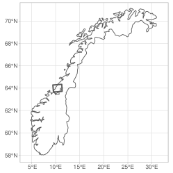
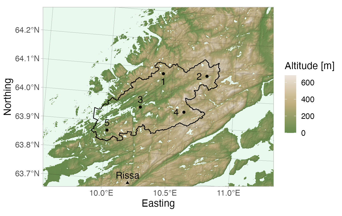
Figure 1: Left plot: Map of Norway with a square defining the spatial domain $\mathcal{S}$. Right plot: Elevation map of $\mathcal{S}$. The Rissa radar is displayed at the bottom of the map, and the five conditioning sites used in Section 4 are enumerated and marked by black circles. The Stordalselva catchment is displayed using a black polygon.

We use the radar precipitation maps for modelling and simulating extreme hourly precipitation over the Stordalselva catchment, located close to the Rissa radar. To achieve this, we download all data for 2010–2022 inside a spatial domain $\mathcal{S}$ of size $91\times 71=6461$ km², centred around the Stordalselva catchment. Figure 1 displays the domain $\mathcal{S}$ and the locations of the Rissa radar and the Stordalselva catchment. The spatial conditional extremes model allows one to model and simulate extremes occurring at any site of interest, by conditioning on that site experiencing extreme behaviour (see Section 3 for more details). For the sake of illustration, we choose five such conditioning sites, somewhat equally spaced throughout the water catchment, for modelling and simulating extreme precipitation in Section 4. These sites are also displayed in Figure 1. There are considerable differences between extreme summer precipitation and extreme winter precipitation in Norway [76], and we therefore choose to only model summer precipitation from June, July and August, which is when most of the intense precipitation events occur in Norway. There are some distortions in the data close to the Rissa radar, so we remove all observations from locations that are within $5$ km from the radar.

It can be difficult to distinguish between little and no precipitation using reflectivity data, and the estimated precipitation data contain both exact zeros and values with magnitudes as small as $10^{-5}$ mm/h. In the Supplementary Material [115], we show that there are large differences in the proportions of exact zeros for different times, due to an upgrade of the weather radar in 2018, but that the proportion of observations smaller than $0.1$ mm/h is approximately constant in time. We therefore round every observation smaller than $0.1$ mm/h down to zero.

3 Model framework

3.1 Model overview

We model the spatial extremal dependence structure of the hourly precipitation process, $X_{t}(\bm{s})$, at location $\bm{s}\in\mathcal{S}\subset\mathbb{R}^{2}$ and time $t\in\mathcal{T}\subset\mathbb{N}$, using the spatial conditional extremes model [120]. The model describes the conditional distribution of $X_{t}(\bm{s})$ given that $X_{t}(\bm{s}_{0})>\tau_{t}(\bm{s}_{0})$, where $\bm{s}_{0}$ is some chosen conditioning site and $\tau_{t}(\bm{s})$ is a large threshold that may vary in space and time. The conditioning site can be located anywhere in $\mathcal{S}$, which makes us free to place $\bm{s}_{0}$ at a specific location of interest, for modelling and simulating only the extremes that we care about.

To use the spatial conditional extremes model, we must first transform $X_{t}(\bm{s})$ into a standardised process $\tilde{X}_{t}(\bm{s})$, with Laplace marginal distributions at all locations and time points in $\mathcal{S}\times\mathcal{T}$, using the probability integral transform $\tilde{X}_{t}(\bm{s})=F^{-1}[F_{\bm{s},t}(X_{t}(\bm{s}))],$ where $F^{-1}$ is the quantile function of the Laplace distribution and $F_{\bm{s},t}$ is the cumulative distribution function of $X_{t}(\bm{s})$ [92]. However, the marginal distribution of hourly precipitation contains a point mass at zero, which means that the marginal distribution of $\tilde{X}_{t}(\bm{s})$ also contains a point mass, making it different from the Laplace distribution in its lower tail. [104, 105] tackle this problem by left-censoring all zeros. This yields promising results, but the censoring makes high-dimensional inference computationally intractable without the use of low-dimensional composite likelihoods. Moreover, this approach is still computationally demanding as it relies on evaluating bivariate Gaussian distributions many times. We therefore propose another approach for modelling $X_{t}(\bm{s})$ with the spatial conditional extremes model. Assume that hourly precipitation can be represented as $X_{t}(\bm{s})=X^{+}_{t}(\bm{s})I_{t}(\bm{s}),$ where $X^{+}_{t}(\bm{s})=[X_{t}(\bm{s})\mid X_{t}(\bm{s})>0]$ represents precipitation intensity and $I_{t}(\bm{s})$ is a binary random process that equals $1$ when $X_{t}(\bm{s})>0$ and $0$ when $X_{t}(\bm{s})=0$. So-called Richardson-type stochastic weather generators depend on this formulation by first simulating the precipitation occurrence $I_{t}(\bm{s})$ and then simulating the precipitation intensity $X^{+}_{t}(\bm{s})$ if $I_{t}(\bm{s})=1$ [106]. We build upon this approach by, instead of modelling $[X_{t}(\bm{s})\mid X_{t}(\bm{s})>\tau_{t}(\bm{s})]$, performing separate modelling of the conditional intensity process $[X^{+}_{t}(\bm{s})\mid X_{t}(\bm{s})>\tau_{t}(\bm{s})]$ and the conditional occurrence process $[I_{t}(\bm{s})\mid X_{t}(\bm{s})>\tau_{t}(\bm{s})]$, and then setting

$$\left[X_{t}(\bm{s})\mid X_{t}(\bm{s})>\tau_{t}(\bm{s})\right]=\left[X^{+}_{t}(\bm{s})I_{t}(\bm{s})\mid X_{t}(\bm{s})>\tau_{t}(\bm{s})\right].$$ (1)

The marginal distribution $F^{+}_{\bm{s},t}$, of $X^{+}_{t}(\bm{s})$, does not contain a point mass, so it can more easily be transformed into the Laplace distribution. Thus, we describe the conditional intensity process with the spatial conditional extremes model, while the conditional occurrence process is described with a suitable binary model. Our model for $F^{+}_{\bm{s},t}$ is described in Section 3.3. Then, our model for the conditional intensity process is described is Section 3.4, and our model for the conditional occurrence process is described in Section 3.5. Most of our models fall within the framework of latent Gaussian models, which are introduced in Section 3.2.

3.2 Latent Gaussian Models

A latent Gaussian model is a model where the observations $\bm{y}={(y_{1},y_{2},\ldots,y_{n})}^{\top}$ are assumed to be conditionally independent given a latent Gaussian random field $\bm{x}={(x_{1},x_{2},\ldots,x_{m})}^{\top}$ and a set of hyperparameters $\bm{\theta}_{1}$, namely

$$\left[\bm{y}\mid\bm{x},\bm{\theta}_{1}\right]\sim\prod_{i=1}^{n}\pi(y_{i}\mid\eta_{i}(\bm{x}),\bm{\theta}_{1}),\qquad\left[\bm{x}\mid\bm{\theta}_{2}\right]\sim\mathcal{N}(\mu(\bm{\theta}_{2}),\bm{Q}^{-1}(\bm{\theta}_{2})),$$

where the likelihood $\prod_{i=1}^{n}\pi(y_{i}\mid\eta_{i}(\bm{x}),\bm{\theta}_{1})$ is a parametric distribution with parameters $\eta_{i}(\bm{x})$ and $\bm{\theta}_{1}$, the linear predictor $\eta_{i}(\bm{x})$ is a linear combination of the elements in $\bm{x}$ and the latent field $\bm{x}$ is conditionally Gaussian with mean vector $\bm{\mu}$ and precision matrix $\bm{Q}$, given the hyperparameters $\bm{\theta}_{2}$. The prior distributions of $\bm{\theta}_{1}$ and $\bm{\theta}_{2}$ are $\pi(\bm{\theta}_{1})$ and $\pi(\bm{\theta}_{2})$, respectively.

The latent Gaussian modelling framework is highly flexible, as the likelihood can stem from an essentially arbitrary parametric distribution, while information from explanatory variables and a large variety of dependency structures can be incorporated into the linear predictor $\eta_{i}(\bm{x})$. Additionally, non-Gaussian structures can be incorporated into the model through the likelihood and the hyperparameters $\bm{\theta}_{1}$ and $\bm{\theta}_{2}$, which can be given any kind of prior distributions. Another advantage of the latent Gaussian model framework is that it allows for fast approximate inference using INLA, which is implemented in the R-INLA package [116, 117]. The package contains a large range of pre-implemented model components for the linear predictor, including splines, AR-models, random walk models and the so-called stochastic partial differential equation (SPDE) model of [96], which produces sparse approximations of Gaussian random fields with Matérn autocorrelation function

$$\gamma(d)=\frac{1}{2^{\nu-1}\Gamma(\nu)}{(\kappa d)}^{\nu}K_{\nu}(\kappa d),$$ (2)

where $d$ is the distance between two locations, $\nu>0$ is the smoothness parameter, $\rho=\sqrt{8\nu}/\kappa$ is the range parameter and $K_{\nu}$ is the modified Bessel function of the second kind and order $\nu$. Thus, R-INLA and the latent Gaussian model framework make it easy to quickly develop and perform inference with complex models for a large variety of applications.

3.3 Modelling the marginals

We model marginal distributions of the intensity process $X^{+}_{t}(\bm{s})$ by first modelling the bulk of the data with the gamma distribution, and then the upper tail with the GP distribution. Specifically, we model margins as

$$F^{+}_{\bm{s},t}(x)=\begin{cases}G_{\bm{s},t}(x)&x\leqslant u_{t}(\bm{s}),\\ G_{\bm{s},t}(u_{t}(\bm{s}))+(1-G_{\bm{s},t}(u_{t}(\bm{s})))H_{\bm{s},t}(x-u_{t}(\bm{s}))&x>u_{t}(\bm{s}),\end{cases}$$ (3)

where $G_{\bm{s},t}$ and $H_{\bm{s},t}$ are cumulative distribution functions of the gamma and GP distributions respectively, both with parameters that might vary in space and time, while $u_{t}(\bm{s})$ is the $p_{u}$-quantile of $G_{\bm{s},t}$, for some large probability $p_{u}$. This “split-modelling” approach is a common choice for modelling precipitation when aiming to describe both the bulk and the upper tail of the distribution [100, e.g.,]. We use the gamma and GP parametrisations of [69], which give a probability density function for the gamma distribution on the form

$$g(x)=\frac{x^{\kappa-1}}{\Gamma(\kappa)}{\left(\frac{G^{-1}(\alpha;\kappa,1)}{\psi_{\alpha}}\right)}^{\kappa}\exp{\left(\frac{G^{-1}(\alpha;\kappa,1)}{\psi_{\alpha}}\right)},\quad x>0,\quad\kappa,\psi_{\alpha}>0$$

where $\kappa$ is the standard shape parameter, $\alpha$ is a fixed probability, $G^{-1}(\alpha;\kappa,1)$ is the $\alpha$-quantile of a gamma distribution with shape $\kappa$ and scale $1$, and $\psi_{\alpha}$ is the $\alpha$-quantile of the gamma distribution. Using this parametrisation for the likelihood of our latent Gaussian model lets us directly estimate the $\alpha$-quantile of the data through the parameter $\psi_{\alpha}$. The GP distribution has cumulative distribution function

$$H(x)=\begin{cases}1-{\left(1+\left\{{(1-\beta)}^{-\xi}-1\right\}\frac{x}{\phi_{\beta}}\right)}_{+}^{-1/\xi},&\xi\neq 0,\\ 1-{(1-\beta)}^{x/\phi_{\beta}},&\xi=0,\end{cases}\quad\phi_{\beta}>0,\xi\in\mathbb{R},$$

with ${(a)}_{+}=\max(0,a)$, where $\xi$ is the tail parameter of the GP distribution, $\beta$ is a fixed probability and the parameter $\phi_{\beta}$ equals the $\beta$-quantile of the GP distribution. The support of the GP distribution is $(0,\infty)$ for $\xi\geqslant 0$, while it is $\left(0,\phi_{\beta}\left\{1-{(1-\beta)}^{-\xi}\right\}\right)$ for $\xi<0$.

We estimate the parameters of $G_{\bm{s},t}$ and $H_{\bm{s},t}$ separately, with two different latent Gaussian models. For the parameters of $G_{\bm{s},t}$, we use a latent Gaussian model with a gamma likelihood, where the shape parameter $\kappa$ is a hyperparameter that is constant in space and time, while $\psi_{\alpha}$ is allowed to vary in space and time through the linear predictor $\eta=\log\psi_{\alpha}$. Setting $\alpha=p_{u}$ lets us directly estimate the threshold $u_{t}(\bm{s})$, while estimating the parameters of $G_{\bm{s},t}$. The value of $p_{u}$, the components of $\eta$ and the priors for $\bm{\theta}$ vary depending on the application, and are therefore described in Section 4.1. After having performed inference with R-INLA, we estimate the parameters of $G_{\bm{s},t}$ as the posteriors means of $\kappa$ and $\psi_{\alpha}$.

Having estimated the threshold $u_{t}(\bm{s})$, we then model the distribution $H_{\bm{s},t}$ of the threshold exceedances $[X^{+}_{t}(\bm{s})-u_{t}(\bm{s})\mid X^{+}_{t}(\bm{s})>u_{t}(\bm{s})]$ with the GP distribution. Here, we apply a latent Gaussian model with a GP likelihood, where the tail parameter $\xi$ is a hyperparameter that is constant in space and time, while the linear predictor is $\eta=\log\phi_{\beta}$, where we set $\beta=0.5$, so that $\phi_{\beta}$ is the GP median. Once more, the parameters of $H_{\bm{s},t}$ are estimated as the posterior means of $\xi$ and $\phi_{\beta}$. Note that the GP likelihood within R-INLA only allows for modelling $\xi>0$. However, this should not be too problematic when modelling hourly precipitation data, as there is considerable evidence in the literature that precipitation is heavy-tailed, and thus it should be modelled with a non-negative tail parameter, especially for short temporal aggregation times [72, 112, 103, 85].

3.4 Spatial modelling of the conditional intensity process

We transform the precipitation intensities $X^{+}_{t}(\bm{s})$ into the standardised process $Y_{t}(\bm{s})$, with Laplace marginal distributions, using the probability integral transform, $Y_{t}(\bm{s})=F^{-1}[F^{+}_{\bm{s},t}(X^{+}_{t}(\bm{s}))]$. Given a conditioning site $\bm{s}_{0}$ and a threshold $\tau_{t}(\bm{s}_{0})$, we then model the spatial distribution of $Y_{t}(\bm{s})$ given that $X_{t}(\bm{s}_{0})>\tau_{t}(\bm{s}_{0})$, which is the same conditioning event as $Y_{t}(\bm{s}_{0})>F^{-1}[F^{+}_{\bm{s}_{0},t}(\tau_{t}(\bm{s}_{0}))]$. We assume that the notion of “extremes” can vary across time and space on the original precipitation scale, but not on the transformed Laplace scale. We therefore set $\tau_{t}(\bm{s}_{0})$ equal to a chosen quantile of $F^{+}_{\bm{s}_{0},t}$, which gives the constant threshold $\tau=F^{-1}[F^{+}_{\bm{s}_{0},t}(\tau_{t}(\bm{s}_{0}))]$ on the Laplace scale. The spatial conditional extremes model of [110] now states that, for $\tau$ large enough, the conditional process $\left[Y_{t}(\bm{s})\mid Y_{t}(\bm{s}_{0})=y_{0}>\tau\right]$ is Gaussian,

$$\left[Y_{t}(\bm{s})\mid Y_{t}(\bm{s}_{0})=y_{0}>\tau\right]\overset{d}{=}a(\bm{s};\bm{s}_{0},y_{0})+b(\bm{s};\bm{s}_{0},y_{0})Z_{t}(\bm{s};\bm{s}_{0})+\varepsilon_{t}(\bm{s};\bm{s}_{0}),$$ (4)

where $a(\cdot)$ and $b(\cdot)$ are two standardising functions, $Z_{t}(\bm{s};\bm{s}_{0})$ is a spatial Gaussian random field with $Z_{t}(\bm{s}_{0};\bm{s}_{0})=0$ almost surely, and $\varepsilon_{t}(\bm{s};\bm{s}_{0})$ is Gaussian white noise with $\varepsilon_{t}(\bm{s}_{0};\bm{s}_{0})=0$ almost surely. This is the same as a latent Gaussian model with a Gaussian likelihood and latent field $a(\cdot)+b(\cdot)Z(\cdot)$, which means that computationally efficient approximate inference can be performed using INLA. [110] demonstrate how to perform efficient high-dimensional inference by using R-INLA and modelling $Z_{t}(\bm{s};\bm{s}_{0})$ with the SPDE approximation. [114] build upon their work and develop a methodology for implementing computationally efficient parametric models for $a(\bm{s};\bm{s}_{0})$ and $b(\bm{s};\bm{s}_{0})$ in R-INLA and a method for efficient constraining of $Z_{t}(\bm{s};\bm{s}_{0})$ such that $Z_{t}(\bm{s}_{0};\bm{s}_{0})=0$ almost surely. We apply their methodology for modelling the spatial distribution of conditional precipitation extremes, while developing new diagnostics and models for the standardising functions $a(\cdot)$ and $b(\cdot)$.

3.5 Spatial modelling of the conditional occurrence process

Four competing models are applied to describe the spatial distribution of conditional precipitation occurrences, $\left[I_{t}(\bm{s})\mid X_{t}(\bm{s}_{0})>\tau_{t}(\bm{s}_{0})\right]$. One of these is the relatively common spatial probit model, which assumes that $I_{t}(\bm{s})$ depends on an underlying latent Gaussian process $Z_{t}(\bm{s})$ such that $I_{t}(\bm{s})=1$ when $Z_{t}(\bm{s})+\varepsilon_{t}(\bm{s})\geqslant 0$ and $I_{t}(\bm{s})=0$ otherwise, where $\varepsilon_{t}(\bm{s})$ is zero-mean Gaussian white noise. Thus, the process $I_{t}(\bm{s})$ is conditionally independent given $Z_{t}(\bm{s})$, with success probability $\text{P}\left[I_{t}(\bm{s})=1\mid Z_{t}(\bm{s})\right]=\Phi(Z_{t}(\bm{s})/\sigma)$, where $\Phi(\cdot)$ is the cumulative distribution function of the standard normal distribution and $\sigma^{2}$ is the variance of $\varepsilon_{t}(\bm{s})$. This means that the probit model is in fact a latent Gaussian model with a Bernoulli likelihood, and that we can perform fast inference using INLA. Within R-INLA, we decompose $Z_{t}(\bm{s})$ into $Z_{t}(\bm{s})=\mu(\bm{s})+Z^{*}_{t}(\bm{s})$, where $Z^{*}_{t}(\bm{s})$ is a zero-mean Gaussian random field, and $\mu(\bm{s})$ describes the mean of $Z_{t}(\bm{s})$. For faster inference, we model $Z_{t}^{*}(\bm{s})$ with the SPDE approximation. Assuming stationarity, we enforce $I_{t}(\bm{s}_{0})=1$ by modelling $\mu(\bm{s})$ as a function of the distance $d$ between $\bm{s}$ and $\bm{s}_{0}$, i.e., $\mu(d)\equiv\mu(\bm{s})$ with $d=\|\bm{s}-\bm{s}_{0}\|$. Then we ensure that $\mu(0)$ is positive and large, while also enforcing that $Z^{*}_{t}(\bm{s}_{0})=0$ almost surely, using the constraining method of [114]. This does not guarantee that P$(I_{t}(\bm{s}_{0})=1)=1$ exactly, but if $\mu(0)$ is large enough, then P$(I_{t}(\bm{s}_{0})=1)\approx 1$ for most practical purposes. The exact structure of $\mu(\bm{s})$ varies depending on the application in question.

The spatial probit model can produce realistic realisations of the spatial binary process, but it can also struggle in situations where the binary field is smooth, in the sense that the variance of $\varepsilon_{t}(\bm{s})$ is considerably smaller than the variance of $Z_{t}(\bm{s})$. To ensure smooth model realisations, the variance of $Z_{t}(\bm{s})/\sigma$ must become so large that the probability $\Phi(Z_{t}(\bm{s})/\sigma)$ always is close to either 0 or 1, and this large variance can make it difficult to reliably estimate trends in the mean $\mu(\bm{s})$. For this reason, we also attempt to model the conditional occurrence process using a probit model without any spatial effects, i.e., where we remove $Z_{t}^{*}(\bm{s})$. This model typically fails at providing realistic-looking realisations of smooth binary processes, but it can perform considerably better at capturing trends in the mean structure.

Our probit models are independent of the conditional intensity model, so it is possible for the simulated occurrence samples to create highly non-smooth precipitation realisations where areas with large precipitation values suddenly contain a “hole” of zeros close to the most extreme observations. This is an unrealistic behaviour that we wish to avoid. Our third modelling strategy is therefore based on the assumption that the occurrence process is dependent upon the intensity process such that only the smallest values of $X_{t}^{+}(\bm{s})$ gets turned into zeros. Thus, the third approach, denoted the threshold model, estimates the overall probability $p$ of observing zeros in the data, and then set $I_{t}(\bm{s})$ equal to zero whenever $X_{t}^{*}(\bm{s})$ is smaller than its estimated $p$-quantile. Lastly, for improved base-line comparisons, we add a fourth occurrence model, which interprets “no precipitation” as a tiny but positive amount of precipitation, i.e., $I_{t}(\bm{s})\equiv 1$. We denote this the nonzero model.

4 Simulating extreme hourly precipitation

We apply the models from Section 3 to the data from Section 2 for modelling and simulating spatial realisations of extreme hourly precipitation. In Section 4.1 we model and standardise the marginal distributions of the data. Then, in Section 4.2 and Section 4.3, we model the conditional intensities and occurrences of extreme precipitation, respectively. Finally, in Section 4.4, we combine all the model fits for simulating spatial realisations of extreme hourly precipitation.

4.1 Modelling the marginals

We model the marginal distribution $F^{+}_{\bm{s},t}$ of nonzero precipitation using the gamma-GP split-model from Section 3.3, where we choose $\alpha=p_{u}=0.95$. We attempt to model the linear predictor using a separable space-time model where the spatial effect is modelled with a spatial Gaussian random field, described using the SPDE approximation, and the temporal effect is modelled with a Gaussian smoothing spline, also described using the SPDE approximation. However, we find that the spatial effect is estimated to be almost constant, and that a purely temporal model using only the Gaussian smoothing spline performs better. We therefore decide to use the purely temporal model, where the linear predictor is equal to a temporal Gaussian smoothing spline. A model based on splines is unsuitable for prediction outside the observed spatio-temporal domain, but the aim of this paper is modelling, and not forecasting, so we find it to be a good model choice.

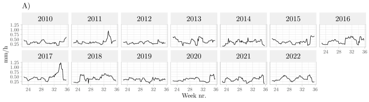
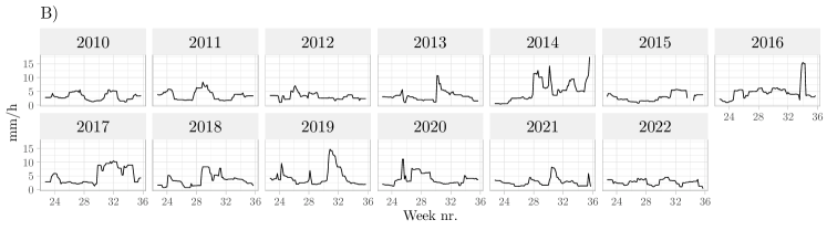
Figure 2: Estimators for the $95\%$-quantile of hourly precipitation intensity (A) and the median of precipitation threshold exceedances (B) for each summer day during 2010–2022. In black: empirical estimators created using a sliding window of width of one week. In red: posterior means estimated using the latent Gaussian models with a gamma likelihood (A) and a GP likelihood (B).

We place the weakly informative penalised complexity (PC) prior [109] of [80] on the range $\rho=\sqrt{8\nu}/\kappa$ and variance $\sigma^{2}$ such that the prior probability that $\rho$ exceeds $28$ days is $5\%$ and the prior probability that $\sigma$ exceeds a value of $3$ is $5\%$. The smoothness parameter $\nu$ can be difficult to estimate [95], so we fix it to $\nu=1.5$. Due to the large amounts of data, we speed up inference by only using observations from a spatial subgrid of the data with resolution $2\times 2$ km².

Inference is performed with R-INLA, in approximately half an hour, when using only one core on a 2.6 gHz Linux server. The posterior mean of the shape parameter $\kappa$ equals $0.69$, and the posterior mean of the threshold $u_{t}(\bm{s})$ is displayed in Subplot A of Figure 2, together with the empirical $95\%$-quantiles of the precipitation intensities, pooled across space. The smoothing spline seems to capture the temporal trends of the data well. We evaluate the model fit using quantile-quantile (QQ) plots. These are displayed in the Supplementary Material [115], and they show an almost perfect correspondence between model quantiles and empirical quantiles. We conclude that the model fit is satisfactory.

Having estimated $u_{t}(\bm{s})$, we then model the threshold exceedances $[X^{+}_{t}(\bm{s})-u_{t}(\bm{s})\mid X^{+}_{t}(\bm{s})>u_{t}(\bm{s})]$ with the GP distribution, as described in Section 3.3. Once more, we find that a purely temporal model for the linear predictor performs better than a separable space-time model. We therefore model the linear predictor using a similar spline model as in the gamma model, with the same prior distributions. The tail parameter $\xi$ is given the PC prior of [100],

$$\pi(\xi)=\lambda(1-\xi/2){(1-\xi)}^{-3/2}2^{-1/2}\exp\left(-\lambda\xi/\sqrt{2(1-\xi)}\right),\quad 0\leqslant\xi<1,$$

with penalty parameter $\lambda$. The GP distribution has infinite mean for $\xi\geqslant 1$ and infinite variance for $\xi\geqslant 1/2$, and since it is well established in the literature that $\xi$ tends to be in the range between $0.05$ and $0.3$ for precipitation data [72, 112, 103, e.g.,], we enforce $\xi\leqslant 1/2$ to ease parameter estimation. Then, we choose $\lambda=7$, which gives the prior probability P$(\xi\leqslant 0.4)\approx 95\%$.

Inference is performed with R-INLA, using all the spatial locations, in approximately 2 minutes. The posterior mean of $\xi$ is $0.145$, which is far away from the upper bound of $1/2$, and corresponds well with the results of [113], who estimated $\xi=0.18$ with a $95\%$ credible interval of $(0.14,0.21)$ when modelling the yearly maxima of hourly precipitation using rain gauge data from a spatial domain that covers $\mathcal{S}$. Subplot B of Figure 2 displays the empirical median of the threshold exceedances, pooled in space, along with the posterior means of the threshold exceedance medians, which seem to agree well with the main temporal trends of the data. We evaluate the model fit using QQ plots, displayed in the Supplementary Material [115]. These demonstrate a good correspondence between model quantiles and empirical quantiles. We once more conclude that our model provides a satisfactory fit to the data.

4.2 Modelling the conditional intensity process

We standardise the precipitation intensities to have Laplace marginal distributions. Then, following [92], we choose the functions $a(\bm{s};\bm{s}_{0},y_{0})=\alpha(\bm{s};\bm{s}_{0})y_{0}$ and $b(\bm{s};\bm{s}_{0},y_{0})=y_{0}^{\beta(\bm{s};\bm{s}_{0})}$ for the spatial conditional extremes model (4), which, they claim, can cover a large range of dependence structures, including all the standard copulas studied by [90] and [99]. Building upon the work of [114], we develop new empirical diagnostics for making informed decisions about the value of the threshold $\tau$ and the forms of $\alpha(\bm{s};\bm{s}_{0})$ and $\beta(\bm{s};\bm{s}_{0})$.

We assume that the standardising functions only depend on the Euclidean distance to $s_{0}$ and define $\alpha(d)\equiv\alpha(\bm{s};\bm{s}_{0})$ with $d=\|\bm{s}-\bm{s}_{0}\|$, and similarly for $\beta(d)$. Assuming that the residual field $Z_{t}(\bm{s};\bm{s}_{0})$ is isotropic, we denote the mean and variance of $[Y_{t}(\bm{s})\mid Y_{t}(\bm{s}_{0})=y_{0}]$ as $\mu(d;y_{0})$ and ${\zeta(d;y_{0})}^{2}$, respectively. Under the spatial conditional extremes model (4), these equal $\mu(d;y_{0})=\alpha(d)y_{0}$ and ${\zeta(d;y_{0})}^{2}={\sigma(d)}^{2}y_{0}^{2\beta(d)}+\sigma_{\varepsilon}^{2}$, where $\sigma_{\varepsilon}^{2}$ is the variance of the nugget term $\varepsilon_{t}(\bm{s};\bm{s}_{0})$ and ${\sigma(d)}^{2}$ is the variance of $Z_{t}(\bm{s};\bm{s}_{0})$ when $\|\bm{s}-\bm{s}_{0}\|=d$. By computing the empirical mean, $\hat{\mu}(d;y_{0})$, of the conditional precipitation intensity, we can estimate $\alpha(d)$ as $\hat{\alpha}(d;y_{0})=\hat{\mu}(d;y_{0})/y_{0}$. Similarly, by assuming that $\sigma_{\varepsilon}$ is small, we can estimate $\beta(d)$ using empirical conditional variances as

$$\hat{\beta}(d;y_{0},y_{1})=\log\{\hat{\zeta}(d;y_{0})/\hat{\zeta}(d;y_{1})\}/\log(y_{0}/y_{1}),$$

where $\hat{\zeta}(d;y)$ is the empirical standard deviance of all observations with distance $d$ to a conditioning site with threshold exceedance $y$, and $y_{0}\neq y_{1}$ are any two threshold exceedances $y_{0},y_{1}>\tau$. This allows us to create multiple different estimators $\hat{\alpha}(d;y_{0})$ and $\hat{\beta}(d;y_{0},y_{1})$ for $\alpha(d)$ and $\beta(d)$, respectively, by varying the values of $y_{0}$ and $y_{1}$. This provides a diagnostic for estimating the threshold $\tau$, since the spatial conditional extremes model assumes that $\alpha(d)$ and $\beta(d)$ are constant for all threshold exceedances larger than $\tau$. Thus, we compute $\hat{\alpha}(d;y_{0})$ and $\hat{\beta}(d;y_{0},y_{1})$ for a large range of values of $y_{0}$ and $y_{1}$, and we set $\tau$ equal to the smallest value such that the estimators are approximately constant for all $y_{0},y_{1}>\tau$. Then, we propose parametric functions for $\alpha(d)$ and $\beta(d)$ that can fit well to the patterns that we find in the empirical estimators. Finally, we also compute $\hat{\sigma}(d;y_{0},y_{1})=\hat{\zeta}(d;y_{0})y_{0}^{-\hat{\beta}(d;y_{0},y_{1})}$ to get an idea about the marginal variances of the residual process $Z(\bm{s};\bm{s}_{0})$.

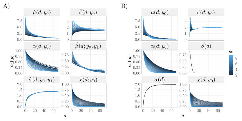
Figure 3: A) Empirical moments and estimators for $\chi(d;y_{0})$ and components of the conditional extremes model (4). B) Posterior means of the same variables from the model fit based on conditioning site nr. 2.

Exploratory analysis hints at some weak anisotropy in the precipitation data. However, we do not believe the lack of isotropy is strong enough to cause considerable problems, and the development of a suitable anisotropic model is outside the scope of this paper. We therefore assume an isotropic model. We compute $\hat{\mu}(d;y_{0})$ and $\hat{\zeta}(d;y_{0})$ with a sliding window approach. For any value of $d$ and $y_{0}$, the moments are estimated using all observations within a distance $d\pm 0.5$ km from a location where a value of $\log(y_{0})\pm 0.025$ is observed. We then compute $\hat{\alpha}(d;y_{0})$, $\hat{\beta}(d;y_{0},y_{1})$ and $\hat{\sigma}(d;y_{0},y_{1})$ as previously described, where we fix $y_{1}$ to the $90\%$-quantile of the Laplace distribution. We also estimate empirical conditional exceedance probabilities $\chi(d;y_{0})\equiv\chi_{p}(\bm{s},\bm{s}_{0})$, where $d=\|\bm{s}-\bm{s}_{0}\|$ and $p=F^{-1}(y_{0})$ with $F^{-1}$ the quantile function of the Laplace distribution, using a similar sliding window approach. All the estimators are displayed in subplot A of Figure 3. The estimated shape of $\sigma(d)$ corresponds well with the standard deviation of a random field with constant variance, constrained to be zero at $\bm{s}_{0}$. The estimators for $\alpha(d)$ seem to behave like functions with exponential-like decay towards zero as $d$ increases. However, the decay occurs at an increasing rate as $y_{0}$ increases, and it never seems to stabilise as a function of $y_{0}$. This indicates that, with the available amounts of data, we cannot choose a large enough threshold $\tau$ such that the function $a(d;y_{0})=\alpha(d)y_{0}$ provides a good fit for all $y_{0}>\tau$. Therefore, we instead propose to model the mean as $a(d;y_{0})=\alpha(d;y_{0})y_{0}$, where the function $\alpha(\cdot)$ depends on both distance $d$ and intensity level $y_{0}$, and we choose a relatively low threshold, $\tau=y_{1}$.

A common model for $\alpha(d)$ is $\alpha(d)=\exp\{-{(d/\lambda_{a})}^{\kappa_{a}}\}$, with $\lambda_{a},\kappa_{a}>0$, see, e.g, [120], [104] and [111]. We therefore examine if the model $\alpha(d;y_{0})=\exp[-{\{d/\lambda_{a}(y_{0})\}}^{\kappa_{a}(y_{0})}]$ can provide a good fit to our data, where $\lambda_{a}(y_{0})$ and $\kappa_{a}(y_{0})$ are parametric functions of $y_{0}$. Using a sliding window approach, we estimate $\lambda_{a}(y_{0})$ and $\kappa_{a}(y_{0})$ by minimising the sum of squared errors between $[Y(\bm{s})\mid Y(\bm{s}_{0})=y_{0}]$ and $a(\|\bm{s}-\bm{s}_{0}\|;y_{0})$ for different values of $y_{0}$. These least squares estimators are displayed in the Supplementary Material [115]. Based on our findings we propose to model $\lambda_{a}(y_{0})$ as $\lambda_{a}(y_{0})=\lambda_{a0}\exp(-(y_{0}-\tau)/\Lambda_{\lambda})$, with $\lambda_{a0},\Lambda_{\lambda}>0$, and $\kappa_{a}(y_{0})$ as $\kappa_{a}(y_{0})=\kappa_{a0}\exp(-{((y_{0}-\tau)/\Lambda_{\kappa})}^{\varkappa})$, with $\kappa_{a0},\Lambda_{\kappa},\varkappa>0$.

The estimators for $\beta(d)$ in subplot A of Figure 3 have a clear dependence on $y_{0}$ at short distances $d$. However, $\hat{\beta}(d;y_{0},y_{1})$ seems to be independent of $y_{0}$ for longer distances, and the changes as a function of $y_{0}$ are much less severe than those in $\hat{\alpha}(d;y_{0})$. We therefore stick to a model on the form $b(d;y_{0})=y_{0}^{\beta(d)}$. Based on the estimators in subplot A of Figure 3, it seems that $\beta(d)$ should be modelled with a function that decays exponentially towards zero. We therefore choose the model $\beta(d)=\beta_{0}\exp(-{(d/\lambda_{b})}^{\kappa_{b}})$ with $\lambda_{b},\kappa_{b}>0$ and $\beta_{0}\in[0,1)$.

Having chosen the threshold $\tau$ and parametric forms for the functions $a(d;y_{0})$ and $b(d;y_{0})$, we then apply the method of [114] for defining a nonstationary and constrained SPDE approximation to the spatial Gaussian random field in (4) within R-INLA. This SPDE model approximates spatial Gaussian random fields on the form $b(\bm{s};\cdot)Z(\bm{s})$ as a linear combination of $m$ Gaussian mesh nodes, $\hat{Z}_{b}(\bm{s})=\sum_{i=1}^{m}\phi_{i}(\bm{s})b_{i}W_{i}$, where $b_{1},b_{2},\ldots,b_{m}$ are the values of the function $b(\bm{s})$ at the location of the $m$ mesh nodes, and $\phi_{i}$ and $W_{i}$ are basis functions and Gaussian mesh nodes from the “standard” SPDE approximation, $\hat{Z}(\bm{s})=\sum_{i=1}^{m}\phi_{i}(\bm{s})W_{i}$, of [96]. The nonstationary SPDE approximation is then constrained at $\bm{s}_{0}$ by placing one of the mesh nodes at $\bm{s}_{0}$, and constraining it to be exactly zero.

For each of the five chosen conditioning sites, we perform inference with R-INLA, using data from all time points where $\tau$ is exceeded at $\bm{s}_{0}$ and all 6404 locations in $\mathcal{S}$. In an empirical Bayes like approach, we place Gaussian priors on the logarithms of the parameters in $a(\cdot)$, with variance $5^{2}$ and means equal to their least squares estimators. For the parameters of $b(\cdot)$, we choose Gaussian priors with variance $5^{2}$ for $\log(\lambda_{b})$, $\log(\kappa_{b})$ and $\log(\beta_{0}/(1-\beta_{0}))$, which ensures $\lambda_{b},\kappa_{b}>0$ and $\beta_{0}\in(0,1)$. The prior means are chosen based on the diagnostics in Figure 3. We set them equal to $\log(8.5)$, $\log(0.5)$ and $\log(0.65/(1-0.65))$, respectively. The parameters of $Z_{t}(\bm{s})$ are given the PC prior of [80], such that the prior probability that the range $\rho$ exceeds $60$ km is $5\%$ and the prior probability that the standard deviation $\sigma$ exceeds $4$ is $5\%$. We fix the smoothness parameter to $\nu=0.5$, to represent our belief about the smoothness properties of extreme precipitation fields.

Inference with R-INLA is performed within 1–4 hours for each conditioning site, using only one core on the same Linux server as before. We evaluate the five model fits by estimating posterior means of the same variables as in subplot A of Figure 3, using $1000$ posterior samples of $\bm{\theta}$. Subplot B displays these posterior means from the model fit based on conditioning site nr. 2. Although there are some differences between subplot A and B, the patterns of the estimated curves are in general agreement, indicating a satisfactory model fit overall. The posterior mean of $\mu(d;y_{0})$ is similar to that of the data, with some slight underestimation for large values of $d$ and $y_{0}$. The standard deviation $\zeta(d;y_{0})$ is slightly underestimated for small $d$, and overestimated for large $d$. For the values of $\chi(d;y_{0})$, which we care the most about, this results in a weak underestimation for small $d$ and large $y_{0}$, and overestimation for large $d$ and small $y_{0}$. We believe that more complex models for $a(\cdot)$ and $b(\cdot)$, e.g., with $\beta(\cdot)$ being a function of $y_{0}$ at small $d$, would be able to further reduce the differences seen in Figure 3. However, for the scope of this paper, we deem that the current fit is good enough. We also believe that the combination of minor overestimation and underestimation of $\chi(\cdot)$ might somewhat cancel each other out. Estimators based on all five model fits are displayed in the Supplementary Material [115], and they all seem to capture the major trends of the data.

4.3 Modelling the conditional occurrence process

To model conditional precipitation occurrences, we first search for patterns in the observed data. Since we model $[I_{t}(\bm{s})\mid Y(\bm{s}_{0})>\tau]$, we expect the occurrence probability to be higher as we move closer to $\bm{s}_{0}$. We therefore compute empirical occurrence probabilities $\hat{p}(d)$ at different distances $d$ from $\bm{s}_{0}$, using a sliding window of width $1$ km. These are displayed by the black line in subplot B of Figure 4. As expected, $\hat{p}(d)$ decreases as $d$ increases, with an almost linear decline. Subplot A of Figure 4 displays six realisations of the precipitation data. The distribution of precipitation occurrence appears to be smooth in space, in the sense that zeros cluster together. Thus, the non-spatial probit model is unable to produce realistic looking simulations. The precipitation intensities also appear to be smooth in space, in the sense that we never observe big jumps in the precipitation values, and that zeros only occur next to other zeros or small precipitation values. To check if this is true for all the available data, we estimate the probability $p(\bar{y})$ of observing precipitation as a function of the mean observed precipitation $\bar{y}$ at the four closest spatial locations. The empirical estimator is displayed using the black line in subplot C of Figure 4. It seems that the probability of observing precipitation is close to zero if $\bar{y}=0$, and that it increases as a function of $\bar{y}$, and is almost exactly 1 if $\bar{y}>0.2$ mm/h. This implies that our probit models might produce unrealistic simulations, as they are independent of the intensity model and might produce zeros close to large precipitation values.

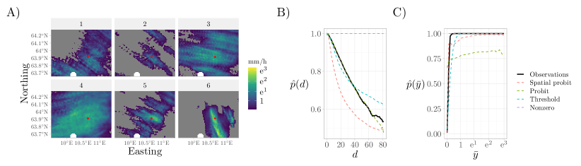
Figure 4: A) Visualisation of observed precipitation for six time points where a threshold exceedance is observed at conditioning site nr. 4 (marked by a red dot). Grey denotes zero precipitation, while white denotes observations close to the Rissa radar that have been removed. The rightmost plots display empirical estimates for $p(d)$ (B) and $p(\bar{y})$ (C), created using both observed data and simulated data from the four different occurrence models.

Based on the exploratory analysis, we model the mean $\mu(d)$, of the two probit models, using a spline. More specifically, we model $\partial\mu(d)/\partial d$ as a spline function based on 0-degree B-splines, where we place Gaussian zero-mean priors with a standard deviation of $10$ on all spline coefficients. Additionally, in the spatial probit model, we place PC priors on the SPDE parameters [80] such that the prior probability that the range parameter $\rho$ exceeds $70$ km is $5\%$ and the prior probability that the standard deviation of $Z^{*}_{t}(\bm{s})$ exceeds $5$ is $1\%$. The smoothness parameter is fixed to $\nu=0.5$. We then perform inference separately for each of the five chosen conditioning sites and the two probit models. Inference with R-INLA takes between 10–15 minutes for the spatial probit models, and 2–3 minutes for the non-spatial probit models. For the threshold model, we estimate the threshold by computing the empirical probabilities of observing precipitation inside the Stordalselva catchment given extremes at each of the five conditioning sites.

We evaluate model performance by comparing properties of observed and simulated data. The threshold model depends on the intensity process, so we first simulate conditional intensities, by sampling $\bm{\theta}$ from its posterior distribution and then sampling both $[Y_{t}(\bm{s}_{0})\mid Y_{t}(\bm{s}_{0})>\tau]$ and $\{Y_{t}(\bm{s})\mid Y_{t}(\bm{s}_{0}),\bm{\theta}:\bm{s}\in\mathcal{S}\}$ using (4). Then, we “simulate” occurrences with the threshold model by rounding all small enough precipitation intensities down to zero. Figure 4 displays empirical estimates for the probability of observing precipitation as a function of the distance $d$ to $\bm{s}_{0}$ and as a function of the mean $\bar{y}$ of the four nearest neighbours, for observed and simulated precipitation data. Clearly, the nonzero model fails to capture the probability of precipitation occurrences. From subplot B we find that the spatial probit model heavily underestimates the probability of observing precipitation for most distances $d$. The threshold model performs better than the spatial probit model, but it slightly underestimates $p(d)$ for small $d$ and overestimates it for large $d$. The non-spatial probit simulations, however, seem to agree well with the observed data for all values of $d$. From subplot C of Figure 4, we see that both probit models simulate zeros right next to large precipitation observations, resulting in an underestimation of $p(\bar{y})$. The spatial probit model performs better than the classical independent one, but it still does not completely solve this misfit. The threshold occurrence simulations, however, seem to agree well with the observations by placing its zeros close to other zeros or small precipitation values. Overall, the threshold model seems to be the best at estimating occurrence probabilities. The classical probit model is considerably better at estimating $p(d)$, but it completely fails at estimating $p(\bar{y})$.

4.4 Simulating spatial precipitation extremes

We combine all of the fitted models to simulate extreme precipitation over the Stordalselva catchment. For each of the five conditioning sites, extreme precipitation is simulated using Algorithm 1, with $N={10}^{3}$ samples, where Exp$(1)$ denotes the exponential distribution with unit scale, $\mathcal{S}_{1}\subset\mathbb{R}^{2}$ denotes all locations where we simulate extreme precipitation, $\hat{F}^{-1}_{t}$ denotes the estimated marginal quantile function of positive hourly precipitation at time $t$, and $F$ denotes the cumulative distribution function of the Laplace distribution. Recall that $\mathcal{T}$ is the set of all time points in our data.

Algorithm 1 Simulating spatial extreme precipitation with conditioning site $\bm{s}_{0}$.

Sample $N$ time points $t_{1},\ldots,t_{N}$ uniformly with replacement from $\mathcal{T}$.

for $i=1,2,\ldots,N$ do

     Sample a threshold exceedance $[Y_{i}(\bm{s}_{0})\mid Y_{i}(\bm{s}_{0})>\tau]\sim\tau+\text{Exp}(1)$

     Sample a spatial realisation of the conditional intensity process $\{Y_{i}(\bm{s}):\bm{s}\in\mathcal{S}_{1}\}\mid Y_{i}(\bm{s}_{0})$

     Sample a spatial realisation of the conditional occurrence process $\{I_{i}(\bm{s}):\bm{s}\in\mathcal{S}_{1}\}\mid Y_{i}(\bm{s}_{0})$

     Transform back to the precipitation scale: $X^{+}_{i}(\bm{s})=\hat{F}^{-1}_{t_{i}}[F(Y_{i}(\bm{s}))]$

     Add zeros to the samples: $X_{i}(\bm{s})=X^{+}_{i}(\bm{s})I_{i}(\bm{s})$

end for

Figure 5 displays observed and simulated realisations of extreme precipitation over the Stordalselva catchment. Simulations from the classical probit model and the nonzero model are not capturing the spatial structure of precipitation occurrence in the observed data, while simulations from the spatial probit model and the threshold model look more realistic. However, unlike the threshold model simulations, many of the spatial probit simulations contain large precipitation intensities right next to zeros, which is unrealistic.

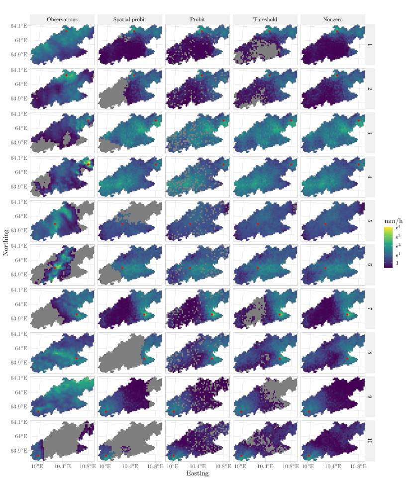
Figure 5: Realisations of conditional extreme precipitation, from observed and simulated data. The red dots display the locations of the chosen conditioning site for each subplot.

As discussed in Section 1, both the amount of precipitation and its spatial distribution are important features for assessing flood risk. Thus, to further evaluate the simulations, we compare conditional exceedance probabilities and precipitation sums over different areas between the observed and simulated data. Estimators for $\hat{\chi}_{p}(d)$ are computed using the same sliding window approach as in Section 4.2. Figure 6 displays the estimators from conditioning site nr. 1. The simulations seem to capture $\chi_{p}(d)$ well, even though, just as in Section 4.2, $\chi_{p}(d)$ is somewhat underestimated for small $d$ and overestimated for large $d$. The probit models seem to overestimate $\chi_{p}(d)$ less than the non-probit models at large distances, which makes sense, because the models are independent of the intensity process and thus can set large intensity values equal to zero. The estimators for $\chi_{p}(d)$ seem almost identical for the threshold model simulations and the nonzero model simulations. This also makes sense, since the small values that are rounded down to zero by the threshold model are too small to considerably affect the values of $\chi_{p}(d)$. Similar patterns are found for the other four conditioning sites. Estimators for $\chi_{p}(d)$ from all five conditioning sites are displayed in the Supplementary Material [115]. They all display similar patterns.

Figure 6: Estimators of $\chi_{p}(d)$ for observed and simulated data, using conditioning site nr. 1.

We also compare aggregated simulated and observed precipitation amounts over the Stordalselva catchment to evaluate the simulations. For each conditioning site, we compute precipitation sums inside $\mathcal{B}_{d}(\bm{s}_{0})\cap\mathcal{S}_{1}$, where $\mathcal{B}_{d}(\bm{s}_{0})$ is a ball of radius $d$ km, centred at $\bm{s}_{0}$, and $\mathcal{S}_{1}$ denotes the catchment of interest. We then compare observed and simulated precipitation sums using QQ plots. Figure 7 display these plots for conditioning site nr. 4. For small $d$, all the simulations produce similar precipitation amounts, which are close to the observed data, although slightly smaller. As $d$ increases, the underestimation increases somewhat for the probit models, while it decreases for the non-probit models, which seem to agree well with the observed data. Quantiles of the threshold model and the nonzero model are almost identical and can be hard to distinguish. QQ plots for all five conditioning sites are displayed in the Supplementary Material [115]. They all display similar patterns.

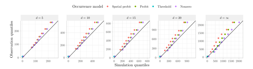
Figure 7: QQ plots for the sum of aggregated precipitation inside $\mathcal{B}_{d}(\bm{s}_{0})\cap\mathcal{S}_{1}$, based on conditioning site nr. 4. Quantiles from the four different simulated data sets are displayed using different colours.

5 Discussion and conclusion

We propose a framework for modelling and simulating high-dimensional spatial precipitation extremes, using the spatial conditional extremes model and latent Gaussian models. We model the marginal distributions of nonzero precipitation using a mixture of two latent Gaussian models with a gamma likelihood and a generalised Pareto (GP) likelihood, while separately modelling the extremal dependence of nonzero precipitation extremes with a spatial conditional extremes model formulated as a latent Gaussian model. Precipitation occurrences are modelled using four different competing binary models. Fast approximate inference is achieved using integrated nested Laplace approximations (INLA). We develop new empirical diagnostics for the threshold and standardising functions of the spatial conditional extremes model, and we use these to propose a new class of parametric forms for the standardising functions. The developed framework is applied for simulating high-resolution precipitation extremes over a water catchment in Central Norway, and is found to perform well.

The threshold occurrence model appears to outperform the other occurrence models, as it captures both spatial and marginal properties of the data well, whereas the two probit models fail to capture either the marginal or the spatial properties. However, since the precipitation simulations stem from a combination of intensity samples and occurrence samples, it is nontrivial to conclude that one occurrence model significantly outperforms the others, as a change in the intensity model might potentially cause another occurrence model to produce the best precipitation simulations.

Compared to the probit models, the threshold model lacks some flexibility in the sense that it produces deterministic simulations given the intensity samples and a threshold. However, the threshold model interacts with the intensity model, which the probit models are unable to. This interaction is clearly crucial, as the threshold model ends up being our most successful. For future work, it might prove fruitful to develop probit models that interact more with the intensity model. A common approach for creating such interactions is to perform joint inference, where the two models share some latent model components, similar to [64] and [81]. This might be challenging for the intensity and occurrence models, as their latent fields have different interpretations and scales, but it might still be possible to create some meaningful link between the two.

The spatial probit model underestimates occurrence probabilities almost everywhere in space. We believe this happens because the spatial clustering of zeros and ones in the data forces the nugget effect to be small, which, in the latent Gaussian model formulation, causes the latent field to have a large enough variance to absorb most of the mean trend. The symmetry of the latent field thus makes all marginal probabilities tend towards $50\%$, meaning that it underestimates large probabilities and overestimates small probabilities. One might fix this by removing the conditional independence assumption, i.e., discarding the nugget effect. However, this makes inference with INLA impossible. Alternatively, one might use an asymmetric latent random field, with a skewness that varies in space, so that latent variables close to the conditioning site are right skewed, while latent variables further away from the conditioning site are more left skewed. [68] show that inference with INLA can be possible for non-Gaussian latent fields, meaning that R-INLA might work with such a model. Future work should attempt to add changes in skewness to the latent field of the spatial probit model.

As discussed in Section 1, radar data are great for capturing the small-scale spatio-temporal variability of precipitation, but not many have used them for modelling extreme precipitation. We show that the radar data let us capture small-scale extremal dependence structures with high precision. However, it weather radars are known to struggle with capturing the exact precipitation amounts, i.e., marginal distributions, well. This might negatively affect our estimates of aggregated precipitation amounts. Thus, to create reliable simulations of extreme precipitation, future work should attempt to combine information from multiple precipitation data sets, by, e.g., modelling extremal dependence using high-density radar data, while modelling marginal distributions using rain gauge observations, which are better at capturing the marginal distributions of precipitation, but that are too sparse in space to provide successful estimates of the extremal dependence structure.

Our models assume isotropy, but the observed data in Figures 4 and 5 display some indications of anisotropy. This does not seem to affect our results much, as the simulated data capture the main trends of the observed data well. However, future work should attempt to add features of anisotropy and/or nonstationarity into the model framework, which is possible within the SPDE and R-INLA frameworks [94].

It is known that R-INLA can struggle to approximate the posterior distribution if given suboptimal initial values, or if some parameters are not well identifiable in practice. Our chosen model for the conditional intensity process is highly flexible, and different combinations of the model parameters may sometimes produce similar likelihood values. In practice, we have seen that small changes in the model formulation or initial values can lead to large changes in the estimated parameters, and care should therefore be taken when applying this methodology in other settings. However, since these different parameters produce similar likelihood values, they all seem to perform equally well, when considering the QQ plots and estimates of $\chi_{p}(d)$ in Section 4.4. We have never observed a small change in model formulation or initial values that leads to a noticeably worse model fit overall.

Parameters of the marginal precipitation distributions are estimated using latent Gaussian models with conditional independence assumptions given a relatively simple latent field. Such assumptions might fail to account for the complex spatio-temporal dependence structures of precipitation data and might therefore produce too small uncertainty estimates, due to an overestimation of the effective sample size. However, to the best of our knowledge, no computationally tractable methods exist that can accounting well for such complex spatio-temporal dependence in such large and high-dimensional data sets. Additionally, an underestimation of the uncertainty is not too problematic when we only use point estimates of the parameters for modelling the marginal distributions. Also, the reasonable parameter estimates displayed in Section 4.1 and the almost perfect QQ plots in the Supplementary Material [115] imply that our marginal models perform well, even though they are based on oversimplified conditional independence assumption.

Similarly, the conditional intensity and occurrence models are purely spatial, and they assume that observations from different time points are independent, which can lead to too small uncertainty estimates. Future work should focus on the inclusion of a temporal component in all our models, to allow for better uncertainty quantification. Temporal components are also important for creating reliable simulations for hydrological models, as this allows for descriptions of the durations and movements of extreme precipitation events. We do not believe that this will entail too much work, as extensions from space to space-time can be relatively simple to achieve within the R-INLA framework. As an example, [110] successfully perform both spatial and spatio-temporal modelling with the spatial conditional extremes model, and it should be possible to extend most of their changes for space-time modelling into our developed framework.

Supplementary material

S1 Data exploration

We compute the proportions of exact zeros in the precipitation data, pooled over space, for different times. Figure S1.1 displays temporal distributions of the proportions of observations that are less than or equal to a threshold $\tau_{0}$, for different values of $\tau_{0}$. The Rissa radar was upgraded in 2018 (personal communication, 2023), and this is clearly visible from the lower left subplot, as the proportion of exact zeros changed considerably in that year. In order to remove these changing zero-patterns, we post-process the data by rounding every observation smaller than $0.1$ mm/h down to zero, as this seems to give a somewhat equal proportion of zeros everywhere in space and time.

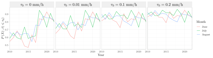
Figure S1.1: The temporal distribution of the proportion of observations, pooled in space, that are less than or equal to $\tau_{0}$ for June, July and August, respectively.

S2 Evaluation of fitted marginal distributions

We evaluate goodness of fit for the two marginal models by creating quantile-quantile (QQ) plots. It is not straightforward to compare empirical quantiles with our model quantiles, as the models assume that each day comes with a different distribution, and thus a different set of quantiles. To create QQ plots for the gamma model, we therefore standardise the data by dividing each observation on its estimated scale parameter. Then we compare empirical quantiles of the standardised data with quantiles from a gamma distribution with a scale parameter of 1 and the estimated shape parameter. The resulting QQ plots are displayed in the upper row of Figure S2.1. Similarly, to create QQ plots for the generalised Pareto (GP) model, we standardise the observed threshold exceedances by dividing on their estimated scale parameters, and then we compare empirical quantiles with those of a GP distribution with a scale of 1 and the estimated tail parameter. The QQ plots are displayed in the lower row of Figure S2.1. Both of the marginal models seem to perform well. The GP model slightly underestimates the largest quantiles, but we here note that a value of 10 mm/h is so large that it corresponds to the empirical $99.3\%$ quantile of the standardised threshold exceedances, which is approximately the same as the $99.97\%$ quantile of the nonzero precipitation observations, and approximately the same as the $1-5\times 10^{-5}$ quantile of the hourly summer precipitation observations, which again is slightly more than the 9 year return level for summer precipitation under the (unlikely) assumption that all observations are i.i.d.

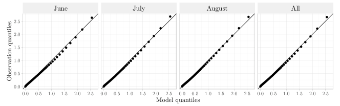
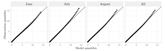
Figure S2.1: Upper row: QQ plots comparing empirical quantiles of the standardised observations with quantiles of a gamma distribution with a scale of 1 and the estimated shape parameter. Lower row: QQ plots comparing empirical quantiles of the standardised threshold exceedance observations with quantiles of a GP distribution with a scale of 1 and the estimated tail parameter. The four columns display empirical quantiles for June, July, August and for all the months together, respectively.

S3 Modelling the conditional intensity process

In the main paper, when modelling the conditional intensity process, we discover that the empirical estimators $\hat{\alpha}(d;y_{0})$ for $\alpha(d)$ seem to depend on $y_{0}$ for all values of $y_{0}$. We therefore propose to model $\alpha(\cdot)$ as a function $\alpha(d;y_{0})$ that depends on $y_{0}$, and we propose the form

$$\alpha(d;y_{0})=\exp\left[-{\left(d/\lambda_{a}(y_{0})\right)}^{\kappa_{a}(y_{0})}\right],$$

where $\lambda_{a}(y_{0}),\kappa_{a}(y_{0})>0$ are parametric functions of $y_{0}$.

Since the mean of our spatial conditional extremes model is $a(d;y_{0})=y_{0}\alpha(d;y_{0})$, we can easily estimate $\lambda_{a}(y_{0})$ and $\kappa_{a}(y_{0})$ for any fixed value of $y_{0}$, by minimising the sum of squared errors between $[Y(\bm{s})\mid Y(\bm{s}_{0})=y_{0}]$ and $a(\|\bm{s}-\bm{s}_{0}\|;y_{0})$. Thus, using a sliding window estimator over $y_{0}$, with a window size of $0.2$, we estimate $\lambda_{a}(y_{0})$ and $\kappa_{a}(y_{0})$ for a set of different threshold exceedances $y_{0}>\tau$. The estimators are displayed in the two leftmost plots of Figure S3.1. We see that the estimators for $\lambda_{a}(y_{0})$ seem to decay exponentially towards zero as $y_{0}$ increases, while the estimators for $\kappa_{a}(y_{0})$ look more like they follow the density function of a half-Gaussian distribution. We therefore propose the models

$$\lambda_{a}(y_{0})=\lambda_{a0}\exp(-(y_{0}-\tau)/\Lambda),\quad\kappa_{a}(y_{0})=\kappa_{a0}\exp(-{((y_{0}-\tau)/\Lambda_{\kappa})}^{\varkappa}),$$ (S3.1)

where the parameters $\lambda_{a0}$, $\Lambda$, $\kappa_{a0}$, $\Lambda_{\kappa}$ and $\varkappa$ all are required to be positive.

We fit the models in (S3.1) to the data by once more minimising the sum of squared errors. The resulting estimators for $\lambda_{a}(y_{0})$ and $\kappa_{a}(y_{0})$ are displayed as black lines in the two leftmost plots of Figure S3.1, and the resulting estimators for $\alpha(d;y_{0})$ and $a(d;y_{0})$ are displayed in the two rightmost plots of Figure S3.1. The fitted functions seem similar to those displayed in subplot A of Figure 3 in the main paper, and we therefore conclude that our chosen model for $\alpha(d;y_{0})$ provides an adequate fit to the data.

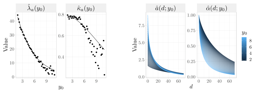
Figure S3.1: Leftmost plots: Points displaying least squares estimators of $\lambda_{a}(y_{0})$ and $\kappa_{a}(y_{0})$, computed using a sliding window over $y_{0}$ with a width of $0.2$. The black lines display the least squares estimators of $\lambda_{a}(y_{0})$ and $\kappa_{a}(y_{0})$ under the model in (S3.1), computed without the sliding window approach, i.e., using all possible threshold exceedances. Rightmost plots: The estimated functions for $\alpha(d;y_{0})$ and $a(d;y_{0})$, created using the least squares estimators of $\lambda_{a}(y_{0})$ and $\kappa_{a}(y_{0})$.

Having performed inference with R-INLA for the conditional intensity process using each of the five chosen conditioning sites, we evaluate model performance by simulating out-of-sample data and computing empirical estimators for $\mu(d;y_{0})$, $\zeta(d;y_{0})$, $\alpha(d)$, $\beta(d)$, $\sigma(d)$ and $\chi(d;y_{0})$, just as in Figure 3 in the main paper. Figure S4.1 displays these estimators for simulated data based on each of the five conditioning sites. It also displays the estimators from subplot A in Figure 3 of the main paper, which were computed “globally”, by using every single location $\mathcal{S}$ as a possible conditioning site. The estimators for $\beta(d)$ vary slightly between the different model fits, and this difference leads to considerable changes in the standard deviation $\zeta(d;y_{0})$ of the model fits. These differences might be caused by the fact that, as discussed in the main paper, our chosen model for $\beta(d)$ is somewhat simple, in that it does not account for the fact that the empirical estimators change as a function of $y_{0}$ for small values of $d$. Thus, for some model fits, $\beta(d)$ is given a value that captures the sharp spike of $\hat{\zeta}(d;y_{0})$ that occurs at small $d$ with large values of $y_{0}$, while for other fits, $\beta(d)$ is given a value that better captures the more smooth values of $\hat{\zeta}(d;y_{0})$ when $y_{0}$ is small. We believe that a more complex model for $\beta(d)$, possibly that changes as a function of $y_{0}$, would be able to capture both of these characteristics better. As shown in Section S4, the model fits with both of the different forms of $\beta(d)$ perform well and produce simulated data that closely capture important properties of the observed data such as its aggregated precipitation sums and extremal dependence structure.

S4 Evaluating the final precipitation simulations

We evaluate the precipitation simulations by computing conditional exceedance probability estimators and by creating QQ plots for the sums of aggregated precipitation over different areas inside the Stordalselva catchment. Figure S4.2 displays empirical estimators for $\chi_{p}(d)$ for both the observed and the simulated data, using each of the five conditioning sites. The simulated estimators correspond well to the observation estimators, overall. Yet, they tend to be smaller than those of the observed data for large $p$ and small $d$, and they tend to be larger than those of the observed data for small large $d$. This is further discussed in the main paper. Figure S4.3 display QQ plots for the sum of precipitation inside a ball of radius $d$, centred at $\bm{s}_{0}$, for each of the five conditioning sites, between the observed data and simulations from the four different model fits. The QQ plots show that there is a good correspondence between observed and simulated data, but that the simulated data tend to slightly underestimate aggregated precipitation amounts.

Figure S4.1: Estimators for $\mu(d;y_{0})$, $\zeta(d;y_{0})$, $\alpha(d)$, $\beta(d)$, $\sigma(d)$ and $\chi(d;y_{0})$ for observed data and for simulated data using the five chosen conditioning sites. The estimators are computed using the same sliding window approach as in the main paper.

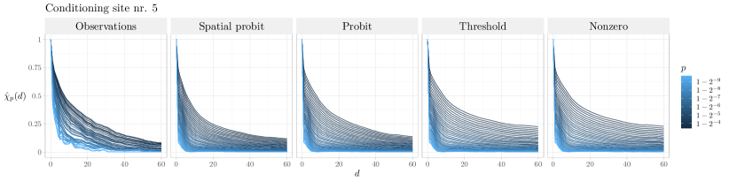
Figure S4.2: Estimators of $\chi_{p}(d)$ for observed and simulated data, using all five conditioning sites.

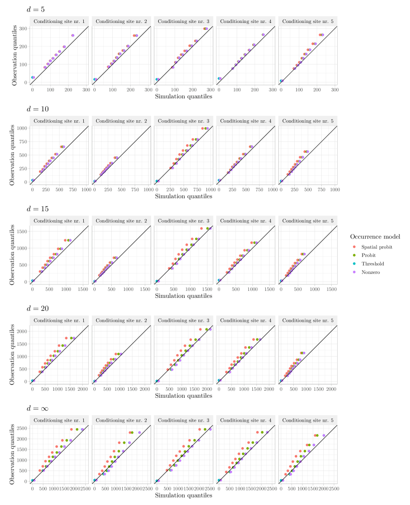
Figure S4.3: QQ plots for the sum of aggregated precipitation over the intersection of the Stordalselva catchment and a ball of radius $d$, centred at $\bm{s}_{0}$, for each of the five conditioning sites. The four different simulations are displayed using different colours.

References

- [1] Pierre Ailliot, Denis Allard, Valérie Monbet and Philippe Naveau “Stochastic Weather Generators: an Overview of Weather Type Models” In Journal de la Société Française de Statistique 156.1 Société française de statistique, 2015, pp. 101–113 URL: http://www.numdam.org/item/JSFS_2015__156_1_101_0/
- [2] Richard P. Allan et al. “Advances in Understanding Large-Scale Responses of the Water Cycle to Climate Change” In Annals of the New York Academy of Sciences 1472.1, 2020, pp. 49–75 DOI: 10.1111/nyas.14337
- [3] Jean-Noël Bacro, Carlo Gaetan, Thomas Opitz and Gwladys Toulemonde “Hierarchical Space-Time Modeling of Asymptotically Independent Exceedances With an Application to Precipitation Data” In Journal of the American Statistical Association 115.530 Taylor & Francis, 2020, pp. 555–569 DOI: 10.1080/01621459.2019.1617152
- [4] Sudipto Banerjee, Bradley P. Carlin and Alan E. Gelfand “Hierarchical Modeling and Analysis for Spatial Data”, Monographs on Statistics and Applied Probability Chapman & Hall/CRC, 2014 DOI: 10.1201/b17115
- [5] Günter Blöschl et al. “Current European Flood-Rich Period Exceptional Compared with Past 500 Years” In Nature 583.7817, 2020, pp. 560–566 DOI: 10.1038/s41586-020-2478-3
- [6] Apollon Bournas and Evangelos Baltas “Determination of the Z-R Relationship through Spatial Analysis of X-Band Weather Radar and Rain Gauge Data” In Hydrology 9.8, 2022 DOI: 10.3390/hydrology9080137
- [7] Rafael Cabral, David Bolin and Håvard Rue “Fitting latent non-Gaussian models using variational Bayes and Laplace approximations” arXiv, 2022 DOI: 10.48550/arxiv.2211.11050
- [8] Daniela Castro-Camilo, Raphaël Huser and Håvard Rue “A Spliced Gamma-Generalized Pareto Model for Short-Term Extreme Wind Speed Probabilistic Forecasting” In Journal of Agricultural, Biological and Environmental Statistics 24.3, 2019, pp. 517–534 DOI: 10.1007/s13253-019-00369-z
- [9] Daniela Castro-Camilo, Linda Mhalla and Thomas Opitz “Bayesian Space-Time Gap Filling for Inference on Extreme Hot-Spots: an Application to Red Sea Surface Temperatures” In Extremes 24.1, 2021, pp. 105–128 DOI: 10.1007/s10687-020-00394-z
- [10] Stefano Castruccio, Raphaël Huser and Marc G. Genton “High-Order Composite Likelihood Inference for Max-Stable Distributions and Processes” In Journal of Computational and Graphical Statistics 25.4 Taylor & Francis, 2016, pp. 1212–1229 DOI: 10.1080/10618600.2015.1086656
- [11] Daniel Cooley, Douglas Nychka and Philippe Naveau “Bayesian Spatial Modeling of Extreme Precipitation Return Levels” In Journal of the American Statistical Association 102.479 Taylor & Francis, 2007, pp. 824–840 DOI: 10.1198/016214506000000780
- [12] A.. Davison and R. Huser “Statistics of Extremes” In Annual Review of Statistics and Its Application 2.1, 2015, pp. 203–235 DOI: 10.1146/annurev-statistics-010814-020133
- [13] A.. Davison, S.. Padoan and M. Ribatet “Statistical Modeling of Spatial Extremes” In Statistical Science 27.2 The Institute of Mathematical Statistics, 2012, pp. 161–186 DOI: 10.1214/11-STS376
- [14] Anthony C. Davison, Raphaël Huser and Emeric Thibaud “Spatial Extremes” In Handbook of Environmental and Ecological Statistics ChapmanHall/CRC, 2019, pp. 711–744
- [15] Anita Verpe Dyrrdal, Alex Lenkoski, Thordis L. Thorarinsdottir and Frode Stordal “Bayesian Hierarchical Modeling of Extreme Hourly Precipitation in Norway” In Environmetrics 26.2, 2015, pp. 89–106 DOI: 10.1002/env.2301
- [16] Christoffer A. Elo “Correcting and Quantifying Radar Data” MET Norway report no. 2/2012, 2012
- [17] Sebastian Engelke, Thomas Opitz and Jennifer Wadsworth “Extremal Dependence of Random Scale Constructions” In Extremes 22.4, 2019, pp. 623–666 DOI: 10.1007/s10687-019-00353-3
- [18] Ludwig Fahrmeir, Thomas Kneib, Stefan Lang and Brian Marx “Regression” Springer, 2013 DOI: 10.1007/978-3-642-34333-9
- [19] Geir-Arne Fuglstad, Daniel Simpson, Finn Lindgren and Håvard Rue “Constructing Priors That Penalize the Complexity of Gaussian Random Fields” In Journal of the American Statistical Association 114.525 Taylor & Francis, 2019, pp. 445–452 DOI: 10.1080/01621459.2017.1415907
- [20] Alan E. Gelfand “Multivariate Spatial Process Models” In Handbook of Regional Science Berlin, Heidelberg: Springer Berlin Heidelberg, 2021, pp. 1985–2016 DOI: 10.1007/978-3-662-60723-7_120
- [21] Alan E. Gelfand, Peter J. Diggle, Montserrat Fuentes and Peter Guttorp “Handbook of Spatial Statistics” CRC press, 2010 DOI: 10.1201/9781420072884
- [22] Filippo Giorgi “Thirty Years of Regional Climate Modeling: Where Are We and Where Are We Going next?” In Journal of Geophysical Research: Atmospheres 124.11, 2019, pp. 5696–5723 DOI: 10.1029/2018JD030094
- [23] Inger Hanssen-Bauer et al. “Klima i Norge 2100” Kunnskapsgrunnlag for klimatilpasning oppdatert i 2015, Norsk klimasenter, Oslo, Norway, 2015
- [24] R. Huser and A.. Davison “Space-Time Modelling of Extreme Events” In Journal of the Royal Statistical Society: Series B (Statistical Methodology) 76.2, 2014, pp. 439–461 DOI: 10.1111/rssb.12035
- [25] Raphaël Huser and Jennifer L. Wadsworth “Modeling Spatial Processes With Unknown Extremal Dependence Class” In Journal of the American Statistical Association 114.525 Taylor & Francis, 2019, pp. 434–444 DOI: 10.1080/01621459.2017.1411813
- [26] Raphaël Huser and Jennifer L. Wadsworth “Advances in Statistical Modeling of Spatial Extremes” In Wiley Interdisciplinary Reviews (WIREs): Computational Statistics 14.1, 2022, pp. e1537 DOI: 10.1002/wics.1537
- [27] Raphaël Huser, Thomas Opitz and Emeric Thibaud “Bridging Asymptotic Independence and Dependence in Spatial Extremes using Gaussian Scale Mixtures” In Spatial Statistics 21, 2017, pp. 166–186 DOI: 10.1016/j.spasta.2017.06.004
- [28] Raphaël Huser, Thomas Opitz and Emeric Thibaud “Max-Infinitely Divisible Models and Inference for Spatial Extremes” In Scandinavian Journal of Statistics 48.1, 2021, pp. 321–348 DOI: 10.1111/sjos.12491
- [29] Harry Joe “Multivariate Models and Multivariate Dependence Concepts” ChapmanHall/CRC, 1997 DOI: 10.1201/9780367803896
- [30] Brenden Jongman “Effective Adaptation to Rising Flood Risk” In Nature Communications 9.1, 2018, pp. 1986 DOI: 10.1038/s41467-018-04396-1
- [31] Caroline Keef, Ioannis Papastathopoulos and Jonathan A. Tawn “Estimation of the Conditional Distribution of a Multivariate Variable Given That One of Its Components Is Large: Additional Constraints for the Heffernan and Tawn Model” In Journal of Multivariate Analysis 115, 2013, pp. 396–404 DOI: 10.1016/j.jmva.2012.10.012
- [32] Pavel Krupskii and Raphaël Huser “Modeling Spatial Tail Dependence with Cauchy Convolution Processes” In Electronic Journal of Statistics 16.2 Institute of Mathematical StatisticsBernoulli Society, 2022, pp. 6135–6174 DOI: 10.1214/22-EJS2081
- [33] Finn Lindgren and Håvard Rue “Bayesian Spatial Modelling with R-INLA” In Journal of Statistical Software 63.19, 2015, pp. 1–25 DOI: 10.18637/jss.v063.i19
- [34] Finn Lindgren, Håvard Rue and Johan Lindström “An Explicit Link Between Gaussian Fields and Gaussian Markov Random Fields: The Stochastic Partial Differential Equation Approach” In Journal of the Royal Statistical Society: Series B (Statistical Methodology) 73.4, 2011, pp. 423–498 DOI: 10.1111/j.1467-9868.2011.00777.x
- [35] Finn Lindgren et al. “A Diffusion-Based Spatio-Temporal Extension of Gaussian Matérn Fields”, 2023 DOI: 10.48550/arXiv.2006.04917
- [36] Tania Lopez-Cantu, Andreas F. Prein and Constantine Samaras “Uncertainties in Future U.S. Extreme Precipitation From Downscaled Climate Projections” In Geophysical Research Letters 47.9, 2020, pp. e2019GL086797 DOI: 10.1029/2019GL086797
- [37] Douglas Maraun and Martin Widmann “Statistical Downscaling and Bias Correction for Climate Research” Cambridge University Press, 2018 DOI: 10.1017/9781107588783
- [38] Roger B Nelsen “An Introduction to Copulas” Springer New York, 2006 DOI: 10.1007/0-387-28678-0
- [39] Thomas Opitz, Raphaël Huser, Haakon Bakka and Håvard Rue “INLA Goes Extreme: Bayesian Tail Regression for the Estimation of High Spatio-Temporal Quantiles” In Extremes 21.3, 2018, pp. 441–462 DOI: 10.1007/s10687-018-0324-x
- [40] S.. Padoan, M. Ribatet and S.. Sisson “Likelihood-Based Inference for Max-Stable Processes” In Journal of the American Statistical Association 105.489 Taylor & Francis, 2010, pp. 263–277 DOI: 10.1198/jasa.2009.tm08577
- [41] F. Palacios-Rodríguez, G. Toulemonde, J. Carreau and T. Opitz “Generalized Pareto Processes for Simulating Space-time Extreme Events: an Application to Precipitation Reanalyses” In Stochastic Environmental Research and Risk Assessment 34.12, 2020, pp. 2033–2052 DOI: 10.1007/s00477-020-01895-w
- [42] Simon Michael Papalexiou and Demetris Koutsoyiannis “Battle of Extreme Value Distributions: a Global Survey on Extreme Daily Rainfall” In Water Resour. Res. 49.1, 2013, pp. 187–201 DOI: 10.1029/2012WR012557
- [43] Jordan Richards, Jonathan A. Tawn and Simon Brown “Modelling Extremes of Spatial Aggregates of Precipitation using Conditional Methods” In The Annals of Applied Statistics 16.4 Institute of Mathematical Statistics, 2022, pp. 2693–2713 DOI: 10.1214/22-AOAS1609
- [44] Jordan Richards, Jonathan A. Tawn and Simon Brown “Joint estimation of Extreme Spatially Aggregated Precipitation at Different Scales through Mixture Modelling” In Spatial Statistics 53, 2023, pp. 100725 DOI: 10.1016/j.spasta.2022.100725
- [45] C.. Richardson “Stochastic Simulation of Daily Precipitation, Temperature, and Solar Radiation” In Water Resources Research 17.1, 1981, pp. 182–190 DOI: 10.1029/WR017i001p00182
- [46] Håvard Rue, Sara Martino and Nicolas Chopin “Approximate Bayesian Inference for Latent Gaussian Models By Using Integrated Nested Laplace Approximations” In Journal of the Royal Statistical Society: Series B (Statistical Methodology) 71.2, 2009, pp. 319–392 DOI: 10.1111/j.1467-9868.2008.00700.x
- [47] Rob Shooter et al. “Multivariate Spatial Conditional Extremes for Extreme Ocean Environments” In Ocean Engineering 247, 2022, pp. 110647 DOI: 10.1016/j.oceaneng.2022.110647
- [48] Daniel Simpson et al. “Penalising Model Component Complexity: a Principled, Practical Approach To Constructing Priors” In Statistical Science 32.1 The Institute of Mathematical Statistics, 2017, pp. 1–28 DOI: 10.1214/16-STS576
- [49] Emma S. Simpson and Jennifer L. Wadsworth “Conditional Modelling of Spatio-Temporal Extremes for Red Sea surface Temperatures” In Spatial Statistics 41, 2021, pp. 100482 DOI: 10.1016/j.spasta.2020.100482
- [50] Emma S. Simpson, Thomas Opitz and Jennifer L. Wadsworth “High-dimensional Modeling of Spatial and Spatio-Temporal Conditional Extremes using INLA and Gaussian Markov Random Fields” In Extremes, to appear arXiv, 2020 DOI: 10.48550/arxiv.2011.04486
- [51] H. Van de Vyver “Spatial Regression Models for Extreme Precipitation in Belgium” In Water Resources Research 48.9, 2012 DOI: 10.1029/2011WR011707
- [52] Silius M. Vandeskog, Sara Martino, Daniela Castro-Camilo and Håvard Rue “Modelling Sub-daily Precipitation Extremes with the Blended Generalised Extreme Value Distribution” In Journal of Agricultural, Biological and Environmental Statistics 27.4, 2022, pp. 598–621 DOI: 10.1007/s13253-022-00500-7
- [53] Silius M. Vandeskog, Sara Martino and Raphaël Huser “An Efficient Workflow for Modelling High-Dimensional Spatial Extremes” arXiv, 2022 DOI: 10.48550/arxiv.2210.00760
- [54] Silius M. Vandeskog, Sara Martino and Raphaël Huser “Supplement to “Fast Spatial Simulation of Extreme Precipitation from High-Resolution Radar Data Using INLA””, 2023
- [55] Janet Niekerk, Haakon Bakka, Håvard Rue and Olaf Schenk “New Frontiers in Bayesian Modeling Using the INLA Package in R” In Journal of Statistical Software 100.2, 2021, pp. 1–28 DOI: 10.18637/jss.v100.i02
- [56] Janet Niekerk, Elias Krainski, Denis Rustand and Håvard Rue “A New Avenue for Bayesian Inference with INLA” In Computational Statistics & Data Analysis 181, 2023, pp. 107692 DOI: 10.1016/j.csda.2023.107692
- [57] Andrew Verdin, Balaji Rajagopalan, William Kleiber and Richard W. Katz “Coupled Stochastic Weather Generation Using Spatial and Generalized Linear Models” In Stochastic Environmental Research and Risk Assessment 29.2, 2015, pp. 347–356 DOI: 10.1007/s00477-014-0911-6
- [58] Jennifer L. Wadsworth and Jonathan A. Tawn “Dependence Modelling for Spatial Extremes” In Biometrika 99.2, 2012, pp. 253–272 DOI: 10.1093/biomet/asr080
- [59] Jennifer L. Wadsworth and Jonathan A. Tawn “Higher-dimensional Spatial Extremes via Single-site Conditioning” In Spatial Statistics 51, 2022, pp. 100677 DOI: 10.1016/j.spasta.2022.100677
- [60] S. Westra et al. “Future Changes To the Intensity and Frequency of Short-Duration Extreme Rainfall” In Reviews of Geophysics 52.3, 2014, pp. 522–555 DOI: 10.1002/2014RG000464
- [61] Jiabo Yin et al. “Large Increase in Global Storm Runoff Rxtremes Driven by Climate and Anthropogenic Changes” In Nature Communications 9.1, 2018, pp. 4389 DOI: 10.1038/s41467-018-06765-2
- [62] Pierre Ailliot, Denis Allard, Valérie Monbet and Philippe Naveau “Stochastic Weather Generators: an Overview of Weather Type Models” In Journal de la Société Française de Statistique 156.1 Société française de statistique, 2015, pp. 101–113 URL: http://www.numdam.org/item/JSFS_2015__156_1_101_0/
- [63] Richard P. Allan et al. “Advances in Understanding Large-Scale Responses of the Water Cycle to Climate Change” In Annals of the New York Academy of Sciences 1472.1, 2020, pp. 49–75 DOI: 10.1111/nyas.14337
- [64] Jean-Noël Bacro, Carlo Gaetan, Thomas Opitz and Gwladys Toulemonde “Hierarchical Space-Time Modeling of Asymptotically Independent Exceedances With an Application to Precipitation Data” In Journal of the American Statistical Association 115.530 Taylor & Francis, 2020, pp. 555–569 DOI: 10.1080/01621459.2019.1617152
- [65] Sudipto Banerjee, Bradley P. Carlin and Alan E. Gelfand “Hierarchical Modeling and Analysis for Spatial Data”, Monographs on Statistics and Applied Probability Chapman & Hall/CRC, 2014 DOI: 10.1201/b17115
- [66] Günter Blöschl et al. “Current European Flood-Rich Period Exceptional Compared with Past 500 Years” In Nature 583.7817, 2020, pp. 560–566 DOI: 10.1038/s41586-020-2478-3
- [67] Apollon Bournas and Evangelos Baltas “Determination of the Z-R Relationship through Spatial Analysis of X-Band Weather Radar and Rain Gauge Data” In Hydrology 9.8, 2022 DOI: 10.3390/hydrology9080137
- [68] Rafael Cabral, David Bolin and Håvard Rue “Fitting latent non-Gaussian models using variational Bayes and Laplace approximations” arXiv, 2022 DOI: 10.48550/arxiv.2211.11050
- [69] Daniela Castro-Camilo, Raphaël Huser and Håvard Rue “A Spliced Gamma-Generalized Pareto Model for Short-Term Extreme Wind Speed Probabilistic Forecasting” In Journal of Agricultural, Biological and Environmental Statistics 24.3, 2019, pp. 517–534 DOI: 10.1007/s13253-019-00369-z
- [70] Daniela Castro-Camilo, Linda Mhalla and Thomas Opitz “Bayesian Space-Time Gap Filling for Inference on Extreme Hot-Spots: an Application to Red Sea Surface Temperatures” In Extremes 24.1, 2021, pp. 105–128 DOI: 10.1007/s10687-020-00394-z
- [71] Stefano Castruccio, Raphaël Huser and Marc G. Genton “High-Order Composite Likelihood Inference for Max-Stable Distributions and Processes” In Journal of Computational and Graphical Statistics 25.4 Taylor & Francis, 2016, pp. 1212–1229 DOI: 10.1080/10618600.2015.1086656
- [72] Daniel Cooley, Douglas Nychka and Philippe Naveau “Bayesian Spatial Modeling of Extreme Precipitation Return Levels” In Journal of the American Statistical Association 102.479 Taylor & Francis, 2007, pp. 824–840 DOI: 10.1198/016214506000000780
- [73] A.. Davison and R. Huser “Statistics of Extremes” In Annual Review of Statistics and Its Application 2.1, 2015, pp. 203–235 DOI: 10.1146/annurev-statistics-010814-020133
- [74] A.. Davison, S.. Padoan and M. Ribatet “Statistical Modeling of Spatial Extremes” In Statistical Science 27.2 The Institute of Mathematical Statistics, 2012, pp. 161–186 DOI: 10.1214/11-STS376
- [75] Anthony C. Davison, Raphaël Huser and Emeric Thibaud “Spatial Extremes” In Handbook of Environmental and Ecological Statistics ChapmanHall/CRC, 2019, pp. 711–744
- [76] Anita Verpe Dyrrdal, Alex Lenkoski, Thordis L. Thorarinsdottir and Frode Stordal “Bayesian Hierarchical Modeling of Extreme Hourly Precipitation in Norway” In Environmetrics 26.2, 2015, pp. 89–106 DOI: 10.1002/env.2301
- [77] Christoffer A. Elo “Correcting and Quantifying Radar Data” MET Norway report no. 2/2012, 2012
- [78] Sebastian Engelke, Thomas Opitz and Jennifer Wadsworth “Extremal Dependence of Random Scale Constructions” In Extremes 22.4, 2019, pp. 623–666 DOI: 10.1007/s10687-019-00353-3
- [79] Ludwig Fahrmeir, Thomas Kneib, Stefan Lang and Brian Marx “Regression” Springer, 2013 DOI: 10.1007/978-3-642-34333-9
- [80] Geir-Arne Fuglstad, Daniel Simpson, Finn Lindgren and Håvard Rue “Constructing Priors That Penalize the Complexity of Gaussian Random Fields” In Journal of the American Statistical Association 114.525 Taylor & Francis, 2019, pp. 445–452 DOI: 10.1080/01621459.2017.1415907
- [81] Alan E. Gelfand “Multivariate Spatial Process Models” In Handbook of Regional Science Berlin, Heidelberg: Springer Berlin Heidelberg, 2021, pp. 1985–2016 DOI: 10.1007/978-3-662-60723-7_120
- [82] Alan E. Gelfand, Peter J. Diggle, Montserrat Fuentes and Peter Guttorp “Handbook of Spatial Statistics” CRC press, 2010 DOI: 10.1201/9781420072884
- [83] Filippo Giorgi “Thirty Years of Regional Climate Modeling: Where Are We and Where Are We Going next?” In Journal of Geophysical Research: Atmospheres 124.11, 2019, pp. 5696–5723 DOI: 10.1029/2018JD030094
- [84] Inger Hanssen-Bauer et al. “Klima i Norge 2100” Kunnskapsgrunnlag for klimatilpasning oppdatert i 2015, Norsk klimasenter, Oslo, Norway, 2015
- [85] R. Huser and A.. Davison “Space-Time Modelling of Extreme Events” In Journal of the Royal Statistical Society: Series B (Statistical Methodology) 76.2, 2014, pp. 439–461 DOI: 10.1111/rssb.12035
- [86] Raphaël Huser, Thomas Opitz and Emeric Thibaud “Bridging Asymptotic Independence and Dependence in Spatial Extremes using Gaussian Scale Mixtures” In Spatial Statistics 21, 2017, pp. 166–186 DOI: 10.1016/j.spasta.2017.06.004
- [87] Raphaël Huser, Thomas Opitz and Emeric Thibaud “Max-Infinitely Divisible Models and Inference for Spatial Extremes” In Scandinavian Journal of Statistics 48.1, 2021, pp. 321–348 DOI: 10.1111/sjos.12491
- [88] Raphaël Huser and Jennifer L. Wadsworth “Modeling Spatial Processes With Unknown Extremal Dependence Class” In Journal of the American Statistical Association 114.525 Taylor & Francis, 2019, pp. 434–444 DOI: 10.1080/01621459.2017.1411813
- [89] Raphaël Huser and Jennifer L. Wadsworth “Advances in Statistical Modeling of Spatial Extremes” In Wiley Interdisciplinary Reviews (WIREs): Computational Statistics 14.1, 2022, pp. e1537 DOI: 10.1002/wics.1537
- [90] Harry Joe “Multivariate Models and Multivariate Dependence Concepts” ChapmanHall/CRC, 1997 DOI: 10.1201/9780367803896
- [91] Brenden Jongman “Effective Adaptation to Rising Flood Risk” In Nature Communications 9.1, 2018, pp. 1986 DOI: 10.1038/s41467-018-04396-1
- [92] Caroline Keef, Ioannis Papastathopoulos and Jonathan A. Tawn “Estimation of the Conditional Distribution of a Multivariate Variable Given That One of Its Components Is Large: Additional Constraints for the Heffernan and Tawn Model” In Journal of Multivariate Analysis 115, 2013, pp. 396–404 DOI: 10.1016/j.jmva.2012.10.012
- [93] Pavel Krupskii and Raphaël Huser “Modeling Spatial Tail Dependence with Cauchy Convolution Processes” In Electronic Journal of Statistics 16.2 Institute of Mathematical StatisticsBernoulli Society, 2022, pp. 6135–6174 DOI: 10.1214/22-EJS2081
- [94] Finn Lindgren et al. “A Diffusion-Based Spatio-Temporal Extension of Gaussian Matérn Fields”, 2023 DOI: 10.48550/arXiv.2006.04917
- [95] Finn Lindgren and Håvard Rue “Bayesian Spatial Modelling with R-INLA” In Journal of Statistical Software 63.19, 2015, pp. 1–25 DOI: 10.18637/jss.v063.i19
- [96] Finn Lindgren, Håvard Rue and Johan Lindström “An Explicit Link Between Gaussian Fields and Gaussian Markov Random Fields: The Stochastic Partial Differential Equation Approach” In Journal of the Royal Statistical Society: Series B (Statistical Methodology) 73.4, 2011, pp. 423–498 DOI: 10.1111/j.1467-9868.2011.00777.x
- [97] Tania Lopez-Cantu, Andreas F. Prein and Constantine Samaras “Uncertainties in Future U.S. Extreme Precipitation From Downscaled Climate Projections” In Geophysical Research Letters 47.9, 2020, pp. e2019GL086797 DOI: 10.1029/2019GL086797
- [98] Douglas Maraun and Martin Widmann “Statistical Downscaling and Bias Correction for Climate Research” Cambridge University Press, 2018 DOI: 10.1017/9781107588783
- [99] Roger B Nelsen “An Introduction to Copulas” Springer New York, 2006 DOI: 10.1007/0-387-28678-0
- [100] Thomas Opitz, Raphaël Huser, Haakon Bakka and Håvard Rue “INLA Goes Extreme: Bayesian Tail Regression for the Estimation of High Spatio-Temporal Quantiles” In Extremes 21.3, 2018, pp. 441–462 DOI: 10.1007/s10687-018-0324-x
- [101] S.. Padoan, M. Ribatet and S.. Sisson “Likelihood-Based Inference for Max-Stable Processes” In Journal of the American Statistical Association 105.489 Taylor & Francis, 2010, pp. 263–277 DOI: 10.1198/jasa.2009.tm08577
- [102] F. Palacios-Rodríguez, G. Toulemonde, J. Carreau and T. Opitz “Generalized Pareto Processes for Simulating Space-time Extreme Events: an Application to Precipitation Reanalyses” In Stochastic Environmental Research and Risk Assessment 34.12, 2020, pp. 2033–2052 DOI: 10.1007/s00477-020-01895-w
- [103] Simon Michael Papalexiou and Demetris Koutsoyiannis “Battle of Extreme Value Distributions: a Global Survey on Extreme Daily Rainfall” In Water Resour. Res. 49.1, 2013, pp. 187–201 DOI: 10.1029/2012WR012557
- [104] Jordan Richards, Jonathan A. Tawn and Simon Brown “Modelling Extremes of Spatial Aggregates of Precipitation using Conditional Methods” In The Annals of Applied Statistics 16.4 Institute of Mathematical Statistics, 2022, pp. 2693–2713 DOI: 10.1214/22-AOAS1609
- [105] Jordan Richards, Jonathan A. Tawn and Simon Brown “Joint estimation of Extreme Spatially Aggregated Precipitation at Different Scales through Mixture Modelling” In Spatial Statistics 53, 2023, pp. 100725 DOI: 10.1016/j.spasta.2022.100725
- [106] C.. Richardson “Stochastic Simulation of Daily Precipitation, Temperature, and Solar Radiation” In Water Resources Research 17.1, 1981, pp. 182–190 DOI: 10.1029/WR017i001p00182
- [107] Håvard Rue, Sara Martino and Nicolas Chopin “Approximate Bayesian Inference for Latent Gaussian Models By Using Integrated Nested Laplace Approximations” In Journal of the Royal Statistical Society: Series B (Statistical Methodology) 71.2, 2009, pp. 319–392 DOI: 10.1111/j.1467-9868.2008.00700.x
- [108] Rob Shooter et al. “Multivariate Spatial Conditional Extremes for Extreme Ocean Environments” In Ocean Engineering 247, 2022, pp. 110647 DOI: 10.1016/j.oceaneng.2022.110647
- [109] Daniel Simpson et al. “Penalising Model Component Complexity: a Principled, Practical Approach To Constructing Priors” In Statistical Science 32.1 The Institute of Mathematical Statistics, 2017, pp. 1–28 DOI: 10.1214/16-STS576
- [110] Emma S. Simpson, Thomas Opitz and Jennifer L. Wadsworth “High-dimensional Modeling of Spatial and Spatio-Temporal Conditional Extremes using INLA and Gaussian Markov Random Fields” In Extremes, to appear arXiv, 2020 DOI: 10.48550/arxiv.2011.04486
- [111] Emma S. Simpson and Jennifer L. Wadsworth “Conditional Modelling of Spatio-Temporal Extremes for Red Sea surface Temperatures” In Spatial Statistics 41, 2021, pp. 100482 DOI: 10.1016/j.spasta.2020.100482
- [112] H. Van de Vyver “Spatial Regression Models for Extreme Precipitation in Belgium” In Water Resources Research 48.9, 2012 DOI: 10.1029/2011WR011707
- [113] Silius M. Vandeskog, Sara Martino, Daniela Castro-Camilo and Håvard Rue “Modelling Sub-daily Precipitation Extremes with the Blended Generalised Extreme Value Distribution” In Journal of Agricultural, Biological and Environmental Statistics 27.4, 2022, pp. 598–621 DOI: 10.1007/s13253-022-00500-7
- [114] Silius M. Vandeskog, Sara Martino and Raphaël Huser “An Efficient Workflow for Modelling High-Dimensional Spatial Extremes” arXiv, 2022 DOI: 10.48550/arxiv.2210.00760
- [115] Silius M. Vandeskog, Sara Martino and Raphaël Huser “Supplement to “Fast Spatial Simulation of Extreme Precipitation from High-Resolution Radar Data Using INLA””, 2023
- [116] Janet Niekerk, Haakon Bakka, Håvard Rue and Olaf Schenk “New Frontiers in Bayesian Modeling Using the INLA Package in R” In Journal of Statistical Software 100.2, 2021, pp. 1–28 DOI: 10.18637/jss.v100.i02
- [117] Janet Niekerk, Elias Krainski, Denis Rustand and Håvard Rue “A New Avenue for Bayesian Inference with INLA” In Computational Statistics & Data Analysis 181, 2023, pp. 107692 DOI: 10.1016/j.csda.2023.107692
- [118] Andrew Verdin, Balaji Rajagopalan, William Kleiber and Richard W. Katz “Coupled Stochastic Weather Generation Using Spatial and Generalized Linear Models” In Stochastic Environmental Research and Risk Assessment 29.2, 2015, pp. 347–356 DOI: 10.1007/s00477-014-0911-6
- [119] Jennifer L. Wadsworth and Jonathan A. Tawn “Dependence Modelling for Spatial Extremes” In Biometrika 99.2, 2012, pp. 253–272 DOI: 10.1093/biomet/asr080
- [120] Jennifer L. Wadsworth and Jonathan A. Tawn “Higher-dimensional Spatial Extremes via Single-site Conditioning” In Spatial Statistics 51, 2022, pp. 100677 DOI: 10.1016/j.spasta.2022.100677
- [121] S. Westra et al. “Future Changes To the Intensity and Frequency of Short-Duration Extreme Rainfall” In Reviews of Geophysics 52.3, 2014, pp. 522–555 DOI: 10.1002/2014RG000464
- [122] Jiabo Yin et al. “Large Increase in Global Storm Runoff Rxtremes Driven by Climate and Anthropogenic Changes” In Nature Communications 9.1, 2018, pp. 4389 DOI: 10.1038/s41467-018-06765-2