Out-of-Order Sliding-Window Aggregation with
Efficient Bulk Evictions and Insertions (Extended Version)

Abstract.

Sliding-window aggregation is a foundational stream processing primitive that efficiently summarizes recent data. The state-of-the-art algorithms for sliding-window aggregation are highly efficient when stream data items are evicted or inserted one at a time, even when some of the insertions occur out-of-order. However, real-world streams are often not only out-of-order but also burtsy, causing data items to be evicted or inserted in larger bulks. This paper introduces a new algorithm for sliding-window aggregation with bulk eviction and bulk insertion. For the special case of single insert and evict, our algorithm matches the theoretical complexity of the best previous out-of-order algorithms. For the case of bulk evict, our algorithm improves upon the theoretical complexity of the best previous algorithm for that case and also outperforms it in practice. For the case of bulk insert, there are no prior algorithms, and our algorithm improves upon the naive approach of emulating bulk insert with a loop over single inserts, both in theory and in practice. Overall, this paper makes high-performance algorithms for sliding window aggregation more broadly applicable by efficiently handling the ubiquitous cases of out-of-order data and bursts.

PVLDB Artifact Availability:
The source code, data, and/or other artifacts have been made available at %leave␣empty␣if␣no␣availability␣url␣should␣be␣sethttps://github.com/IBM/sliding-window-aggregators.

1. Introduction

In data stream processing, a sliding window covers the most recent data, and sliding-window aggregation maintains a summary of it. Sliding-window aggregation is a foundational primitive for stream processing, and as such, is both widely used and widely supported. In various application domains, stream processing must have low latency; for example, late results can cause financial losses in trading or harm property and lives in security or transportation. Furthermore, streaming data often arrives out-of-order, but new data items must be incorporated into a sliding window at their correct timestamps and the aggregation may not be commutative. Finally, data streams do not always have a smooth rate: in the real world, data items often enter and depart sliding windows in bursts.

When streaming data is bursty, sliding-window aggregation needs to support efficient bulk evictions and insertions to keep latency low. In other words, it needs to evict or insert a bulk of $m$ data items faster than it would take to evict or insert them one by one, lest it incur a latency spike of $m\times$ that of a single operation. Bulk evictions are common in time-based windows, where the arrival of one data item at the youngest end of the window can trigger the eviction of several data items at the oldest end. For example, consider a window of size 60 seconds, with data items at timestamps [0.1,0.2,0.3,0.4,0.5,10,20,30,40,50,60] seconds. If the next data item to be inserted has timestamp 61, the window must evict the items at timestamps [0.1,0.2,0.3,0.4,0.5]. Since these are $m=5$ items, evicting them one by one would incur a $5\times$ latency spike.

While a small bulk (e.g., $m=5$) is harmless, bursts can result in $m$ in the thousands of data items or more. For instance, data streams may experience transient outages, causing bursts during recovery (Bouillet et al., 2012). Besides time-based windows, applications may use other window types such as sessions (Traub et al., 2019) or data-driven adaptive windows (Bifet and Gavaldà, 2007). Streaming systems may internally use implementation techniques that introduce disorder (Li et al., 2008). When a streaming system receives multiple streams from different data sources, their logical times may drift against each other (Krishnamurthy et al., 2010). Real-world events, such as breaking news, severe weather, rush hour traffic, sales, accidents, opening of stores or stock markets, etc. can cause bursty streams (Poppe et al., 2021). All these scenarios necessitate sliding-window aggregation with efficient bulk evictions and insertions—without harming the tuple-at-a-time performance.

The literature has few solutions to this problem, and none match our solution in completeness or algorithmic complexity. List-based approaches such as Two-Stacks handle neither out-of-order nor bulk operations (Tangwongsan et al., 2021). The AMTA algorithm only handles in-order windows and only offers bulk eviction but not bulk insertion (Villalba et al., 2019). CPiX has a linear factor in its algorithmic complexity for bulk eviction and is limited to commutative aggregation over time-based windows (Bou et al., 2021). The FiBA algorithm is optimal for out-of-order sliding-window aggregation with single evictions and insertions but does not directly support bulk operations (Tangwongsan et al., 2019). While the literature on balanced tree algorithms provides partial solutions to bulk evictions and insertions (Brown and Tarjan, 1979; Kaplan and Tarjan, 1995; Hinze and Paterson, 2006), each paper solves a different part of the problem using a different data structure, and none offer incremental aggregation. Section 2 discusses related work in more detail.

Our new solution builds on FiBA (Tangwongsan et al., 2019), a B-tree augmented with fingers and with location-sensitive partial aggregates. The fingers help efficiently find tree nodes to be manipulated when the window slides. The location-sensitive partial aggregates avoid propagating local updates to the root in most cases. Intuitively, our bulk eviction and insertion have three steps:

• a finger-based search to find the affected nodes of the tree;

• a single shared pass up the tree to insert or evict items in bulk while also repairing any imbalances this causes; and

• a single shared pass down the affected spine(s) of the tree to repair location-sensitive partial aggregates stored there.

The trick for efficient bulk evict is to not look at each evicted entry individually, but rather, only cut the tree along the boundary between the entries that go and those that stay. The trick for efficient bulk insert is to share work caused by multiple inserted entries as low down in the tree as possible, i.e., to process paths from insertion sites together as soon as they converge.

Let $n$ be the window size (the number of data items currently in the window); $m$, the bulk size (the number of data items being evicted or inserted); and $d$, the out-of-order insertion distance (the number of data items in the part of the window that overlaps with the bulk). Our algorithm performs bulk eviction in amortized $O(\log m)$ time and bulk insertion in amortized $O(m\log\frac{d}{m})$ time. Neither of these two time bounds depend on the window size $n$ and bulk eviction is sublinear in the bulk size $m$. For $m=1$, the amortized time matches the proven lower bounds of $O(1)$ for eviction and $O(\log d)$ for out-of-order insertion, which means $O(1)$ for in-order insertion at the smallest $d$. The worst-case time complexity is $O(\log n)$ for bulk evict and $O(m\log(\frac{m+n}{m})+\log d)$ for bulk insert, because the pass up the tree can reach the root in the worst case. This worst case is guaranteed to be so rare that in the long run, the amortized complexity prevails. It uses $O(n)$ space, with the constant depending on the B-tree’s arity.

We implemented our algorithm in C++ and made it available at https://github.com/IBM/sliding-window-aggregators, along with our implementations of other sliding-window aggregation algorithms we compare with experimentally. Commit f3beed2 was used in the experiments of this paper. Our experimental results demonstrate that our bulk evict yields the best latency compared to several state-of-the-art baselines, and our bulk insert yields the best latency for the out-of-order case (which most algorithms do not support at all in the first place). Overall, this paper presents the first algorithm for efficient bulk insertions in sliding windows, and the algorithm with the best time complexity so far for bulk evictions from sliding windows.

2. Related Work

Before our work, the most efficient algorithm for in-order sliding window aggregation with bulk eviction was AMTA (Villalba et al., 2019). AMTA supports single inserts or evicts in amortized $O(1)$ time. Given a window of size $n$, it supports bulk evict in amortized $O(\log n)$ time. However, AMTA does not directly support bulk insertion, so inserting $m$ items takes amortized $O(m)$ time. Our algorithm matches AMTA’s amortized complexity for single inserts and evicts, and improves bulk evict to amortized $O(\log m)$ time. Unlike our algorithm, AMTA does not support out-of-order insert.

CPiX supports both bulk eviction and bulk insertion, including out-of-order insertion (Bou et al., 2021). The paper states the time complexity of bulk insert or evict as $(p_{1}+1)\log(|\frac{n}{k}|)+3p_{2}$, where the number $k$ of checkpoints is recommended to be $\sqrt{n}$; $p_{1}$ is the number of affected partitions in the oldest checkpoint; and $p_{2}$ is the number of affected partitions in the remaining checkpoints. Given $O(\log(|\frac{n}{\sqrt{n}}|))=O(\log n)$, and assuming $p_{1}$ and $p_{2}$ are proportional to the batch size $m$, this corresponds to an amortized time of $O(m\log n)$. This is worse than AMTA’s $O(\log n)$ and our $O(\log m)$ for bulk evict. Moreover, unlike our algorithm, CPiX only works for time-based windows and commutative aggregation.

The most efficient prior algorithm for out-of-order sliding window aggregation is FiBA (Tangwongsan et al., 2019). It supports a single insert or evict in amortized $O(\log d)$ time, where $d$ is the distance of the operation from either end of the window. FiBA can emulate bulk insert or evict using loops of $m$ single inserts or evicts for a time complexity of $O(m\log d)$. Our new algorithm improves upon this baseline.

Some streaming systems limit out-of-order distance to a watermark (Akidau et al., 2013); instead, our algorithm implements the more general case that requires no such a priori bounds.

Our algorithm is inspired by the literature on bulk operations for balanced trees. Brown and Tarjan show how to merge two height-balanced trees of sizes $m$ and $n$, where $m<n$, in $O(m\log\frac{n}{m})$ steps (Brown and Tarjan, 1979). The keys of the two trees can be interspersed, so their algorithm corresponds to our out-of-order bulk insertion scenario. Unlike our algorithm, theirs supports neither aggregation nor bulk eviction. Furthermore, our algorithm improves the complexity to $O(m\log\frac{d}{m})$, where $d$ is the overlap between the two trees. Kaplan and Tarjan show how to catenate two height-balanced trees in worst-case $O(1)$ time (Kaplan and Tarjan, 1995). But they do not allow keys to be interspersed, so their approach is restricted to the in-order case. Also, unlike our algorithm, their approach does not perform aggregation and does not support bulk eviction. Hinze and Paterson show how to both split and merge balanced trees in amortized $O(\log d)$ time (Hinze and Paterson, 2006). However, their merge does not allow keys to be interspersed, so it corresponds to in-order bulk insertion. Also, their approach does not perform sliding window aggregation.

The sliding-window aggregation literature also pursues other objectives besides bulk eviction and out-of-order bulk insertion. Scotty optimizes for coarse-grained sliding, performing pre-aggregation to take advantage of co-eviction (Traub et al., 2019). Their work shows how to handle all combinations of order, window kinds, aggregation operations, etc., and is complementary to this paper. ChronicleDB uses a temporal aggregate B+-tree and optimizes writes to persistent storage while handling moderate amounts of out-of-order data by leaving some free space in each block (Seidemann et al., 2019). Hammer Slide uses SIMD instructions to speed up sliding-window aggregation (Theodorakis et al., 2018); SlideSide generalizes it to the multi-query case (Theodorakis et al., 2020b); and LightSaber further generalizes it for parallelism (Theodorakis et al., 2020a). DABA Lite performs both single in-order insert and single evict in worst-case $O(1)$ time but does not support out-of-order insert (Tangwongsan et al., 2021). FlatFIT focuses on window sharing for the in-order case, with amortized $O(1)$ time for single insert and single evict, but does not support out-of-order insert (Shein et al., 2017). None of the above directly support bulk operations; they can do $m$ inserts or evicts using simple loops, with an algorithmic complexity of $m$ times that of their single-operation complexity.

3. Background

This section formalizes the problem solved in this paper and reviews known concepts such as monoids and finger B-trees upon which our work builds.

3.1. Problem Statement

Monoids.

A monoid is a triple $(S,\otimes,\mathbf{1})$ with a set $S$, an associative binary combine operator $\otimes$, and a neutral element $\mathbf{1}$. Several common aggregation operators are monoids, including count, sum, min, and max. Furthermore, several more common aggregation operators can be lifted into monoids, including arithmetic or geometric mean, standard deviation, argMax, maxCount, first, last, etc. Even several sophisticated statistical and machine learning operators can be lifted into monoids, including mergeable sketches (Agarwal et al., 2012) such as Bloom filters or algebraic classifiers (Izbicki, 2013). Associativity means that $\forall v_{1},v_{2},v_{3}\in S:(v_{1}\otimes v_{2})\otimes v_{3}=v_{1}\otimes(v_{2}\otimes v_{3})$. That means we can omit the parentheses and simply write $v_{1}\otimes v_{2}\otimes v_{3}$; furthermore, in this paper, we sometimes even omit the $\otimes$ and simply use $v_{1}v_{2}v_{3}$ product notation. By giving flexibility over how values are grouped during combining, associativity is essential to most incremental sliding-window aggregation algorithms. The identity element $\mathbf{1}$ satisfies $\forall v\in S:\mathbf{1}\otimes v=v=v\otimes\mathbf{1}$. It gives meaning to aggregation over empty (sub)windows. For a monoid, while the combine operator $\otimes$ must be associative, it does not need to be invertible or commutative. Thus, any sliding-window aggregation algorithm that works for general monoids must handle the case of non-invertible and non-commutative operators.

Abstract Data Type.

Below we define an abstract data type with three operations query, bulkEvict, and bulkInsert. Our formulation decouples these three operations to make them as versatile as possible, so they can be used in any order, with any kind of window specification, including windows that grow and shrink dynamically. Of course, an abstract data type is not itself an algorithm; instead, it merely specifies the behavior that a given algorithm should implement. While it is easy to implement the abstract data type with a brute-force algorithm that recomputes everything from scratch, our problem statement is to design, analyze, and evaluate an incremental algorithm with native support for bulk operations that have better asymptotic and practical time complexity than before.

Query.

The operation query() makes no changes to the window and computes the monoidal combination of all values currently in the window in the order of their timestamps. Let the window contents be $W=\big{[}{t_{1}\atop v_{1}}\big{]},\ldots,\big{[}{t_{n}\atop v_{n}}\big{]}$ where $t_{i}<t_{i+1}$. Then query() returns $v_{1}\otimes\ldots\otimes v_{n}$, or the neutral element $\mathbf{1}$ if the window is empty.

Bulk Eviction.

The operation bulkEvict($t$) removes all entries with timestamps $\leq t$ from the window, leaving the entries with timestamps $>t$. Let the window contain $W^{\textrm{pre}}=\left\{\big{[}{t_{1}^{\textrm{pre}}\atop v_{1}^{\textrm{pre}}}\big{]},\ldots,\big{[}{t_{n}^{\textrm{pre}}\atop v_{n}^{\textrm{pre}}}\big{]}\right\}$ before eviction. Then, the window contents post-eviction are

$$W^{\textrm{post}}=\left\{\big{[}{t^{\textrm{post}}\atop v^{\textrm{post}}}\big{]}:\big{[}{t^{\textrm{post}}\atop v^{\textrm{post}}}\big{]}\in W^{\textrm{pre}}\wedge t^{\textrm{post}}>t\right\}.$$

Bulk Insertion.

The operation bulkInsert($B^{\textrm{in}}$), where the contents of the bulk to be inserted are $B^{\textrm{in}}=\left\{\big{[}{t_{1}^{\textrm{in}}\atop v_{1}^{\textrm{in}}}\big{]},\ldots,\big{[}{t_{m}^{\textrm{in}}\atop v_{m}^{\textrm{in}}}\big{]}\right\}$ with $t_{i}^{\textrm{in}}<t_{i+1}^{\textrm{in}}$, interleaves the previous window contents with the bulk in temporal order, and in case of collisions, combines them. Let the window contents pre-insertion be $W^{\textrm{pre}}=\left\{\big{[}{t_{1}^{\textrm{pre}}\atop v_{1}^{\textrm{pre}}}\big{]},\ldots,\big{[}{t_{n}^{\textrm{pre}}\atop v_{n}^{\textrm{pre}}}\big{]}\right\}$. Then, the window contents post-insertion are

$$\begin{array}[]{r@{\,}c@{\,}l}W^{\textrm{post}}&=&\left\{\big{[}{t^{\textrm{post}}\atop v^{\textrm{post}}}\big{]}:\big{[}{t^{\textrm{post}}\atop v^{\textrm{post}}}\big{]}\in W^{\textrm{pre}}\wedge\not\exists v^{\textrm{in}}:\big{[}{t^{\textrm{post}}\atop v^{\textrm{in}}}\big{]}\in B^{\textrm{in}}\right\}\\ &\cup&\left\{\big{[}{t^{\textrm{post}}\atop v^{\textrm{post}}}\big{]}:\big{[}{t^{\textrm{post}}\atop v^{\textrm{post}}}\big{]}\in B^{\textrm{in}}\wedge\not\exists v^{\textrm{pre}}:\big{[}{t^{\textrm{post}}\atop v^{\textrm{pre}}}\big{]}\in W^{\textrm{pre}}\right\}\\ &\cup&\left\{\big{[}{t^{\textrm{post}}\atop v^{\textrm{pre}}\otimes v^{\textrm{in}}}\big{]}:\big{[}{t^{\textrm{post}}\atop v^{\textrm{pre}}}\big{]}\in W^{\textrm{pre}}\wedge\big{[}{t^{\textrm{post}}\atop v^{\textrm{in}}}\big{]}\in B^{\textrm{in}}\right\}.\end{array}$$

3.2. FiBA Data Structure

Figure 1. FiBA data structure example.

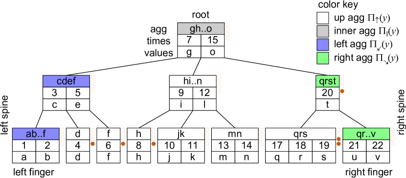
The FiBA data structure is a finger B-tree augmented for sliding-window aggregation. It was first introduced to optimize single out-of-order eviction and insertion (Tangwongsan et al., 2019). This paper uses the same data structure but introduces a new algorithm for bulk eviction and bulk insertion operations. Figure 1 gives a running example.

Node Contents.

Each node stores a partial aggregate agg and two parallel arrays of times and values $\big{[}{t_{i}\atop v_{i}}\big{]}$. For example, the aggregate of the second leaf from the right in Figure 1 is $\texttt{\small agg}=qrs$. Recall that $qrs$ is shorthand for $q\otimes r\otimes s$. While the data structure works with any monoid, assume for illustration that the monoid here is $\otimes=\max$ and that the values are $q=4$, $r=2$, and $s=5$. Then $\texttt{\small agg}=q\otimes r\otimes s=\max(4,2,5)=5$. In this example, timestamps are integers with almost no gaps, but there is a gap between times 15 and 17. In general, any totally ordered set will do for timestamps, and the data structure allows any number of gaps of any sizes.

Location-Sensitive Partial Aggregates.

At first glance, it would seem intuitive to set agg as the aggregation of a node and all its children and descendants. However, that would be suboptimal for sliding-window aggregation, because it would require propagating all window changes to the root, with time complexity $O(\log n)$. For a better time complexity, FiBA stores one of four different kinds of aggregate at each node depending on its location in the tree. Below are definitions of those four kinds of aggregates: up aggregate $\Pi_{\uparrow}$, inner aggregate $\Pi_{\hat{\scriptscriptstyle|}}$, left aggregate $\Pi_{\swarrow}$, and right aggregate $\Pi_{\searrow}$. In each of these definitions, let the current node under discussion be $y$ with arity $a$, children $c_{0},\ldots,c_{a-1}$, and values $v_{0},\ldots,v_{a-2}$.

• The up aggregate includes all children of $y$ and all of $y$’s own values in timestamp order:

  $$\Pi_{\uparrow}(y)=\Pi_{\uparrow}(c_{0})\otimes v_{0}\otimes\ldots\otimes v_{a-2}\otimes\Pi_{\uparrow}(c_{a-1})$$

  For example, the node with timestamps 9 and 12 in the middle of Figure 1 has $\texttt{\small agg}=hi..n$, which is the ordered monoidal combination starting from its left-most child, through all values and children, up to and including its right-most child. For a more concrete example, assume $h=4$, $i=5$, $j=1$, $k=3$, $l=5$, $m=4$, $n=2$ and the max monoid, then agg=5.

• The inner aggregate includes all of $y$’s own values and inner children but excludes the left-most and right-most child:

  $$\Pi_{\hat{\scriptscriptstyle|}}(y)=v_{0}\otimes\Pi_{\uparrow}(c_{1})\otimes\ldots\otimes\Pi_{\uparrow}(c_{a-2})\otimes v_{a-2}$$

  For example, the root in Figure 1 has $\texttt{\small agg}=gh..o$, which combines its left value $g$ with the aggregate of only the middle child $hi..n$ and the right value $o$. This means that the root stores an aggregate of the entire tree except for the left and right spines and their descendants.

• The left aggregate excludes the leftmost child but includes all of $y$’s own values and the rightmost child, and then combines that with the parent $x$ (unless $x$ is the root):

  $$\qquad\Pi_{\swarrow}(y)=\Pi_{\hat{\scriptscriptstyle|}}(y)\otimes\Pi_{\uparrow}(c_{a-1})\otimes\left(\begin{array}[]{ll}\mathbf{1}&\textrm{if }x\textrm{ is }\textit{root}\\ \Pi_{\swarrow}(x)&\textrm{otherwise}\end{array}\right)$$

  For example, the left-most leaf of Figure 1 has aggregate $\texttt{\small agg}=ab..f$, which combines its own values $ab$ with the aggregate $cdef$ of its parent, resulting in an aggregate of the entire left spine and all its descendants.

• The right aggregate combines the aggregate of the parent $x$ (unless $x$ is the root) with all of $y$’s own values and most children but excludes the rightmost child:

  $$\qquad\Pi_{\searrow}(y)=\left(\begin{array}[]{ll}\mathbf{1}&\textrm{if }x\textrm{ is }\textit{root}\\ \Pi_{\searrow}(x)&\textrm{otherwise}\end{array}\right)\otimes\Pi_{\uparrow}(c_{0})\otimes\Pi_{\hat{\scriptscriptstyle|}}(y)$$

  For example, the right-most leaf of Figure 1 has aggregate $\texttt{\small agg}=qr..v$, which combines the aggregate $qrst$ of its parent with its own values $uv$, resulting in an aggregate of the entire right spine and all its descendants.

Representation.

The tree is represented by three pointers: left finger to the left-most child; the root; and right finger to the right-most child. Each node stores its location-sensitive partial aggregate agg, times, and values, and in addition, has pointers to its parent and children, if any. Finally, each node stores two Boolean flags to indicate whether it is on the left or right spine, respectively.

Invariants.

The following properties about height, order, arity, and aggregates hold before each eviction or insertion and must be established again by the end of each eviction or insertion.

The height invariant requires all leaves to have the exact same distance from the root.

The order invariant says that the times $t_{0},\ldots,t_{a-2}$ within each node are ordered, i.e., $\forall i:t_{i}<t_{i+1}$; and furthermore, if a node has children $c_{0},\ldots,c_{a-1}$, then for all $i$, $t_{i}$ is greater than all times in $c_{i}$ or its descendants and smaller than all times in $c_{i+1}$ or its descendants.

The arity invariants constrain the sizes of nodes to keep the tree balanced. Each node has an arity $a$, and different nodes can have different arities. For non-leaf nodes, $a$ is the number of children. All nodes have $a-1$ entries, i.e., parallel arrays of $a-1$ timestamps and $a-1$ values. There is a data structure hyperparameter MIN_ARITY, which is an integer $>1$, and $\texttt{\small MAX\_ARITY}=2\cdot\texttt{\small MIN\_ARITY}$. They constrain the arity of all non-root nodes to $\texttt{\small MIN\_ARITY}\leq a\leq\texttt{\small MAX\_ARITY}$. And for the root, $2\leq a\leq\texttt{\small MAX\_ARITY}$. For example, MIN_ARITY is $2$ in Figure 1, so all non-leaf nodes have $2\leq a\leq 4$ children, and all nodes have $1\leq a-1\leq 3$ timestamps and values.

The aggregates invariants govern which nodes store which kind of location-sensitive aggregates, color-coded in Figure 1. All non-spine, non-root nodes store the up aggregate. Nodes that are on the left spine but not the root store the left aggregate. Nodes that are on the right spine but not the root store the right aggregate. And the root stores the inner aggregate. This means that the aggregate of the entire tree is simply the combination of the aggregates of the left finger, the root, and the right finger. In other words, we can implement query() in constant time by returning

$$\Pi_{\swarrow}(\texttt{\small leftFinger})\otimes\Pi_{\hat{\scriptscriptstyle|}}(\texttt{\small root})\otimes\Pi_{\searrow}(\texttt{\small rightFinger})$$

Imaginary Coins.

To help prove the amortized time complexity, we pretend that each node stores imaginary coins. Figure 1 shows these as small copper circles. Nodes that are close to underflowing store one coin to pay for the rebalancing work in case of underflow. Nodes that are close to overflowing store two coins to pay for the rebalancing work in case of overflow. Then, the proofs for amortized time complexity show that for any possible sequence of operations, the algorithm always stores up enough coins in advance at each node before it has to perform eventual actual rebalancing work.

4. Bulk Eviction

As defined in Section 3.1, bulkEvict($t$) removes all entries with timestamps $\leq t$ from the window. So our algorithm must discard nodes to the left of $t$, keep nodes to the right of $t$, and for nodes that straddle the boundary, locally evict all entries up to $t$ and repair any violated invariants. Our bulk eviction algorithm has three steps:

1. A finger-based eviction boundary search that returns a list, called boundary, of triples (node, ancestor, neighbor).

2. A pass up the boundary, and beyond as needed to repair invariants, that does the actual evictions and most repairs.

3. A pass down the left spine, and if needed also the right spine, that repairs any leftover invariant violations.

Bulk eviction Step 1: Eviction boundary search. This step finds the boundary to enable any subsequent rebalancing operations during Step 2 to be constant-time at each level. For rebalancing to be efficient, it cannot afford to trigger any searches of its own, and must instead rely on all required searching to have already been done upfront. Whereas textbook algorithms for B-trees with single evictions (such as (Cormen et al., 1990)) can repair arity invariants by rebalancing with a node’s left or right sibling, bulk eviction leaves no left sibling. That means the only eligible neighbor to help in rebalancing is the right one, and that may have a different parent and thus not be a sibling. Furthermore, rebalancing requires the least common ancestor of the node and its neighbor, and that might not be their parent. Hence, the job of the finger-based search is to find a list of (node, ancestor, neighbor) triples, one for each relevant level of the tree. The search first starts at the left or right finger, whichever is closest to $t$, and walks up the corresponding spine to find the top of the boundary, i.e., the lowest spine node whose descendants straddle $t$. Then, the search traverses down to the actual eviction point while populating the boundary data structure. This downward traversal always keeps at most two separate chains for the node and its neighbor, and can thus happen in a single loop over descending tree levels. If the search finds an exact match for $t$ in the tree, it stops early; otherwise, it continues to a leaf and stops there.

Bulk eviction Step 2: Pass up. This step of the algorithm does most of the work: it performs the actual evictions, and along the way, it also repairs most of the invariants that those evictions may have violated. Recall from Section 3.2 that there are invariants about height, order, arity, and location-sensitive partial aggregates. The pass up never violates invariants about height or order. It immediately restores arity invariants, using some novel rebalancing techniques described below. Regarding aggregate invariants, the pass up only repairs aggregates that follow a strictly ascending direction (up aggregates $\Pi_{\uparrow}$ and inner aggregates $\Pi_{\hat{\scriptscriptstyle|}}$). The pass up leaves aggregates that involve the parent (left aggregates $\Pi_{\swarrow}$ and right aggregates $\Pi_{\searrow}$) to the later pass down to repair.

The pass up has two phases: an eviction loop up the boundary returned by the search, followed by a repair loop further up beyond the boundary as long as there is more to repair. At each level, the eviction loop performs the local eviction, repairs arity underflow, and repairs local up aggregates or inner aggregates. At each level that still needs such repair, the repair loop repairs arity underflow and repairs local up aggregates or inner aggregates. Aggregate repair happens in constant time per level by simply recomputing aggregates of surviving affected nodes after eviction and rebalancing are done. Arity repair, also known as rebalancing, either moves entries from the neighbor to the node or merges the node into the neighbor, depending on their respective arities. Let nodeDeficit be $\texttt{\small MIN\_ARITY}-\texttt{\small node.arity}$ and let neighborSurplus be $\texttt{\small neighbor.arity}-\texttt{\small MIN\_ARITY}$. If $\texttt{\small nodeDeficit}\leq\texttt{\small neighborSurplus}$, rebalancing does a move; otherwise, it does a merge.

Figure 2. Move batch.

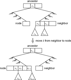
Figure 2 illustrates the move operation, representing each pair $\big{[}{t_{x}\atop v_{x}}\big{]}$ of timestamp and value as an entry $e_{x}$. In this figure, $k$ corresponds to nodeDeficit, i.e., the number of entries and children to move to node to repair its underflow by bringing its arity back to MIN_ARITY. In contrast to the textbook move operation (Cormen et al., 1990), $k$ may exceed 1 and neighbor may not be a sibling of node. The only entry of the ordered window that is between node and neighbor is $e_{a}$ in their least common ancestor. So the move rotates $e_{a}$ into node, along with $e_{0},\ldots,e_{k-2}$ and all associated children, and rotates $e_{k-1}$ to the ancestor. In the end, node has arity MIN_ARITY and neighbor has arity $\geq\texttt{\small MIN\_ARITY}$, because it started with sufficient surplus. Of course, neighbor still has arity $\leq\texttt{\small MAX\_ARITY}$, because it started out that way and did not grow any bigger. Figure LABEL:fig:move_batch_example shows pseudocode and a concrete example for move.

Figure 3. Merge with neighbor (non-sibling).

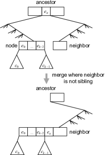
Figure 3 illustrates merge, which adds what is left of node to neighbor and then eliminates node. Unlike in the textbook B-tree setup, node and neighbor may not be direct siblings. Since any other vertices on the path from node to ancestor are entirely $<t$, those vertices will also be eliminated. On the other hand, $e_{a}$ has a timestamp $>t$, so it remains in the tree, and we rotate it into neighbor. Let oldNodeArity and oldNeighborArity refer to the arity of the node and its neighbor before the merge. Then, after the merge, we have

$$\begin{array}[]{l@{\,}l@{\,}l}&\texttt{\small neighbor.arity}\\ ={}&\texttt{\small oldNodeArity}&+\,\texttt{\small oldNeighborArity}\\ ={}&\texttt{\small MIN\_ARITY}-\texttt{\small nodeDeficit}&+\,\texttt{\small MIN\_ARITY}+\texttt{\small neighborSurplus}\\ ={}&\,\lx@intercol 2\cdot\texttt{\small MIN\_ARITY}+(\texttt{\small neighborSurplus}-\texttt{\small nodeDeficit})\hfil\lx@intercol\\ \end{array}$$

This means that there is no overflow, because merge only happens when $\texttt{\small nodeDeficit}>\texttt{\small neighborSurplus}$, and there is no underflow, because $\texttt{\small nodeDeficit}\leq\texttt{\small MIN\_ARITY}$ and $\texttt{\small neighborSurplus}\geq 0$. See code and example in Figure LABEL:fig:merge_notsibling_example.

Figure 4. Make node root.

Figure 5. Make child root.

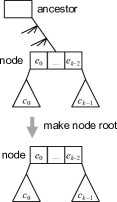
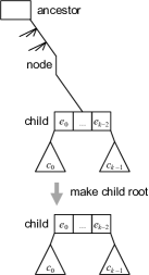
For bulkEvict($t$) to be fully general, it must handle the case where $t$ is all the way on the right spine. This implies that the root itself is to the left of $t$ and must be eliminated. Eliminating the root shrinks the tree from the top, thus preserving the height invariant, and requires giving the tree a new root lower down. There are two sub-cases for shrinking the tree given a node on the right spine. If, after the local eviction, the node still has arity $>1$, the algorithm makes it the root (Figure 5); otherwise, the node has arity $=1$ and the algorithm makes its single child the root (Figure 5). Figure LABEL:fig:make_child_root_example shows pseudocode and an example.

Bulk eviction Step 3: Pass down. The last step of the algorithm repairs left aggregates and spine flags on the left spine. In case the eviction touched the right spine, it also repairs right aggregates and spine flags on the right spine. Recall that the left aggregate and right aggregate of a node are computed using the aggregate result from its parent. Hence, the pass down loops over tree levels and performs a local recompute to propagate these changes.

Theorem 1.

The algorithm for bulkEvict($t$) takes $O(\log m)$ amortized time and $O(\log n)$ worst-case time.

Proof.

Consider the steps of the algorithm separately. Step 1, the finger-based search, takes time $O(\log m)$ worst-case, since it takes a single traversal up from a finger to the lowest ancestor containing $t$ followed by a single traversal down at most to a leaf. Step 2, the pass up, comprises an eviction loop followed by a repair loop. The eviction loop takes time $O(\log m)$ worst-case, since it traverses the boundary list returned by the search. The repair loop might continue to repair overflow past the top of the boundary. In the worst case, it might reach the root, bringing the total time complexity of the evict loop plus repair loop to $O(\log n)$ worst-case. However, since the repair loop starts above the boundary, at its start, it can at most have to deal with an underflow of a single entry. Therefore, it meets the conditions of Lemma 9 from the FiBA paper (Tangwongsan et al., 2019), which uses virtual coins to show that the amortized cost for the repair loop is $O(1)$. This brings the total amortized time of the pass up to $O(\log m+1)=O(\log m)$. Finally, Step 3, the pass down, traverses the same number of levels as the pass up. ∎

5. Bulk Insertion

As defined in Section 3.1, bulkInsert($B^{\textrm{in}}$) inserts one or more entries into the window. The bulk of entries is modeled as an iterator of (timestamp, value) pairs, which are assumed to be timestamp-ordered. Our bulkInsert algorithm processes the bulk in three steps:

1. A finger-based insertion sites search that, without making any modifications, locates all the sites in the tree where new entries need to be inserted.

2. A pass up: interleave&split loop that, starting at the leaves, interleaves the new entries into their respective nodes, splitting the node and promoting keys as necessary to satisfy the arity invariants. This happens from the leaves up until no level requires further processing.

3. A pass down the right spine, and if needed also the left spine, that repairs any leftover aggregation invariant violations.

The remainder of this section delves deeper into the details of these steps and their cost analysis. Later, Section 6 discusses their implementation and optimization maneuvers.

Bulk insertion Step 1: Insertion sites search. To locate the insertion sites, the algorithm conducts the search in timestamp order, beginning with the earliest timestamp in the bulk using finger search. Each subsequent search never has to go higher than the least common ancestor between the previous node and its insertion site. This step associates each (timestamp, value) pair from the input with the corresponding node into which it will be inserted.

Like in a standard B-tree structure, each new timestamp (key) that is not yet in the tree will be inserted at a leaf location. Such a key can cause cascading changes to the tree structure and, in the context of FiBA, can additionally trigger a chain of recomputation of aggregation values starting from the insertion site. On the other hand, a timestamp that is already in the tree is destined to the node where that timestamp is present, where the aggregation monoid combines its value with the existing value. This results in no structural changes, but in the context of FiBA, this triggers a chain of recomputation of aggregation values starting from that node. We see both cases as events that require processing: an insertion event adds a real entry to the target node and recomputes the aggregation value, whereas a recomputation event merely indicates the node where recomputation must take place.

$\rhd$ Treelets. Concretely, the implementation represents each event as a treelet tuple (target, timestamp, value, childNode, kind). This indicates that this particular (timestamp, value) pair with a child childNode (possibly NULL) is to be inserted into the target node unless the kind is a recomputation event, in which case it simply triggers a recomputation of aggregate values on the target node. Treelets form the backbone of the bulkInsert logic, with Step 1 (the insertion sites search) creating the initial timestamp-ordered sequence of treelets targeting all the relevant insertion sites.

Figure 6. Interleave and split for one level of a tree

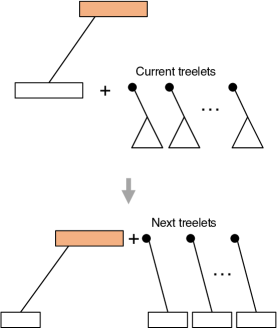
Bulk insertion Step 2: Pass up: interleave&split loop. As the next step, the algorithm proceeds level by level, working its way from the leaf level towards the root until no more changes happen. At any point, the algorithm aims to maintain only two levels of treelets—the current level and the next level. In this view, as illustrated in Figure 6, each level takes as input a sequence of treelets and produces a sequence of treelets for the next level. Since the treelets in the input are timestamp-ordered, the entries destined for the same node appear consecutively in the sequence and are easily identified. Conceptually, each level is processed as follows:

For each target $t$ in the input sequence of treelets:

1. Gather all the treelets that target $t$ into TL.

2. Interleave the contents of $t$ with TL. Since both of these are ordered, the interleave routine is the merge step of the well-known merge-sort algorithm. Interleaving takes time linear in the total length of its input sequences to produce an ordered output sequence without requiring a separate sort step.

3. If $t$ has arity more than MAX_ARITY, apply bulkSplit to split it into smaller nodes.

When multiple entries are added to the same node, a node can temporarily overflow to arity $p>\texttt{\small MAX_ARITY}=2\mu$, often $p\gg 2\mu$. The bulkSplit routine then splits it into invariant-respecting nodes, consisting of one or more arity-$(\mu+1)$ nodes and one last node with arity between $\mu$ and $2\mu$. The following claim, which is intuitive and whose proof appears in the appendix, shows that it is possible to split such a node into legitimate FiBA nodes in this way:

Claim 1.

Let $p>\texttt{\small MAX_ARITY}~{}=2\mu$ be an integral temporary arity. The number $p$ can be written as

$$p=b_{0}+b_{1}+\dots+b_{t-1}+b_{t},$$

where $b_{0}=b_{1}=\dots b_{t-1}=\mu+1$ and $\mu\leq b_{t}\leq 2\mu$.

For example, if $p=2\mu+3$ with $\mu=4$, we can write $p$ as $p=(\mu+1)+(\mu+2)$. That is, this split yields one arity-$(\mu+1)$ node, one entry to send up to the next level, and one arity-$(\mu+2)$ node. If $p=7\mu+2$ with $\mu=2$, we can write $p$ as $p=\mu+1+\mu+1+\mu+1+\mu+1+2\mu$. That is, this split yields four arity-$(\mu+1)$ nodes and one arity-$2\mu$ node, interspersed with $4$ entries to send up to the next level.

$\rhd$ Promotion to the next level. Splitting an overflowed node also generates treelets, representing entries promoted for insertion into nodes in the next level. Importantly, by processing current-level treelets in timestamp order, new treelets for the next level generated in this manner are already sorted in timestamp order. This helps avoid the costly step of sorting them or the need for a priority queue. Additionally, the parent of each existing node is the target insertion site of the corresponding promoted entry.

The discussion so far left out recomputation events. There are two ways a recomputation event is created: (a) inserting an entry with an existing timestamp and (b) incorporating entries into a node without causing it to overflow. Case (a) happens in Step 1 (insertion sites search) but can target nodes anywhere in the tree, not just the leaves. Case (b) happens throughout Step 2 (making a pass up). Because of how Step 1 is carried out and to sidestep the need to store treelets for future levels and interleave in treelets for recomputation events when their levels are reached, we start all the recomputation events/treelets at the leaf level. These treelets will ride along with the other treelets but will not have a real effect until their levels are reached. This turns out to have the same asymptotic complexity as if we were to start them at their true levels—but without the additional code complexity.

Bulk insertion Step 3: Pass down. Like in the bulkEvict algorithm, the final step repairs right aggregates on the right spine and potentially left aggregates on the left spine if it also touches the left spine. For both spines, the aggregate of a node is computed using the value from its parent, so this computation is a pass on the spine towards the finger (i.e., rightmost and leftmost leaf).

Bulk insertion: Time complexity analysis. The time complexity of bulkInsert can be broken down into (i) the search cost (Step 1), (ii) insertion and tree restructuring (Step 2), and (iii) aggregation repairs (during Steps 2 and 3). To analyze this, we begin by proving a lemma that quantifies the footprint—the worst-case number of nodes that can be affected—when there are $m$ insertion sites.

For a bulkInsert call, the top node, denoted by $\tau$, is the least-common ancestor of all insertion sites and the rightmost finger. By definition, this is the node closest to the leaf level where paths from all these sites towards the root converge.

Lemma 1.

In a FiBA structure with MAX_ARITY$\,=2\mu$, if there are $m$ insertion sites, the paths from all the insertion sites, as well as the node at the right finger, to the top $\tau$ contain at most $O(m(1+\log_{2\mu}(\tfrac{N_{\tau}}{m})))$ unique nodes, where $N_{\tau}$ is the total number of nodes in the subtree rooted at $\tau$.

Proof.

Consider the subtree rooted at the top node $\tau$. For level $\ell=0,1,\dots$ away from the top, the total number of nodes at that level $n_{\ell}$ satisfies

(1) $$\mu^{\ell}\leq n_{\ell}\leq(2\mu)^{\ell},$$

which holds because the fan-out degree for non-root nodes is between $\mu$ and $2\mu$ (inclusive). Now we will assume all the insertion sites are at the leaf level. This can be arranged by projecting every insertion site onto a leaf within its own subtree, and doing so can only increase the number of nodes contributing to the bound.

By (1), the leaves must be at level $L\leq\log_{\mu}N_{\tau}$ and the smallest level $\ell$ that has no more than $m$ nodes is $\ell\geq\log_{2\mu}m$. This means the paths from the leaf insertion sites can travel without necessarily converging together for $L-\ell$ levels. During this stretch, the number of unique nodes is at most $m(L-\ell)=O(m\log_{2\mu}(N_{\tau}/m))$. From level $\ell$ to the top node, the paths must converge as constrained by the shape of the tree. In a B-tree with $m$ leaves, the number of nodes at each level decreases geometrically towards the top. Hence, there are at most $O(m)$ unique nodes from levels $\ell$ and above, for a grand total of $O(m(1+\log_{2\mu}(\tfrac{N_{\tau}}{m})))$ unique nodes. ∎

Next, we address the tree restructuring cost:

Lemma 2.

Let $\mu\geq 2$. The tree restructuring cost of inserting $m$ entries in a bulk is amortized $O(m)$ and worst-case $O(m\log(\frac{m+n}{m}))$, where $n$ is the number of entries prior to the bulk insertion operation.

The worst-case bound can be easily seen: the $m$ insertions can only change the nodes from $m$ leaves to the root, touching at most $O(m\log(\frac{m+n}{m}))$ nodes (Lemma 1). For the amortized bound, the proof is analogous to Lemma 9 in the FiBA paper (Tangwongsan et al., 2019), arguing that charging $2$ coins per new entry is sufficient in maintaining the tree. More details appear in the appendix.

Theorem 3.

The algorithm for bulkInsert runs in amortized $O(\log d+m(1+\log(\tfrac{d}{m})))$ time and $O(\log d+m\log(\frac{m+n}{m}))$ worst-case time, where $m$ is the number of entries in the bulk and $d$ is the out-of-order distance of the earliest entry in the bulk.

Proof.

The running time of bulkInsert is made up of (i) the search cost (Step 1), (ii) insertion and tree restructuring (Step 2), and (iii) aggregation repairs (during Steps 2 and 3).

The first search for the insertion site takes $O(\log d)$, thanks to finger searching from the right finger. Each subsequent search only traverses the path from the previous entry to their least common ancestor and down to the next entry. The whole search cost is therefore covered by Lemma 1. After that, the actual insertion takes $O(1)$ time per entry since interleaving takes time that is linear in its input. The cost to further restructure the tree is as described in Lemma 2. Finally, it is easy to see that the cost of aggregation recomputation/repairs is subsumed by the first two costs because the aggregation of a node has to be recomputed only if it was part of the restructuring or sits on the search path (spine or on the way to the top node). Adding up the costs yields the stated bounds. ∎

This means asymptotically bulkInsert is never more expensive than individually inserting entries. On the contrary, bulk insertion results in cost savings as insertion-site search and restructuring work can be shared.

6. Implementation

We implemented our algorithm in C++ because of its strong and predictable raw performance in terms of both time and space. Using C++ avoids latency spikes from runtime services, such as garbage collection or just-in-time compilation, common in managed languages such as Java or Python. Such extraneous latency spikes would obscure the latency effects of our algorithm. The results section contains apples-to-apples comparisons with other sliding-window aggregation algorithms from prior work that was also implemented in C++. We reuse code between our new algorithm and those earlier algorithms. In particular, we use C++ templates to specialize each algorithm for each given aggregation monoid, and share the same implementation of the aggregation monoids across all algorithms. The C++ compiler then inlines both the monoid’s data structure and its operator code into the sliding-window aggregation data structure and algorithm code as appropriate.

Deferred free list. Our implementation has to avoid reclaiming memory eagerly. If bulk eviction reclaimed memory eagerly, the promised algorithmic complexity would be spoiled: Given that the arity of the tree is controlled by a constant hyperparameter MIN_ARITY, eagerly evicting a bulk of $m$ entries would require reclaiming the memory of $O(m)$ nodes. Those $O(m)$ calls to delete would be worse than the amortized complexity of $O(\log m)$ for bulk evict. Therefore, we avoid eager memory reclamation as follows: Recall that the eviction loop iterates over $O(\log m)$ nodes on the boundary and, for each node, performs local evictions, which will proceed to evict the children of that node. Instead of recursively deleting all the descendants eagerly, the local evict places their children on a deferred free-list. Since at most $O(\log m)$ nodes can be removed, the cost of adding only the children to the free list during bulk eviction is worst-case $O(\log m)$. Later, when an insertion would require a new allocation, it first checks the free-list. If that is non-empty, it pops one node, pushes its children, and reuses its memory for the new node. Thus, each insert only spends worst-case $O(1)$ time on memory reuse.

Memory mangement during bulkInsert. Conceptually, we allow a node to grow to an arbitrary size before splitting it into invariant-respecting smaller nodes. For performance, the implementation does this differently. The main goal is to minimize memory allocation and deallocation for intermediate storage. To combine keys from an existing node with keys to be inserted into that node, it employs an ordered interleaving routine from merge sort. Here the interleaving is lazy: instead of generating the combined sequence of keys upfront, our implementation offers an iterator for the interleaved sequence that computes the next element on the fly, reading directly from two sources—the existing node and the sequence of treelets for the current level. We also have an optimization where if the node is not going to overflow after incorporating the new keys (“small insertion”), then simple insertion is used as there would be no memory allocation involved.

Additional optimization includes (i) using alternating buffers for treelet processing and (ii) consolidating treelets. For treelet processing, the dataflow pattern is reading from the current level and writing to the next level. Each sequence is progressively smaller as the algorithm works its way up the tree. Hence, we allocate two vectors with enough capacity at the start and alternate between them as the algorithm proceeds. Furthermore, treelets that will be inserted into the same node are consolidated together. This reduces the struct size because the target node does not need to be repeated for each of these treelets.

Miscellanea. As described, our algorithm already combines entries with the same timestamp at insert, thus reducing memory. Users can choose to coarsen the granularity of timestamps, thus causing more cases of equal timestamps, recovering basic batching. However, it would require additional work to take full advantage of batching, such as for energy efficiency (Michalke et al., 2021). Our implementation does not directly use SIMD instructions, but the C++ optimizing compiler sometimes uses them automatically. We did not implement partitioning but it is straightforward: when the aggregate is partitioned by key, keep disjoint state, i.e., a separate tree for each key; that would enable fission (Hirzel et al., 2017) for parallelization, either user-directed or automatically. Previous work describes an algorithm for range queries (Tangwongsan et al., 2019), and that algorithm also works in the presence of bulk insertion and eviction. Future work could pursue a new algorithm for multi-range queries.

Figure 7. Latency, bulk evict only, window size $n=\textrm{4,194,304}$, bulk size $m=\textrm{1,024}$, in-order data $d=\textrm{0}$.

Figure 8. Latency, bulk insert only, window size $n=\textrm{4,194,304}$, bulk size $m=\textrm{1,024}$, in-order data $d=\textrm{0}$.

7. Results

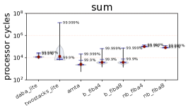
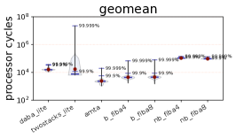
This section explores how the theoretical algorithmic complexity from the previous sections play out in practice. It explores how performance correlates with the number $n$ of entries in the window, the number $m$ of entries in the bulk insert or bulk evict, and the number $d$ of entries between an insertion and the youngest end of the window. The experiments use multiple monoidal aggregation operators to cover a spectrum of computational cost: sum (fast), geomean (medium), and bloom (Bloom, 1970) (slow).

This section refers to different sliding-window aggregation algorithms as follows: The original non-bulk FiBA algorithm (Tangwongsan et al., 2019) is nb_fiba4 and nb_fiba8, with MIN_ARITY of 4 or 8. Similarly, the new bulk FiBA algorithm introduced in this paper is b_fiba4 and b_fiba8. Both of these algorithms can handle out-of-order data. As baselines, several figures include three algorithms that only work for in-order data, i.e., when $d=0$. The amortized monoid tree aggregator, amta, supports bulk evict but not bulk insert (Villalba et al., 2019). The twostacks_lite algorithm performs single insert or evict operations in amortized $O(1)$ and worst-case $O(n)$ time (Tangwongsan et al., 2021). The daba_lite algorithm performs single insert or evict operations in worst-case $O(1)$ time (Tangwongsan et al., 2021). Since amta, twostacks_lite, and daba_lite require in-order data, they are absent from figures with results for out-of-order scenarios.

We ran all experiments on a machine with dual Intel Xeon Silver 4310 CPUs at 2.1 GHz running Ubuntu 20.04.5 with a 5.4.0 kernel. We compiled all experiments with g++ 9.4.0 with optimization level -O3. To reduce timing noise and variance in memory allocation latencies, we use mimalloc (Leijen et al., 2019) instead of the stock glibc allocator, and we pin all runs to core 0 and the corresponding NUMA group.

7.1. Latency

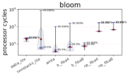
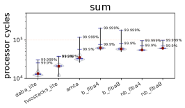
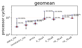
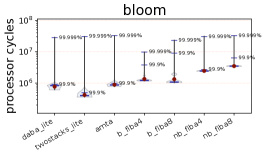
In streaming applications, late results are often all but useless: with increasing latency, the value of a streaming computation reduces sharply—for example, dangers become too late to avert and opportunities are missed. Therefore, our algorithm is designed to support both the finest granularity of streaming (i.e., when $m=1$) as well as bursty data (i.e., when $m\gg 1$) with low latencies. Even in the latter case, our algorithm still retains the ability of tuple-at-a-time streaming, unlike systems with a micro-batch model. The methodology for the latency experiments is to measure how long each individual insert or evict takes, then visualize the distribution of insertion or eviction times for an entire run as a violin plot. The plots indicate the arithmetic mean as a red dot, the median as a thick blue line, and the 99.9^th and 99.999^th percentiles as thin blue lines. At 2.1 GHz, $10^{4}$ processor cycles correspond to 4.8 microseconds.

Figure 7 shows the latencies for bulk evict with in-order data. This experiment loops over evicting the oldest $m=1,024$ entries in a single bulk, inserting 1,024 new entries one by one, and calling query, measuring only the time that the bulk evict takes. In theory, we expect bulk evict to take time $O(\log m)$ for b_fiba4 and b_fiba8, and $O(\log n)$ for amta. The remaining algorithms, lacking a native bulk evict, loop over single evictions, taking $O(m)$ time. In practice, b_fiba4, b_fiba8, and amta have the best latencies for this experiment, confirming the theory.

Figure 8 shows the latencies for bulk insert with in-order data. This experiment loops over evicting the oldest $m=1,024$ entries in a single bulk, inserting $m=1,024$ new entries in a single bulk, and calling query, measuring only the time that the bulk insert takes. In theory, since $d=0$ in this in-order scenario, the complexity of bulk insert boils down to $O(m)$ for all considered algorithms. In practice, daba-lite and twostacks-lite yield the best latencies for this scenario since they incur no extra overhead to be ready for an out-of-order case that does not occur here.

Figure 9. Latency, bulk insert only, window size $n=\textrm{4,194,304}$, bulk size $m=\textrm{1,024}$, out-of-order data $d=\textrm{1,024}$.

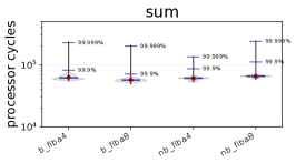
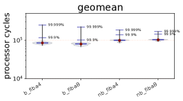
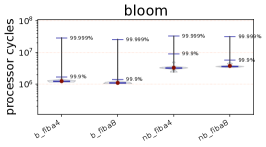
Figure 9 shows the latencies for bulk insert with out-of-order data. This experiment differs from the previous one in that each bulk insert happens at a distance of $d=1,024$ from the youngest end of the window. Since amta, twostacks_lite, and daba only work for in-order data, they cannot participate in this experiment. In theory, we expect bulk insert to take $O(m\log\frac{d}{m})$ for b_fiba and $O(m\log d)$ for nb_fiba, which is worse. In practice, b_fiba has lower latency than nb_fiba, confirming the theory.

Figure 10. Memory management ablation study (latency, bulk evict only, $n=\textrm{4,194,304}$, $m=\textrm{4,096}$, $d=0$).

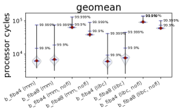
Figure 10 shows an ablation experiment for memory-management related implementation details. It compares results with mimalloc (mm) vs. the default memory allocator (libc), and with or without (nofl) the deferred free list from Section 6. Consistent with the theory, the deferred free list is indispensible: nofl performs much worse. On the other hand, mimalloc made little difference; we use it to control for events that are so rare that they did not manifest in this experiment.

7.2. Throughput

Throughput is the number of items in a long but finite stream divided by the time it takes to process that stream. The throughput experiments thus do not time each insert or evict operation individually. While the time for each individual operation may differ, we already saw those distributions in the latency experiments, and here we focus on the gross results instead. The experiments include a memory fence before every insert to prevent the compiler from optimizing (e.g., using SIMD) across multiple stream data items, as that would be unrealistic in fine-grained streaming. All throughput charts show error bars based on repeating each run five times.

Figure 11. Throughput, bulk evict only, window size $n=\textrm{4,194,304}$, varying bulk size $m$, in-order data $d=\textrm{0}$.

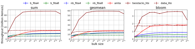
Figure 11 shows the throughput for running with bulk evict for in-order data as a function of the bulk size $m$. This experiment loops over a single call to bulkEvict for the oldest $m$ entries, $m$ calls to single insert, and a call to query. The throughput is computed from the time for the entire run, which includes all these operations. In theory, we expect the throughput of b_fiba and amta to improve with larger bulk sizes as they have native bulk eviction. In practice, while that is true, even for algorithms that do not natively support bulk evict, throughput also improves with larger $m$. This may be because their internal loop for emulating bulk evict benefits from compiler optimization. For in-order data, twostacks_lite yields the best throughput (but not the best latency, see Section 7.1).

Figure 12. Throughput, bulk evict+insert, window size $n=\textrm{4,194,304}$, varying bulk size $m$, in-order data $d=\textrm{0}$.

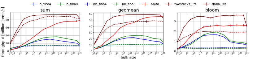
Figure 12 shows the throughput for running with both bulk evict and bulk insert for in-order data as a function of the bulk size $m$. In theory, we expect that since the data is in-order, bulk insert brings no additional advantage over looping over single inserts. In practice, all algorithms improve in throughput as $m$ increases from $2^{0}$ to around $2^{12}$. This may be because fewer top-level insertions means fewer memory fences, even for algorithms that emulate bulk insert with loops. Furthermore, throughput drops when $m$ gets very large, because the implementation needs to allocate more temporary space to hold data items before they are inserted in bulk.

Figure 13. Throughput, bulk evict+insert, window size $n=\textrm{4,194,304}$, bulk size $m=\textrm{1,024}$, varying ooo distance $d$.

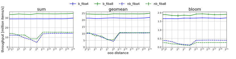
Figure 13 shows the throughput as a function of the out-of-order degree $d$ when running with both bulk evict and bulk insert. The amta, twostacks_lite, and daba algorithms do not work for out-of-order data and therefore cannot participate in this experiment. In theory, we expect that thanks to only doing the search once per bulk insert, higher $d$ should not slow things down. In practice, we find that that is true and b_fiba outperforms nb_fiba.

Figure 14. Throughput, bulk evict+insert, window size $n=\textrm{4,194,304}$, bulk size $m=\textrm{1}$, varying ooo distance $d$.

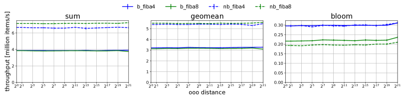
Figure 14 shows the throughput as a function of the out-of-order degree $d$ when running with neither bulk evict nor bulk insert, i.e. with $m=1$. As before, this experiment elides algorithms that require in-order data. In the absence of bulk operations, we expect b_fiba to have no advantage over nb_fiba. In practice, b_fiba does worse on sum and geomean but slightly better on bloom.

       

Figure 15. Histograms of (left) citi bike instantaneous window sizes $n$, (middle) eviction bulk sizes $m$ for a time-based window of 1 day, and (right) the out-of-order distance $d$, i.e., the number of records skipped over by insertions.

Figure 16. Throughput, citi bike, varying window size $n$, bulk size $m$ and ooo distance $d$ from real data.

7.3. Window Size One Billion

To understand how our algorithm behaves in more extreme scenarios, we ran b_fiba4 with geomean with a window size of 1 billion ($n=10^{9}$). In theory, FiBA is expected to grow to any window size and have good cache behaviors, like a B-tree. In practice, this is the case at window size 1B: The benchmark ran uneventfully using 99% CPU on average, fully utilizing the one core that it has. Memory occupancy per window item (i.e., the maximum resident set size for the process divided by the window size) stays the same ($64-70$ bytes), independent of window size.

However, at $n=1\mbox{B}$, the benchmark has a larger overall memory footprint, putting more burden on the memory system. This directly manifests as more frequent cache misses/page faults and indirectly affects the throughput/latency profile. While no major page faults occurred, the number of minor page faults per million tuples processed increased multiple folds (657 at $4\mbox{M}$ vs. 15,287 at $1\mbox{B}$). Compared with the 4M-window experiments, the throughput numbers for $n=1\mbox{B}$ mirror the same trends as the bulk size is varied. In absolute numbers, the throughput of $n=1\mbox{B}$ is $1-1.12\times$ less than that of $n=4\mbox{M}$. For latency, the theory promises $\log d$ average (amortized) bulk-evict time, independent of the window size. With a larger memory footprint, however, we expect a slight increase in median latency. The $\log n$ worst-case time should mean the rare spikes will be noticeably higher with larger window sizes. In practice, we observe that the median only goes up by $\approx 7.5\%$. The 99.999-th percentile markedly increases by around $2\times$.

7.4. Real Data

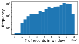
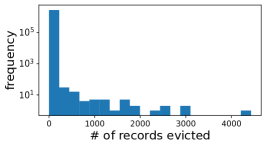
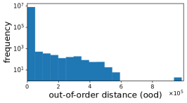
The previous experiments carefully controlled the variables $n$, $m$, and $d$ to explore tradeoffs and validate the theoretical results. It is also important to see how the algorithms perform on real data. Specifically, real applications tend to use time-based windows (causing both $n$ and $m$ to fluctuate), and real data tends to be out-of-order (with varying $d$). In other words, all three variables vary within a single run. Figure 15 shows this for the NYC Citi Bike dataset (cit, 2022) (Aug–Dec 2018). The figure shows a histogram of window sizes $n$ (left) and a histogram of bulk sizes $m$ (middle), assuming a time-based sliding window of 1 day. Depending on whether that 1 day currently contains more or fewer stream data items, $n$ ranges broadly, as one would expect for real data whose event frequencies are uneven. Similarly, depending on the timestamp of the newest inserted window entry, it can cause a varying number $m$ of the oldest entries to be evicted. Most single insertions cause only a single eviction, but there are a non-negligible number of bulk evicts of hundreds or thousands of entries. The figure also shows a histogram of out-of-order distances $d$ (right). While the vast majority of insertions have a small out-of-order distance $d$, there are also hundreds of insertions with $d$ in the tens of thousands.

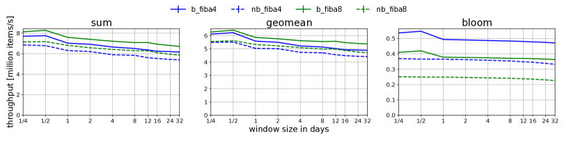
Figure 16 shows the throughput results for the Citi Bike dataset on a run that involves bulk evicts with varying $m$ and single inserts with varying $d$. Since amta, twostacks_lite, and daba require in-order data, we cannot use them here. In theory, we expect the bulk operations to give b_fiba an advantage over nb_fiba. In practice, we find that this is indeed the case for real-world data.

7.5. Java and Apache Flink

Figure 17. Throughput, Flink, bulk evict only, window size $n=\textrm{8,192}$, varying bulk size $m$, in-order data $d=\textrm{0}$.

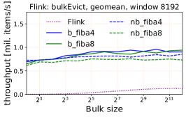
To experiment with our algorithm in the context of an end-to-end system, we reimplemented it in Java inside Apache Flink 1.17 (Carbone et al., 2015). We ran experiments that repeatedly perform several single inserts followed by a bulk evict and query. Using a window of size $n=2^{22}\approx 4\text{M}$, the FiBA algorithms perform as expected but the Flink baseline was prohibitively slow, so we report a comparison at $n=8,192$ instead. At this size, the trends are already clear. Figure 17 shows that even without our new bulk eviction support, FiBA is much faster than Flink. Using bulk evictions further widens that gap. As expected, throughput improves with increasing bulk size $m$, consistent with our findings with C++ benchmarks.

8. Conclusion

This paper describes algorithms for bulk insertions and evictions for incremental sliding-window aggregation. Such bulk operations are necessary for real-world data streams, which tend to be bursty. Furthermore, real-world data streams tend to have out-of-order data. Hence, besides handling bulk operations, our algorithms also handle that case. Our algorithms are carefully crafted to yield the same algorithmic complexity as the best prior work for the non-bulk case while substantially improving over that for the bulk case.(Tangwongsan et al., 2023)

Appendix A Proofs

Proof of Claim 1.

Let $k=\left\lfloor\frac{p}{\mu+1}\right\rfloor$. Then, $p=k(\mu+1)+r$, where $0\leq r\leq\mu$. There are two cases to consider: If $r=\mu$, set $t=k$ and $\beta_{t}=\mu$. Otherwise, $r\leq\mu-1$, set $t=k-1$ and $\beta_{t}=\mu+1+k\leq 2\mu$—i.e., the remainder is too small to be a valid node, so we combine them with the rightmost arity-$(\mu+1)$ node thus far. Notice that $t\geq 2$ since $p\geq 2\mu+2$. ∎

Further Discussion of Lemma 2. The amortized bound can be analyzed analogously to Lemma 9 in the FiBA paper (Tangwongsan et al., 2019), arguing that charging $2$ coins per new entry is sufficient in maintaining the tree. Below, we describe the extension from that proof that pertains to bulkInsert.

For a node $w$, we expect a coin reserve of

$$\small\textit{coins}(w)=\left\{\begin{array}[]{ll}2+2k&\mbox{if $a=2\mu+k$ and $k\geq 1$}\\ 2&\mbox{if $a=2\mu$ or ($a=\mu-1$ and $w$ is not the root)}\\ 1&\mbox{if $a=\mu$ and $w$ is not the root}\\ 0&\mbox{if $a<2\mu$ and ($a>\mu$ or $w$ is the root)}\end{array}\right.,$$

which naturally extends the coins function for arity $a\geq 2\mu+1$.

At the start of bulkInsert, we charge each entry $2$ coins, sufficient at the insertion sites. As restructuring happens, we reason about each affected node $w$ as follows: Let $t=\left\lfloor a/(\mu+1)\right\rfloor$, so $a=t(\mu+1)+r$, where $0\leq r\leq\mu$. There are two cases:

• $r=\mu$: Node $w$ yields $t-1$ new arity-$(\mu+1)$ nodes and one arity-$\mu$ node, needing $3(t-1)+4=3t+1$ coins to send up, pay for the split, and keep on the last node. But for $t\geq 2$, the reserve on $w$ has $\rho:=2(t(\mu+1)+\mu-2\mu+1)=2(t-1)\mu+2t+2\geq 2\frac{t}{2}\mu+2t+2\geq 4t+2$ as $\mu\geq 2$. Also, when $t=1$, $\rho=4\geq 3t+1$.

• $r\leq\mu-1$: Node $w$ yields $t-2$ new arity-$(\mu+1)$ nodes and one arity $(\mu+1+r)$ node, needing at most $3(t-2)+5=3t-1$ to send up, pay for the split, and keep on the last node (if $r=\mu-1$). Now we know $t\geq 2$. For $t\geq 3$, the reserve $\rho:=2(t(\mu+1)+r-2\mu+1)\geq 2(t-2)\mu+2t\geq 2\frac{t}{4}\mu+2t\geq 3t$ since $\mu\geq 2$. For $t=2$, $\rho=6+2r\geq 3t-1$.

Either way, the reserve coins can cover the restructuring cost.

Appendix B Pseudocode and Examples

Figures LABEL:fig:move_batch_example, LABEL:fig:merge_notsibling_example, and LABEL:fig:make_child_root_example provide pseudocode and more concrete examples for some of the core operations of our algorithm. To reduce clutter, the figures illustrate the tree structure with only timestamps. All three of these figures assume $\texttt{\small MIN\_ARITY}=2$, so each non-leaf node has between 2 and 4 children and each node has between 1 and 3 entries.

References

- (1)
- cit (2022) 2022. Citi Bike System Data. https://www.citibikenyc.com/system-data. Retrieved December, 2022.
- Agarwal et al. (2012) Pankaj K. Agarwal, Graham Cormode, Zengfeng Huang, Jeff Phillips, Zhewei Wei, and Ke Yi. 2012. Mergeable Summaries. In Symposium on Principles of Database Systems (PODS). 23–34. http://doi.acm.org/10.1145/2213556.2213562
- Akidau et al. (2013) Tyler Akidau, Alex Balikov, Kaya Bekiroglu, Slava Chernyak, Josh Haberman, Reuven Lax, Sam McVeety, Daniel Mills, Paul Nordstrom, and Sam Whittle. 2013. MillWheel: Fault-Tolerant Stream Processing at Internet Scale. In Conference on Very Large Data Bases (VLDB) Industrial Track. 734–746. https://doi.org/10.14778/2536222.2536229
- Bifet and Gavaldà (2007) Albert Bifet and Ricard Gavaldà. 2007. Learning from Time-Changing Data with Adaptive Windowing. In International Conference on Data Mining (ICDM). 443–448. https://doi.org/10.1137/1.9781611972771.42
- Bloom (1970) Burton H. Bloom. 1970. Space/Time Trade-offs in Hash Coding with Allowable Errors. Communications of the ACM (CACM) 13, 7 (1970), 422–426. https://doi.org/10.1145/362686.362692
- Bou et al. (2021) Savong Bou, Hiroyuki Kitagawa, and Toshiyuki Amagasa. 2021. CPiX: Real-Time Analytics Over Out-of-Order Data Streams By Incremental Sliding-Window Aggregation. Transactions on Knowledge and Data Engineering (TKDE) Early Access version of 28 January 2021 (2021). https://doi.org/10.1109/TKDE.2021.3054898
- Bouillet et al. (2012) Eric Bouillet, Ravi Kothari, Vibhore Kumar, Laurent Mignet, Senthil Nathan, Anand Ranganathan, Deepak S. Turaga, Octavian Udrea, and Olivier Verscheure. 2012. Processing 6 billion CDRs/day: from research to production (experience report). In Conference on Distributed Event-Based Systems (DEBS). 264–267. https://doi.org/10.1145/2335484.2335513
- Brown and Tarjan (1979) Mark R. Brown and Robert E. Tarjan. 1979. A Fast Merging Algorithm. Journal of the ACM (JACM) 26, 2 (April 1979), 211–226. https://doi.org/10.1145/322123.322127
- Carbone et al. (2015) Paris Carbone, Asterios Katsifodimos, Stephan Ewen, Volker Markl, Seif Haridi, and Kostas Tzoumas. 2015. Apache Flink: Stream and Batch Processing in a Single Engine. Bulletin of the IEEE Computer Society Technical Committee on Data Engineering 36, 4 (2015), 28–38. http://sites.computer.org/debull/A15dec/p28.pdf
- Cormen et al. (1990) Thomas Cormen, Charles Leiserson, and Ronald Rivest. 1990. Introduction to Algorithms. MIT Press.
- Hinze and Paterson (2006) Ralf Hinze and Ross Paterson. 2006. Finger trees: a simple general-purpose data structure. Journal of Functional Programming (JFP) 16, 2 (2006), 197–217. https://doi.org/10.1017/S0956796805005769
- Hirzel et al. (2017) Martin Hirzel, Scott Schneider, and Buğra Gedik. 2017. SPL: An Extensible Language for Distributed Stream Processing. Transactions on Programming Languages and Systems (TOPLAS) 39, 1 (March 2017), 5:1–5:39. https://doi.org/10.1145/3039207
- Izbicki (2013) Michael Izbicki. 2013. Algebraic Classifiers: A Generic Approach to Fast Cross-Validation, Online Training, and Parallel Training. In International Conference on Machine Learning (ICML). 648–656. http://proceedings.mlr.press/v28/izbicki13.html
- Kaplan and Tarjan (1995) Haim Kaplan and Robert E. Tarjan. 1995. Persistent Lists with Catenation via Recursive Slow-down. In Symposium on the Theory of Computing (STOC). 93–102. https://doi.org/10.1145/225058.225090
- Krishnamurthy et al. (2010) Sailesh Krishnamurthy, Michael J. Franklin, Jeffrey Davis, Daniel Farina, Pasha Golovko, Alan Li, and Neil Thombre. 2010. Continuous Analytics over Discontinuous Streams. In International Conference on Management of Data (SIGMOD). 1081–1092. https://doi.org/10.1145/1807167.1807290
- Leijen et al. (2019) Daan Leijen, Benjamin Zorn, and Leonardo de Moura. 2019. Mimalloc: Free List Sharding in Action. In Asian Symposium on Programming Languages and Systems (APLAS). 244–265. https://doi.org/10.1007/978-3-030-34175-6_13
- Li et al. (2008) Jin Li, Kristin Tufte, Vladislav Shkapenyuk, Vassilis Papadimos, Theodore Johnson, and David Maier. 2008. Out-of-Order Processing: A New Architecture for High-performance Stream Systems. In Conference on Very Large Data Bases (VLDB). 274–288. https://doi.org/10.14778/1453856.1453890
- Michalke et al. (2021) Adrian Michalke, Philipp M. Grulich, Clemens Lutz, Steffen Zeuch, and Volker Markl. 2021. An Energy-Efficient Stream Join for the Internet of Things. In Workshop on Data Management on New Hardware (DaMoN). https://doi.org/10.1145/3465998.3466005
- Poppe et al. (2021) Olga Poppe, Chuan Lei, Lei Ma, Allison Rozet, and Elke A. Rundensteiner. 2021. To Share, or Not to Share Online Event Trend Aggregation Over Bursty Event Streams. In International Conference on Management of Data (SIGMOD). 1452–1464. https://doi.org/10.1145/3448016.3452785
- Seidemann et al. (2019) Marc Seidemann, Nikolaus Glombiewski, Michael Körber, and Bernhard Seeger. 2019. ChronicleDB: A High-Performance Event Store. Transactions on Database Systems (TODS) 44, 4 (Oct. 2019). https://doi.org/10.1145/3342357
- Shein et al. (2017) Anatoli U. Shein, Panos K. Chrysanthis, and Alexandros Labrinidis. 2017. FlatFIT: Accelerated Incremental Sliding-Window Aggregation for Real-Time Analytics. In Conference on Scientific and Statistical Database Management (SSDBM). 5.1–5.12. https://doi.org/10.1145/3085504.3085509
- Tangwongsan et al. (2019) Kanat Tangwongsan, Martin Hirzel, and Scott Schneider. 2019. Optimal and General Out-of-Order Sliding-Window Aggregation. In Conference on Very Large Data Bases (VLDB). 1167–1180. http://www.vldb.org/pvldb/vol12/p1167-tangwongsan.pdf
- Tangwongsan et al. (2021) Kanat Tangwongsan, Martin Hirzel, and Scott Schneider. 2021. In-Order Sliding-Window Aggregation in Worst-Case Constant Time. Journal on Very Large Data Bases (VLDB J.) 30 (June 2021), 933–957.
- Tangwongsan et al. (2023) Kanat Tangwongsan, Martin Hirzel, and Scott Schneider. 2023. Out-of-Order Sliding-Window Aggregation with Efficient Bulk Evictions and Insertions (Extended Version). [this document].
- Theodorakis et al. (2018) Georgios Theodorakis, Alexandros Koliousis, Peter R. Pietzuch, and Holger Pirk. 2018. Hammer Slide: Work- and CPU-efficient Streaming Window Aggregation. In Workshop on Accelerating Analytics and Data Management Systems Using Modern Processor and Storage Architectures (ADMS). 34–41. http://adms-conf.org/2018-camera-ready/SIMDWindowPaper_ADMS’18.pdf
- Theodorakis et al. (2020a) Georgios Theodorakis, Alexandros Koliousis, Peter R. Pietzuch, and Holger Pirk. 2020a. LightSaber: Efficient Window Aggregation on Multi-core Processors. In International Conference on Management of Data (SIGMOD). 2,505–2,521. https://dl.acm.org/doi/10.1145/3318464.3389753
- Theodorakis et al. (2020b) Georgios Theodorakis, Peter R. Pietzuch, and Holger Pirk. 2020b. SlideSide: A fast Incremental Stream Processing Algorithm for Multiple Queries. In Conference on Extending Database Technology (EDBT). 435–438. https://openproceedings.org/2020/conf/edbt/paper_337.pdf
- Traub et al. (2019) Jonas Traub, Philipp Grulich, Alejandro Rodriguez Cuellar, Sebastian Bres̈, Asterios Katsifodimos, Tilmann Rabl, and Volker Markl. 2019. Efficient Window Aggregation with General Stream Slicing. In Conference on Extending Database Technology (EDBT). 97–108. https://doi.org/10.5441/002/edbt.2019.10
- Villalba et al. (2019) Alvaro Villalba, Josep Lluis Berral, and David Carrera. 2019. Constant-Time Sliding Window Framework with Reduced Memory Footprint and Efficient Bulk Evictions. Transactions on Parallel and Distributed Systems (TPDS) 30, 3 (May 2019), 486–500. https://doi.org/10.1109/TPDS.2018.2868960