Mass–accretion, spectral, and photometric properties of T Tauri stars in Taurus based on TESS and LAMOST

Abstract

We present the analysis of 16 classical T Taur stars using LAMOST and TESS data, investigating spectral properties, photometric variations, and mass-accretion rates. All 16 stars exhibit emissions in H$\alpha$ lines, from which the average mass-accretion rate of $1.76\times 10^{-9}~{}M_{\odot}yr^{-1}$ is derived. Two of the stars, DL Tau and Haro 6–13, show mass–accretion bursts simultaneously in TESS, ASAS–SN, and/or ZTF survey. Based on these observations, we find that the mass–accretion rates of DL Tau and Haro 6–13 reach their maximums of $2.5\times 10^{-8}~{}M_{\odot}yr^{-1}$ and $2\times 10^{-10}~{}M_{\odot}yr^{-1}$ during the TESS observation, respectively. We detect thirteen flares among these stars. The flare frequency distribution shows that the CTTSs’ flare activity is not only dominated by strong flares with high energy but much more active than those of solar-type and young low–mass stars. By comparing the variability classes reported in the literature, we find that the transition timescale between different classes of variability in CTTSs, such as from Stochastic (S) to Bursting (B) or from quasi-periodic symmetric (QPS) to quasi-periodic dipping (QPD), may range from 1.6 to 4 years. We observe no significant correlation between inclination and mass–accretion rates derived from the emission indicators. This suggests that inner disk properties may be more important than that of outer disk. Finally, we find a relatively significant positive correlation between the asymmetric metric M and the cold disk inclination compared to the literature. A weak negative correlation between the periodicity metric Q value and inclination has been also found.

1 Introduction

Classical T Tauri stars (CTTSs) are young, low-mass pre–main–sequence objects with typical spectral types between F and M, that are accreting material from the circumstellar disk. These stars exhibit strong emission lines in their spectra and show an excess of emission ranging from radio to ultraviolet relative to the stellar photosphere. The infrared excess emission from CTTS indicates the presence of a circumstellar disk (Mendoza V., 1968; Lynden-Bell & Pringle, 1974; Adams et al., 1987; Bertout et al., 1988) and can be used to infer the amount of dust and the evolutionary status of the system. The amount of circumstellar material drops as the protostellar system evolves, leading to the decrease of the excess emission in the infrared.

The CTTSs have luminosity variations on different timescales, from hours to even decades (Rucinski et al., 2008; Cody et al., 2013), depending on various physical phenomena affecting the stellar and circumstellar environment. For example, the obscuration of the central star’s photosphere by circumstellar dust may lead to an aperiodic dip of light (e.g., McGinnis et al., 2015). The presence of stable starspots on the stellar surface may result in a periodic modulation in the light curve of the star (e.g., Kóspál et al., 2018). The unsteady accretion processes and magnetic activity (i.e., flares) may cause the random and short timescale brightening variability. The stochastic light curve of the CTTS may be attributed to the superposition of the various types of variability resulting from different mechanisms mentioned earlier. All these mechanisms can vary with time.

One of the major sources of variability in CTTSs during this evolutionary phase is the accretion–driven burst (e.g., Fischer et al., 2022). There are various types of accretion–driven bursts that last for different timescales. One type is the FU Ori–like outburst, which is characterized by a large increase in luminosity (typically by a factor of tens) over a timescale of decades to hundreds of years (e.g., Clarke et al., 2005). In addition, the outbursts with the type of V1647 Ori, EX Lup, and Protostellar share the similar timescale of a few years with a luminosity increase ranging from 1 to 5 mag. Lastly, the one we focus on in this study is the accretion bursts with a luminosity variability up to a few magnitudes on a relatively short timescales from a few hours to days at optical wavelengths (e.g., Cody & Hillenbrand, 2018). The numerical simulations carried out by (e.g., Čemeljić & Siwak, 2020) suggest that this variability could be caused by unstable accretion processes. In addition, such events, coupled with rotational modulation, tend to dominate changes in the accretion rate (Rigon et al., 2017; Sergison et al., 2020).

According to the magnetospheric accretion mechanism (e.g., Camenzind, 1990), the most viable scenario currently used to describe the accretion behaviors of CTTSs, the central star is channeling the material in the circumstellar disk to the stellar surface through the magnetospheric accretion columns (Feigelson & Montmerle, 1999; Muzerolle et al., 2003). The gas is heated to a temperature of $10^{4}$–$10^{6}$ K when the channeled materials hit the stellar surface, creating a shock on the stellar photosphere, which emits intense X–rays (Argiroffi et al., 2007; Günther et al., 2007; Costa et al., 2017). The X–rays are mostly reabsorbed by the accretion columns, from which the lower energy photons, mainly in blue band, are re–emitted, resulting in the luminosity excess from visible to ultraviolet wavelength. Thus, the U–band excess has been often used to determine the accretion luminosity, from which the mass–accretion rate can be determined (Gullbring et al., 1998; Herczeg & Hillenbrand, 2008). In addition, such an accretion mechanism also produces detectable emission features in CTTSs spectra, such as H$\alpha$ and H$\beta$ (e.g., Basri & Bertout, 1989). Sousa et al. (2016) shows that when U–band excesses are not available, mass-accretion rates can be obtained with good results from the H$\alpha$ flux using the currently available calibrations from the literature. Therefore, these emission features can be used to probe the state (i.e., active or inactive) of the mass–accretion process. Furthermore, multi–band simultaneous observations can be useful for estimating the mass-accretion rate of CTTSs even without direct U–band measurements. For example, Tofflemire et al. (2017) and Kóspál et al. (2018) used optical wavelength observations of accretion burst variability to estimate the mass-accretion rate of DQ Tau. In Kóspál et al. (2018), they used the Kepler light curve to identify the burst phenomenons and extrapolated the associated U–band excess luminosities based on the simultaneous BVRI observations of the star.

In this study, we present mass–accretion rates and the properties that can be determined with our data for selected CTTSs in the Taurus Molecular Cloud (hereafter, TMC), which is a nearby star–forming region located at a distance about 147 pc from the Sun (Zucker et al., 2020) with an age of 1–3 Myr (Simon et al., 2017), using high photometric precision light curves and low–resolution spectra from the space–based telescope, TESS (the Transiting Exoplanet Survey Satellite) and LAMOST (the Large Sky Area Multi–Object Fibre Spectroscopic Telescope), respectively. Given the lengths of the available light curve data, we will primarily focus on the short timescale burst.

The outline of this paper is as follows. In Section 2, we introduce the TESS and LAMOST observations of TMC members, including their stellar parameters reported in literature. In Section 3, we explain our methodology for estimating the mass–accretion rates of our CTTS targets using various emission indicators from LAMOST low-resolution spectra and TESS light curves. We also detail our method for determining photometric variabilities in this section. In Section 4, we describe our results of the data analysis and implications. Finally, in Section 5, we summarize the result and conclude the study.

2 Sample and data sets

2.1 LAMOST spectroscopic survey on T Tauri stars

LAMOST, the Large Sky Area Multi–Object Fibre Spectroscopic Telescope located at the Xinglong Observatory of the National Astronomical Observatories of Chinese Academy of Sciences (NAOC), is a reflecting Schmidt telescope with an effective aperture of $\sim 4$ m and a wide field of view of 20 deg² in the sky (Zhao et al., 2012).

With 4000 fibers that are mounted on the focal plane, it has been conducting spectroscopic surveys efficiently for stars, galaxies and quasars mostly in the northern celestial hemisphere above the declination of $-10$ degree since Autumn 2012. Each fiber has a scale of 3.3 arcseconds on the focal surface. The centers of the spectroscopic fibers are about 4.47 arcminutes apart, and each fiber can move at most 3 arcminutes from its center position. Sixteen spectrographs are used in the system, and each receives the dispersed light from 250 fibers. The resolution of LAMOST spectra is R $\approx$ 1800 around the sdss–g band with a wavelength coverage of 3700–9100 Å.

The LAMOST 2D pipeline is utilized for data reduction. Initially, each exposure’s data from each CCD chip is separately reduced, and then the results from each exposure are combined. Bias and dark are subtracted from each raw image. The flat-field spectrum of each fiber is traced, and a polynomial is fitted to the centroid of each fiber’s row position. A Gaussian-like profile is assumed for each fiber’s profile in the row direction. Using the same trace function, spectra are extracted from all data on the same night, with minor shifts made to align individual frames. The extracted spectra are divided by the one-dimensional flat-field spectrum. The Hg/Cd and Ne/Ar arc lamp spectra are also extracted using the same trace function, including strong sky emission lines to further improve the wavelength solution. The sky spectra are obtained from 20 sky fibers allocated in each spectrograph. After wavelength calibration, all sky spectra are combined into one super-sky spectrum. The super-sky spectrum is scaled to best fit the sky spectrum in each fiber, and then this scaled super-sky is subtracted from each fiber, and the telluric absorption is removed. The science spectra are flux-calibrated by matching the selected flux standard stars and their templates, which are usually of spectral type A or F. Up to five flux standard stars are observed per spectrograph.

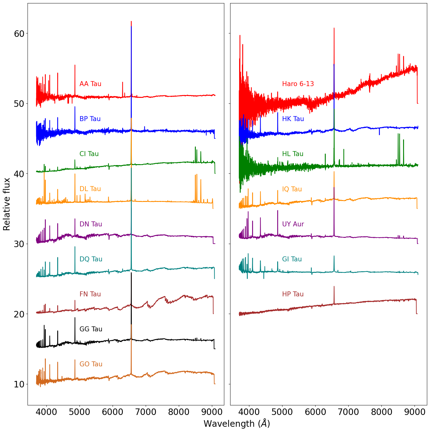
Figure 1: The LAMOST low–resolution spectra of 16 CTTSs in this study

We retrieved spectroscopic data of CTTSs in the TMC from LAMOST’s decade–long archive of observational data, and 16 targets are identified (see Table 1). The LAMOST low–resolution spectra of these CTTSs are shown in Figure 1. Table 2 contains the stellar parameters of our targets. The masses and radii of most CTTSs are provided in Herczeg & Hillenbrand (2014), with the exception of HL Tau. The radius (R=7 R_⊙) and mass (M=1.7M_⊙) of HL Tau are given by Liu et al. (2017) and Pinte et al. (2016), respectively. The inclinations of the outer disk have been reported by the adaptive optics (i.e., Close et al., 1998), millimeter radio (i.e., Guilloteau et al., 1999), high–resolution near–infrared imaging (Kudo et al., 2008), and high–resolution submillimeter resolved image observations of the TMC region (ALMA Partnership et al., 2015; Long et al., 2019; Manara et al., 2019; Villenave et al., 2020). The distance information for the objects studied in this work is from the parallax measurements reported in Gaia Collaboration (2020). HK Tau is a binary system consisting of two companions, HK Tau A and HK Tau B, with HK Tau A being much brighter than HK TauB ($G$=14.106 vs $G$=17.962 (Gaia Collaboration et al., 2021)). The disk inclinations of the two companions are highly misaligned, with HK Tau A having an inclination of $i$=56.9^o (Manara et al., 2019) and HK Tau B having an inclination of $i$=84^o (Villenave et al., 2020). Therefore, we list their inclinations together in the Table and treat them as an uncertainty in our result comparison in the later sections.

2.2 TESS observations of T Tauri stars in TMC

TESS (the Transiting Exoplanet Survey Satellite) is an MIT–led NASA mission launched on April 18, 2018, to search for nearby transiting exoplanets using the fast–sampling (2–minute) time–series data with the high photometric precision, which is also well suited for studies of stellar physics. The Taurus Molecular Cloud was in the field of view of TESS in Sectors 43 and 44 from 2021 September 16 to 2021 November 6. Fourteen of our LAMOST CTTS targets have released TESS 2–min cadence light curve data (see Table 1).

There are two kinds of flux information contained in the TESS data: Simple Aperture Photometric flux (SAP) and the Pre-search Data Conditioning Simple Aperture Photometric flux (PDCSAP). The SAP flux is produced by summing the count rates of the pixels within a customized aperture given by the Science Processing Operations Center (SPOC) pipeline (Jenkins et al., 2016). The SAP flux is often affected by systematic errors such as long term trend, which have been removed from the PDCSAP flux using Co–trending Basis Vectors. Therefore, the PDCSAP flux is often cleaner than SAP flux. In this study, we use the PDCSAP flux data with good quality (flag bits QUALITY$=$0) in our analyses. Although the long term trends might be the true signal of the stars, the unsteady accretion flows have relatively short timescales and should not be affected significantly by removing the long term trend signal.

Considering the large size of the TESS pixel scale ($21^{{}^{\prime\prime}}\times 21^{{}^{\prime\prime}}$), the contamination due to the nearby sources in crowded regions may be unavoidable. To investigate whether the light curves of our targets of interest are contaminated by the neighboring stars, the Python package Lightkurve (Lightkurve Collaboration et al., 2018) were employed. We downloaded the target pixel file (TPF) of each star and plotted it together with the coordinates of the field stars with G_RP mag $<$ 15 queried from Gaia DR3 (Gaia Collaboration, 2020). The left panel in Figure 2 is an example, the TPF of GG Tau (TIC 245830955). The pink mask region is the SPOC pipeline aperture, the red hollow circles are the locations of the field stars, and GG Tau is marked by a red filled circle. In addition to GG Tau, there is one neighboring star within the SPOC aperture. The neighbor star (G${}_{RP}\sim 13$) is much fainter than GG Tau (G${}_{RP}\sim 10$). Also, the overall shapes of the light curves extracted using various test apertures do not change significantly compared to the light curve from SPOC aperture. As the result, the SPOC given PDCSAP flux of GG Tau is reliable for the following research. The right panel in Figure 2 shows another example, GI Tau (TIC 268444803). There are three neighbor stars within or at the edge of the SPOC aperture of GI Tau. One of them is GK Tau (G${}_{RP}=$ 10.89) and is about equally bright to GI Tau (G${}_{RP}=$ 11.5). After the examination with different test apertures, we found that it is impossible to distinguish the variability feature between GI Tau and the field stars in the light curve. Therefore, the GI Tau data was excluded from following analysis. In the same way, HL Tau has a similar problem with GI Tau and was also excluded. Ultimately, there were only 12 targets for which the data could be used in the subsequent analyses.

3 Analysis

3.1 Calibrating relative flux of LAMOST data to absolute unit

Due to the limited number of spectral standard stars in the LAMOST survey, no absolute flux-corrected data are available, only relative flux-corrected data can be used. To obtain the physical flux information, we adopt the template spectra of weak–lines T Tauri stars (WTTS) with the spectral type ranging from K5 to M7 provided by Manara et al. (2013). We first normalize the template spectra and LAMOST spectra using the mean flux between 7750 and 8000 $\AA$ because this range has relatively few emission/absorption features. In this way, we find the best–fit template spectra with the corresponding spectral types for every LAMOST spectra. We then convert the normalized flux of the template spectra and LAMOST spectra back to the physical flux level of template spectra before normalization. Finally, the absolute calibrated flux density of LAMOST data (F_λ,cal) is obtained by using the following equation:

$$F_{\lambda,cal}=F_{\lambda,tem}(\frac{d_{2}}{d_{1}})^{2},$$ (1)

where F_λ,tem is the flux density of the best–fit template spectra, the d₂ is the distance in parsecs of the template star given by Manara et al. (2013), and d₁ is the distance in parsecs of our sample.

To ensure the accuracy of our calibrated absolute flux measurements, we have cross-checked our results with photometric data obtained by ASAS–SN (Jayasinghe et al., 2018, 2019) and Pan–STARRS (Chambers et al., 2016; Flewelling et al., 2020) surveys if any, which were taken within 20 days of the LAMOST observation date. As CTTSs are known to be highly variable stars, this additional step provides further validation of our flux calibration. In these surveys, we have identified the following stars in our samples with the photometric data that meet the criteria: (1) from ASAS–SN: AA Tau in the sdss–g band and BP Tau in the V band, (2) from Pan–STARRS sdss–g band: DL Tau, DN Tau, Haro 6–13, HL Tau, and IQ Tau, and (3) from Pan–STARRS sdss–i band: GO Tau and HK Tau. The flux (in mJy) and observation date (in MJD) of the these photometric data are listed in Table 3. We convert the flux units of the survey photometric data from mJy to the same units as our calibrated LAMOST spectra. Next, we scale the calibrated LAMOST spectra to match the flux from the surveys at the effective wavelength of the corresponding band. This allows us to obtain a more accurate calibrated flux for our LAMOST data. Figure 3 shows the example spectra of the flux calibration processes of three stars: DL Tau, AA Tau, and GO Tau. For stars that lack survey photometric data, we still use their spectra in the following analysis. However, we note that the results obtained from these data could be uncertain by an order of 0 to 1.

3.2 Mass–accretion rate measurements from LAMOST spectra analysis

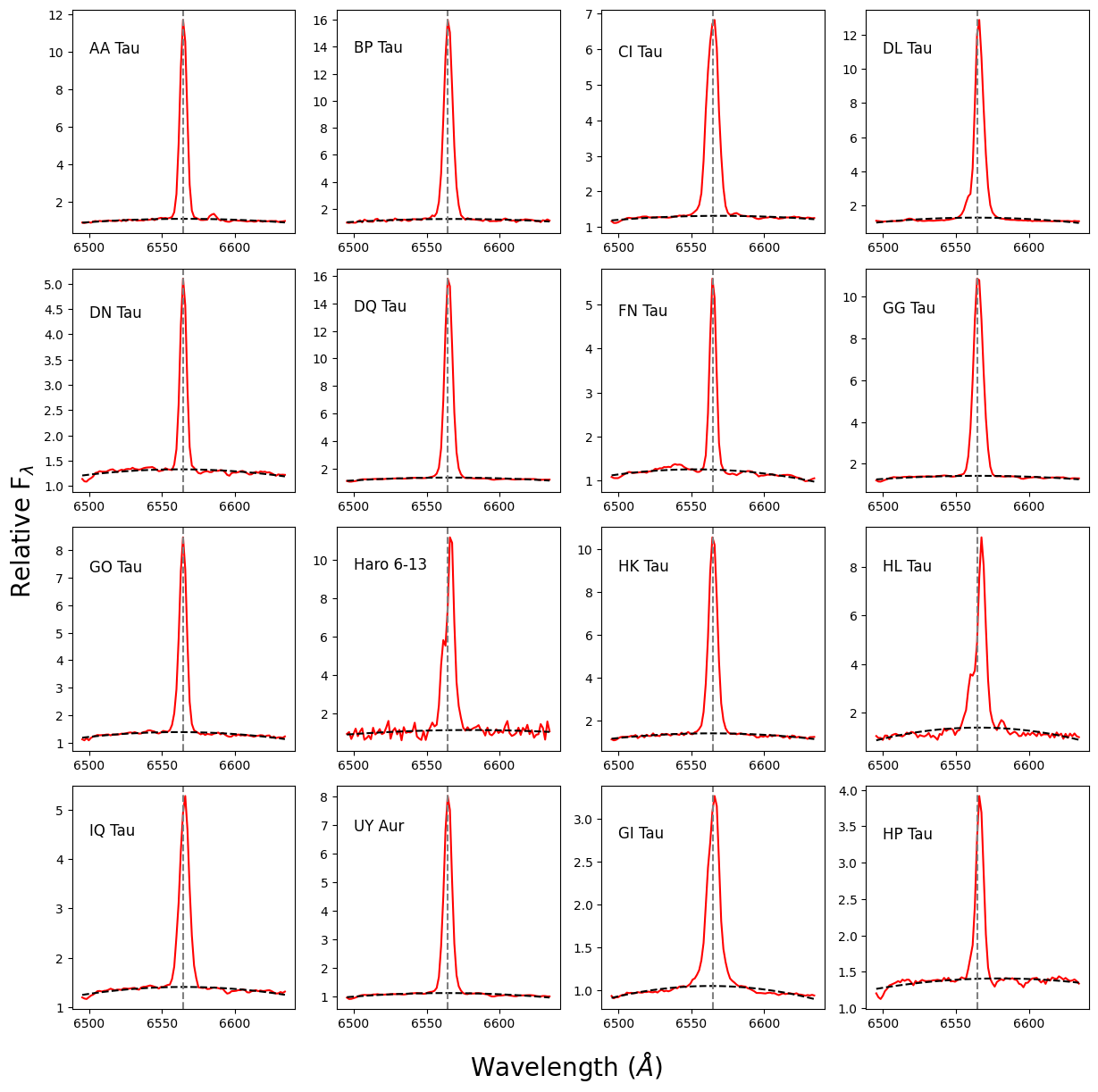
Figure 4: H$\alpha$ emission profiles of our targets observed by LAMOST. In each panel, the spectra is displayed in red, and the black line represents the fit local continuum. The dash vertical line in gray marks the center wavelength of the H$\alpha$ line.

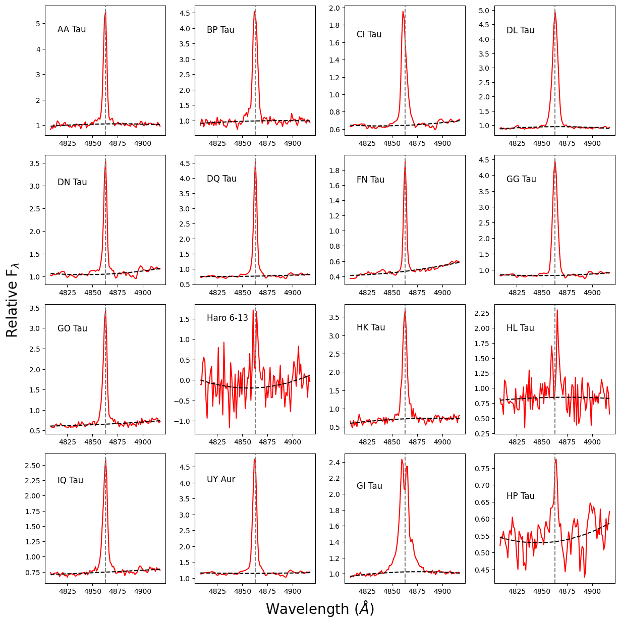
Figure 5: H$\beta$ emission profiles of our targets observed by LAMOST. Dashed vertical gray line represents the center of the line in each panel.

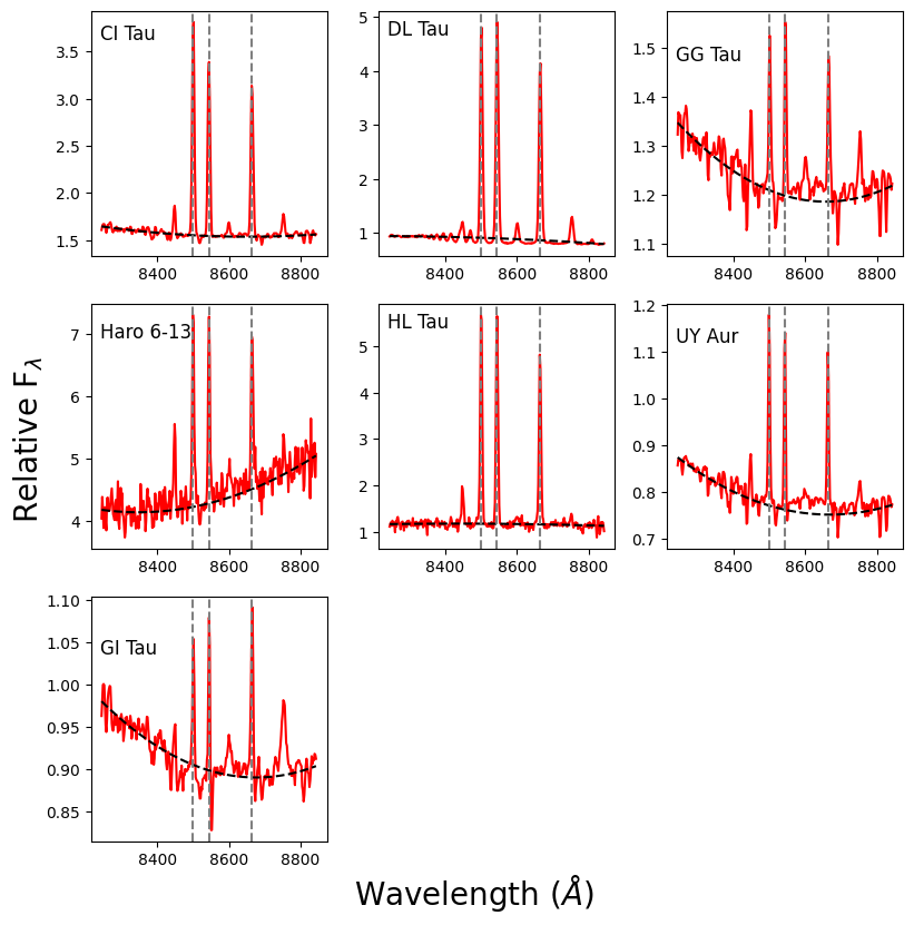
Figure 6: Ca$\text{II}$ 8498, 8542, 8662 $\AA$ emission profiles of our targets observed by LAMOST. Dashed vertical gray lines represent the center of the Ca$\text{II}$ triplet lines in each panel.

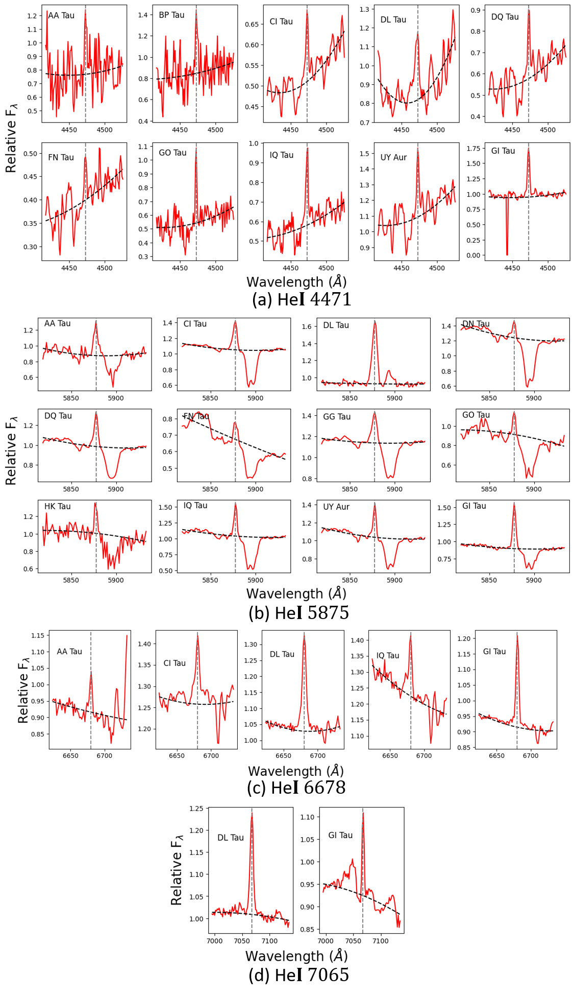
Figure 7: He$\text{I}$ 4471 (a), 5875 (b), 6678 (c), 7065 (d) emission profiles of our targets observed by LAMOST. Dashed vertical gray line represent the center of the He$\text{I}$ in each panel.

Using the LAMOST low–resolution spectral data, we are able to estimate the mass–accretion rates of T Tauri stars by analyzing various permitted emission lines of H$\alpha$ 6563 $\AA$, H$\beta$ 4861 $\AA$, Ca$\text{II}$ 8498, 8542, 8662 $\AA$, and He$\text{I}$ 4471, 5875, 6678, 7065 $\AA$ (Fang et al., 2009; Herczeg et al., 2009; Alcalá et al., 2014, 2017), which are generated by the accretion flows between the disc and star, in the available wavelength coverage. The emission profiles of these lines in all spectra are shown in Figure 4, Figure 5, Figure 6, and Figure 7.

For each spectrum, we first estimate the equivalent width (EW) of the emissions with the equation:

$$EW=\int(\frac{F_{\lambda}}{F_{o}}-1)d\lambda,$$ (2)

where $F_{\lambda}$ is the spectral flux of the line defined to be within the 3–$\sigma$ of the best–fit Gaussian model with the central wavelength of the particular line; $F_{o}$ is the average flux of the continuum in the same range. The equivalent widths of all available emissions in the spectra are listed in Table 5. Then, the emission’s flux ($F_{em}$) as well as their luminosities ($L_{em}$) can be obtained using the following equations:

$$F_{em}=EW_{em}F_{c}(em),$$ (3)

$$L_{em}=4\pi d^{2}F_{em}.$$ (4)

Here, the $EW_{em}$ represents the equivalent width of the emission, $F_{c}(em)$ is the local continuum flux in the emission’s wavelength range, and $d$ is the distance to the stars. The mass–accretion luminosity ($L_{acc}$) of T Tauri star can be determined from the line luminosity ($L_{line}$) by using the relation below:

$$log(L_{acc}/L_{\odot})=b+a*log(L_{line}/L_{\odot}),$$ (5)

where $L_{\odot}$ is the solar luminosity. The coefficients $a$ and $b$ of every line used in the study is given by Alcalá et al. (2017) (see Tabel B.1. in their paper). If the accretion energy is reprocessed fully into the accretion continuum, the $L_{acc}$ can be converted into the mass–accretion rate ($\dot{M}_{acc}$) using the following equation from Herczeg & Hillenbrand (2008):

$$\dot{M}_{acc}=\frac{L_{acc}R_{*}}{GM_{*}(1-\frac{R_{*}}{R_{in}})},$$ (6)

where $M_{*}$ is the stellar mass, $G$ is the gravitational constant, $R_{*}$ is the stellar radius, and $R_{in}$ is the inner radius of the disk, which is defined as the disk truncation radius of CTTSs with a standard value of $5R_{*}$ (Gullbring et al., 1998). The estimated mass–accretion rates from all available emissions are displayed in Table 6.

3.3 Variability of our CTTSs sample

A statistical metric system reported by Cody et al. (2014) allows the light curves of young stellar objects to be classified into different categories, thus it is useful to recognize the burst–like accretion events in the TESS light curves of our samples. The system contains two metrics: the flux asymmetry (denoted as M), and the quasi–periodicity (denoted as Q). The metric M is the first one we focus here, which represents the light curve behavior tendency of dipping (M $>0$) and bursting (M $<0$). We determine the metric M following the approach explained in detail by Cody & Hillenbrand (2018) (see Sec. 5. in their paper). We first normalize the light curve with the median of the flux and smooth it with 200 points moving mean. After subtracting the smoothed light curve from the original one, we identify the 5$\sigma$ outliers in the residual curve and remove their counterparts from the original curve. Then the metric M is estimated using the formula:

$$M=-(f_{5\%}-f_{med})/\sigma_{f},$$ (7)

where $f_{5\%}$ is the mean of the first and last 5 percent of the fluxes in the outlier–free curve, and $f_{med}$ and $\sigma_{f}$ are the median flux and the rms of the original curve, respectively. Stars with M $<-0.25$ are likely to display the accretion–like burst variability in their light curves. The M–values of all of these CTTSs are listed in Table 4.

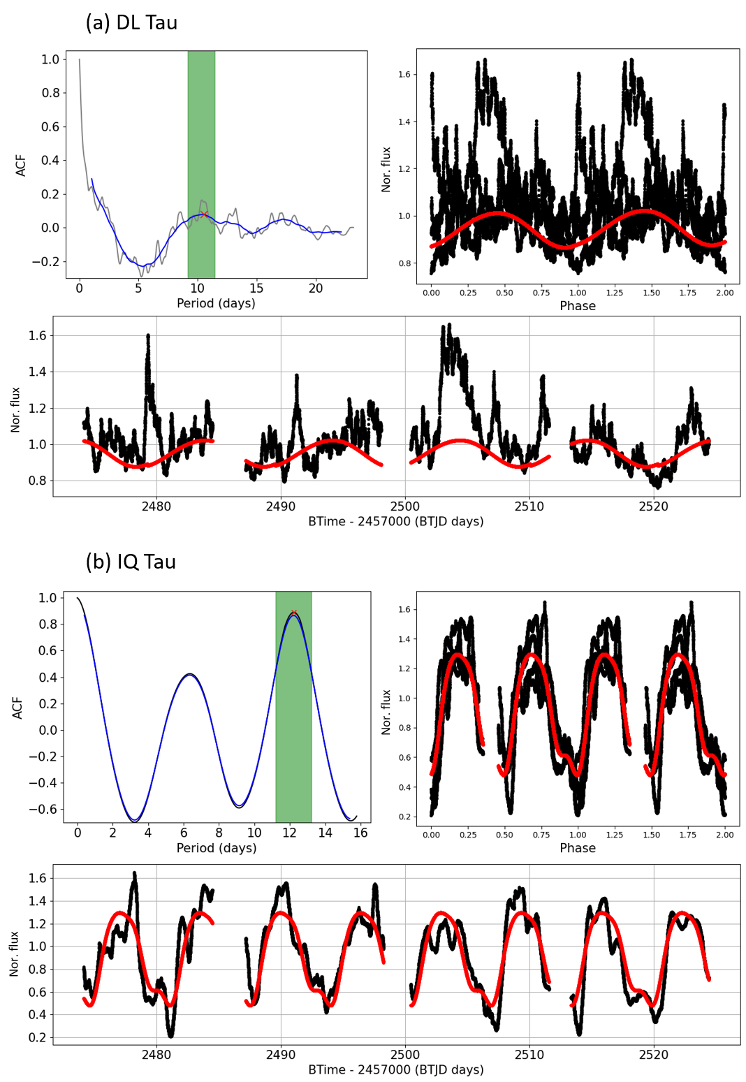
Figure 8: The examples of the period re-/estimate of the CTTSs, here shows (a) DL Tau and (b) IQ Tau. In each case, the upper left panel shows the autocorrelation function. The gray one is the original ACF, the blue one is a smoothed version of the ACF. The red cross marks the peak of the ACF, and the FHWM highlighted by green, from where the best period is determined. The upper right panel is the phase curve (black) and the best Gaussian Process fit curve (red). The panel at the bottom is the full TESS Section 43 and 44 light curve of the star (black) with the best Gaussian Process fit curve (red). The best periods we found for DL Tau and IQ Tau are 10.4 day and 12.9 day, respectively.

The second metric Q is used to evaluate periodicity tendency of light curves in the range from Q=0 (purely periodic) to Q=1 (stochastic) (Cody et al., 2014). To determine the Q–values of the light curve, we first fold up the light curves with the associated periods reported by Percy et al. (2010) and Rebull et al. (2020) if any. One special case is DQ Tau, which is a spectrocopic binary and has two reported brightness variation periods: $\sim 15.8$ day and $\sim 3.03$ day. The first one is attributed to the brightening effect associated with mass–accretion and magnetic reconnection that occurs around the periastron when two stars approach each other (Mathieu et al., 1997; Salter et al., 2010; Czekala et al., 2016; Getman et al., 2016). The second one is the rotational modulation caused by the presence of the spots, and we use it to determine the $Q$-value for DQ Tau. Since the morphologies of variability in young stellar objects could vary with time (e.g., Sousa et al., 2016), we manually examine the phase curve to ensure the validity of the reported periods for our data. If the star has no reported period, or if the reported period is not applicable to our data, we re–/determine the period by, firstly, identifying the maximum in the autocorrelation function and, secondly, refining the period within the full height width of the maximum (FHWM). The best period solution is determined by selecting the one that provides the optimal folded phase curve counterpart. This selection process involves manually examining the phase curves and comparing them to those from other potential period values. Figure 8 illustrates DL Tau and IQ Tau as examples, with estimated periods of 10.4 day and 12.9 day, respectively. Next, we use the Gaussian Process (GP) to produce a smooth light curve pattern with the optimal period, which is then subtracted from the original light curve to measure the residual noise. Finally, the resulting residual variance is divided by the variance of the original light curve to obtain the Q-value.

We then divide the light curves of our samples into eight different categories using the definition of Q and M ranges given by Cody et al. (2022):

1. Burster (B): $M<-0.25$

2. Purely periodic symmetric (P): $Q<0.15$ and $-0.25<M<0.25$

3. Quasiperiodic symmetric (QPS): $0.15<Q<0.85$ and $-0.25<M<0.25$

4. Purely stochastic (S): $Q>0.85$ and $-0.25<M<0.25$

5. Quasiperiodic dipper (QPD): $0.15<Q<0.85$ and $M>0.25$

6. Aperiodic dipper (APD): $Q>0.85$ and $M>0.25$

7. Long timescale (L)

8. Variable but unclassifiable (U)

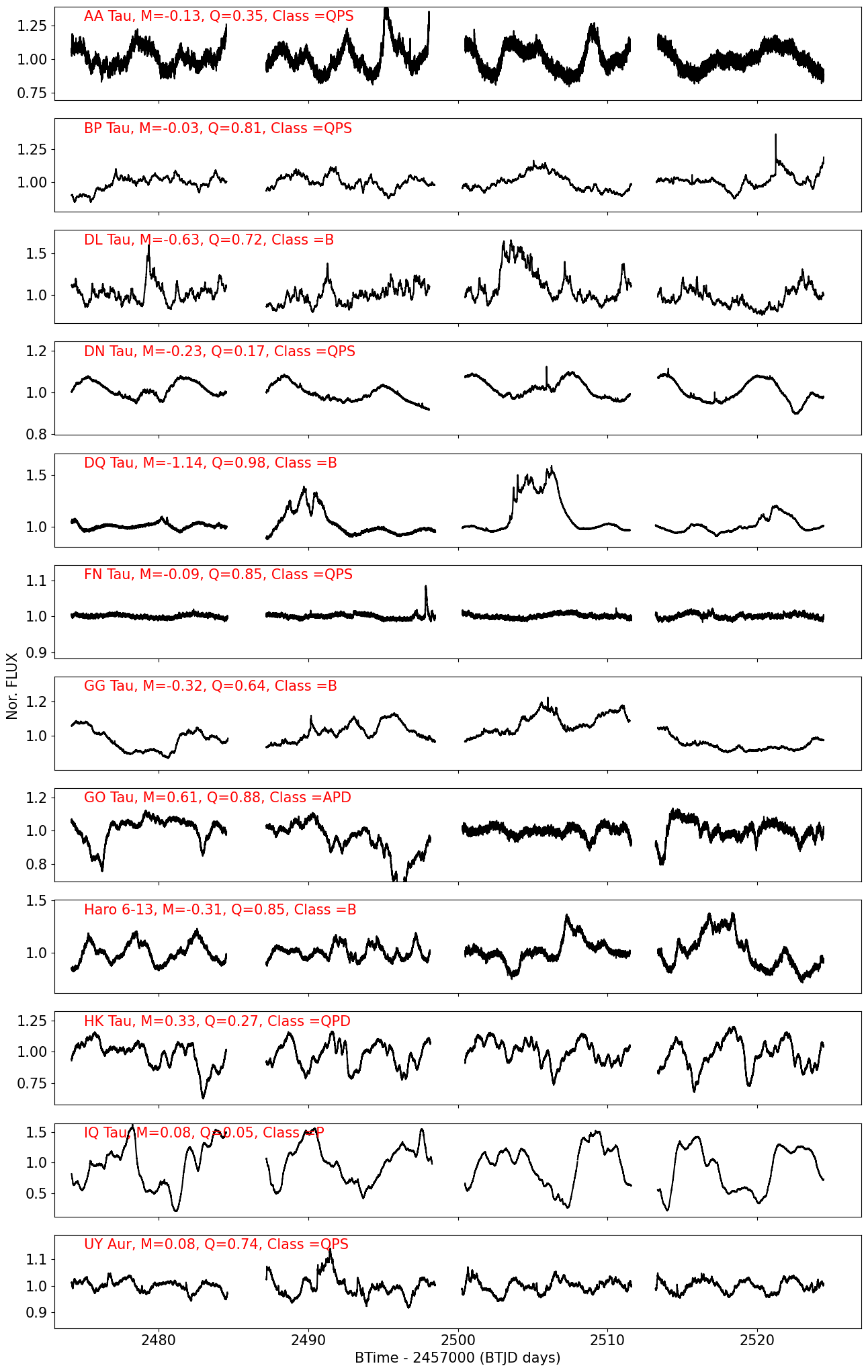
Figure 9: The TESS light curves of 12 CTTSs in our sample. Their variability classes are also displayed.

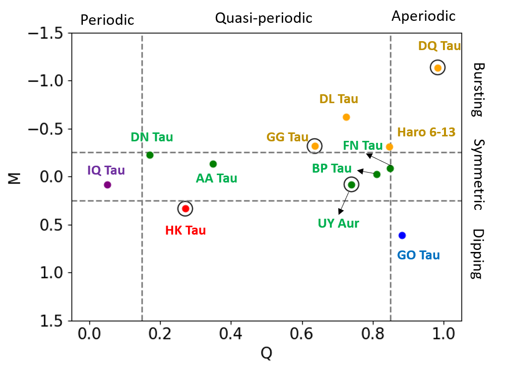
Figure 10: The $Q$–$M$ statistics diagram for our sample of CTTSs. The stars surrounded by black hollow circles in this diagram are binary or multi–star systems. Different colors represent different variability classes: yellow (B), purple (P), green (QPS), blue (APD), and red (QPD).

The values of Q and M for the CTTSs are listed in Table 4, along with the variability classes. The TESS light curves of 12 CTTSs in our sample, along with their assigned M, Q and variability classes, are shown in Figure 9. Also in Figure 10, we show the distribution of the variability statistics for our sample in the $Q$–$M$ diagram.

3.4 Mass–accretion rate measurements from TESS light curves

In Section 3.3, we have identified four bursters in our samples: DQ Tau, DL Tau, GG Tau, and Haro 6–13. To estimate the mass–accretion rates from their TESS light curves, we need to first convert the excess flux yields associated with the bursts in the $TESS$ bandpass to the U–band excess luminosity which can be used as the proxy for the mass–accretion rates (e.g., Tofflemire et al., 2017).

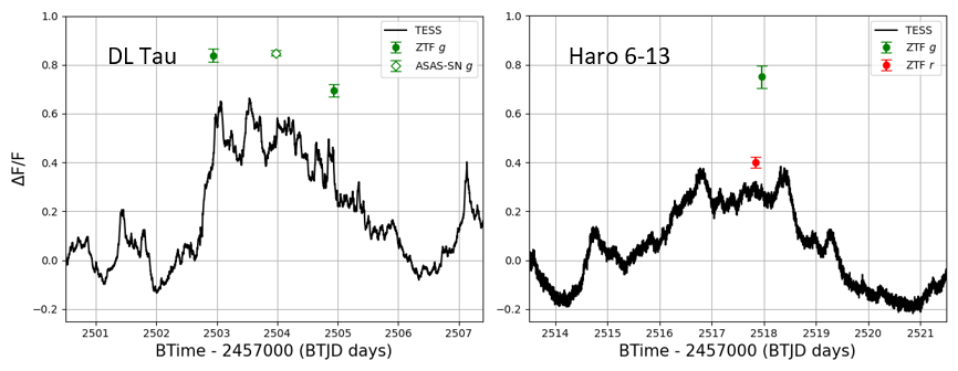
Figure 11: Left panel: A burst event of DL Tau at BT-2457000 = 2504 was captured by TESS, ASAS–SN $g$, and ZTF $g$. Right panel: A burst event of Haro 6–13 at BT-2457000 = 2516 was observed by TESS, ZTF $g$, and ZTF $r$. In each panel, the black curve represents the burst event observed by TESS, and the green filled circles are $g$ band observations from the ZTF survey. The hollow green diamond represents the data from the ASAS–SN survey. In the case of Haro 6–13, the red filled circle represents the observation from the ZTF $r$ band.

To do so, we searched for other observational data of the stars from ASAS-SN, Pan–STARRS, and ZTF (Bellm et al., 2019; Masci et al., 2019; IRSA, 2022), that were taken simultaneously with TESS in different optical bands. We found such data only for DL Tau and Haro 6–13. DL Tau was observed by the ASAS–SN survey and the ZTF survey. A burst event of DL Tau at BT-2457000 = 2504 days was captured by TESS, ZTF $g$, and ASAS–SN $g$. Haro 6–13 was observed by ZTF during the same observation period as the TESS mission for it. A burst event in Haro –13’s TESS light curve at BT-2457000 = 2516 days was also observed by the ZTF with both the $g$ and $r$ bands. Their light curves of the bursts are shown together in Figure 11.

Here, the periodic variation due to possible dark spot modulation has been removed from the TESS light curves of DL Tau and Haro 6–13 by subtracting the best–fit sinusoidal curves with corresponding periods (see Table 4) from the original curves. The fluxes of both data have good quality flags, and both are normalized to their respective median flux levels using the equation:

$$\frac{\Delta F}{\widetilde{F}}=\frac{F-\widetilde{F}}{\widetilde{F}},$$ (8)

where $F$ represents the flux as a function of time and $\widetilde{F}$ is their median in the light curve. We express the observed amplitude due to the hot spot associated with the accretion burst, that covers an area $A=X\pi R_{*}^{2}$ on the visible stellar photosphere, where $X$ is the filling factor and $R_{*}$ is the stellar radius as:

$$\left(\frac{\Delta F}{\widetilde{F}}\right)_{\lambda}=X\frac{\int B_{\lambda}(T_{\text{hspot}})R_{\lambda}d\lambda}{\int B_{\lambda}(T_{*})R_{\lambda}d\lambda}=X\frac{T_{\text{hspot}}^{4}f_{\lambda}(T_{\text{hspot}})}{T_{*}^{4}f_{\lambda}(T_{*})},$$ (9)

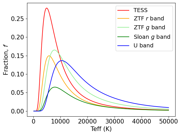
Figure 12: The fractional response functions of $TESS$ (red), ZTF $r$ (orange), ZTF $g$ (lightgreen), sdss $g$ (green), and $U$ bands (blue). They are the function of the blackbody temperature.

where $B_{\lambda}$ is the Planck function, $R_{\lambda}$ is the transmission function of the band, $T_{*}$ is the stellar effective temperature, and $T_{hspot}$ is the temperature of the hot spot. The integral term can be expressed as $\sigma T^{4}f_{\lambda}(T)$ where $\sigma$ is the Stefan–Boltzmann constant and $f_{\lambda}$ is the bandpass response factor as a function of temperature for the used band ($\lambda$). The response factor functions of the bands used in the study, i.e., sdss $g$, ZTF $g$, ZTF $r$, $U$, and $TESS$ bands, are shown in Figure 12. The amplitudes of DL Tau’s event are 0.848, 0.77, and 0.438 in ASAS-SN’s sdss $g$, ZTF $g$, and $TESS$ bands, respectively. We note that since there are two data points from ZTF $g$ obtained during the event, the reported amplitude in ZTF $g$ is computed as the mean value of these data points. Additionally, the central time between these two data points is very close to that of the ASAS-SN’s observation. With this information, we can estimate the temperature of the hot spot by using the following equation:

$$\frac{(\Delta F/\widetilde{F})_{\lambda 1}}{(\Delta F/\widetilde{F})_{\lambda 2}}=\frac{f_{\lambda 1}(T_{\text{hspot}})f_{\lambda 2}(T_{*})}{f_{\lambda 2}(T_{\text{hspot}})f_{\lambda 1}(T_{*})}.$$ (10)

The hot spot’s temperatures derived from $TESS$–ASAS-SN $g$ and $TESS$–ZTF $g$ are about 5700 K and 5500 K, respectively. As a result, the temperature of the hot spot is estimated to be the average of these values, which is approximately 5600 K. We substitute this value back to the Eq. 9 to calculate the filling factor of the spot and obtain $X=0.038$ or $3.8\%$.

For the case of Haro 6–13, the burst amplitudes in TESS, ZTF $r$, and ZTF $g$ bands are measured to be 0.292, 0.4, and 0.75, respectively. Because there is approximately a 0.1 day timing gap between the ZTF $g$ and ZTF $r$ data, the amplitude in the TESS band is the average of the corresponding amplitudes at ZTF $g$ and ZTF $r$ data times. By following the same estimation procedure as we conducted for DL Tau’s burst, the temperature of Haro 6–13’s burst is estimated to be 7100 K based on TESS and ZTF $g$ bands data. The estimated temperature becomes a bit hotter when using TESS and ZTF $r$ bands data, which is 7715 K. Thus we determined the burst temperature of Haro 6–13 to be about 7300 K by averaging these values. The filling factor of the burst–driven hot spot on Haro 6–13 is about $X=0.008$ or $0.8\%$. The resulting values of the hot spot temperature and fractional area fall within the range of values observed and modeled in previous studies (e.g., Manara et al., 2013; Venuti et al., 2015), demonstrating the reliability of our method. However, we note that our estimations are lower limits as we haven’t considered the limb–darkening in Eq. 9 and Eq. 10. In other words, we assume the hot spot is located at the center of the visible photospheric disk of the star.

We then extrapolate the burst amplitudes in the $U$–band with the estimated hot spot temperatures and the fractional areas. We find that the burst amplitudes in the $U$–band are about 3.49 times and 7.6 times higher than that in the $TESS$ band for DL Tau and Haro 6–13, respectively. We produce the $U$–band excess amplitude curves of DL Tau and Haro 6–13 by multiplying their normalized TESS light curves with the factors of counterparts. The U–band apparent magnitudes of DL Tau and Haro 6–13 are $14.04$ (Ducati, 2002) and $19.22$ (Audard et al., 2007), which can be converted to a flux unit of $F_{U}=3.77\times 10^{-11}erg~{}s^{-1}cm^{-2}$ and $F_{U}=3.19\times 10^{-13}erg~{}s^{-1}cm^{-2}$, respectively. The U–band luminosities, $L_{U}=1.15\times 10^{32}erg~{}s^{-1}$ and $L_{U}=6.32\times 10^{29}erg~{}s^{-1}$, of DL Tau and Haro 6–13 can be estimated using the formula $L_{U}=F_{U}4\pi d^{2}$ with the distance information of $d=159$ pc and $d=129$ pc (Gaia Collaboration, 2020). We produce the U–band excess luminosity ($L_{Uexcess}$) curves of these stars by multiplying their U–band excess amplitude curves with the $L_{U}$ values. Then the accretion luminosities ($L_{acc}$) can be calculated using an empirical correlation between $L_{acc}$ and $L_{Uexcess}$ given by Gullbring et al. (1998):

$$log(L_{acc}/L_{\odot})=1.09log(L_{Uexcess}/L_{\odot})+0.98,$$ (11)

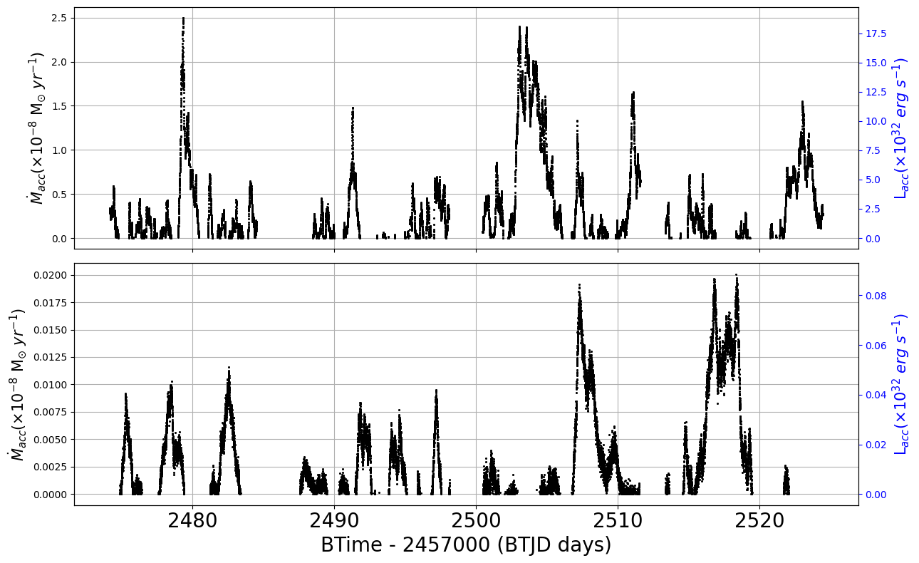
Figure 13: The time series mass–accretion rates of DL Tau and Haro 6–13 are shown in the upper panel and bottom panel, respectively. The left axis shows the mass–accretion rates derived from the TESS, ASAS–SN, and ZTF observations, while the right axis displays the corresponding accretion luminosities.

where $L_{\odot}$ is solar luminosity. Finally, the mass–accretion rates can be determined from the accretion luminosities by using Eq 6 with the stellar parameters in Table 2. The mass–accretion rates and luminosities of DL Tau and Haro 6–13 are displayed in Figure 13.

4 Results and Discussion

4.1 Mass–accretion rates from the LAMOST Spectra

We estimated the mass-accretion rates of low-mass classical T Tauri stars with spectral types from mid-M to late-K in the Taurus Molecular Cloud using LAMOST spectral data. The indicators we used were the H$\alpha$ 6563 $\AA$, H$\beta$ 4861 $\AA$, Ca$\text{II}$ 8498, 8542, 8662 $\AA$, and He$\text{I}$ 4471, 5875, 6678, 7065 $\AA$ emissions. The equivalent widths of these lines and the corresponding mass-accretion rates are listed in Table 5 and Table 6, respectively.

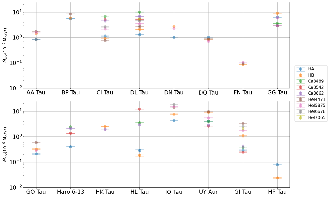
Figure 14: The distribution of mass-accretion rates derived from all available emissions in the spectra of our CTTSs. The names of the stars marked with an asterisk (*) in the upper right indicate that they are binary or multi–star systems.

All of our samples have the $\dot{M}_{acc}$ measurement estimated from H$\alpha$ line. On average, these stars have an H$\alpha$ mass–accretion rate of $1.76\times 10^{-9}M_{\odot}yr^{-1}$. GG Tau has the highest measured H$\alpha$ mass–accretion rate among the sample, with a value of $6.35\times 10^{-9}M_{\odot}yr^{-1}$. HP Tau has a significant H$\alpha$ emission, but its mass–accretion rate is lower than those of the other stars with a value of $7.88\times 10^{-11}M_{\odot}yr^{-1}$ in this study. On the other hand, from H$\beta$ emissions, the average rate of these star is $2.89\times 10^{-9}M_{\odot}yr^{-1}$. UY Aur and GG Tau both have the highest H$\beta$–derived rate of $9.11\times 10^{-9}M_{\odot}yr^{-1}$. Consistent with the H$\alpha$ result, HP Tau exhibits the lowest mass–accretion rate estimated from the H$\beta$ line, which is $2.44\times 10^{-11}M_{\odot}yr^{-1}$. Only Haro 6–13 has no H$\beta$ accretion rate because it is too faint for LAMOST in the blue wavelength part, making it impossible to estimate. Not all targets in our sample have measurable equivalent widths for the other emission lines, which means that not all corresponding mass–accretion rates could be estimated. Figure 14 shows the mass-accretion rate distribution of our targets by displaying the measurements derived from all available emissions adopted in this study. HL Tau has the largest dispersion of the spectral-derived mass-accretion rates with a coefficient of variation (CV) value (the ratio of the standard deviation to the mean) of $1.15$, as compared to other stars in the sample. The CVs of other stars are smaller than one with a mean value of 0.41$\pm$0.22. After field checking, we have ruled out the possibility of contamination from the closest neighboring star of HL Tau, XZ Tau, as it is located about $23^{\prime\prime}$ away from HL Tau, and thus, can be resolved separately by the LAMOST fiber with a $3.3^{\prime\prime}$ diameter. The underlying mechanism responsible for this phenomenon remains unknown, making it an intriguing topic for future investigation. On the other hand, the lowest dispersion CV value is found in FN Tau, which is $0.08$.

4.2 Mass–accretion rates of DL Tau and Haro 6–13 from the TESS light curves

The time–series mass accretions rates and luminosities derived from the TESS light curves for DL Tau and Haro 6–13 are shown in Figure 13. We find that the mass–accretion rate of DL Tau reached up to $2.5\times 10^{-8}M_{\odot}yr^{-1}$ during the observation time. The mass accreted by DL Tau over approximately 50 days is $\approx 3.4\times 10^{-10}M_{\odot}$, with an average rate of $\approx 2.5\times 10^{-9}M_{\odot}yr^{-1}$. These results are comparable to the mean value of the mass–accretion derived from LAMOST for DL Tau, which is $4.6\times 10^{-9}M_{\odot}yr^{-1}$ with a standard deviation of $2.5\times 10^{-9}M_{\odot}yr^{-1}$. Meanwhile, the maximum mass–accretion rate of Haro 6–13 from the TESS observations is $2\times 10^{-10}M_{\odot}yr^{-1}$. It accreted mass with a value of about $2.7\times 10^{-12}M_{\odot}$ over approximately 50 days, with an average rate of $\approx 2\times 10^{-11}M_{\odot}yr^{-1}$. These results are overall lower than the measurement, which is about $1.6\pm 0.8\times 10^{-9}M_{\odot}yr^{-1}$ on average, determined from LAMOST data.

An interesting question is whether the mass increase of T Tauri stars is dominated by long–term, steady mass accretion or by occasional bursts of accretion? First, we need to define a steady accretion rate, and this rate does not change over time. We then calculate the total mass accumulated by the steady rate of the star during the TESS observation. This is compared with the total amount of burst accretion to determine whether the CTTS is dominated by steady status or episodic effect.

Here, we take the mean rate obtained from LAMOST emission measurement as the steady rate. Thus, the steady rate of mass–accretion of DL Tau is $4.6\pm 2.5\times 10^{-9}M_{\odot}yr^{-1}$. In this case, DL Tau accumulated masses of $6.3\pm 3.4\times 10^{-9}M_{\odot}$ through steady rate over a period of about 50 days. This result is larger than the total mass of $\approx 3.4\times 10^{-10}M_{\odot}$ accreted by the stars’ burst–like events observed by TESS. Similarly, the steady mass–accretion of Haro 6–13 is $1.6\pm 0.8\times 10^{-9}M_{\odot}yr^{-1}$. This value is about one order higher than the maximum of $2\times 10^{-10}M_{\odot}yr^{-1}$ from the TESS observation. Therefore, in this scenario, the mass–accretion processes of DL Tau and Haro 6–13 are both steady accretion dominant.

4.3 Flare activity of our CTTSs sample

CTTSs are also known for their high magnetic activity, which is often manifested in flaring events. Flares with the sudden, short–lived increases in brightness are thought to be caused by magnetic reconnection events on the star’s surface (Parker, 1963; Maehara et al., 2012). The magnetic fields of the CTTS form a large loop connecting the star and circumstellar disk. When the magnetic field lines eventually reconnect, a large amount of energy is released in the form of a huge flare. This kind of the flare resulting from the star–disk magnetic interaction could last more than 50,000 seconds, and it is a characteristic feature of CTTS while affecting the mass–accretion process in some degree (Giardino et al., 2007; López-Santiago et al., 2016; Colombo et al., 2019).

4.3.1 Flare detection

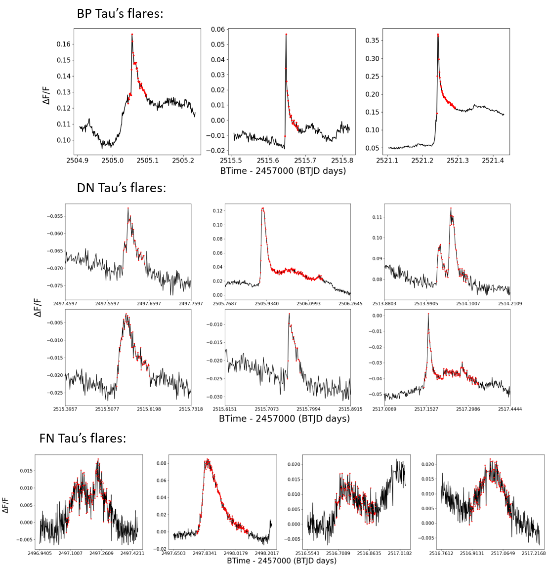
Figure 15: The profiles of 13 flare events detected in the Section 43 and 44 TESS light curves of BP Tau (3 flares), DN Tau (6 flares), and FN Tau (4 flares).

To analyze the flares in our TESS light curves, we employ an algorithm developed by Lin et al. (2019) that generates a flare–free light curve. We then identify individual flare candidates from a residual curve generated by subtracting the flare–free light curve from the original curve. This method allows us to accurately quantify the properties of each flare, including its amplitude, duration, and energy release. We further examine the candidates for their authenticity by visually inspecting the Target Pixel File to generate the light curve of each pixel, using the Python package Lightkurve (Lightkurve Collaboration et al., 2018) and the method described by Wu et al. (2015). In our sample, we detect flares in the light curves of three stars: BP Tau (3 flares), DN Tau (6 flares), and FN Tau (4 flares), in total 13 flares, and some of them are multi–flare events. The light curve profiles of these flares are shown in Figure 15. However, the absence of flares in other stars does not necessarily mean that they are not flaring stars. For example, Tofflemire et al. (2017) and Kóspál et al. (2018) both detected several flare events in DQ Tau from optical and Kepler observations, whereas we did not detect any flares in DQ Tau from the TESS observation in this study. It is possible that there are microflares with amplitudes or duration that are too small to be detected by TESS.

4.3.2 Flare amplitude and energy

The amplitude of the flare profile as a function of time can be determined using the Eq. 8. The flare energy is estimated using an equivalent duration (ED) method defined as follows (Gershberg, 1972):

$$\mathnormal{ED=\int\frac{\Delta F(t)}{\widetilde{F}}dt.}$$ (12)

It represents the time it takes for a non-flaring star to emit the same amount of energy as that released during a given flare. Therefore, this quantity can be used to estimate the energy of the flare by multiplying it by the quiescent stellar flux in the telescope bandpass

$$\mathnormal{E_{f,\lambda}=ED\times F_{*,\lambda},}$$ (13)

and the corresponding quiescent stellar flux of the star can be estimated from

$$\mathnormal{F_{*,\lambda}=4\pi R_{*}^{2}\sigma T_{*}^{4}f_{\lambda}(T_{*}).}$$ (14)

Here, $R_{*}$ is the stellar radius, $T_{*}$ is the effective temperature, and $\sigma$ is the Stefan–Boltzmann constant. $f_{\lambda}$ is the same function as appeared firstly in Eq. 9, which is a bandpass response factor as a function of temperature for the wavelength ($\lambda$) band and in this case $\lambda=TESS$, i.e., the fractional response function of TESS (see Figure 12).

The amplitudes, duration, timing at peak in BTJD, and released energy of detected flares are listed in Table 7. These flares have energy levels ranging from $2\times 10^{34}$ erg to $6\times 10^{35}~{}$erg. The flare with the highest amplitude of 0.22 is observed in BP Tau, with a duration of about 76 minutes and energy of $1\times 10^{35}$erg. The most energetic flare in our sample is observed in FN Tau, with an energy of $6.3\times 10^{35}$ erg, an amplitude of 0.09, and a duration of 438 minutes. Furthermore, given the duration of the flares, these events likely originate from the localized magnetic reconnections near the stellar surface.

4.3.3 Flare frequency distribution

The flare activity of a star can be characterized by its flare frequency distribution, which can be described by a linear relationship expressed in logarithmic form as

$$\mathnormal{log~{}N=a+\beta~{}log~{}E,}$$ (15)

where $N$ is the cumulative frequency of flares with released energy $E$. The slope of the distribution, represented by the coefficient $\beta$, can provide information about the properties of the star’s flare activity. If $\beta<$-1, then most of the total energy emitted by the flares comes from small flares, while for $\beta>$-1, stronger flares dominate the energy output. The flare frequency distribution power–law can also be expressed in differential form as

$$\mathnormal{dN\propto E^{-\alpha}dE,}$$ (16)

where $dN$ is the number of flares with energies in the range of $E$ and $E+dE$, and $\alpha=1-\beta$ (Hawley et al., 2014). We use the maximum likelihood estimator (MLE) for $\alpha$ as derived by Clauset et al. (2009):

$$\mathnormal{\alpha=1+n\left[\sum^{n}_{i=1}\ln\frac{E_{i}}{E_{min}}\right]^{-1},}$$ (17)

and the error for $\alpha$ can be estimated from

$$\mathnormal{\sigma_{\alpha}=\frac{\sqrt{n+1}(\alpha-1)}{n}.}$$ (18)

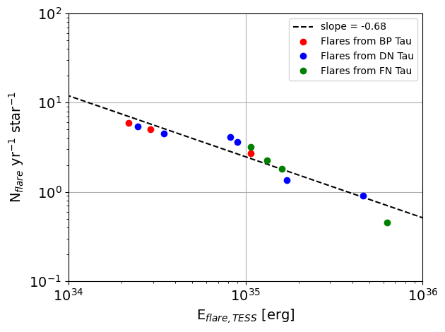
Figure 16: The flare frequency distribution and the best–fits power–law function with a slope of -0.68$\pm$0.20 of our CTTS sample based on 13 detected flares in this study.

Here, $n$ is the number of flare samples, and $E_{min}$ is the minimum value of the energy of the observed flares. By setting $E_{min}=2.2\times 10^{34}$ erg and $n=13$, we have calculated the value of $\alpha$ to be $1.68\pm 0.20$. From this, we can derive the linear slope of logarithmic flare frequency distribution, which is represented by $\beta=-0.68\pm 0.20$ and a constant $a$ of $24.32$. Figure 16 shows the flare frequency distribution and its best–fit power–law slope for our CTTS sample. These results suggest that strong flares with high energy dominate the flare activity of these stars. The power–law distribution also indicates that our sample stars exhibit extreme flare activity, with the ability to generate flares with energy levels stronger than $E=1\times 10^{34}$ erg about 12 times per year. This is in stark contrast to solar-type stars, which produce flares of this magnitude only once every 35–40 years (Shibayama et al., 2013). Even one of the most flare–active young M stars, Wolf 359, can produce only one such flare a year (Lin et al., 2021).

4.4 The changes of the variability classes

The changes in the variability behavior of the CTTSs can be attributed as the inner disk structure responsible for the stellar occultation, which can undergo significant changes in just a few years, transitioning from a stable and well-organized geometry with a consistent inner disk warp to a more disordered distribution of dust (e.g., McGinnis et al., 2015). Another explanation is the stability of the accretion regime. Initially, the accretion geometry may consist of a main accretion funnel in each hemisphere, with the base of each funnel corresponding to the stable inner disk warp. However, over time, this geometry may become unstable, resulting in the formation of random accretion funnels (e.g., Kurosawa & Romanova, 2013). Cold spots due to the strong magnetic field of CTTSs might be able to cover a large fraction of stellar surface, which is similar to magnetically active low–mass stars (e.g., Yang et al., 2017; Lin et al., 2021), and the changes of their distribution and sizes may be also reflected in the changes of variability behaviors (e.g., Frasca et al., 2005).

Ten stars in our sample were previously observed by K2 Campagin 13 (AA Tau, DQ Tau, GO Tau, Haro 6–13 HK Tau, HL Tau, and IQ Tau), or TESS Section 19 (BP Tau, FN Tau, and UY Aur), and their light curves were analyzed and classified for variability by Cody et al. (2022) and Robinson et al. (2022). The variability classes given by Cody et al. (2022) and Robinson et al. (2022) are also listed in Table 4. By comparing the variability classes given by Cody et al. (2022) based on the K2 C13 data observed about four years ago, we find that most of the stars (6 out of 7) change their variability classes except DQ Tau. Specifically, AA Tau changes from ”S” to ”QPS”, GO Tau changes from ”U” to ”APD”, Haro 6–13 changes from ”S” to ”B”, HK Tau changes from ”QPS” to ”QPD”, IQ Tau changes from ”QPS” to ”P”, and HL Tau changes from ”QPS” to ”QPD”. In contrast, the variability classes of BP Tau and FN Tau do not change compared to those derived by Robinson et al. (2022) using TESS Section 19 light curves from about 600 days ago. Even though UY Aur changes from ”B” to ”QPS” in 600 days, we still see a burst–like event at BJTD $=$ 2491 in its TESS Section 43 light curve. These findings may suggest that the long–term timescale of the variation associated with, for example, the stable/unstable accretion regime and inner disc warp due to the star–disk interaction of the CTTSs is in the range between about 1.6 years to 4 years or longer. However, it remains to be determined whether these changes occur in a cyclical or random manner. For instance, Haro 6–13 changing from the ”B” type back to the ”S” type, or to any other type, would require further investigation through continuous monitoring in the future.

4.5 Effect of the inclination on the spectra, accretion, and variability properties

The spectral properties of the CTTSs have been predicted to be correlated with the inclination of the system, especially with the broad or high–velocity component of the forbidden line profile (e.g., Hartigan et al., 1995). The high-velocity components are generally believed to originate in fast outflows that keep thrusting material into interstellar space in form of jets. Among the known forbidden lines, the ones with the most distinctive high–velocity component spectral features are the [NII] lines at 6548 $\AA$ and 6583 $\AA$, which behave as blueshifted emission with a well-defined peak (Hirth et al., 1997). Nevertheless, the resolving power of the LAMOST observations is not high enough to distinguish the [NII] lines from H$\alpha$ emission, thus we can not derive the outflow velocity from these lines using the data we have in this study.

Additional forbidden lines that can provide insight into the wind velocity observed by LAMOST are the [OI] line at 6300 $\AA$, [SII] lines at 6716 $\AA$ and 6731 $\AA$, and [CaII] lines at 7291 $\AA$ and 7323 $\AA$. While the blueshifted emission of the [OI] line may not display a distinct peak when compared to the [NII], [SII], and [CaII] lines, the extended blue wing can be interpreted as an indicator of the projected wind velocity (Appenzeller & Bertout, 2013). Out of the sample CTTSs, ten stars exhibit [OI] lines in their LAMOST spectra, while [SII] lines have only been detected in AA Tau and HL Tau. Moreover, [CaII] lines are observed in only one star, HL Tau.

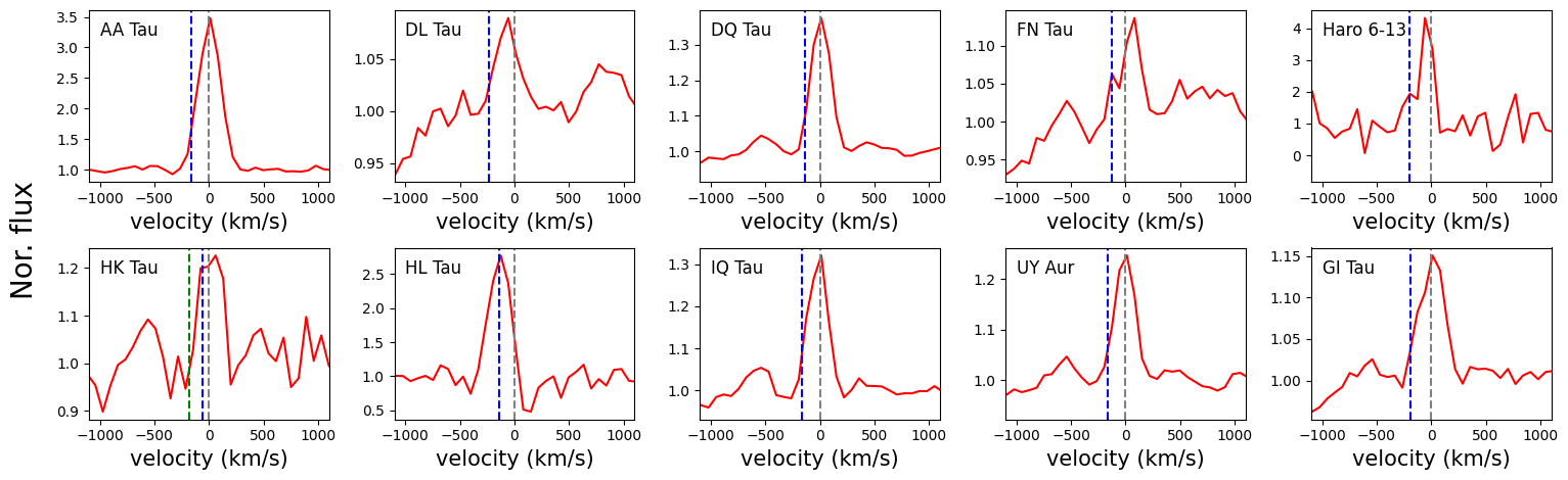
Figure 17: The velocity profiles of [OI] 6300 lines of ten CTTSs in our sample. In each panel, the gray vertical dashed line indicates the center of the line, and blue dashed line marks the wind velocity of the blueshifted wind or peak of the line. In a special case of HK Tau, we also show a green dashed line to represent the blueshifted wind velocity, which is likely originating from a companion of the binary system, HK Tau A, and the blueshifted peak velocity marked with a blue dashed line belongs to the other companion of the system, HK Tau B.

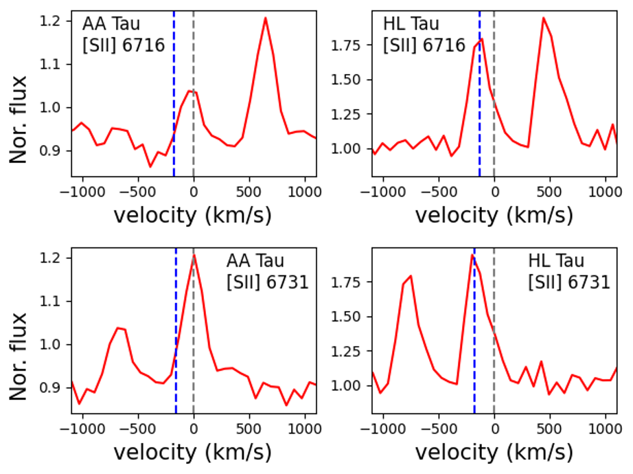
Figure 18: The velocity profiles of [SII] lines observed in the spectra of AA Tau and HL Tau. In each panel, the gray vertical dashed line indicates the center of the line, and blue dashed line marks the wind velocity of the blueshifted wind or peak of the line.

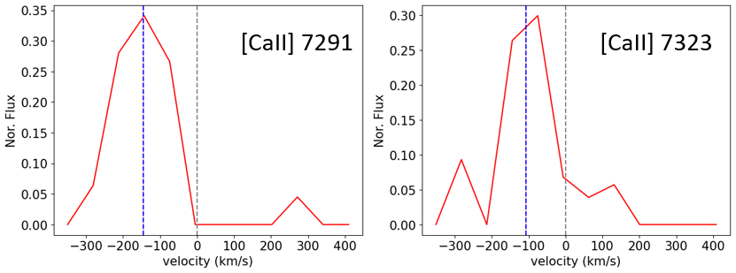
Figure 19: The velocity profiles of [CaII] lines of HL Tau. The gray vertical dashed line indicates the center of the line, and blue dashed line marks the wind velocity of the blueshifted peak of the line.

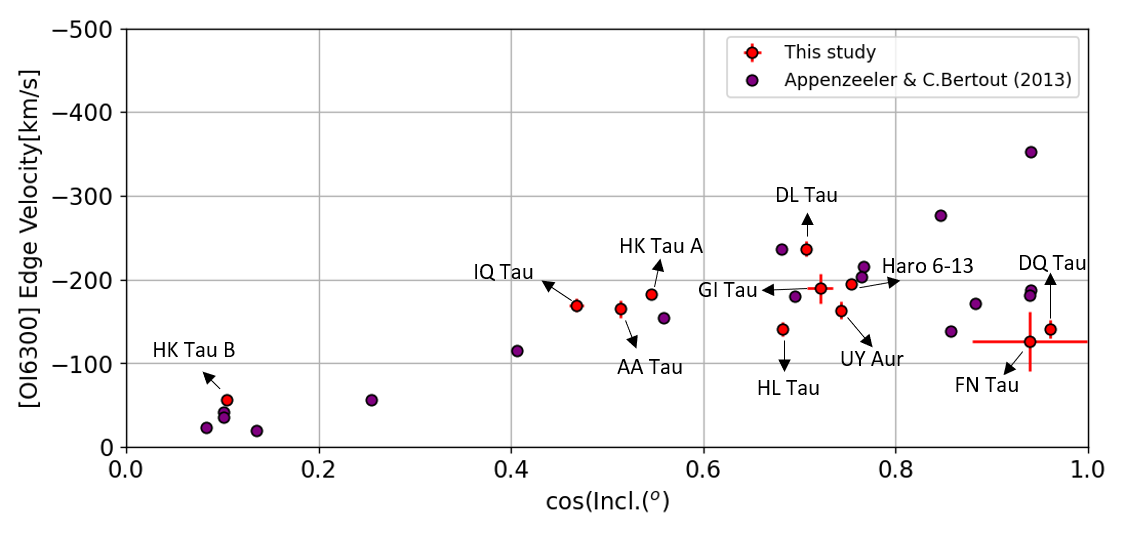
Figure 20: The comparison between CTTSs’ OI 6300 project wind velocities (vertical axis) and inclinations in terms of cosine angle (horizontal axis). The purple circles represent the data from Appenzeller & Bertout (2013), and the red circles are the data in this study.

We estimate the projected wind velocity by using the blue edge of the line profile with flux reaching 25$\%$ of the peak value when the line shows no clear blue peak. Because of the low resolution of the LAMOST data, for those profiles showing a blue peak, the velocity is directly estimated from the wavelength of the peak. The LAMOST [OI] line, [SII] lines, and [CaII] lines velocity profiles of the CTTSs are shown in Figure 17, Figure 18, and Figure 19, respectively. The results of [OI], [SII], and [CaII] velocity measurements are listed in Table 8. For stars where velocity measurements are available from not only [OI], but also [SII] and [CaII], i.e., AA Tau and HL Tau, the results are consistent across all lines. We note that there are two [OI] velocity results for a binary HK Tau. The diameter of LAMOST’s fiber is about 3.3 arcsecond, and the angular separation between HK Tau A and HK Tau B is about 2.3 arcsecond. Thus, LAMOST observation can not resolve these two stars separately. We detect a blueshifted peak of [OI] line at a wind velocity of $-56.49$ km/s, which may have originated from the edge–on system HK Tau B with an inclination of $84^{o}$. The velocity derived from the blue edge of the line with a value of $-182.88$ km/s belongs to HK Tau A, which has a relatively face–on disk with an inclination of $i=56.9^{o}$. The comparison between the inclinations and [OI] line-derived projected wind velocity is shown in Figure 20. Our results show a positive correlation between the cosine of inclination and the projected wind velocity, consistent with the trend observed by Appenzeller & Bertout (2013).

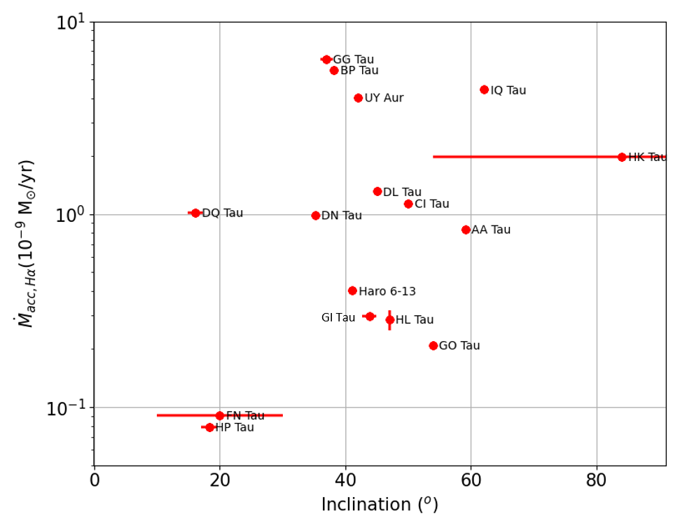
Figure 21: The relationship between the inclination and mass–accretion rates derived from the H$\alpha$ emission luminosities. The Pearson’s correlation coefficient is about 0.34, indicating the correlation is not significant.

The inclination angle of a CTTS may have an impact on the estimation of its mass–accretion rate to some degree. This is because the varying geometric angle of the disk could obscure areas emitting accretion–associated emission from the line of sight, leading to uncertainties in the measurement. However, our analysis indicates that there is no significant correlation between the inclination angle and the log spectra–derived mass–accretion rates (see Figure 21) with a Pearson’s correlation coefficient of 0.34 for H$\alpha$’s measurement, and the correlation coefficients are even lower for the results from other emissions. One possibility is that the emission regions driven by accretion are uniformly distributed on the surface of the CTTS, making the effect of disk obscuration negligible. Another possible explanation is that the properties of the inner disk may play a more significant role than those of the outer disk. Several studies have reported misalignments between the inner and outer disks. For example, the inner disk of AA Tau has an inclination angle of $i=75$ deg, closer to edge-on (Bouvier et al., 2003; O’Sullivan et al., 2005), while the outer disk has an inclination angle of $i=59$ deg (Loomis et al., 2017). Unfortunately, information on the inclination angle of the inner disk for our sample stars, except for AA Tau, is not available. Further studies using high–resolution double–peaked Keplerian line spectroscopic observations or spatially resolved observations using infrared interferometry on VLTI may be required to address this issue.

The type of photometric variability of CTTS is dominated by the accretion and dark spots located on the photosphere and the disk around, thus it could be geometric viewing angle dependent. Cody & Hillenbrand (2018) found a positive correlation between the M value they estimated and the inclination Barenfeld et al. (2017) gave, so that dippers and QPS sources tend to have high inclinations, while bursters and stochastic sources have low inclinations. However, due to the substantial uncertainties associated with the inclination measurements, they cautiously stated this observed tendency. A more recent study by Robinson et al. (2022), based on CTTSs with lower inclination uncertainties, found little evidence for a strong correlation between disk inclination and M value (see Fig.12 in their paper). The upper panel shown in Figure 22 illustrates the relationship between inclination and M value of CTTS, including our samples and those from Robinson et al. (2022). Our analysis reveals a relatively strong and positive correlation between M value and inclination, with a Pearson’s value of $0.61\pm 0.03$, compared to the results given by Cody & Hillenbrand (2018) and Robinson et al. (2022).

On the other hand, we find an indistinct and negative correlation between the periodicity metric Q value and inclination with a Pearson’s value of $-0.54\pm 0.03$ (see the bottom panel in Figure 22) for our targets. This is consistent with the conclusion given by Robinson et al. (2022) who also found the weak inverse correlation between disk inclination and periodicity metric of Taurus CTTSs. Furthermore, the distribution of variability classes in the inclination–Q space in our study is similar to that of Taurus members studied by Cody et al. (2022), as shown in Figure 7 of their paper. Nevertheless, it is possible that such distribution and the correlation between M value and inclination, as well as the correlation between periodicity metric Q value and inclination, could vary over time due to the changing variability classes of CTTSs.

5 Summary

We present a comprehensive study of 16 low–mass classical T Tauri stars in TMC for their mass–accretion and luminosity variability properties by using LAMOST low–resolution spectra and TESS photometric light curves.

From the LAMOST spectra, the mass–accretion rates of 16 CTTSs have been estimated using H$\alpha$, H$\beta$, Ca$\text{II}$, and He$\text{I}$ emissions as indicators. The average mass–accretion rate of all our samples based on H$\alpha$ lines is found to be $1.76\times 10^{-9}M_{\odot}yr^{-1}$. Not all targets in the sample have measurable equivalent widths for the other emission lines, which means that not all corresponding mass–accretion rates could be estimated. HL Tau has the largest dispersion of the spectral–derived mass-accretion rates with a coefficient of variation (CV) value of $1.15$, which is the ratio of the standard deviation to the mean. The reason that causes this huge dispersion remains unclear. On the other hand, the lowest dispersion CV value is found in FN Tau, which is $0.08$.

We also compute the time–series mass–accretion rates based on the TESS light curve, ZTF, and ASAS–SN survey for the stars DL Tau and Haro 6–13, which are identified to be the bursters according to their brightness variability asymmetry metric M values of $-0.63$ and $-0.31$, respectively (Cody et al., 2014). In total over about 50 days, the average accretion rates of DL Tau and Haro 6–13 are $2.5\times 10^{-9}M_{\odot}yr^{-1}$ and $1.4\times 10^{-11}M_{\odot}yr^{-1}$, respectively. The rate of DL Tau is consistent with the mean value of the mass–accretion derived from LAMOST. However, for Haro 6–13, this rate is generally lower compared to the LAMOST estimate We further investigate whether the mass–accretion mechanisms of these two stars are dominated by steady or burst accretion. By assuming the average rates obtained from LAMOST emission measurement as the steady rates, the mass accretions in DL Tau and Haro 6–13 are dominated by the steady process.

We have detected 13 flares in total in BP Tau, DN Tau, and FN Tau. The amplitude, duration, timing at peak in BTJD, and released energy of detected flares are determined, with the most energetic flare observed in FN Tau with the energy of $6.3\times 10^{35}$ erg. The power–law flare frequency distribution with a slope of $\beta=-0.68\pm 0.20$ indicates that the flare activity of the CTTSs is dominated by strong flare with high energy. Our analysis of the flare frequency distribution also reveals that the stars in our sample display extremely high levels of flare activity with the capability of producing flares with energy greater than $E=1\times 10^{34}$ erg up to 12 times per year, which is a significant deviation from solar–type stars and young M dwarfs.

Ten stars in our sample were previously observed and classified for variability by Cody et al. (2022) and Robinson et al. (2022). Comparing the variability classes from Cody et al. (2022) based on K2 Campaign 13 data from about four years ago, we found that most of the stars (6 out of 7) showed changes in their variability, except for DQ Tau. In comparison with the results from Robinson et al. (2022), BP Tau and FN Tau’s variability classes remained the same, while UY Aur changed from ”B” to ”QPS” in 600 days but still exhibited a burst–like event in its TESS Section 43 light curve. These findings suggest that the long-term timescale of variation in CTTSs could be between 1.6 to 4 years or longer and require further investigation to determine if changes occur cyclically or randomly.

The CTTSs’ projected wind velocities in terms of the blue edge/peaks of [OI], [SII], and [CaII] forbidden emissions detected in LAMOST are found to be correlated with the inclination, that is stars with low inclination tend to have fast projected wind velocity. On the other hand, no tendency has been found between inclination and mass–accretion rates derived from the spectral lines’ luminosities. One possibility is that the regions of emission driven by accretion are distributed uniformly across the stellar surface, so the disk obscuration doesn’t have much of an impact. Alternatively, it’s possible that the properties of the inner disk are more important than those of the outer disk. There is evidence to suggest that the inner and outer disks of CTTS can become misaligned due to, e.g., magnetic warping. Unfortunately, in our sample, only AA Tau has reported inner disk inclination angle. High–resolution double–peaked Keplerian line spectroscopic observations or spatially resolved observations using infrared interferometry on VLTI may be required for further studies of this topic.

The brightness variabilities of CTTSs have been also considered to be influenced by the inclinations to some degree. Our analysis reveals a relatively significant and positive correlation between M value and inclination, with a Pearson’s value of $0.61\pm 0.03$, compared to the results given by Cody & Hillenbrand (2018) and Robinson et al. (2022). We observed a weak negative correlation between the periodicity metric Q value and inclination for our targets, with a Pearson’s value of $-0.54\pm 0.03$. This finding supports the conclusion reached by Robinson et al. (2022), who also reported a weak inverse correlation between disk inclination and the periodicity metric of Taurus CTTSs. Additionally, we found that the distribution of variability classes in the inclination–Q space is similar to that of Taurus members studied by Cody et al. (2022). However, since the variability classes of CTTSs can change over time, it is possible that the distribution and correlations between the M value and inclination, and the periodicity metric Q value and inclination, could vary as well. Thus, further research is required to fully understand the long-term evolution of these correlations.

Table 1:
16 CTTSs in TMC observed by LAMOST and TESS.

	Name	LAMOST Obser. Date	TIC
	(1)	(2)	(3)
1	AA Tau	2019-01-29	268510757
2	BP Tau	2014-01-25	58287935
3	CI Tau	2016-02-07	61230756
4	DL Tau	2012-12-23	268444139
5	DN Tau	2012-12-23	268511247
6	DQ Tau	2020-01-26	436614017
7	FN Tau	2014-01-25	56625009
8	GG Tau	2016-02-05	245830955
9	GO Tau	2013-11-29	125914458
10	Haro 6-13	2012-12-23	268324608
11	HK Tau	2012-11-07	268324063
12	HL Tau	2013-02-09	353752575
13	IQ Tau	2012-12-23	268219495
14	UY Aur	2019-12-30	96205005
15	GI Tau	2019-01-29	268444803
16	HP Tau	2012-12-23	118521708

Table 2:
Stellar properties of 16 CTTSs in this study

Name	Radius	Mass	Spec. type	Distance	Inclination
	(R⊙)	(M⊙)		(pc)	(deg)
(1)	(2)	(3)	(4)	(5)	(6)
AA Tau	1.72	0.55	M0.6	134.671	59.1$\pm$0.3
BP Tau	1.30	0.63	M0.5	127.398	38.2$\pm$0.5
CI Tau	1.53	0.90	K5.5	160.318	50.0$\pm$0.3
DL Tau	1.20	0.94	K5.5	159.936	45.0$\pm$0.2
DN Tau	2.05	0.55	M0.3	128.601	35.2$\pm$0.5
DQ Tau	1.77	0.54	M0.6	195.381	16.1$\pm$1.2
FN Tau	2.30	0.29	M3.5	129.894	20.0$\pm$10.0
GG Tau	2.39	0.63	K7.5	116.395	37.0$\pm$1.0
GO Tau	1.25	0.41	M2.3	142.383	53.9$\pm$0.5
Haro 6-13	1.83	0.84	K5.5	128.555	41.1$\pm$0.3
HK Tau*	1.36	0.49	M1.5	140.000	56.9(HK Tau A), 84.0 (HK Tau B)
HL Tau	7.00	1.70	K3	140.000	47.0$\pm$0.4
IQ Tau	1.55	0.51	M1.1	131.511	62.1$\pm$0.5
UY Aur	1.90	0.70	K7.0	152.279	42.0
GI Tau	1.72	0.58	M0.4	129.436	43.8$\pm$1.1
HP Tau	1.81	1.06	K4.0	171.248	18.3$\pm$1.3

Table 3:
Photometric data of our samples taken by ASAS–SN and Pan–-STARRS surveys within 20 days of LAMOST observation.

	Name	LAMOST OBT	ASAS–SN OBT	ASAS–SN $g$	ASAS–SN $V$	Pan–Starrs OBT	Pan–Starrs $g$	Pan–Starrs $i$
		(MJD)	(MJD)	(mJy)	(mJy)	(MJD)	(mJy)	(mJy)
	(1)	(2)	(3)	(4)	(5)	(6)	(7)	(8)
1	AA Tau	58512.516	58512.037	0.88$\pm$0.06	…	…	…	…
2	BP Tau	56682.458	56700.294	…	48.58$\pm$0.18	…	…	…
3	CI Tau	56682.458	57424.345	…	16.49$\pm$0.14	…	…	…
4	DL Tau	56284.592	…	…	…	53600.366	10.37$\pm$0.01	…
5	DN Tau	56284.609	…	…	…	56333.298	26.09$\pm$0.02	…
6	GO Tau	56625.627	…	…	…	56605.593	…	47.64$\pm$0.06
7	Haro 6-13	56284.597	…	…	…	56300.366	1.25$\pm$0.01	…
8	HK Tau	56238.778	…	…	…	56236.566	…	52.60$\pm$0.06
9	HL Tau	56332.471	…	…	…	56333.325	1.57$\pm$0.01	…
10	IQ Tau	56284.607	…	…	…	56300.365	49.00$\pm$0.04	…

Table 4: The photometric variability classes of the CTTSs observed by TESS in this study and the literature (if any).

Name	M*	MC	MR	Q*	QC	QR	Variability*	VariabilityC	VariabilityR	Period∗	PeriodP	PeriodRe
(1)	(2)	(3)	(4)	(5)	(6)	(7)	(8)	(9)	(10)	(11)	(12)	(13)
AA Tau	-0.13	-0.30	…	0.35	1.00	…	QPS	S	…	8.3	8.2	…
BP Tau	-0.03	…	-0.03	0.81	…	0.83	QPS	…	QPS	7.6	7.6	…
DL Tau	-0.63	…	…	0.72	…	…	B	…	…	10.4	9.35	…
DN Tau	-0.23	…	…	0.17	…	…	QPS	…	…	6.18	6.1	…
DQ Tau	-1.14	-0.87	…	0.98	0.54	…	B	B	…	3.03	…	3.03
FN Tau	-0.09	…	0.03	0.85	…	0.60	QPS	…	QPS	7.33	…	8.77
GG Tau	-0.32	…	…	0.64	…	…	B	…	…	10.3	10.3	…
GO Tau	0.61	0.25	…	0.88	0.90	…	APD	U	…	2.51	…	…
Haro 6-13	-0.31	0.10	…	0.85	0.92	…	B	S	…	3.27	…	3.27
HK Tau	0.33	0.11	…	0.27	0.72	…	QPD	QPS	…	3.31	3.31	…
IQ Tau	0.08	-0.13	…	0.05	0.78	…	P	QPS	…	12.92	…	6.67
UY Aur	0.08	…	-0.49	0.74	…	0.74	QPS	…	B	3.04	…	…

=6.5cm

Table 5:
Equivalent widths of all mass–accretion indicator emissions of 16 CTTSs in LAMOST spectra in this study.

Name	$EW_{H\alpha}$				$EW_{H\beta}$				$EW_{Ca\text{II}8498}$				$EW_{Ca\text{II}8542}$				$EW_{Ca\text{II}8662}$		$EW_{He\text{I}4771}$	$EW_{He\text{I}5875}$	$EW_{He\text{I}6678}$	$EW_{He\text{I}7065}$
(1)	(2)				(3)				(4)				(5)				(6)		(7)	(8)	(9)	(10)
AA Tau	66.45	1.16 $\pm$	18.96	0.33	.	… $\pm$	.	…	.	… $\pm$	2.14	0.06	3.00	0.07 $\pm$	0.66	0.02	.	… $\pm$
BP Tau	98.29	0.06 $\pm$	23.15	0.01	.	… $\pm$	.	…	.	… $\pm$	2.98	0.05	.	… $\pm$	.	…	.	… $\pm$
CI Tau	44.39	2.07 $\pm$	13.18	0.61	11.74	0.10 $\pm$	10.18	0.06	8.68	0.01 $\pm$	0.96	0.02	2.17	0.06 $\pm$	0.73	0.04	.	… $\pm$
DL Tau	83.17	0.78 $\pm$	28.41	0.27	40.52	2.43 $\pm$	44.29	0.00	37.03	0.60 $\pm$	2.63	0.08	5.45	0.03 $\pm$	1.92	0.05	1.78	0.03 $\pm$
DN Tau	17.06	0.76 $\pm$	9.70	0.43	.	… $\pm$	.	…	.	… $\pm$	.	…	0.85	0.05 $\pm$	.	…	.	… $\pm$
DQ Tau	81.36	1.31 $\pm$	20.44	0.33	.	… $\pm$	.	…	.	… $\pm$	1.89	0.15	1.73	0.11 $\pm$	.	…	.	… $\pm$
FN Tau	22.36	0.53 $\pm$	11.57	0.27	.	… $\pm$	.	…	.	… $\pm$	0.82	0.00	1.34	0.03 $\pm$	.	…	.	… $\pm$
GG Tau	59.92	1.35 $\pm$	26.44	0.60	2.12	0.05 $\pm$	2.08	0.02	1.91	0.06 $\pm$	.	…	1.55	0.00 $\pm$	.	…	.	… $\pm$
GO Tau	36.64	2.01 $\pm$	20.68	1.13	.	… $\pm$	.	…	.	… $\pm$	2.74	0.06	1.73	0.13 $\pm$	.	…	.	… $\pm$
Haro 6-13	73.51	1.74 $\pm$	.	…	4.97	0.00 $\pm$	4.59	0.00	4.16	0.00 $\pm$	.	…	.	… $\pm$	.	…	.	… $\pm$
HK Tau	57.27	0.97 $\pm$	25.12	0.42	.	… $\pm$	.	…	.	… $\pm$	.	…	1.75	0.04 $\pm$	.	…	.	… $\pm$
HL Tau	59.73	10.95 $\pm$	10.67	1.96	27.57	0.60 $\pm$	28.72	0.00	24.13	0.29 $\pm$	.	…	.	… $\pm$	.	…	.	… $\pm$
IQ Tau	24.67	0.84 $\pm$	13.81	0.47	.	… $\pm$	.	…	.	… $\pm$	2.37	0.16	2.13	0.04 $\pm$	0.66	0.02	.	… $\pm$
UY Aur	46.27	0.97 $\pm$	16.32	0.34	3.36	0.07 $\pm$	2.74	0.05	2.74	0.00 $\pm$	1.43	0.06	1.42	0.04 $\pm$	.	…	.	… $\pm$
GI Tau	25.33	1.60 $\pm$	14.41	0.91	1.34	0.00 $\pm$	1.04	0.07	1.51	0.00 $\pm$	2.89	0.06	3.07	0.03 $\pm$	1.51	0.02	0.91	0.00 $\pm$
HP Tau	12.44	0.59 $\pm$	2.13	0.10	.	… $\pm$	.	…	.	… $\pm$	.	…	.	… $\pm$	.	…	.	… $\pm$

=6.5cm

Table 6:
Mass–accretion rates of 16 CTTSs derived from LAMOST spectra in this study.

Name	$\dot{M}_{H\alpha}$				$\dot{M}_{H\beta}$				$\dot{M}_{Ca\text{II}8498}$				$\dot{M}_{Ca\text{II}8542}$				$\dot{M}_{Ca\text{II}8662}$		$\dot{M}_{He\text{I}4771}$	$\dot{M}_{He\text{I}5875}$	$\dot{M}_{He\text{I}6678}$	$\dot{M}_{He\text{I}7065}$
(1)	(2)				(3)				(4)				(5)				(6)		(7)	(8)	(9)	(10)
AA Tau	0.835	0.010 $\pm$	1.399	0.016	.	… $\pm$	.	…	.	… $\pm$	1.713	0.028	1.625	0.026 $\pm$	0.845	0.021	.	… $\pm$
BP Tau	5.591	0.002 $\pm$	5.831	0.002	.	… $\pm$	.	…	.	… $\pm$	8.488	0.092	.	… $\pm$	.	…	.	… $\pm$
CI Tau	1.133	0.035 $\pm$	0.889	0.027	6.902	0.033 $\pm$	4.994	0.016	4.567	0.004 $\pm$	0.745	0.009	2.154	0.037 $\pm$	2.588	0.095	.	… $\pm$
DL Tau	1.314	0.008 $\pm$	2.090	0.013	9.859	0.353 $\pm$	5.212	0.000	6.757	0.061 $\pm$	2.714	0.050	3.541	0.015 $\pm$	4.527	0.080	5.378	0.055 $\pm$
DN Tau	0.993	0.029 $\pm$	2.745	0.081	.	… $\pm$	.	…	.	… $\pm$	.	…	2.252	0.090 $\pm$	.	…	.	… $\pm$
DQ Tau	1.022	0.011 $\pm$	0.831	0.009	.	… $\pm$	.	…	.	… $\pm$	0.860	0.043	0.706	0.030 $\pm$	.	…	.	… $\pm$
FN Tau	0.091	0.001 $\pm$	0.087	0.001	.	… $\pm$	.	…	.	… $\pm$	0.099	0.000	0.107	0.001 $\pm$	.	…	.	… $\pm$
GG Tau	6.349	0.095 $\pm$	9.110	0.136	3.579	0.052 $\pm$	2.901	0.017	2.961	0.051 $\pm$	.	…	5.937	0.003 $\pm$	.	…	.	… $\pm$
GO Tau	0.209	0.007 $\pm$	0.323	0.012	.	… $\pm$	.	…	.	… $\pm$	0.592	0.008	0.289	0.014 $\pm$	.	…	.	… $\pm$
Haro 6-13	0.402	0.006 $\pm$	.	…	2.424	0.000 $\pm$	1.353	0.000	2.083	0.000 $\pm$	.	…	.	… $\pm$	.	…	.	… $\pm$
HK Tau	1.983	0.022 $\pm$	2.517	0.028	.	… $\pm$	.	…	.	… $\pm$	.	…	1.994	0.033 $\pm$	.	…	.	… $\pm$
HL Tau	0.285	0.034 $\pm$	0.185	0.022	3.538	0.045 $\pm$	12.163	0.000	2.959	0.019 $\pm$	.	…	.	… $\pm$	.	…	.	… $\pm$
IQ Tau	4.450	0.100 $\pm$	7.774	0.175	.	… $\pm$	.	…	.	… $\pm$	13.949	0.573	15.126	0.174 $\pm$	18.257	0.421	.	… $\pm$
UY Aur	4.017	0.055 $\pm$	9.112	0.126	3.915	0.051 $\pm$	2.616	0.025	2.842	0.000 $\pm$	9.620	0.263	5.433	0.099 $\pm$	.	…	.	… $\pm$
GI Tau	0.296	0.012 $\pm$	1.072	0.045	0.369	0.000 $\pm$	0.249	0.009	0.425	0.000 $\pm$	3.295	0.043	1.735	0.012 $\pm$	2.604	0.022	2.021	0.004 $\pm$
HP Tau	0.079	0.002 $\pm$	0.024	0.001	.	… $\pm$	.	…	.	… $\pm$	.	…	.	… $\pm$	.	…	.	… $\pm$

Table 7:
13 flares detected in the TESS light curves of BP Tau, DN Tau, and FN Tau.

Source	Amplitude	$E_{f,tess}$	$t_{start}$	$t_{peak}$	$t_{end}$	Duration
		Log(erg)	(BT-2457000)	(BT-2457000)	(BT-2457000)	(days)
	(1)	(2)	(3)	(4)	(5)	(6)
BP Tau	0.042	34.46	2505.0438	2505.0549	2505.0980	0.053
BP Tau	0.067	34.34	2515.6458	2515.6486	2515.6833	0.036
BP Tau	0.221	35.03	2521.2405	2521.2433	2521.2947	0.053
DN Tau	0.017	34.54	2497.5972	2497.6097	2497.6514	0.053
DN Tau	0.104	35.66	2505.9062	2505.9201	2506.1562	0.249
DN Tau	0.035	34.95	2514.0178	2514.0553	2514.1025	0.083
DN Tau	0.019	34.91	2515.5332	2515.5582	2515.6235	0.089
DN Tau	0.017	34.39	2515.7526	2515.7568	2515.7832	0.029
DN Tau	0.046	35.23	2517.1444	2517.1597	2517.3361	0.190
FN Tau	0.020	35.12	2497.0780	2497.2433	2497.3128	0.233
FN Tau	0.087	35.80	2497.7878	2497.8489	2498.0934	0.304
FN Tau	0.017	35.03	2516.6918	2516.7668	2516.8987	0.206
FN Tau	0.023	35.21	2516.8987	2517.0015	2517.1085	0.208

Table 8:
The projected wind velocities of CTTSs observed by LAMOST.

Name	[OI] 6300 $v_{wind}$				[SII] 6716 $v_{wind}$				[SII] 6731 $v_{wind}$		[CaII] 7291 $v_{wind}$	[CaII] 7323 $v_{wind}$
AA Tau	-164.79	10.22 $\pm$	-170.44	8.40	-152.39	10.20 $\pm$	.	….	.	…. $\pm$
DL Tau	-236.64	9.57 $\pm$	.	….	.	…. $\pm$	.	….	.	…. $\pm$
DQ Tau	-140.74	11.44 $\pm$	.	….	.	…. $\pm$	.	….	.	…. $\pm$
FN Tau	-125.50	35.53 $\pm$	.	….	.	…. $\pm$	.	….	.	…. $\pm$
Haro 6-13	-194.49	6.31 $\pm$	.	….	.	…. $\pm$	.	….	.	…. $\pm$
HK Tau A	-182.88	…. $\pm$	.	….	.	…. $\pm$	.	….	.	…. $\pm$
HK Tau B	-56.49	4.55 $\pm$	.	….	.	…. $\pm$	.	….	.	…. $\pm$
HL Tau	-140.74	9.11 $\pm$	-132.43	31.01	-152.25	34.56 $\pm$	-146.17	24.44	-107.96	9.82 $\pm$
IQ Tau	-169.29	7.54 $\pm$	.	….	.	…. $\pm$	.	….	.	…. $\pm$
UY Aur	-163.31	10.92 $\pm$	.	….	.	…. $\pm$	.	….	.	…. $\pm$
GI Tau	-189.32	17.51 $\pm$	.	….	.	…. $\pm$	.	….	.	…. $\pm$

Figure 2: The example for demonstrating the examination of the contamination from nearby sources. The left panel is the target pixel file (TPF) of GG Tau (TIC 245830955), and GG Tau is marked by a filled red circle. The hollow red circles are the field stars with G${}_{RP}<$ 15 queried from Gaia DR3. The pink mask pixels are the aperture given by the SPOC pipeline. We found that the field star located in the aperture is much fainter than GG Tau, and the overall shapes of light curves from different test apertures do not change significantly compared to the SPOC light curve. Therefore, we verified that the data of GG Tau can be used in this study. The right panel is the TPF of GI Tau (TIC 268444803). There are three neighbor stars within or at the edge of the SPOC aperture, and one of them is equally bright to GI Tau, making it hard to distinguish the variability feature between GI Tau and the neighbor stars in the light curve. As the result, we excluded GI Tau data from the following analysis.

Figure 3: Three example of the flux calibration processes in this study. The upper left is AA Tau, the upper right is DL Tau, and the lower middle is GO Tau. In each panel, the blue curve represents the star’s spectrum, while the gray curve represents its corresponding best–fit template spectrum given by Manara et al. (2013). The photometric data from ASAS–SN $g$ band and $V$ band are marked as a yellow circle in AA Tau case and a green circle in DL Tau case, respectively. The Pan–STARRS $i$ band data of GO Tau is marked as a red circle in GO Tau panel.

Figure 22: The relationship between the flux asymmetry metric $M$ and the disk inclination of our CTTSs is shown in the upper panel, and the relationship between the periodicity metric $Q$ and the disk inclination is shown in the bottom panel. Our samples are represented by rhombus symbols, with different colors indicating different variability classes. We also include the results obtained by Robinson et al. (2022) for $M$-vs-$inclination$ and by Cody et al. (2022) for $Q$-vs-$inclination$ as the comparisons, shown as yellow circles. The stars surrounded by black hollow circles in this diagram are binary or multi–star systems. Note that the large uncertainty of HK Tau’s inclination is because it is an unresolved binary system in LAMOST observation, which is composed of two companions, HK Tau A with $i=56.9^{o}$ and HK Tau B with $i=84^{o}$. The blue dashed lines in both panel indicate the thresholds of the bursting ($M<-0.25$), dipping ($M>0.25$), periodic ($Q<0.15$), and aperiodic ($Q>0.85$).

References

- ALMA Partnership et al. (2015) ALMA Partnership, Brogan, C. L., Pérez, L. M., et al. 2015, ApJ, 808, L3. doi:10.1088/2041-8205/808/1/L3
- Adams et al. (1987) Adams, F. C., Lada, C. J., & Shu, F. H. 1987, ApJ, 312, 788. doi:10.1086/164924
- Alcalá et al. (2014) Alcalá, J. M., Natta, A., Manara, C. F., et al. 2014, A&A, 561, A2. doi:10.1051/0004-6361/201322254
- Alcalá et al. (2017) Alcalá, J. M., Manara, C. F., Natta, A., et al. 2017, A&A, 600, A20. doi:10.1051/0004-6361/201629929
- Argiroffi et al. (2007) Argiroffi, C., Maggio, A., & Peres, G. 2007, A&A, 465, L5. doi:10.1051/0004-6361:20067016
- Astropy Collaboration et al. (2013) Astropy Collaboration, Robitaille, T. P., Tollerud, E. J., et al. 2013, A&A, 558, A33. doi:10.1051/0004-6361/201322068
- Astropy Collaboration et al. (2018) Astropy Collaboration, Price-Whelan, A. M., Sipőcz, B. M., et al. 2018, AJ, 156, 123. doi:10.3847/1538-3881/aabc4f
- Astropy Collaboration et al. (2022) Astropy Collaboration, Price-Whelan, A. M., Lim, P. L., et al. 2022, ApJ, 935, 167. doi:10.3847/1538-4357/ac7c74
- Appenzeller & Bertout (2013) Appenzeller, I. & Bertout, C. 2013, A&A, 558, A83. doi:10.1051/0004-6361/201322160
- Audard et al. (2007) Audard, M., Briggs, K. R., Grosso, N., et al. 2007, A&A, 468, 379. doi:10.1051/0004-6361:20066320
- Barenfeld et al. (2017) Barenfeld, S. A., Carpenter, J. M., Sargent, A. I., et al. 2017, ApJ, 851, 85. doi:10.3847/1538-4357/aa989d
- Basri & Bertout (1989) Basri, G. & Bertout, C. 1989, ApJ, 341, 340. doi:10.1086/167498
- Beck et al. (2010) Beck, T. L., Bary, J. S., & McGregor, P. J. 2010, ApJ, 722, 1360. doi:10.1088/0004-637X/722/2/1360
- Bertout et al. (1988) Bertout, C., Basri, G., & Bouvier, J. 1988, ApJ, 330, 350. doi:10.1086/166476
- Bellm et al. (2019) Bellm, E. C., Kulkarni, S. R., Graham, M. J., et al. 2019, PASP, 131, 018002. doi:10.1088/1538-3873/aaecbe
- Bouvier et al. (1995) Bouvier, J., Covino, E., Kovo, O., et al. 1995, A&A, 299, 89
- Bouvier et al. (2003) Bouvier, J., Grankin, K. N., Alencar, S. H. P., et al. 2003, A&A, 409, 169. doi:10.1051/0004-6361:20030938
- Budding (1977) Budding, E. 1977, Ap&SS, 48, 207. doi:10.1007/BF00643052
- Camenzind (1990) Camenzind, M. 1990, Reviews in Modern Astronomy, 3, 234. doi:10.1007/978-3-642-76238-3_17
- Chambers et al. (2016) Chambers, K. C., Magnier, E. A., Metcalfe, N., et al. 2016, arXiv:1612.05560. doi:10.48550/arXiv.1612.05560
- Čemeljić & Siwak (2020) Čemeljić, M. & Siwak, M. 2020, MNRAS, 491, 1057. doi:10.1093/mnras/stz3088
- Close et al. (1998) Close, L. M., Dutrey, A., Roddier, F., et al. 1998, ApJ, 499, 883. doi:10.1086/305672
- Cody & Hillenbrand (2018) Cody, A. M. & Hillenbrand, L. A. 2018, AJ, 156, 71. doi:10.3847/1538-3881/aacead
- Cody et al. (2013) Cody, A. M., Tayar, J., Hillenbrand, L. A., et al. 2013, AJ, 145, 79. doi:10.1088/0004-6256/145/3/79
- Cody et al. (2014) Cody, A. M., Stauffer, J., Baglin, A., et al. 2014, AJ, 147, 82. doi:10.1088/0004-6256/147/4/82
- Cody et al. (2022) Cody, A. M., Hillenbrand, L. A., & Rebull, L. M. 2022, AJ, 163, 212. doi:10.3847/1538-3881/ac5b73
- Costa et al. (2017) Costa, G., Orlando, S., Peres, G., et al. 2017, A&A, 597, A1. doi:10.1051/0004-6361/201628554
- Colombo et al. (2019) Colombo, S., Orlando, S., Peres, G., et al. 2019, A&A, 624, A50. doi:10.1051/0004-6361/201834342
- Clarke et al. (2005) Clarke, C., Lodato, G., Melnikov, S. Y., et al. 2005, MNRAS, 361, 942. doi:10.1111/j.1365-2966.2005.09231.x
- Clauset et al. (2009) Clauset, A., Shalizi, C. R., & Newman, M. E. J. 2009, SIAM Review, 51, 661. doi:10.1137/070710111
- Czekala et al. (2016) Czekala, I., Andrews, S. M., Torres, G., et al. 2016, ApJ, 818, 156. doi:10.3847/0004-637X/818/2/156
- Donati et al. (2007) Donati, J.-F., Jardine, M. M., Gregory, S. G., et al. 2007, MNRAS, 380, 1297. doi:10.1111/j.1365-2966.2007.12194.x
- Donati et al. (2020) Donati, J.-F., Bouvier, J., Alencar, S. H., et al. 2020, MNRAS, 491, 5660. doi:10.1093/mnras/stz3368
- Ducati (2002) Ducati, J. R. 2002, VizieR Online Data Catalog
- Fang et al. (2009) Fang, M., van Boekel, R., Wang, W., et al. 2009, A&A, 504, 461. doi:10.1051/0004-6361/200912468
- Feigelson & Montmerle (1999) Feigelson, E. D. & Montmerle, T. 1999, ARA&A, 37, 363. doi:10.1146/annurev.astro.37.1.363
- Fischer et al. (2022) Fischer, W. J., Hillenbrand, L. A., Herczeg, G. J., et al. 2022, arXiv:2203.11257. doi:10.48550/arXiv.2203.11257
- Flewelling et al. (2020) Flewelling, H. A., Magnier, E. A., Chambers, K. C., et al. 2020, ApJS, 251, 7. doi:10.3847/1538-4365/abb82d
- Frasca et al. (2005) Frasca, A., Biazzo, K., Catalano, S., et al. 2005, A&A, 432, 647. doi:10.1051/0004-6361:20041373
- Gaia Collaboration (2020) Gaia Collaboration 2020, VizieR Online Data Catalog, I/350
- Gaia Collaboration et al. (2021) Gaia Collaboration, Brown, A. G. A., Vallenari, A., et al. 2021, A&A, 649, A1. doi:10.1051/0004-6361/202039657
- Gershberg (1972) Gershberg, R. E. 1972, Ap&SS, 19, 75. doi:10.1007/BF00643168
- Getman et al. (2016) Getman, K. V., Broos, P. S., Kóspál, Á., et al. 2016, AJ, 152, 188. doi:10.3847/0004-6256/152/6/188
- Giardino et al. (2007) Giardino, G., Favata, F., Micela, G., et al. 2007, A&A, 463, 275. doi:10.1051/0004-6361:20066424
- Gregory et al. (2008) Gregory, S. G., Matt, S. P., Donati, J.-F., et al. 2008, MNRAS, 389, 1839. doi:10.1111/j.1365-2966.2008.13687.x
- Guilloteau et al. (1999) Guilloteau, S., Dutrey, A., & Simon, M. 1999, A&A, 348, 570
- Gullbring et al. (1998) Gullbring, E., Hartmann, L., Briceño, C., et al. 1998, ApJ, 492, 323. doi:10.1086/305032
- Guo et al. (2018) Guo, Z., Herczeg, G. J., Jose, J., et al. 2018, ApJ, 852, 56. doi:10.3847/1538-4357/aa9e52
- Günther & Kley (2002) Günther, R. & Kley, W. 2002, A&A, 387, 550. doi:10.1051/0004-6361:20020407
- Günther et al. (2007) Günther, H. M., Schmitt, J. H. M. M., Robrade, J., et al. 2007, A&A, 466, 1111. doi:10.1051/0004-6361:20065669
- Hartigan et al. (1995) Hartigan, P., Edwards, S., & Ghandour, L. 1995, ApJ, 452, 736. doi:10.1086/
- Hawley et al. (2014) Hawley, S.L., Davenport, J.R.., Kowalski, A.F., et al., 2014, ApJ, 797:121
- Herczeg & Hillenbrand (2008) Herczeg, G. J. & Hillenbrand, L. A. 2008, ApJ, 681, 594. doi:10.1086/586728
- Herczeg et al. (2009) Herczeg, G. J., Cruz, K. L., & Hillenbrand, L. A. 2009, ApJ, 696, 1589. doi:10.1088/0004-637X/696/2/1589
- Hunter (2007) Hunter, J. D. 2007, CiSE, 9, 90
- Herczeg & Hillenbrand (2014) Herczeg, G. J. & Hillenbrand, L. A. 2014, ApJ, 786, 97. doi:10.1088/0004-637X/786/2/97
- Hirth et al. (1997) Hirth, G. A., Mundt, R., & Solf, J. 1997, A&AS, 126, 437. doi:10.1051/aas:1997275
- IRSA (2022) IRSA 2022, IPAC, doi: 10.26131/IRSA539
- Jayasinghe et al. (2018) Jayasinghe, T., Kochanek, C. S., Stanek, K. Z., et al. 2018, MNRAS, 477, 3145. doi:10.1093/mnras/sty838
- Jayasinghe et al. (2019) Jayasinghe, T., Stanek, K. Z., Kochanek, C. S., et al. 2019, MNRAS, 486, 1907. doi:10.1093/mnras/stz844
- Jenkins et al. (2016) Jenkins, J. M., Twicken, J. D., McCauliff, S., et al. 2016, Proc. SPIE, 9913, 99133E. doi:10.1117/12.2233418
- Kóspál et al. (2018) Kóspál, Á., Ábrahám, P., Zsidi, G., et al. 2018, ApJ, 862, 44. doi:10.3847/1538-4357/aacafa
- Kudo et al. (2008) Kudo, T., Tamura, M., Kitamura, Y., et al. 2008, ApJ, 673, L67. doi:10.1086/527474
- Kurosawa & Romanova (2013) Kurosawa, R. & Romanova, M. M. 2013, MNRAS, 431, 2673. doi:10.1093/mnras/stt365
- Lin et al. (2019) Lin, C.-L., Ip, W.-H., Hou, W.-C., et al. 2019, ApJ, 873, 97. doi:10.3847/1538-4357/ab041c
- Lin et al. (2021) Lin, C.-L., Chen, W.-P., Ip, W.-H., et al. 2021, AJ, 162, 11. doi:10.3847/1538-3881/abf933
- Lightkurve Collaboration et al. (2018) Lightkurve Collaboration, Cardoso, J. V. de M., Hedges, C., et al. 2018, Astrophysics Source Code Library. ascl:1812.013
- Liu et al. (2017) Liu, Y., Henning, T., Carrasco-González, C., et al. 2017, A&A, 607, A74. doi:10.1051/0004-6361/201629786
- Long et al. (2019) Long, F., Herczeg, G. J., Harsono, D., et al. 2019, ApJ, 882, 49. doi:10.3847/1538-4357/ab2d2d
- Loomis et al. (2017) Loomis, R. A., Öberg, K. I., Andrews, S. M., et al. 2017, ApJ, 840, 23. doi:10.3847/1538-4357/aa6c63
- López-Santiago et al. (2016) López-Santiago, J., Crespo-Chacón, I., Flaccomio, E., et al. 2016, A&A, 590, A7. doi:10.1051/0004-6361/201527499
- Lynden-Bell & Pringle (1974) Lynden-Bell, D. & Pringle, J. E. 1974, MNRAS, 168, 603. doi:10.1093/mnras/168.3.603
- Mathieu et al. (1997) Mathieu, R. D., Stassun, K., Basri, G., et al. 1997, AJ, 113, 1841. doi:10.1086/118395
- Masci et al. (2019) Masci, F. J., Laher, R. R., Rusholme, B., et al. 2019, PASP, 131, 018003. doi:10.1088/1538-3873/aae8ac
- Maehara et al. (2012) Maehara, H., Shibayama, T., Notsu, S., et al. 2012, Nature, 485, 478. doi:10.1038/nature11063
- Manara et al. (2013) Manara, C. F., Testi, L., Rigliaco, E., et al. 2013, A&A, 551, A107. doi:10.1051/0004-6361/201220921
- Manara et al. (2013) Manara, C. F., Beccari, G., Da Rio, N., et al. 2013, A&A, 558, A114. doi:10.1051/0004-6361/201321866
- Manara et al. (2019) Manara, C. F., Tazzari, M., Long, F., et al. 2019, A&A, 628, A95. doi:10.1051/0004-6361/201935964
- McKinneyW (2010) McKinneyW., 2010, in van der WaltS., MillmanJ., Proc. 9th Python Sci. Conf. (SciPy), Data Structures for Statistical Computing in Python, Austin, Texas, 51
- McGinnis et al. (2015) McGinnis, P. T., Alencar, S. H. P., Guimarães, M. M., et al. 2015, A&A, 577, A11. doi:10.1051/0004-6361/201425475
- Mendoza V. (1968) Mendoza V., E. E. 1968, ApJ, 151, 977. doi:10.1086/149497
- Muzerolle et al. (1998) Muzerolle, J., Calvet, N., & Hartmann, L. 1998, ApJ, 492, 743. doi:10.1086/305069
- Muzerolle et al. (2003) Muzerolle, J., Hillenbrand, L., Calvet, N., et al. 2003, ApJ, 592, 266. doi:10.1086/375704
- Najita et al. (2007) Najita, J. R., Strom, S. E., & Muzerolle, J. 2007, MNRAS, 378, 369. doi:10.1111/j.1365-2966.2007.11793.x
- Oliphant (2006) Oliphant, T. E. 2006, Trelgol Publishing USA
- Percy et al. (2010) Percy, J. R., Grynko, S., Seneviratne, R., et al. 2010, PASP, 122, 753. doi:10.1086/654826
- O’Sullivan et al. (2005) O’Sullivan, M., Truss, M., Walker, C., et al. 2005, MNRAS, 358, 632. doi:10.1111/j.1365-2966.2005.08805.x
- Parker (1963) Parker, E. N. 1963, ApJS, 8, 177. doi:10.1086/
- Pinte et al. (2016) Pinte, C., Dent, W. R. F., Ménard, F., et al. 2016, ApJ, 816, 25. doi:10.3847/0004-637X/816/1/25
- Rebull et al. (2020) Rebull, L. M., Stauffer, J. R., Cody, A. M., et al. 2020, AJ, 159, 273. doi:10.3847/1538-3881/ab893c
- Rigon et al. (2017) Rigon, L., Scholz, A., Anderson, D., et al. 2017, MNRAS, 465, 3889. doi:10.1093/mnras/stw2977
- Robinson et al. (2021) Robinson, C. E., Espaillat, C. C., & Owen, J. E. 2021, ApJ, 908, 16. doi:10.3847/1538-4357/abd410
- Robinson et al. (2022) Robinson, C. E., Espaillat, C. C., & Rodriguez, J. E. 2022, ApJ, 935, 54. doi:10.3847/1538-4357/ac7e51
- Romanova et al. (2011) Romanova, M. M., Long, M., Lamb, F. K., et al. 2011, MNRAS, 411, 915. doi:10.1111/j.1365-2966.2010.17724.x
- Rucinski et al. (2008) Rucinski, S. M., Matthews, J. M., Kuschnig, R., et al. 2008, MNRAS, 391, 1913. doi:10.1111/j.1365-2966.2008.14014.x
- Salter et al. (2010) Salter, D. M., Kóspál, Á., Getman, K. V., et al. 2010, A&A, 521, A32. doi:10.1051/0004-6361/201015197
- Sergison et al. (2020) Sergison, D. J., Naylor, T., Littlefair, S. P., et al. 2020, MNRAS, 491, 5035. doi:10.1093/mnras/stz3398
- Shibayama et al. (2013) Shibayama, T., Maehara, H., Notsu, S., et al. 2013, ApJS, 209, 5. doi:10.1088/0067-0049/209/1/5
- Simon et al. (2017) Simon, M., Guilloteau, S., Di Folco, E., et al. 2017, ApJ, 844, 158. doi:10.3847/1538-4357/aa78f1
- Sousa et al. (2016) Sousa, A. P., Alencar, S. H. P., Bouvier, J., et al. 2016, A&A, 586, A47. doi:10.1051/0004-6361/201526599
- Tofflemire et al. (2017) Tofflemire, B. M., Mathieu, R. D., Ardila, D. R., et al. 2017, ApJ, 835, 8. doi:10.3847/1538-4357/835/1/8
- Valenti et al. (1993) Valenti, J. A., Basri, G., & Johns, C. M. 1993, AJ, 106, 2024. doi:10.1086/116783
- Venuti et al. (2014) Venuti, L., Bouvier, J., Flaccomio, E., et al. 2014, A&A, 570, A82. doi:10.1051/0004-6361/201423776
- Venuti et al. (2015) Venuti, L., Bouvier, J., Irwin, J., et al. 2015, A&A, 581, A66. doi:10.1051/0004-6361/201526164
- Virtanen et al. (2020) Virtanen, P., Gommers, R., Oliphant, T. E., et al. 2020, Nature methods, 17, 261
- Villenave et al. (2020) Villenave, M., Ménard, F., Dent, W. R. F., et al. 2020, A&A, 642, A164. doi:10.1051/0004-6361/202038087
- Wu et al. (2015) Wu, C.-J., Ip, W.-H., & Huang, L.-C. 2015, ApJ, 798, 92. doi:10.1088/0004-637X/798/2/92
- Yang et al. (2017) Yang, H., Liu, J., Gao, Q., et al., 2017, ApJ, 849, 36
- Zhao et al. (2012) Zhao, G., Zhao, Y.-H., Chu, Y.-Q., et al. 2012, Research in Astronomy and Astrophysics, 12, 723. doi:10.1088/1674-4527/12/7/002
- Zucker et al. (2020) Zucker, C., Speagle, J. S., Schlafly, E. F., et al. 2020, A&A, 633, A51. doi:10.1051/0004-6361/201936145