KEK-TH-2538

A new picture of quantum tunneling in the real-time path integral from Lefschetz thimble calculations

Jun Nishimura^1,2), Katsuta Sakai^1,3) and Atis Yosprakob^1,4)

¹⁾KEK Theory Center, Institute of Particle and Nuclear Studies,
High Energy Accelerator Research Organization,
1-1 Oho, Tsukuba, Ibaraki 305-0801, Japan

²⁾Graduate Institute for Advanced Studies, SOKENDAI,
1-1 Oho, Tsukuba, Ibaraki 305-0801, Japan

³⁾College of Liberal Arts and Sciences, Tokyo Medical and Dental University,
Ichikawa, Chiba 272-0827, Japan

⁴⁾Department of Physics, Niigata University,
8050 Igarashi 2-no-cho, Nishi-ku, Niigata-shi, Niigata 950-2181, Japan

It is well known that quantum tunneling can be described by instantons in the imaginary-time path integral formalism. However, its description in the real-time path integral formalism has been elusive. Here we establish a statement that quantum tunneling can be characterized in general by the contribution of complex saddle points, which can be identified by using the Picard-Lefschetz theory. We demonstrate this explicitly by performing Monte Carlo simulations of simple quantum mechanical systems, overcoming the sign problem by the generalized Lefschetz thimble method. We confirm numerically that the contribution of complex saddle points manifests itself in a complex “weak value” of the Hermitian coordinate operator $\hat{x}$ evaluated at time $t$, which is a physical quantity that can be measured by experiments in principle. We also discuss the transition to classical dynamics based on our picture.

1 Introduction

Quantum tunneling has been conventionally described by instantons in the imaginary-time path integral formalism [1, 2, 3], which enables us to investigate, for instance, the decay of a false vacuum in quantum field theory and in quantum cosmology within the semi-classical approximation [2, 3, 4, 5, 6, 7, 8, 9]. The tunneling amplitude one obtains in this way is suppressed in general by $e^{-S_{0}/\hbar}$ with $S_{0}$ being the Euclidean action for the instanton configuration, which reveals its genuinely nonperturbative nature.

Despite this success, it should be noted that such calculations do not tell us how the tunneling actually occurs. For that purpose, it is important to understand quantum tunneling in the real-time path integral formalism, in which it is widely recognized that complex solutions to the classical equation of motion play a crucial role. However, a complete understanding has been missing so far. For instance, infinitely many complex solutions for a finite elapsed time have been obtained in simple quantum mechanical systems [11, 12], but it was not possible to identify the relevant ones from the viewpoint of the Picard-Lefschetz theory as we explain shortly. It was also pointed out that the complex trajectories that can be obtained by analytic continuation of the instanton solution has a spiral shape in the complex plane, which extends very far from the potential minimum [11, 12] and becomes singular in the strict real-time limit [13].

The origin of complex trajectories can be naturally understood in the Picard-Lefschetz theory [12], which renders the oscillatory integral that appears in the real-time path integral formalism absolutely convergent by deforming the integration contour into the complex plane using the anti-holomorphic gradient flow equation. Based on Cauchy’s theorem, one can then rewrite the original integral as a sum over integrals along the steepest descent contours (“Lefschetz thimbles”) associated with some saddle points. Thus this theory tells us which saddle points are “relevant” to the original path integral. The problem, however, was that it was technically difficult to identify the relevant saddle points.

More recently, there have been various developments on the description of quantum tunneling in the real-time path integral formalism. For instance, the optical theorem has been used to demonstrate that the decay rate of a false vacuum can be correctly reproduced including one-loop corrections by the analytically continued instantons [14], which become singular in the strict real-time limit as we mentioned above. On the other hand, by dealing with the real-time evolution of the density matrix, quantum tunneling can be described solely by real classical solutions and the associated thimbles for a positive definite initial density matrix such as the ones given by the Gaussian distribution [15, 16]. Similar ideas are used also in quantum field theory to calculate the decay rate of a false vacuum within the semi-classical approximation [17, 18].

Here we deal with the real-time evolution of the wave function for a finite time, and show that quantum tunneling in that case is described by regular complex trajectories by explicit Monte Carlo calculations. Thus we hope to provide a new picture of quantum tunneling, which is complementary to the one provided by the recent works mentioned above. The physical meaning of the complex trajectories and the transition to classical dynamics shall also be discussed.

The main obstacle in performing first-principle calculations in the real-time path integral by using a Monte Carlo method is the severe sign problem, which occurs due to the integrand involving an oscillating factor $e^{iS[x(t)]}$, where the action $S[x(t)]\in{\mathbb{R}}$ depends on the path $x(t)$. In fact, the Picard-Lefschetz theory suggests a way to overcome this problem; namely one deforms the integration contour numerically by the anti-holomorphic gradient flow for a fixed amount of flow time so that the problem becomes mild enough to be dealt with by reweighting. This is nowadays known as the generalized Lefschetz thimble method (GTM) [19], which, in particular, makes the calculations possible without prior knowledge of the relevant saddle points and the associated thimbles unlike the earlier proposals [20, 21, 22].

Recently there have been further important developments of this method. First, an efficient algorithm to generate a new configuration was developed based on the Hybrid Monte Carlo algorithm (HMC), which is applied to the variables after the flow [20, 23] or before the flow [24]. The former has an advantage that the modulus of the Jacobian associated with the change of variables is included in the HMC procedure of generating a new configuration, whereas the latter has an advantage that the HMC procedure simplifies drastically without increasing the cost as far as one uses the backpropagation to calculate the HMC force. Second, the integration of the flow time within an appropriate range has been proposed [25] to overcome the multi-modality problem that occurs when there are contributions from multiple thimbles that are separated far from each other in the configuration space. This proposal is a significant improvement over the related ones [26, 27, 23] based on tempering with respect to the flow time, which requires the calculation of the Jacobian when one swaps the replicas. Third, it has been realized that, when the system size becomes large, there is a problem that occurs in solving the anti-holomorphic gradient flow equation, which can be cured by optimizing the flow equation with a kernel acting on the drift term [28].

In this paper we apply the GTM to the real-time path integral for the transition amplitude in simple quantum mechanical systems, where the use of various new techniques mentioned above turns out to be crucial. This, in particular, enables us to identify the relevant complex saddle points that contribute to the path integral from first principles, which was not possible in the previous related works [11, 12]. By introducing a sufficiently large momentum in the initial wave function, we find that the saddle point becomes close to real, which clearly indicates the transition to classical dynamics.

In fact, the ensemble average of the coordinate $x(t)$ at time $t$ gives the “weak value” [31] of the Hermitian coordinate operator $\hat{x}$ evaluated at time $t$ with a post-selected final wave function, which is a physical quantity that can be measured by experiments (“weak measurement”) at least in principle. In Refs. [32, 11], it was pointed out that the complex trajectory that describes quantum tunneling can be probed by such experiments. We calculate the weak value of $\hat{x}$ by taking the ensemble average numerically and reproduce the result obtained by solving the Schrödinger equation, which confirms the validity of our calculations. While the obtained result turns out to be complex in general, we find that it is not always a good indicator of quantum tunneling. For instance, the weak value can be complex in the case where the path integral is dominated by more than one real saddle points, which typically have different complex weights. Similarly, we observe that the weak value can be close to real in the case where the path integral has contributions from more than one complex saddle points. In particular, when the post-selected final wave function is chosen to be the wave function that can be obtained by time-evolving the initial wave function, the weak value reduces to the ordinary expectation value, which is always real even in the case where quantum tunneling occurs.

We also show that the spiral shape similar to the analytically continued instantons appears in the case of a double-well potential when one calculates the transition amplitude between the initial and final wave functions, which are chosen to be Gaussian functions centered at the two potential minima, respectively. Furthermore the complex trajectories we obtain for a finite time turn out to be completely regular unlike the analytically continued instantons obtained in the long-time limit [13].

Thus we establish a general statement that quantum tunneling is characterized by the contribution of complex saddle points, which can be identified by using the Picard-Lefschetz theory. In the semi-classical limit, the corresponding transition amplitude is suppressed by a factor $e^{-c/\hbar}$ with $c$ being the imaginary part of the action for the complex saddle point, which is shown to be positive in general. This statement holds not only for a double-well potential but also for a quartic potential as we confirm explicitly.

The rest of this paper is organized as follows. In section 2 we show that the real-time path integral can be made well-defined by the Picard-Lefschetz theory and use it to characterize quantum tunneling in the semi-classical limit. In section 3 we briefly review some previous works in the case of a double-well potential, which will be important in our analysis. In section 4 we show our main results obtained by applying the GTM to the real-time path integral. In particular, we identify relevant complex saddle points, which are responsible for quantum tunneling. We also clarify the relationship to the singular complex trajectory obtained by analytic continuation of the instanton solution. Section 5 is devoted to a summary and discussions. In the appendix we explain the details of the calculation method used in obtaining our main results.

2 Quantum tunneling in the real-time path integral

In this section, we first make the real-time path integral well-defined using the Picard-Lefschetz theory. Then we provide a new picture of quantum tunneling in the real-time path integral, which we will establish by explicit numerical calculations later.

2.1 the real-time path integral

Quantum tunneling has been conventionally described by instantons in the imaginary-time formalism [1, 2, 3]. However, in order to gain information on how the tunneling actually occurs, it is important to describe it in the real-time path integral formalism. Another option is to solve the Schrödinger equation, which however requires the computational cost that grows exponentially with the number of dynamical variables and hence it is not of practical use in many-body systems or in field theories.

In the real-time path integral formalism, the time evolution of the wave function $\Psi(x;t)$ is described by the integral such as

$$\Psi(x_{\text{f}};T)=\int_{x(T)=x_{\text{f}}}\!\!\!\!\!\!\!\!\!\!\!\!\!\!{\cal D}x\,\Psi(x(0))\,e^{iS[x]/\hbar}\ ,$$ (2.1)

where $\Psi(x)\equiv\Psi(x;0)$ represents the initial wave function and $S[x]$ is the action given by

$$S[x]=\int_{0}^{T}dt\left\{\frac{1}{2}\,m\,\dot{x}^{2}(t)-V(x(t))\right\}$$ (2.2)

as a functional of the path $x(t)$ with the time $0\leq t\leq T$. For later convenience, let us also introduce the “effective action” as

$$\Psi(x_{\text{f}};T) =\int_{x(T)=x_{\text{f}}}\!\!\!\!\!\!\!\!\!\!\!\!\!\!{\cal D}x\,e^{-S_{\rm eff}[x]}\ ,$$ (2.3)

$$S_{\rm eff}[x] =-\frac{i}{\hbar}\int_{0}^{T}dt\left\{\frac{1}{2}\,m\,\dot{x}^{2}(t)-V(x(t))\right\}-\log\Psi(x(0))\ .$$ (2.4)

2.2 the Picard-Lefschetz theory

Note that the expression (2.3) is actually a formal one since the path $x(t)$ has uncountably infinite degrees of freedom. Let us therefore discretize the time as $t=n\epsilon$ ($n=0,\cdots,N$), where $T=N\epsilon$, and introduce the discretized dynamical variables $x_{n}=x(n\epsilon)$. The path integral (2.3) can then be represented as

$$\Psi(x_{\rm f};T)=\int dx\,e^{-S_{\rm eff}(x)}\ ,$$ (2.5)

where $dx=\prod_{n=0}^{N-1}dx_{n}$ and $S_{\rm eff}(x)$ is a function of $x=(x_{0},\cdots,x_{N-1})$ given by

$$S_{\rm eff}(x)=-\frac{i\epsilon}{\hbar}\sum_{n=0}^{N-1}\left\{\frac{1}{2}\,m\left(\frac{x_{n+1}-x_{n}}{\epsilon}\right)^{2}-\frac{V(x_{n+1})+V(x_{n})}{2}\right\}-\log\Psi(x_{0})\ ,$$ (2.6)

where $x_{N}=x_{\rm f}$.

The integral (2.5) is still not well-defined since it is not absolutely convergent. Here we use the Picard-Lefschetz theory [33, 34] to define this integral. The idea is to apply Cauchy’s theorem and deform the integration contour of $x=(x_{0},\cdots,x_{N-1})\in{\mathbb{R}}^{N}$ in ${\mathbb{C}}^{N}$ by the anti-holomorphic gradient flow equation

$$\frac{dz_{i}(\sigma)}{d\sigma}=\overline{\frac{\partial S_{\rm eff}(z(\sigma))}{\partial z_{i}(\sigma)}}$$ (2.7)

with the initial condition $z(0)=x\in\mathbb{R}^{N}$, where $\sigma$ plays the role of the deformation parameter and $S_{\rm eff}(z)$ is the holomorphic generalization of (2.6). Note that (2.7) defines a one-to-one map from $x\in\mathbb{R}^{N}$ to $z(\tau)\in{\mathbb{C}}^{N}$ for some $\tau$, which is referred to as the flow time. We denote the deformed contour defined in this way by $\mathcal{M}_{\tau}\subset{\mathbb{C}}^{N}$.

The important property of the anti-holomorphic gradient flow equation (2.7) is that

$$\frac{dS_{\rm eff}(z(\sigma))}{d\sigma}=\sum_{i}\frac{\partial S_{\rm eff}(z(\sigma))}{\partial z_{i}}\frac{dz_{i}(\sigma)}{d\sigma}=\sum_{i}\left|\frac{\partial S_{\rm eff}(z(\sigma))}{\partial z_{i}}\right|^{2}\geq 0\ ,$$ (2.8)

which means that the imaginary part of the effective action is constant along the flow, whereas the real part $S_{\rm eff}(z(\sigma))$ keeps on growing with $\sigma$ unless one reaches some saddle point $z=z^{\star}$ defined by

$$\frac{\partial S_{\rm eff}(z^{\star})}{\partial z_{i}} =0\ .$$ (2.9)

Thus, in the $\tau\rightarrow\infty$ limit, the manifold $\mathcal{M}_{\tau}$ is decomposed into the so-called Lefschetz thimbles, each of which is associated with some saddle point. The saddle points one obtains in this way are called “relevant” in the Picard-Lefschetz theory. In particular, the saddle points on the original integration contour are always relevant. Note also that there can be many saddle points that are not obtained by deforming the original contour in this way, which are called “irrelevant”. By comparing the integral over the thimble associated with each relevant saddle point, we can determine which saddle points have important contributions to the original integral.

2.3 characterization of quantum tunneling

Having understood how to make sense of the formal expression (2.1), let us discuss how to characterize quantum tunneling in the real-time path integral formalism.

For that purpose, we consider the semi-classical limit, which corresponds to taking the $\hbar\rightarrow 0$ limit with the initial wave function $\Psi(x)$ assumed to have a form

$$\Psi(x) =\psi(x)\exp\left(\frac{i\,p\,x}{\hbar}\right)\ .$$ (2.10)

When we take the $\hbar\rightarrow 0$ limit, we fix the profile function $\psi(x)$ and the parameter $p$ in (2.10) as well as the end point $x_{\rm f}$ and the total time $T$.

In the semi-classical limit, the complex path $z(t)$ that dominates the path integral in the Picard-Lefschetz theory is given by the relevant saddle point $z^{\star}$ that has the smallest ${\rm Re}S_{\rm eff}[z^{\star}]$. Using the continuum notation in section 2.1, the saddle-point equation (2.9) reduces in the $\hbar\rightarrow 0$ limit to

$$0 =\delta S[z(t)]+p\,\delta z(0)$$ (2.11)

$$=\int_{0}^{T}dt\,\{m\,\dot{z}(t)\,\delta\dot{z}(t)-V^{\prime}(z(t))\,\delta z\}+p\,\delta z(0)$$ (2.12)

$$=\int_{0}^{T}dt\,\{-m\,\ddot{z}(t)-V^{\prime}(z(t))\}\,\delta z(t)+m\Big{\{}\dot{z}(T)\,\delta z(T)-\dot{z}(0)\,\delta z(0)\Big{\}}+p\,\delta z(0)$$ (2.13)

$$=\int_{0}^{T}dt\,\{-m\,\ddot{z}(t)-V^{\prime}(z(t))\}\,\delta z(t)+\{p-m\,\dot{z}(0)\}\,\delta z(0)\ ,$$ (2.14)

where $\dot{~{}}$ and ${~{}}^{{}^{\prime}}$ represent the derivative with respect to $t$ and $z$, respectively, and we have used $\delta z(T)=0$ in (2.13). Thus we obtain

$$m\,\ddot{z}(t) =-V^{\prime}(z(t))\ ,$$ (2.15)

$$m\,\dot{z}(0) =p\ ,\quad z(T)=x_{\rm f}\ ,$$ (2.16)

which represents the classical equation of motion with the constraints on the initial momentum and the final position. Note that the solution becomes real if $z(0)\in{\mathbb{R}}$.

Let us here assume that the profile function $\psi(x)$ in (2.10) has a compact support $\Delta$. Then we consider a set of real solutions $z(t)\in{\mathbb{R}}$ with the initial condition $z(0)\in\Delta$, $\dot{z}(0)=p/m$ and define a domain $D\subset{\mathbb{R}}$ which is composed of $z(T)$. If $x_{\rm f}\notin D$, there is no real solution to (2.15) satisfying the boundary condition (2.16) with $z(0)\in\Delta$. In that case, the path integral is dominated by some complex solution $z^{\star}$. The important point here is that this solution $z^{\star}$ has to be a relevant saddle point, which implies ${\rm Re}S_{\rm eff}[z^{\star}]\sim c/\hbar$ with $c>0$ due to the property (2.8). The transition amplitude (2.1) is therefore suppressed by a factor $\exp(-c/\hbar)$ as expected for quantum tunneling, whereas a classical motion that corresponds to a real saddle point does not have this suppression factor. In this way, we can characterize quantum tunneling in the real-time path integral as the dominance of some relevant complex saddle point based on the Picard-Lefschetz theory.

Note also that in the strict classical limit ($\hbar\rightarrow 0$), the transition amplitude has a support as a function of $x_{\rm f}$, which is given by the domain $D$ defined above. In fact, this domain $D$ shrinks to a point when the support of the profile function $\Delta$ shrinks to a point ($|\Delta|\rightarrow 0$). Thus the quantum dynamics reduces to the classical dynamics by taking the two limits 1) $\hbar\rightarrow 0$ and 2) $|\Delta|\rightarrow 0$ in this order. Our setup (2.10) is useful here as well since it allows us to take the two limits separately.

Let us note that the initial wave function $\Psi(x)$ in (2.1) plays an important role in determining the dominant saddle points. For instance, we can alternatively separate it as

$$\Psi(x_{\text{f}};T) =\int dx_{\rm i}\,G(x_{\rm i},x_{\rm f};T)\,\Psi(x_{\rm i})\ ,$$ (2.17)

$$G(x_{\rm i},x_{\rm f};T) =\int_{x(T)=x_{\text{f}},x(0)=x_{\text{i}}}\!\!\!\!\!\!\!\!\!\!\!\!\!\!\!\!\!\!\!\!\!\!\!{\cal D}x\,\quad e^{iS[x]/\hbar}\ ,$$ (2.18)

and apply the same argument as above to the propagator $G(x_{\rm i},x_{\rm f};T)$ as has been done in Ref. [12]. In that case, the boundary condition (2.16) becomes

$$z(0) =x_{\rm i}\ ,\quad z(T)=x_{\rm f}$$ (2.19)

irrespectively of the initial wave function. With this boundary condition, there are always some real solutions to the classical equation of motion (2.15) since the initial momentum can become arbitrarily large. According to the Picard-Lefschetz theory, this implies that there is no room for complex saddle points to be dominant in the semi-classical limit. Note, however, that the integration with respect to the real variable $x_{\rm i}$ in (2.17) is highly oscillatory, and in particular, it washes out the contributions of real solutions with the initial momentum other than $p$ in (2.10). This calls for another application of the Picard-Lefschetz theory, which deforms the integration contour of $x_{\text{i}}$ into the complex plane. For this reason, taking the semi-classical limit in evaluating the propagator (2.18) is not useful in evaluating the transition amplitude (2.17) in the same limit.

This is in contrast to the situation in the real-time evolution of the density matrix [17, 18, 16], where the separation of the initial density matrix and the subsequent real-time evolution with fixed initial data [15] enables description of quantum tunneling in terms of real classical solutions and the associated thimbles if the initial density matrix is chosen appropriately. Thus the statement that quantum tunneling is described by complex trajectories depends on how one formulates the problem. In the next section, we therefore make clear the context in which the complex trajectories can be regarded as physical objects.

2.4 complex trajectories as physical objects

As we discussed in section 2.3, quantum tunneling is described by complex saddle points that appear when we deform the integration contour for the real-time path integral based on the Picard-Lefschetz theory. A natural question to ask here is whether such complex saddle points are merely some mathematical notion that is useful in evaluating the transition amplitude or they have some physical meaning. In fact, one can see that the effects of the complex saddle points can be probed by the “weak value” of the coordinate operator $\hat{x}$ with some post-selected wave function as pointed out in Refs. [32, 11].

Let us first recall that the weak value is defined as [31]

$$w(t) =\frac{\langle\Phi|\,\hat{U}(T-t)\,\hat{x}\,\hat{U}(t)\,|\Psi\rangle}{\langle\Phi|\,\hat{U}(T)\,|\Psi\rangle}\ ,$$ (2.20)

where $\hat{U}(t)=\exp(-i\,t\hat{H}/\hbar)$ is the time-evolution unitary operator with the Hamiltonian $\hat{H}$. The quantum states $|\Psi\rangle$ and $|\Phi\rangle$ correspond to the initial wave function and the post-selected wave function, respectively. If we choose the latter as $|\Phi\rangle=\hat{U}(T)\,|\Psi\rangle$, the weak value $w(t)$ reduces to the usual expectation value

$$w(t) =\frac{\langle\Psi|\,\hat{U}^{\dagger}(t)\,\hat{x}\,\hat{U}(t)\,|\Psi\rangle}{\langle\Psi|\Psi\rangle}\ ,$$ (2.21)

which implies that the weak value generalizes the notion of the expectation value by specifying the final state $|\Phi\rangle$ to be different from $\hat{U}(T)\,|\Psi\rangle$. Note that the weak value is complex in general unlike the expectation value, which is real for a Hermitian operator such as $\hat{x}$. It is not only a mathematically well-defined quantity but also a physical quantity that can be measured by experiments using the so-called “weak measurement” [31].

Now the crucial point for us is that the weak value can be expressed in the real-time path integral formalism as

$$w(t) =\frac{1}{Z}\int{\cal D}x\,x(t)\,\Psi(x(0))\,\overline{\Phi(x(T))}\,e^{iS[x]/\hbar}\ ,$$ (2.22)

$$Z =\int{\cal D}x\,\Psi(x(0))\,\overline{\Phi(x(T))}\,e^{iS[x]/\hbar}\ ,$$ (2.23)

where the action $S[x]$ is given by (2.2), and $\Psi(x)$, $\Phi(x)$ represent the wave functions of the quantum states $|\Psi\rangle$, $|\Phi\rangle$, respectively. In particular, if we choose $\Phi(x)=\delta(x-x_{\rm f})$, the denominator $Z$ is nothing but the time-evolved wave function (2.1) discussed earlier.

Note that the path integral (2.22) can also be evaluated by the Picard-Lefschetz theory. In particular, if there is only one saddle point $z^{\star}(t)$ that dominates the path integral in the semi-classical $\hbar\rightarrow 0$ limit, the weak value is given by $w(t)=z^{\star}(t)$. Therefore, in order to see whether the dominant saddle point is real or complex in the evaluation of the time-evolved wave function (2.1) at $x=x_{\rm f}$, we just have to measure the weak value with the post-selected wave function chosen to be $\Phi(x)=\delta(x-x_{\rm f})$. In particular, we obtain a complex weak value $w(t)$ in the $\hbar\rightarrow 0$ limit if the end point $x_{\rm f}$ is located outside the domain $D$ defined below (2.16).

In general, the path integral is not dominated by a single saddle point, but many saddle points can contribute comparably. In that case, the weak value is given by a weighted average of the saddle points $z^{\star}(t)$ with the weight $\exp(-S_{\rm eff}[z^{\star}])$ being complex in general. Therefore it is possible that the weak value becomes close to real due to cancellation in the imaginary part even if the path integral is dominated by some complex saddles as we see later in section 4.2. For instance, if one uses a post-selected wave function corresponding to $|\Phi\rangle=\hat{U}(T)\,|\Psi\rangle$, the weak value $w(t)$ is always real since it is nothing but the expectation value (2.21) of $\hat{x}$ at time $t$ for the initial quantum state $|\Psi\rangle$. On the contrary, it can also happen that the weak value becomes complex even if the path integral is dominated by real saddle points due to interference as we see later in section 4.3. Thus a complex weak value is neither a necessary condition nor a sufficient condition for non-negligible contribution from complex saddle points in general.

Note also that unlike the expectation value, the weak value cannot be obtained by the density matrix. In particular, when one describes quantum tunneling using the density matrix [17, 18, 16], one can only probe the real-time evolution of the expectation value. Therefore, the fact that complex saddle points do not appear in the path integral formalism for the density matrix [15] with an appropriate initial condition does not contradict the assertion here that quantum tunneling is described by complex saddle points.

3 Brief review of previous works

In this section we review some previous works which will be important in our analysis in Section 4. First we review Ref. [12], in which all the solutions to the classical equation of motion were obtained analytically in the case of a double-well potential although it was not possible to identify the relevant complex solutions from the viewpoint of the Picard-Lefschetz theory. Then we review Ref. [13], which discusses the analytic continuation of the instanton solution in the imaginary-time formalism.

3.1 exact classical solutions for a double-well potential

Let us consider a quantum system described by the action (2.2) in the continuous time formulation with a double-well potential

$$V(x)=\lambda(x^{2}-a^{2})^{2}\ ,$$ (3.1)

which is a typical example used to discuss quantum tunneling. Here we take $\lambda=1/2$ and $a=1$ in the potential (3.1) and set $m=1$ in the action (2.2) without loss of generality.

From the classical equation of motion (2.15), one can derive the complex version of the energy conservation

$$\left(\frac{dz}{dt}\right)^{2}+(z^{2}-1)^{2}=q^{2}\ ,$$ (3.2)

where $q$ is some complex constant. This differential equation can be readily solved as

$$z(t)=\sqrt{\frac{q^{2}-1}{2q}}\,\text{sd}\left(\sqrt{2q}(t+c),\sqrt{\frac{1+q}{2q}}\right)\ ,$$ (3.3)

where $c$ is another complex constant and $\text{sd}(x,k)$ is the Jacobi elliptic function. Thus the general solution to (2.15) can be parametrized by the two integration constants $q$ and $c$.

Let us fix the end points of the solution to be $z(0)=x_{\text{i}}$ and $z(T)=x_{\text{f}}$, which can be complex in general. Then one finds that the parameter $k=\sqrt{(1+q)/2q}$, which is called the elliptic modulus, must satisfy the condition [12]

$$n\omega_{1}(k)+m\omega_{3}(k)$$

$$=\frac{T}{2}+\sqrt{\frac{2k^{2}-1}{8}}\left[\text{sd}^{-1}\left(\frac{\sqrt{2k^{2}-1}}{k\sqrt{2-2k^{2}}}x_{\text{i}},k\right)-(-)^{n+m}\text{sd}^{-1}\left(\frac{\sqrt{2k^{2}-1}}{k\sqrt{2-2k^{2}}}x_{\text{f}},k\right)\right]$$ (3.4)

with $\omega_{1}(k)$ and $\omega_{3}(k)$ defined by

$$\omega_{1}(k) =K(k)\sqrt{k^{2}-\frac{1}{2}}\ ,$$ (3.5)

$$\omega_{3}(k) =iK\left(\sqrt{1-k^{2}}\right)\sqrt{k^{2}-\frac{1}{2}}\ ,$$ (3.6)

where $K(k)$ is the complete elliptic integral of the first kind. Note that the solution after fixing the end points still depends on two integers $(n,m)$, which we will refer to as “modes” of the solution in what follows. Once we have $k$ and hence $q=1/(2k^{2}-1)$ for a given mode $(m,n)$, we can determine the complex parameter $c$ in (3.3) from $z(0)=x_{\text{i}}$.

For each solution $z(t)$ obtained above, we can obtain a solution $\tilde{z}(t)=az(a\sqrt{2\lambda}t)$ for arbitrary $\lambda$ and $a$ in (3.1) that satisfies the boundary conditions $\tilde{z}(0)=ax_{\text{i}}$ and $\tilde{z}(T)=ax_{\text{f}}$.

3.2 analytic continuation of the instanton

Here we discuss a complex classical solution that can be obtained by analytic continuation of the instanton solution in the imaginary-time formalism [13].

For that, we consider the Wick rotation $t=e^{-i\alpha}\tau$, where $\tau\in{\mathbb{R}}$ runs from $-\infty$ to $\infty$. In particular, $\alpha=0$ corresponds to the real time and $\alpha=\pi/2$ corresponds the imaginary time. Then the action (2.2) becomes

$$S[x]=\frac{1}{2}\int_{-\infty}^{\infty}d\tau\left\{e^{i\alpha}\dot{x}^{2}(\tau)-e^{-i\alpha}(x^{2}(\tau)-1)^{2}\right\}\ ,$$ (3.7)

where $\dot{~{}}$ represents the derivative with respect to $\tau$. The classical equation of motion reads

$$\ddot{z}(\tau)=-2e^{-2i\alpha}z(\tau)(z^{2}(\tau)-1)\ .$$ (3.8)

For $\alpha=\frac{\pi}{2}$, we obtain a real solution

$$z^{\star}(\tau)=\tanh\tau\ ,$$ (3.9)

which satisfies the boundary condition

$$z^{\star}(-\infty)=-1\ ,\quad z^{\star}(\infty)=1$$ (3.10)

and therefore connects the two potential minima as we plot in Fig. 1 (Left). This is the instanton solution in the imaginary-time formalism, and it actually describes quantum tunneling as is discussed, for instance, in Ref. [1].

By making an analytic continuation of (3.9), we can obtain a solution to (3.8) for arbitrary $0<\alpha\leq\frac{\pi}{2}$, which is given by

$$z^{\star}(\tau)=\tanh\Big{(}i\tau e^{-i\alpha}\Big{)}$$ (3.11)

satisfying the same boundary condition (3.10). Note that this solution is complex for $\alpha<\frac{\pi}{2}$ and it gives a trajectory with a spiral shape as shown in Fig. 1 (Right) for $\alpha=0.1\times\frac{\pi}{2}$. For smaller and smaller $\alpha$, the trajectory winds more and more around the potential minima as $\tau\rightarrow\pm\infty$ and it also extends farther and farther in the complex plane. Thus the solution that can be obtained by analytic continuation of the instanton is actually singular in the $\alpha\rightarrow 0$ limit.

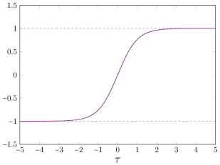
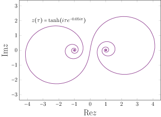
Figure 1: (Left) The instanton solution (3.9) in the imaginary time formalism ($\alpha=\frac{\pi}{2}$), which connects the two potential minima indicated by the horizontal dashed line. (Right) The trajectory of the complex solution obtained by analytic continuation of the instanton solution is shown in the complex plane for $\alpha=0.1\times\frac{\pi}{2}$.

On the other hand, if one plugs (3.11) in the action (3.7), one finds that the $\tau$ integration for different $\alpha$ is related to each other by just rotating the integration contour of $\tau$ in the complex plane, which implies that the action (3.7) is independent of $\alpha$ due to Cauchy’s theorem. Therefore, the transition amplitude one obtains for this solution in the $\alpha\rightarrow 0$ limit is suppressed by $e^{iS[z^{\star}]/\hbar}=e^{-S_{\rm E}/\hbar}$, where $S_{\rm E}>0$ is the Euclidean action for the instanton solution (3.9), which implies that the transition amplitude can be correctly reproduced by the complex saddle point obtained in this way as far as one introduces an infinitesimal $\alpha>0$ as a kind of regulator. In fact, this is confirmed recently including one-loop corrections [14], where the decay rate of a false vacuum has been reproduced correctly based on the optical theorem. However, the singular behaviors in the strict real-time limit $\alpha\rightarrow 0$ still requires clarification. This is important, in particular, since complex trajectories are actually physical objects that can be probed by experiments at least in principle by the so-called weak measurement as we have discussed in subsection 2.4.

4 Monte Carlo results obtained by the GTM

In this section we present our results obtained by Monte Carlo calculations using the GTM. The partition function is given by the transition amplitude (2.23), which is discretized as

$$Z=\int dx\,e^{-S_{\rm eff}(x)}\ ,$$ (4.1)

where $dx=\prod_{n=0}^{N}dx_{n}$ and

$$S_{\rm eff}(x)=-\frac{i\epsilon}{\hbar}\sum_{n=0}^{N-1}\left\{\frac{1}{2}\,m\left(\frac{x_{n+1}-x_{n}}{\epsilon}\right)^{2}-\frac{V(x_{n+1})+V(x_{n})}{2}\right\}-\log\Psi(x_{0})-\log\overline{\Phi(x_{N})}\ .$$ (4.2)

The initial wave function (2.10) is chosen as

$$\Psi(x)=\frac{1}{(2\pi)^{1/4}\sigma^{1/2}}\exp\left\{-\frac{1}{4\sigma^{2}}(x-b)^{2}+\frac{ipx}{\hbar}\right\}\ .$$ (4.3)

If we choose the post-selected wave function as $\Phi(x)=\delta(x-x_{\rm f})$, which amounts to fixing the end point to $x_{N}=x_{\rm f}$, eq. (4.1) reduces to the time-evolved wave function (2.5).

In all the simulations in this work, we set the mass to $m=1$ and the total time to $T=2$, which is divided into $N=20$ intervals. Except in subsection 4.4, where we discuss the semi-classical $\hbar\rightarrow 0$ limit, we set $\hbar=1$. See Appendix A for the details of the method used for our simulations.

4.1 the case of a double-well potential

In this section we consider the case of a double-well potential (3.1) with $a=1$. The height of the potential at the local maximum $x=0$ is $V_{0}=\lambda$. We use $b=-1$ and $\sigma=0.3$ for the initial wave function (4.3) so that it is well localized around $x=-1$, which is one of the potential minima. We use $\Phi(x)=\delta(x-x_{\rm f})$ for the post-selected wave function, where $x_{\rm f}=1$ is chosen to be the other potential minimum.

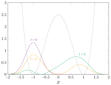
Figure 2: The distribution $|\Psi(x;t)|^{2}$ at time $t=0$ (purple line), $t=2$ (yellow line) and $t=5$ (green line) are shown for the initial wave function (4.3) with $\sigma=0.3$, $b=-1$, $p=0$ in the double-well potential (3.1) with $\lambda=2.5$, $a=1$ (gray, dashed line).

In order to choose an appropriate value for $\lambda$ in the potential to probe quantum tunneling, we consider the probability

$$P=\sum_{E\geq V_{0}}|\langle E|\Psi\rangle|^{2}$$ (4.4)

of the initial quantum state $|\Psi\rangle$ having energy larger than the potential barrier $V_{0}$, where $|E\rangle$ represents the normalized energy eigenstate with the energy $E$. If we choose the momentum $p=0$ in the initial wave function (4.3), we obtain $P\sim 0.11$ for $\lambda=2.5$. We therefore use $\lambda=2.5$ in our calculation.

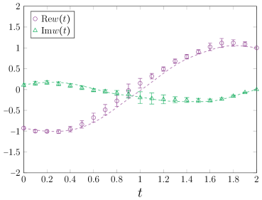
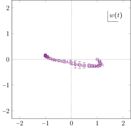
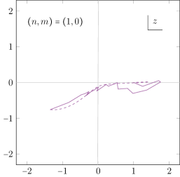
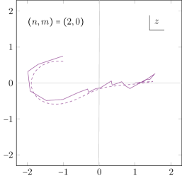
Figure 3: The results obtained for the initial wave function (4.3) with $\sigma=0.3$, $b=-1$, $p=0$ and the post-selected wave function $\Phi(x)=\delta(x-x_{\rm f})$ with $x_{\rm f}=1$ in the double-well potential (3.1) with $\lambda=2.5$, $a=1$. (Top) The weak value of the coordinate is plotted against time $t$ in the Left panel, while the trajectory of the weak value is plotted in the complex plane in the Right panel. The dashed lines represent the result obtained from (2.20) by solving the Schrödinger equation. (Bottom) Two typical trajectories obtained from the numerical simulation with the same parameters as in the Top panels. The dashed lines represent the closest classical solutions obtained by choosing the mode $(n,m)$ and the initial point $x_{\rm i}$ with the final point $x_{\rm f}=1$ fixed.

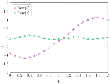
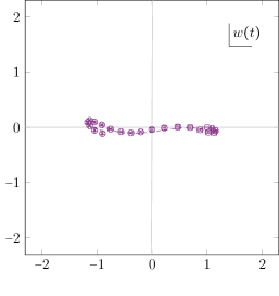
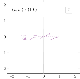
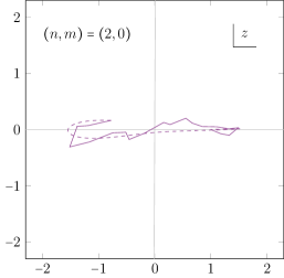
Figure 4: The results obtained for the initial wave function (4.3) with the momentum $p=-2$. All the other parameters are the same as in Fig. 3. (Top) The weak value of the coordinate is plotted against time $t$ in the Left panel, while the trajectory of the weak value is plotted in the complex plane in the Right panel. The dashed lines represent the result obtained from (2.20) by solving the Schrödinger equation. (Bottom) Two typical trajectories obtained from the numerical simulation with the same parameters as in the Top panels. The dashed lines represent the closest classical solutions obtained by choosing the mode $(n,m)$ and the initial point $x_{\rm i}$ with the final point $x_{\rm f}=1$ fixed.

Note that a typical tunneling time can be evaluated by

$$t_{0}\sim\frac{\pi\hbar}{\Delta E}\ ,$$ (4.5)

where $\Delta E$ is the energy difference between the ground state and the first excited state. For $\lambda=2.5$, we find $t_{0}\sim 5$. In Fig. 2 we plot the wave functions at $t=0$, $t=2$ and $t=5$ obtained for this setup by solving the Schrödinger equation with Hamiltonian diagonalization. The result for $t=2$ shows that the significant portion of the distribution has moved to the other potential minimum $x=1$, which implies that quantum tunneling has indeed occurred.

In Fig. 3 (Top), we show our results for the weak value $w(t)$ of the coordinate at time $t$ defined by (2.22) for the initial wave function (4.3) with $\sigma=0.3$, $b=-1$, $p=0$ and the post-selected wave function $\Phi(x)=\delta(x-x_{\rm f})$ with $x_{\rm f}=1$ in the double-well potential (3.1) with $\lambda=2.5$, $a=1$. The dashed lines represent the results obtained directly from (2.20) by solving the Schrödinger equation with Hamiltonian diagonalization. The agreement between our data and the direct results confirms the validity of our calculation. We find that the weak value $w(t)$ is indeed complex except for the end point, which is fixed to $w(T)=x_{\rm f}=1$. Note, in particular, that $w(0)$ is also complex although it is close to $x=-1$, which is the center of the Gaussian wave function (4.3).

In the Bottom panels of Fig. 3, we show two typical trajectories obtained from the simulation with the same parameters as in the Top panels. These trajectories are obtained for a sufficiently long flow time $\tau\sim 4$ in the GTM (See Appendix A.2.) so that they are expected to be close to some relevant saddle points except for fluctuations along the thimble, which are seen as small wiggles in the observed trajectories. Indeed we are able to find a classical solution discussed in section 3.1 which is close to each of these trajectories by choosing the mode $(n,m)$ and the initial point $x_{\rm i}$ with the final point $x_{\rm f}=1$ fixed. We find that the typical trajectories have a larger imaginary part on the left and a smaller imaginary part on the right, which suggests that quantum tunneling occurs first and then some classical motion follows. This feature is obscured in the weak value $w(t)$ shown in the Top-Right panel. This is possible since the weak value $w(t)$ is a weighted average of $x(t)$ obtained from the simulation, where the weight (A.7) is complex in general since it consists of the phase factor $e^{-i\,{\rm Im}S_{\rm eff}}$ and the Jacobian for the change of variables.

Next we introduce nonzero momentum $p=-2$ in the initial wave function (4.3). In Fig. 4 we show our results with all the other parameters the same as in Fig. 3. Since the initial kinetic energy is $p^{2}/2=2$, which is close to the potential barrier $\lambda=2.5$, a classical motion over the potential barrier is possible if the initial point $x(0)$ is slightly shifted from the potential minimum. Indeed we find that the weak value and the typical trajectories become close to real.

4.2 the case with a Gaussian post-selected wave function

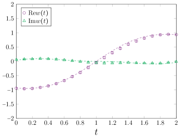
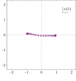
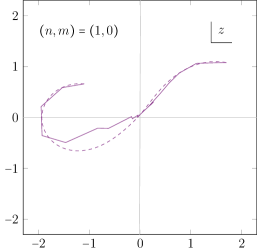
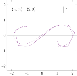
Figure 5: The results obtained for a post-selected wave function (4.6) with all the other parameters the same as in Fig. 3. (Top) The weak value of the coordinate is plotted against time $t$ in the Left panel, while the trajectory of the weak value is plotted in the complex plane in the Right panel. The dashed lines represent the result obtained from (2.20) by solving the Schrödinger equation. (Bottom) Two typical trajectories obtained from the numerical simulation with the same parameters as in the Top panels. The dashed lines represent the closest classical solutions obtained by choosing not only the mode $(n,m)$ and the initial point $x_{\rm i}$ but also the final point $x_{\rm f}$ unlike the previous cases.

So far, we have been fixing the end point to the other potential minimum $x_{\rm f}=1$. This, in particular, allows us to see what kind of trajectories dominate the real-time path integral for the time-evolved wave function (2.1) in the Picard-Lefschetz theory. We were able to see that complex saddle points indeed dominate by choosing the parameters in the initial wave function and the double-well potential appropriately.

On the other hand, the analytic continuation of the instanton solution suggests that the relevant complex trajectory that describes quantum tunneling in the case of a double-well potential has a spiral shape shown in Fig. 1 (Right). In order to clarify the relationship to this result, we consider a post-selected wave function $\Phi(x)$ other than $\Phi(x)=\delta(x-x_{\rm f})$ in the real-time path integral (2.23).

In fact, considering the parity symmetry $x\mapsto-x$ of the quantum system at hand, it is natural to choose the post-selected wave function as

$$\Phi(x)=\Psi(-x)\ ,$$ (4.6)

where the initial wave function $\Psi(x)$ is given by (4.3). This makes the saddle-point equation (2.9) invariant under simultaneous reflection of time $t\mapsto T-t$ and space $z\mapsto-z$, and hence allows a solution with the symmetry $z(T-t)=-z(t)$, which is compatible with the spiral shape in Fig. 1 (Right).

In Fig. 5 we show our results for the initial wave function (4.3) with all the parameters the same as in Fig. 3 and the post-selected wave function now given by (4.6). Unlike the previous cases with $\Phi(x)=\delta(x-x_{\rm f})$, the end point of the trajectories is not constrained to $x(N)=x_{\rm f}$ and it flows into the complex plane due to the flow equation (2.7). In particular, the typical trajectory shown in Fig. 5 (Bottom-Right) has a spiral shape with the symmetry $z(T-t)=-z(t)$, which resembles the trajectory in Fig. 1 (Right) obtained by analytic continuation of the instanton solution. Furthermore the classical solutions that appear in our simulation are all regular even though we are working in the strict real-time limit $\alpha\rightarrow 0$ discussed in section 3.2. It is conceivable that the spiral winds more and more around the potential minima as we increase the time $T$. We also note that the weak value shown in the Top-Right panel turns out to be quite close to real, which is possible since there are more than one relevant complex saddle points that interfere with each other. We consider that the situation is similar to the case with the post-selected quantum state $|\Phi\rangle=\hat{U}(T)\,|\Psi\rangle$ discussed at the end of section 2.4.

4.3 the case of a quartic potential

In this section we discuss the case of a quartic potential

$$V(x)=\kappa\,x^{4}\ ,$$ (4.7)

in which there is no potential barrier to tunnel through.

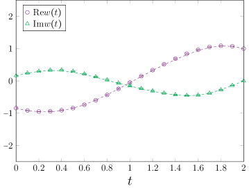
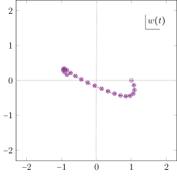
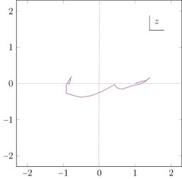
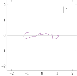
Figure 6: The results obtained for the quartic potential (4.7) with $\kappa=1$. As in Fig. 3, the initial wave function is chosen as (4.3) with $\sigma=0.3$, $b=-1$, $p=0$ and the post-selected wave function is chosen as $\Phi(x)=\delta(x-x_{\rm f})$ with $x_{\rm f}=1$. (Top) The weak value of the coordinate is plotted against time $t$ in the Left panel, while the trajectory of the weak value is plotted in the complex plane in the Right panel. The dashed lines represent the result obtained from (2.20) by solving the Schrödinger equation. (Bottom) Two typical trajectories obtained from the numerical simulation with the same parameters as in the Top panels.

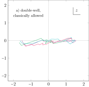
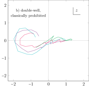
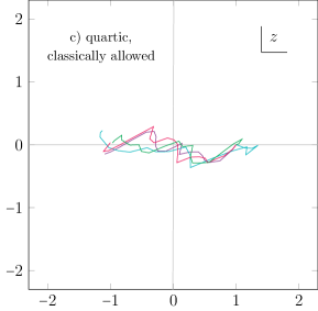
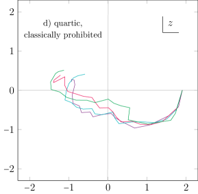
Figure 7: Typical trajectories for $\hbar=0.5$ obtained in various cases. (Top-Left) The case with a double-well potential with all the parameters other than $\hbar$ being the same as in Fig. 3. In particular, the initial wave function is chosen as (4.3) with $b=-1$, $\sigma=0.3$, $p=0$. (Top-Right) The same as the Top-Left panel except that the initial wave function is chosen now as (4.3) with $b=-0.8$, $\sigma=0.2$, $p=0$. (Bottom-Left) The case with a quartic potential with all the parameters other than $\hbar$ being the same as in Fig. 6. In particular, the end point is fixed to $x_{\rm f}=1$. (Bottom-Right) The same as the Bottom-Left panel except that the end point is now fixed to $x_{\rm f}=1.9$.

In Fig. 6 we show our results for $\kappa=1$. As in section 4.1, the initial wave function is chosen as (4.3) with $\sigma=0.3$, $b=-1$, $p=0$ and the post-selected wave function is chosen as $\Phi(x)=\delta(x-x_{\rm f})$ with $x_{\rm f}=1$.

The typical trajectories shown in the Bottom panel are close to real, which suggests that classical motions are allowed with the chosen parameters. Note, however, that, the weak value shown in the Top-Right panel turns out to be complex, which can be understood as a result of interference among various trajectories with relative complex weights. This is in contrast to the situation with the $p=-2$ case discussed in section 4.1, where the typical trajectories and the weak value are both close to real.

4.4 the semi-classical limit

So far, we have chosen $\hbar=1$ in (4.2) and (4.3). In this section, we reduce it to $\hbar=0.5$ and discuss what happens in the semi-classical limit.

Let us consider the double-well potential case with $p=0$ shown in Fig. 3, where typical trajectories are complex for $\hbar=1$. With all the parameters being the same, here we reduce $\hbar$ to $\hbar=0.5$. In Fig. 7 (Top-Left), we find that typical trajectories are close to real suggesting the dominance of real saddle points corresponding to some classical motions. These classical motions are possible since for the initial position $x\leq-\sqrt{2}$, the potential energy (3.1) of the particle becomes larger than the potential barrier $V_{0}=\lambda$. Indeed we find that the initial point $z(0)$ is close to $x=-\sqrt{2}$. Namely, for this setup, we expect that real saddle points dominate in the $\hbar\rightarrow 0$ limit.

Here we change the parameters in the initial wave function (4.3) from the previous ones $b=-1$, $\sigma=0.3$ to the new ones $b=-0.8$, $\sigma=0.2$ with $p=0$ unchanged so that the initial wave function is almost zero at $x\leq-\sqrt{2}$. In Fig. 7 (Top-Right), we indeed find that typical trajectories in this case are complex for $\hbar=0.5$. Namely, for this setup, we expect that complex saddle points dominate in the $\hbar\rightarrow 0$ limit.

Next we consider the quartic potential case shown in Fig. 6, where typical trajectories are close to real for $\hbar=1$. With all the parameters being the same, here we reduce $\hbar$ to $\hbar=0.5$. In Fig. 7 (Bottom-Left), we find that typical trajectories are still close to real suggesting the dominance of real saddle points corresponding to some classical motions. These classical motions are possible since for the initial position $x\leq-1$, the potential energy is larger than the potential energy $V_{0}=\kappa$ at the end point $x_{\rm f}=1$. Namely, for this setup, we expect that real saddle points dominate in the $\hbar\rightarrow 0$ limit.

Here we change the end point from the previous one $x_{\rm f}=1$ to the new one $x_{\rm f}=1.9$ with all the other parameters unchanged. In order to have a classical motion, the initial position should be $x\leq-1.9$, where the initial wave function is almost zero for $b=-1$ and $\sigma=0.3$. In Fig. 7 (Bottom-Right), we indeed find that typical trajectories in this case are complex for $\hbar=0.5$. Namely, for this setup, we expect that complex saddle points dominate in the $\hbar\rightarrow 0$ limit. This case highlights the role played by the post-selection in characterizing quantum tunneling.

5 Summary and discussions

In this paper we have investigated the description of quantum tunneling in the real-time path integral formalism, in which complex trajectories were expected to play a crucial role. In particular, we were able to determine, for the first time, the complex saddle points that are relevant from the viewpoint of the Picard-Lefschetz theory using Monte Carlo methods. The severe sign problem that occurs in evaluating the oscillating integral was overcome by the GTM with various new techniques developed recently. Our results establish a statement that quantum tunneling is characterized by complex saddle points, which dominate the path integral in the semi-classical limit when the classical motion is not allowed by boundary conditions. We have also clarified the relationship to the instanton, which is widely used as a standard description of quantum tunneling based on the imaginary-time path integral formalism.

Among various applications of the description of quantum tunneling in the real-time path integral formalism, we consider that the false vacuum decay is important in the context of cosmology and particle physics [35]. We would also like to recall that quantum tunneling is expected to have taken place at the beginning of our universe [36, 37]. The problem here was that there seemed to be no guiding principle to choose the integration contour in the path integral formalism and hence it was not possible to determine the saddle points that actually contribute [38]. This problem was solved recently by the recognition that quantum gravity should be formulated using the real-time (or Lorentzian) path integral based on the Picard-Lefschetz theory [39]. From this point of view, the quantum tunneling at the beginning of the Universe is described by the emergence of Euclidean geometry as a dominant complex saddle point. Aiming at going beyond the minisuperspace approximation, numerical studies of Lorentzian quantum gravity have recently been started [40, 41, 42]. (See Refs. [43, 44] and references therein for earlier works.) The importance of using the Lorentzian metric has also been realized in nonperturbative formulation of superstring theory [45, 46] based on the IKKT matrix model [47]. Recent Monte Carlo studies suggest the emergence of expanding space-time [48, 49] unlike in the Euclidean version of the model [50]. We consider that the insights gained in this work will be important in pursuing these directions further.

Unlike solving the Schrödinger equation, the path integral formalism can be readily extended to many-body systems and field theories once we overcome the sign problem, for instance, by the GTM as we have demonstrated. It should also be emphasized that, unlike the other promising methods [51, 52, 53, 54], the GTM has a peculiar advantage that it is based on the Picard-Lefschetz theory, which enables us to understand nonperturbative effects in terms of nontrivial saddle points and the associated thimbles that appear in evaluating the oscillating integral. This feature of the GTM was made full use of in our work in the context of quantum tunneling, where the connection to semi-classical descriptions was of particular importance. From this point of view, we hope that the GTM is also useful in elucidating various fundamental problems in quantum theory such as the measurement problem and the quantum-to-classical transition based on the decoherence theory [55], which requires the environment to be included in the simulation.

Acknowledgements

We would like to thank Yuhma Asano and Masafumi Fukuma for valuable discussions. The computations were carried out on the PC clusters in KEK Computing Research Center and KEK Theory Center. K.S. is supported by the Grant-in-Aid for JSPS Research Fellow, No. 20J00079. A. Y. is supported by a Grant-in-Aid for Transformative Research Areas ”The Natural Laws of Extreme Universe—A New Paradigm for Spacetime and Matter from Quantum Information” (KAKENHI Grant No. JP21H05191) from JSPS of Japan.

Appendix A The calculation method used in this work

In this Appendix, we discuss how we obtained the Monte Carlo results presented in section 4. First we briefly review the basic idea of the GTM to solve the sign problem. Then we review the idea of integrating the flow time to solve the multi-modality problem, and discuss how to apply the HMC algorithm, which enables efficient simulation. Finally we explain the problem of the anti-holomorphic gradient flow that occurs in large systems, and discuss how to solve it by optimizing the gradient flow.

A.1 the basic idea of the GTM

In this section we give a brief review of the GTM, which is a promising method for solving the sign problem based on the Picard-Lefschetz theory. Here we consider a general model defined by the partition function and the observable

$$Z=\int d^{N}x\,e^{-S(x)}\ ,\quad\langle\mathcal{O}\rangle=\frac{1}{Z}\int d^{N}x\,\mathcal{O}(x)\,e^{-S(x)}\ ,$$ (A.1)

where $x=(x_{1},x_{1},\cdots,x_{N})\in{\mathbb{R}}^{N}$ and $d^{N}x=\prod_{n=1}^{N}dx_{n}$. The action $S(x)$ is a complex-valued holomorphic function of $x$, which makes (A.1) a highly oscillating multi-dimensional integral and hence causes the sign problem when the number $N$ of variables becomes large. This general partition (A.1) includes the real-time path integral (4.1) with the action (4.2).

Let us first recall that the Picard-Lefschetz theory makes the oscillating integral well-defined by deforming the integration contour using the anti-holomorphic gradient flow equation

$$\frac{dz_{i}(\sigma)}{d\sigma}=\overline{\frac{\partial S(z(\sigma))}{\partial z_{i}}}$$ (A.2)

with the initial condition $z(0)=x\in\mathbb{R}^{N}$, where $\sigma$ plays the role of the deformation parameter. See Eq. (2.7) and below in section 2.2. This flow equation defines a one-to-one map from $x=z(0)\in{\mathbb{R}}^{N}$ to $z=z(\tau)\in\mathcal{M}_{\tau}\in{\mathbb{C}}^{N}$. Due to Cauchy’s theorem, the partition function and the observable (A.1) can be rewritten as

$$Z=\int_{\mathcal{M}_{\tau}}d^{N}z\,e^{-S(z)}\ ,\quad\langle\mathcal{O}\rangle=\frac{1}{Z}\int_{\mathcal{M}_{\tau}}d^{N}z\,\mathcal{O}(z)\,e^{-S(x)}\ .$$ (A.3)

In the $\tau\rightarrow\infty$ limit, ${\rm Im}\,S(z)$ becomes constant on each Lefschetz thimble due to the property (2.8) so that the sign problem is solved except for the one coming from the measure $d^{N}z$. In the GTM [19], the flow time $\tau\rightarrow\infty$ limit is not taken. This has a significant advantage over the earlier proposals [20, 21, 22] with $\tau=\infty$, which require prior knowledge of the relevant saddle points. The sign problem can still be ameliorated by choosing $\tau\sim\log N$, which makes the reweighting method work. However, the large flow time $\tau$ causes the multi-modality problem (or the ergodicity problem) since the transitions among different regions of $\mathcal{M}_{\tau}$ that flow into different thimbles in the $\tau\rightarrow\infty$ limit are highly suppressed during the simulation.

A.2 integrating the flow time

In order to solve both the sign problem and the multi-modality problem, it was proposed [25] to integrate the flow time $\tau$ as

$$Z_{W}=\int_{\tau_{\rm min}}^{\tau_{\rm max}}d\tau\,e^{-W(\tau)}\int_{\mathcal{M}_{\tau}}d^{N}z\,e^{-S(z)}$$ (A.4)

with some weight $W(\tau)$, which is chosen to make the $\tau$-distribution roughly uniform in the region $[\tau_{\rm min},\tau_{\rm max}]$. The use of this idea is important in our work since we have to be able to sample all the saddle points and the associated thimbles that contribute to the path integral. The validity of our simulation in this regard is confirmed by reproducing the correct results for the weak value, which is an ensemble average of the sampled trajectories. See the Top panels in Figs. 3, 4, 5 and 6.

For an efficient sampling in (A.4), we use the Hybrid Monte Carlo algorithm [56], which updates the configuration by solving a fictitious classical Hamilton dynamics treating ${\rm Re}S(z)$ as the potential. When we apply this idea to (A.4), there are actually two options.

One option is to define a fictitious classical Hamilton dynamics for $(z,\tau)\in\mathcal{R}$ with $z\in\mathcal{M}_{\tau}$, where $\mathcal{R}$ is the “worldvolume” obtained by the foliation of $\mathcal{M}_{\tau}$ with $\tau\in[\tau_{\rm min},\tau_{\rm max}]$. While this option has an important advantage (See footnote 14.), one has to treat a system constrained on the worldvolume, which makes the algorithm quite complicated. Another problem is that the worldvolume is pinched if there is a saddle point on the original integration contour, which causes the ergodicity problem.

Here we adopt the other option, which is to rewrite (A.4) as

$$Z_{W}=\int_{\tau_{\rm min}}^{\tau_{\rm max}}d\tau\,e^{-W(\tau)}\int d^{N}x\,\det J(x,\tau)e^{-S(z(x,\tau))}\ ,$$ (A.5)

where $z(x,\tau)$ represents the configuration obtained after the flow starting from $x\in{\mathbb{R}}^{N}$ and

$$J_{ij}(x,\tau)=\frac{\partial z_{i}(x,\tau)}{\partial x_{j}}$$ (A.6)

is the Jacobi matrix associated with the change of variables. Then one can define a fictitious classical Hamilton dynamics for $(x,\tau)\in{\mathbb{R}}^{N}\times[\tau_{\rm min},\tau_{\rm max}]$. Here one only has to deal with an unconstrained system, which makes the algorithm simple. The disadvantage, however, is that the Jacobian $\det J(x,\tau)$ that appears in (A.5) has to be taken into account by reweighting, which causes the overlap problem when the modulus $|\det J(x,\tau)|$ fluctuates considerably during the simulation. In that case, only a small number of configurations with large $|\det J(x,\tau)|$ dominate the ensemble average and hence the statistics cannot be increased efficiently. It turns out that this problem does not occur in the simulations performed in this work if we optimize the flow equation as we describe in section A.4. In all the simulations, we have chosen $\tau_{\rm min}=0.2$, which is small enough to solve the multi-modality problem, and $\tau_{\rm max}=4$, which is large enough to obtain typical trajectories close to the relevant saddle points. Note also that the sign problem is solved already at $\tau\sim 2$.

Once we generate the configurations $(x,\tau)$, we can calculate the expectation value $\langle\mathcal{O}\rangle$ by taking the ensemble average of $\mathcal{O}(z(x,\tau))$ with the reweighting factor

$$R(x,\tau)=\det J(x,\tau)\,e^{-i\,{\rm Im}S(z(x,\tau))}$$ (A.7)

using the configurations $(x,\tau)$ obtained for an appropriate range of $\tau$ [57].

In either option of the HMC algorithm, the most time-consuming part is the calculation of the Jacobian $\det J(x,\tau)$, which requires O($N^{3}$) computational cost in the reweighting procedure. In order to calculate the Jacobi matrix $J(x,\tau)$, one has to solve the flow equation

$$\frac{\partial}{\partial\sigma}J_{ij}(\sigma)=\overline{H_{ik}(z(\sigma))\,J_{kj}(\sigma)}$$ (A.8)

with the initial condition $J(0)=\textbf{1}_{N}$, where we have defined the Hessian

$$H_{ij}(z) =\frac{\partial^{2}S(z)}{\partial z_{i}\partial z_{j}}\ .$$ (A.9)

A.3 backpropagating Hybrid Monte Carlo algorithm

In this section we review the backpropagating HMC algorithm [24], which is crucial in simulating the system (A.5). Here we discuss the case of fixed flow time $\tau$ for simplicity and comment on the case of integrating $\tau$ at the end of this section.

The first step of the HMC algorithm [56] is to introduce new variables $p_{i}$ ($i=1,\cdots,N$) with the partition function

$$Z_{\text{HMC}}=\int d^{N}x\,d^{N}p\,e^{-\frac{p^{2}}{2}-\text{Re}S(z(x,\tau))}\ ,$$ (A.10)

where the Gaussian integral of $p$ simply yields a constant factor. In order to update the configuration $(x,p)$, we first generate $p$ with the probability distribution $\propto\exp(-p^{2}/2)$ and solve the fictitious Hamilton equation with the Hamiltonian

$$H(x,p)=\frac{1}{2}\sum_{i=1}^{N}p_{i}^{2}+\text{Re}S(z(x,\tau))\ ,$$ (A.11)

which reads

$$\frac{dx_{i}(s)}{ds} =p_{i}(s)\ ,$$ (A.12)

$$\frac{dp_{i}(s)}{ds} =F_{i}(s)$$ (A.13)

with the force $F_{i}(s)$ defined by

$$F_{i}(s) =-\left.\frac{\partial{\rm Re}S(z(x,\tau))}{\partial x_{i}}\right|_{x=x(s)}\ .$$ (A.14)

We solve the Hamilton equation (A.12) and (A.13) for a fixed time $s_{\rm f}$ to obtain a new configuration $x(s_{\rm f})$ and $p(s_{\rm f})$.

In actual calculation, we discretize the Hamilton equation using the standard leap-frog discretization, which respects the reversibility and the preservation of the phase space volume [56]. Let us divide the total time $s_{\rm f}$ into $N_{\rm s}$ segments as $s_{\rm f}=N_{\rm s}\Delta s$. Then we define the discretized Hamilton equation as

$$x_{i}(s_{n+1/2}) =x_{i}(s_{n})+\frac{\Delta s}{2}\,p_{i}(s_{n})\ ,$$ (A.15)

$$p_{i}(s_{n+1}) =p_{i}(s_{n})+\Delta s\,F_{i}(s_{n+1/2})\ ,$$ (A.16)

$$x_{i}(s_{n+1}) =x_{i}(s_{n+1/2})+\frac{\Delta s}{2}\,p_{i}(s_{n+1})$$ (A.17)

for $n=0,1,...,N_{s}-1$, where $s_{\nu}=\nu\Delta s$ with $\nu$ being an integer or a half integer. Since the Hamiltonian conservation is violated by the discretization, we have to treat the new configuration given by $x(s_{\rm f})$ and $p(s_{\rm f})$ as a trial configuration, which is subject to the Metropolis accept/reject procedure with the acceptance probability $\min(1,e^{-\delta H})$, where

$$\delta H =H(x(s_{\rm f}),p(s_{\rm f}))-H(x(0),p(0))\ ,$$ (A.18)

which guarantees the detail balance exactly. The parameters $s_{\rm f}$ and $N_{\rm s}$ in the HMC algorithm can be optimized in a standard way by minimizing the computational cost required for generating a statistically independent configuration.

Note that the force (A.14) can be rewritten as

$$F_{i}(s)=f_{j}(s)J_{ji}(x(s),\tau)+\overline{f_{j}(s)J_{ji}(x(s),\tau)}\ ,$$ (A.19)

where we define the “force”

$$f_{i}(s) =-\left.\frac{\partial{\rm Re}S(z)}{\partial z_{i}}\right|_{z=z(x(s),\tau)}$$ (A.20)

at $z(x(s),\tau)$ on the deformed contour $\mathcal{M}_{\tau}$. If we use eq. (A.19) to calculate the force, we need to calculate the Jacobi matrix $J_{ji}(x(s),\tau)$ at each step of solving the Hamilton equation. It was found recently [24] that this can be avoided by using backpropagation as we explain below.

Let us first rewrite the flow equations for the configuration (A.2) and the Jacobi matrix (A.8) in the discretized form as

$$z_{i}(\sigma+\epsilon) =z_{i}(\sigma)+\epsilon\,\overline{\frac{\partial S(z(\sigma))}{\partial z_{i}}}\ ,$$ (A.21)

$$J_{ij}(\sigma+\epsilon) =J_{ij}(\sigma)+\epsilon\,\overline{H_{ik}(z(\sigma))J_{kj}(\sigma)}\ .$$ (A.22)

Note that (A.22) can be written in a matrix notation as

$$\left(\begin{matrix}J(\sigma+\epsilon)\\ \overline{J(\sigma+\epsilon)}\end{matrix}\right) =\mathcal{U}(\sigma)\left(\begin{matrix}J(\sigma)\\ \overline{J(\sigma)}\end{matrix}\right)\ ,$$ (A.23)

$$\mathcal{U}(\sigma) =\left(\begin{matrix}\textbf{1}_{N}&\epsilon\overline{H(z(\sigma))}\\ \epsilon H(z(\sigma))&\textbf{1}_{N}\end{matrix}\right)\ .$$ (A.24)

Using this, we can rewrite the force (A.19) as

$$F^{\top}(s) =\left(\begin{matrix}f^{\top}(s)&\bar{f}\,{}^{\top}(s)\end{matrix}\right)\left(\begin{matrix}J(\tau)\\ \overline{J(\tau)}\end{matrix}\right)$$

$$=\left(\begin{matrix}f^{\top}(s)&\bar{f}\,{}^{\top}(s)\end{matrix}\right)\mathcal{U}(\tau-\epsilon)\,\mathcal{U}(\tau-2\epsilon)\cdots\mathcal{U}(2\epsilon)\,\mathcal{U}(\epsilon)\left(\begin{matrix}\textbf{1}_{N}\\ \textbf{1}_{N}\end{matrix}\right)\ .$$ (A.25)

Note that evaluating this quantity by multiplying the matrices from the right corresponds to using eq. (A.19) naively to calculate the force. This requires matrix-matrix multiplications, which cost O($N^{3}$) computation time or O($N^{2}$) if the Hessian is sparse as in local systems. However, we can actually evaluate (A.25) by multiplying the matrices from the left, which corresponds to backpropagating the force on the deformed contour to the original contour. This requires only vector-matrix multiplications and thus reduces the computational cost by the order of O($N$) in this procedure.

In our simulation, we actually use the optimized flow equation explained in the next section, and hence the flow equations (A.21) and (A.22) have to be modified accordingly. However, the idea of backpropagation remains applicable.

So far we have explained the idea of the HMC algorithm for a fixed flow time $\tau$ for simplicity. In actual simulation, however, we also integrate the flow time $\tau$ as in (A.5) to avoid the multi-modality problem. Accordingly, we have to treat $\tau$ as a dynamical variable in the HMC algorithm together with its conjugate momentum $p_{\tau}$. The partition function (A.10) should then be replaced by

$$\tilde{Z}_{\rm HMC} =\int d\tau\,dp_{\tau}\,dx\,dp\,e^{-H}\ ,$$ (A.26)

$$H =\frac{1}{2m(\tau)}(p_{i})^{2}+\frac{1}{2}(p_{\tau})^{2}+{\rm Re}S(z(x,\tau))+W(\tau)\ ,$$ (A.27)

where we introduce the $\tau$-dependent mass function $m(\tau)$. See section 6.1 of Ref. [24] for the details. Here we just mention that $m(\tau)$ should be chosen to be proportional to the typical value of $|\det J(x,\tau)|^{2/N}$ for various $x$ with fixed $\tau$ so that the simulation can realize a random walk on the deformed manifold with almost uniform discretization. Also the weight function $W(\tau)$ in (A.5) should be chosen so that the distribution of $\tau$ obtained by simulations becomes as uniform as possible within the region $\tau_{\rm min}\leq\tau\leq\tau_{\rm max}$. The functions $m(\tau)$ and $W(\tau)$ used in each simulation are parametrized as

$$m(\tau) =m_{0}+m_{1}\tau\ ,$$ (A.28)

$$W(\tau) =\sum_{k=1}^{6}w_{k}\tau^{k}\ .$$ (A.29)

We use $m_{0}=-0.209$ and $m_{1}=1.5851$ for all cases, while $w_{k}$ are chosen as in Table 1.

Figure	$w_{1}$	$w_{2}$	$w_{3}$	$w_{4}$	$w_{5}$	$w_{6}$
Fig.3	-26.4297	25.8099	-13.814	4.0988	-0.6254	0.0382
Fig.4	-31.949	35.409	-21.3925	7.0716	-1.1934	0.0805
Fig.5	-33.9717	36.9599	-21.7341	7.0366	-1.1676	0.0775
Fig.6	-26.344	27.6191	-15.0622	4.5638	-0.7146	0.0452
Fig.7(TL)	-26.4127	25.5518	-13.7184	4.0885	-0.6254	0.0382
Fig.7(TR)	-26.4127	25.5518	-13.7184	4.0885	-0.6254	0.0382
Fig.7(BL)	-27.748	30.1805	-18.2515	6.04706	-1.0202	0.06868
Fig.7(BR)	-64.38	68.644	-40.113	12.9891	-2.1781	0.14779

Table 1: The parameters (A.29) in the function $W(\tau)$ chosen for the case shown in each figure. TL, TR, BL and BR in the left-most column imply Top-Left, Top-Right, Bottom-Left and Bottom-Right, respectively.

As for the parameters in the HMC algorithm, we always use $s_{\rm f}=1$, whereas $N_{\rm s}$ is chosen to be $10$ except for the cases in Fig. 7, where we use $N_{\rm s}=30$ to keep the acceptance rate high enough.

A.4 optimizing the flow equation

In this section, we discuss a problem that occurs when we use the original flow equation (A.2) for a system with many variables such as (4.1) with $N=20$ studied in this paper. We solve this problem by optimizing the flow equation, which actually has large freedom of choice if we are just to satisfy the property (2.8). Here we explain the basic idea and defer a detailed discussion to the forth-coming paper [28].

The problem with the original flow (A.2) can be readily seen by considering how its solution $z(x,\sigma)$ changes when the initial value $z(x,0)=x\in{\mathbb{R}}^{N}$ changes infinitesimally. Note that the displacement $\zeta_{i}(\sigma)\equiv z_{i}(x+\delta x,\sigma)-z_{i}(x,\sigma)$ for an infinitesimal $\delta x$ can be obtained as

$$\zeta_{i}(\sigma)=J_{ij}(\sigma)\,\delta x_{j}\ ,$$ (A.30)

where $J_{ij}(\sigma)$ is the Jacobi matrix at the flow time $\sigma$, which satisfies the flow equation (A.8). Thus we find that the displacement satisfies the flow equation

$$\frac{d\zeta_{i}(\sigma)}{d\sigma}=\overline{H_{ij}(z(\sigma))\,\zeta_{j}(\sigma)}$$ (A.31)

with the boundary condition $\zeta_{i}(0)=\delta x_{i}$, where $H_{ij}(z)$ is the Hessian defined by (A.9).

Let us consider the singular value decomposition (SVD) of the Hessian $H_{ij}(z(\sigma))$ given as

$$H(z(\sigma))=U^{\top}(\sigma)\,\Lambda(\sigma)\,U(\sigma)\ ,$$ (A.32)

where $U(\sigma)$ is a unitary matrix and $\Lambda={\rm diag}(\lambda_{1},\cdots,\lambda_{N})$ is a diagonal matrix with $\lambda_{1}\geq\cdots\geq\lambda_{N}\geq 0$. Plugging this in (A.8), we obtain

$$\frac{dJ(\sigma)}{d\sigma}=U(\sigma)^{\dagger}\,\Lambda(\sigma)\,\overline{U(\sigma)\,J(\sigma)}\ ,$$ (A.33)

and similarly for the displacement

$$\frac{d\zeta(\sigma)}{d\sigma}=U(\sigma)^{\dagger}\,\Lambda(\sigma)\,\overline{U(\sigma)\,\zeta(\sigma)}\ .$$ (A.34)

Roughly speaking, the magnitude of the displacement $\zeta(\sigma)$ grows exponentially with $\sigma$, and the growth rate is given by a weighted average of the singular values with a weight depending on $\delta x$. If the singular values have a hierarchy $\lambda_{1}\gg\lambda_{N}$, some modes grow much faster than the others. This causes a serious technical problem in solving the flow equation since it may easily diverge during the procedure.

In order to solve this problem, we pay attention to the freedom in defining the flow equation. As we discussed in section 2.2, the important property of the flow equation (A.2) is (2.8). Let us therefore consider a generalized flow equation

$$\frac{dz_{i}(\sigma)}{d\sigma}=\mathcal{A}_{ij}(z(\sigma),\overline{z(\sigma)})\overline{\frac{\partial S(z(\sigma))}{\partial z_{j}}}\ ,$$ (A.35)

which generalizes the equation (2.8) as

$$\frac{dS(z(\sigma))}{d\sigma}=\sum_{i}\frac{\partial S(z(\sigma))}{\partial z_{i}}\frac{dz_{i}(\sigma)}{d\sigma}=\sum_{ij}\frac{\partial S(z(\sigma))}{\partial z_{i}}\mathcal{A}_{ij}(z(\sigma),\overline{z(\sigma)})\overline{\frac{\partial S(z(\sigma))}{\partial z_{j}}}\ .$$ (A.36)

For this to be positive semi-definite, the kernel $\mathcal{A}_{ij}(z,\bar{z})$ has only to be Hermitian positive, and it does not have to be holomorphic.

Accordingly, the flow of the Jacobi matrix becomes

$$\frac{\partial}{\partial\sigma}J_{ij}(\sigma)=\mathcal{A}_{ik}\overline{H_{kl}(z(\sigma))\,J_{lj}(\sigma)}+\left(\frac{\partial\mathcal{A}_{il}}{\partial z_{k}}J_{kj}(\sigma)+\frac{\partial\mathcal{A}_{il}}{\partial\bar{z}_{k}}\overline{J_{kj}(\sigma)}\right)\overline{\frac{\partial S(z(\sigma))}{\partial z_{l}}}\ .$$ (A.37)

Note that the discretized version of (A.37) can still be written in the form (A.23), which means that the backpropagation [24] can be used even with the generalized flow equation.

From (A.37), we obtain the flow of the displacement as

$$\frac{\partial}{\partial\sigma}\zeta_{i}(\sigma)=\mathcal{A}_{ik}\overline{H_{kl}(z(\sigma))\,\zeta_{l}(\sigma)}+\left(\frac{\partial\mathcal{A}_{il}}{\partial z_{k}}\zeta_{k}(\sigma)+\frac{\partial\mathcal{A}_{il}}{\partial\bar{z}_{k}}\overline{\zeta_{k}(\sigma)}\right)\overline{\frac{\partial S(z(\sigma))}{\partial z_{l}}}\ .$$ (A.38)

Let us here assume that the first term is dominant in (A.38). Then plugging (A.32) in (A.38), we obtain

$$\frac{d\zeta(\sigma)}{d\sigma}\sim\mathcal{A}\,U(\sigma)^{\dagger}\,\Lambda(\sigma)\,\overline{U(\sigma)\,\zeta(\sigma)}\ .$$ (A.39)

Therefore, by choosing

$$\mathcal{A}=U(\sigma)^{\dagger}\,\Lambda^{-1}(\sigma)\,U(\sigma)\ ,$$ (A.40)

we obtain

$$\frac{d\zeta(\sigma)}{d\sigma}\sim U(\sigma)^{\dagger}\,\overline{U(\sigma)\,\zeta(\sigma)}\ ,$$ (A.41)

in which the problematic hierarchy of singular values $\lambda_{i}$ in (A.34) is completely eliminated. From this point of view, (A.40) seems to be the optimal choice for the “preconditioner” $\mathcal{A}$ in the generalized flow equation (A.35). Note also that, under a similar assumption, the flow of the Jacobi matrix changes from (A.33) to

$$\frac{\partial}{\partial\sigma}J(\sigma)\sim U(\sigma)^{\dagger}\,\overline{U(\sigma)\,J(\sigma)}\ .$$ (A.42)

Thus, in our simulation, the use of the optimal flow equation solves the overlap problem that actually occurs otherwise due to the large fluctuation of $|\det J|$. (See the discussions below (A.6).)

In order to implement this idea, let us first note that (A.40) can be written as

$$\mathcal{A}(z(\sigma),\overline{z(\sigma)}) =\Big{\{}H^{\dagger}(z(\sigma))H(z(\sigma))\Big{\}}^{-1/2}=\Big{\{}\overline{H(z(\sigma))}H(z(\sigma))\Big{\}}^{-1/2}\ .$$ (A.43)

Here we use the rational approximation

$$x^{-1/2} \approx a_{0}+\sum_{q=1}^{Q}\frac{a_{q}}{x+b_{q}}\ ,$$ (A.44)

which can be made accurate for a wide range of $x$ with the real positive parameters $a_{q}$ and $b_{q}$ generated by the Remez algorithm. Thus we obtain

$$\mathcal{A}(z,\bar{z}) \approx a_{0}\,\textbf{1}_{N}+\sum_{q=1}^{Q}a_{q}\,\Big{\{}\overline{H(z)}H(z)+b_{q}\,\textbf{1}_{N}\Big{\}}^{-1}\ .$$ (A.45)

With this expression, the derivative of $\mathcal{A}$ in (A.37) can be calculated straightforwardly as

$$\frac{\partial\mathcal{A}}{\partial z_{k}} =-\sum_{q=1}^{Q}a_{q}(\bar{H}H+b_{q}\textbf{1}_{N})^{-1}\bar{H}\frac{\partial H}{\partial z_{k}}(\bar{H}H+b_{q}\textbf{1}_{N})^{-1}\ ,$$ (A.46)

$$\frac{\partial\mathcal{A}}{\partial\bar{z}_{k}} =-\sum_{q=1}^{Q}a_{q}(\bar{H}H+b_{q}\textbf{1}_{N})^{-1}\overline{\frac{\partial H}{\partial z_{k}}}H(\bar{H}H+b_{q}\textbf{1}_{N})^{-1}\ .$$ (A.47)

The matrix inverse $(\bar{H}H+b_{q}\textbf{1}_{N})^{-1}$ does not have to be calculated explicitly since it only appears in the algorithm as a matrix that acts on a particular vector, which allows us to use an iterative method for solving a linear equation such as the conjugate gradient (CG) method. The factor of $Q$ in the computational cost can be avoided by the use of a multi-mass CG solver [59]. These techniques are well known in the so-called Rational HMC algorithm [60, 61], which is widely used in QCD with dynamical strange quarks [62] and supersymmetric theories such as the BFSS and IKKT matrix models (See Refs. [63, 64, 45], for example.).

References

- [1] S. Coleman, Aspects of Symmetry: Selected Erice Lectures, Cambridge University Press (1985), 10.1017/CBO9780511565045.
- [2] S. Coleman, Fate of the false vacuum: Semiclassical theory, Phys. Rev. D 15 (1977) 2929.
- [3] C.G. Callan and S. Coleman, Fate of the false vacuum. ii. first quantum corrections, Phys. Rev. D 16 (1977) 1762.
- [4] S. Abel and M. Spannowsky, Observing the fate of the false vacuum with a quantum laboratory, PRX Quantum 2 (2021) 010349 [2006.06003].
- [5] T. Markkanen, A. Rajantie and S. Stopyra, Cosmological Aspects of Higgs Vacuum Metastability, Front. Astron. Space Sci. 5 (2018) 40 [1809.06923].
- [6] M. Stone, The Lifetime and Decay of Excited Vacuum States of a Field Theory Associated with Nonabsolute Minima of Its Effective Potential, Phys. Rev. D 14 (1976) 3568.
- [7] P.H. Frampton, Vacuum Instability and Higgs Scalar Mass, Phys. Rev. Lett. 37 (1976) 1378.
- [8] M. Stone, Semiclassical Methods for Unstable States, Phys. Lett. B 67 (1977) 186.
- [9] P.H. Frampton, Consequences of Vacuum Instability in Quantum Field Theory, Phys. Rev. D 15 (1977) 2922.
- [10] T. Onishi, A. Shudo, K.S. Ikeda and K. Takahashi, Semiclassical study on tunneling processes via complex-domain chaos, Phys. Rev. E 68 (2003) 056211.
- [11] N. Turok, On Quantum Tunneling in Real Time, New J. Phys. 16 (2014) 063006 [1312.1772].
- [12] Y. Tanizaki and T. Koike, Real-time Feynman path integral with Picard–Lefschetz theory and its applications to quantum tunneling, Annals Phys. 351 (2014) 250 [1406.2386].
- [13] A. Cherman and M. Unsal, Real-Time Feynman Path Integral Realization of Instantons, 1408.0012.
- [14] W.-Y. Ai, B. Garbrecht and C. Tamarit, Functional methods for false vacuum decay in real time, JHEP 12 (2019) 095 [1905.04236].
- [15] Z.-G. Mou, P.M. Saffin, A. Tranberg and S. Woodward, Real-time quantum dynamics, path integrals and the method of thimbles, JHEP 06 (2019) 094 [1902.09147].
- [16] Z.-G. Mou, P.M. Saffin and A. Tranberg, Quantum tunnelling, real-time dynamics and Picard-Lefschetz thimbles, JHEP 11 (2019) 135 [1909.02488].
- [17] J. Braden, M.C. Johnson, H.V. Peiris, A. Pontzen and S. Weinfurtner, New Semiclassical Picture of Vacuum Decay, Phys. Rev. Lett. 123 (2019) 031601 [1806.06069].
- [18] M.P. Hertzberg and M. Yamada, Vacuum Decay in Real Time and Imaginary Time Formalisms, Phys. Rev. D 100 (2019) 016011 [1904.08565].
- [19] A. Alexandru, G. Basar, P.F. Bedaque, G.W. Ridgway and N.C. Warrington, Sign problem and monte carlo calculations beyond lefschetz thimbles, JHEP 05 (2016) 053 [1512.08764].
- [20] H. Fujii, D. Honda, M. Kato, Y. Kikukawa, S. Komatsu and T. Sano, Hybrid monte carlo on lefschetz thimbles - a study of the residual sign problem, JHEP 10 (2013) 147 [1309.4371].
- [21] AuroraScience collaboration, New approach to the sign problem in quantum field theories: High density qcd on a lefschetz thimble, Phys.Rev.D 86 (2012) 074506 [1205.3996].
- [22] E. Witten, Analytic continuation of Chern-Simons theory, AMS/IP Stud. Adv. Math. 50 (2011) 347 [1001.2933].
- [23] M. Fukuma, N. Matsumoto and N. Umeda, Implementation of the HMC algorithm on the tempered Lefschetz thimble method, 1912.13303.
- [24] G. Fujisawa, J. Nishimura, K. Sakai and A. Yosprakob, Backpropagating Hybrid Monte Carlo algorithm for fast Lefschetz thimble calculations, JHEP 04 (2022) 179 [2112.10519].
- [25] M. Fukuma and N. Matsumoto, Worldvolume approach to the tempered Lefschetz thimble method, PTEP 2021 (2021) 023B08 [2012.08468].
- [26] M. Fukuma and N. Umeda, Parallel tempering algorithm for integration over lefschetz thimbles, PTEP 2017 (2017) 073B01 [1703.00861].
- [27] A. Alexandru, G. Basar, P.F. Bedaque and N.C. Warrington, Tempered transitions between thimbles, Phys. Rev. D 96 (2017) 034513 [1703.02414].
- [28] J. Nishimura, K. Sakai and A. Yosprakob, in preparation .
- [29] A. Alexandru, G. Basar, P.F. Bedaque, S. Vartak and N.C. Warrington, Monte Carlo Study of Real Time Dynamics on the Lattice, Phys. Rev. Lett. 117 (2016) 081602 [1605.08040].
- [30] A. Alexandru, G. Basar, P.F. Bedaque and G.W. Ridgway, Schwinger-Keldysh formalism on the lattice: A faster algorithm and its application to field theory, Phys. Rev. D 95 (2017) 114501 [1704.06404].
- [31] Y. Aharonov, D.Z. Albert and L. Vaidman, How the result of a measurement of a component of the spin of a spin-1/2 particle can turn out to be 100, Phys. Rev. Lett. 60 (1988) 1351.
- [32] A. Tanaka, Semiclassical theory of weak values, Phys. Lett. A 297 (2002) 307 [quant-ph/0203149].
- [33] E. Picard and G. Simart, Theorie des fonctions algebriques de deux variables independantes. Tome I, (1897) .
- [34] S. Lefschetz, L’analysis situs et la geometrie algebrique, (1924) .
- [35] T. Hayashi, K. Kamada, N. Oshita and J. Yokoyama, Vacuum decay in the Lorentzian path integral, JCAP 05 (2022) 041 [2112.09284].
- [36] A. Vilenkin, Creation of Universes from Nothing, Phys. Lett. B 117 (1982) 25.
- [37] J.B. Hartle and S.W. Hawking, Wave Function of the Universe, Phys. Rev. D 28 (1983) 2960.
- [38] J.J. Halliwell and J. Louko, Steepest Descent Contours in the Path Integral Approach to Quantum Cosmology. 1. The De Sitter Minisuperspace Model, Phys. Rev. D 39 (1989) 2206.
- [39] J. Feldbrugge, J.-L. Lehners and N. Turok, Lorentzian Quantum Cosmology, Phys. Rev. D 95 (2017) 103508 [1703.02076].
- [40] D. Jia, Complex, Lorentzian, and Euclidean simplicial quantum gravity: numerical methods and physical prospects, 2110.05953.
- [41] Y. Ito, D. Kadoh and Y. Sato, Tensor network approach to 2D Lorentzian quantum Regge calculus, Phys. Rev. D 106 (2022) 106004 [2208.01571].
- [42] D. Jia, Truly Lorentzian quantum cosmology, 2211.00517.
- [43] J. Ambjorn, A. Goerlich, J. Jurkiewicz and R. Loll, Nonperturbative Quantum Gravity, Phys. Rept. 519 (2012) 127 [1203.3591].
- [44] R. Loll, Quantum Gravity from Causal Dynamical Triangulations: A Review, Class. Quant. Grav. 37 (2020) 013002 [1905.08669].
- [45] S.-W. Kim, J. Nishimura and A. Tsuchiya, Expanding (3+1)-dimensional universe from a Lorentzian matrix model for superstring theory in (9+1)-dimensions, Phys. Rev. Lett. 108 (2012) 011601 [1108.1540].
- [46] J. Nishimura and A. Tsuchiya, Complex Langevin analysis of the space-time structure in the Lorentzian type IIB matrix model, JHEP 06 (2019) 077 [1904.05919].
- [47] N. Ishibashi, H. Kawai, Y. Kitazawa and A. Tsuchiya, A Large N reduced model as superstring, Nucl. Phys. B 498 (1997) 467 [hep-th/9612115].
- [48] J. Nishimura, Signature change of the emergent space-time in the IKKT matrix model, PoS CORFU2021 (2022) 255 [2205.04726].
- [49] K.N. Anagnostopoulos, T. Azuma, K. Hatakeyama, M. Hirasawa, Y. Ito, J. Nishimura et al., Progress in the numerical studies of the type IIB matrix model, Eur. Phys. J. Spec. Top. (2023) [2210.17537].
- [50] K.N. Anagnostopoulos, T. Azuma, Y. Ito, J. Nishimura, T. Okubo and S. Kovalkov Papadoudis, Complex Langevin analysis of the spontaneous breaking of 10D rotational symmetry in the Euclidean IKKT matrix model, JHEP 06 (2020) 069 [2002.07410].
- [51] J. Berges and I.O. Stamatescu, Simulating nonequilibrium quantum fields with stochastic quantization techniques, Phys. Rev. Lett. 95 (2005) 202003 [hep-lat/0508030].
- [52] J. Berges, S. Borsanyi, D. Sexty and I.O. Stamatescu, Lattice simulations of real-time quantum fields, Phys. Rev. D 75 (2007) 045007 [hep-lat/0609058].
- [53] S. Takeda, Tensor network approach to real-time path integral, PoS LATTICE2019 (2019) 033 [1908.00126].
- [54] S. Takeda, A novel method to evaluate real-time path integral for scalar theory, PoS LATTICE2021 (2022) 532 [2108.10017].
- [55] M. Schlosshauer, Quantum Decoherence, Phys. Rept. 831 (2019) 1 [1911.06282].
- [56] S. Duane, A.D. Kennedy, B.J. Pendleton and D. Roweth, Hybrid Monte Carlo, Phys. Lett. B 195 (1987) 216.
- [57] M. Fukuma, N. Matsumoto and Y. Namekawa, Statistical analysis method for the worldvolume hybrid Monte Carlo algorithm, PTEP 2021 (2021) 123B02 [2107.06858].
- [58] J. Feldbrugge and N. Turok, Existence of real time quantum path integrals, Annals Phys. 454 (2023) 169315 [2207.12798].
- [59] B. Jegerlehner, Krylov space solvers for shifted linear systems, hep-lat/9612014.
- [60] A.D. Kennedy, I. Horvath and S. Sint, A New exact method for dynamical fermion computations with nonlocal actions, Nucl. Phys. B Proc. Suppl. 73 (1999) 834 [hep-lat/9809092].
- [61] M.A. Clark, The Rational Hybrid Monte Carlo Algorithm, PoS LAT2006 (2006) 004 [hep-lat/0610048].
- [62] M.A. Clark, A.D. Kennedy and Z. Sroczynski, Exact 2+1 flavour RHMC simulations, Nucl. Phys. B Proc. Suppl. 140 (2005) 835 [hep-lat/0409133].
- [63] S. Catterall and T. Wiseman, Towards lattice simulation of the gauge theory duals to black holes and hot strings, JHEP 12 (2007) 104 [0706.3518].
- [64] K.N. Anagnostopoulos, M. Hanada, J. Nishimura and S. Takeuchi, Monte Carlo studies of supersymmetric matrix quantum mechanics with sixteen supercharges at finite temperature, Phys. Rev. Lett. 100 (2008) 021601 [0707.4454].