Time-optimal multi-qubit gates: Complexity, efficient heuristic and gate-time bounds

Abstract

Multi-qubit interactions are omnipresent in quantum computing hardware, and they can generate multi-qubit entangling gates. Such gates promise advantages over traditional two-qubit gates. In this work, we focus on the quantum gate synthesis with multi-qubit Ising-type interactions and single-qubit gates. These interactions can generate global $ZZ$-gates ($\operatorname{\mathsf{GZZ}}$ gates). We show that the synthesis of time-optimal multi-qubit gates is $\mathsf{NP}$-hard. However, under certain assumptions we provide explicit constructions of time-optimal multi-qubit gates allowing for efficient synthesis. These constructed multi-qubit gates have a constant gate time and can be implemented with linear single-qubit gate layers. Moreover, a heuristic algorithm with polynomial runtime for synthesizing fast multi-qubit gates is provided. Finally, we prove lower and upper bounds on the optimal $\operatorname{\mathsf{GZZ}}$ gate-time. Furthermore, we conjecture that any $\operatorname{\mathsf{GZZ}}$ gate can be executed in a time $\operatorname{\mathrm{O}}(n)$ for $n$ qubits. We support this claim with theoretical and numerical results.

I Introduction

Any quantum computation requires to decompose its logical operations into the platform’s native instruction set. The performance of the computation depends heavily on the available instructions and their implementation in the quantum hardware. In the era of noisy and intermediate scale quantum (NISQ) devices, a major obstacle is the short decoherence time which limits the runtime of a quantum computation significantly [1]. Therefore, it is not only necessary to optimize the number of native instructions but also their execution time.

Ising-type interactions generate an important and rich class of Hamiltonians which are ubiquitous in quantum computing platforms [2, 3, 4, 5, 6]. Previously, we have utilized these Ising-type interactions in a new synthesis method [7]. In particular, we have considered the problem of synthesizing time-optimal multi-qubit gates on a quantum computing platform that supports the following basic operations:

1. single-qubit rotations can be executed in parallel, and

2. it offers fixed Ising-type interactions.

In Ref. [7], it is shown that this synthesis problem is always solvable, and that a solution minimizing the overall gate time can be found using a linear program. The feasibility of the approach is demonstrated numerically, showing that, in practice, the gate time scales linearly with the number of qubits. However, a systematic analysis has been left for future work.

This work is dedicated to an in-depth study of the time-optimal synthesis problem. We draw the connection between the synthesis of time-optimal multi-qubit gates and graph theory. The cut polytope is defined as the convex hull of binary vectors representing the possible cuts of a given graph [8]. We provide a polynomial time reduction of the membership problem of the cut polytope to the synthesis of time-optimal multi-qubit gates. It is known that this membership problem is in $\mathsf{NP}$-complete [9], thus the synthesis of time-optimal multi-qubit gates is $\mathsf{NP}$-hard. This is akin to the $\mathsf{NP}$-hardness of finding an optimal control pulse for multi-qubit gates using the Mølmer-Sørensen mechanism [5, 6].

Nevertheless, we provide explicit constructions of time-optimal multi-qubit gates realizing nearest-neighbor coupling under physically motivated assumptions. Such constructed nearest-neighbor multi-qubit gates exhibit a constant gate time and can be implemented with only linearly many single-qubit gate layers. We then use these ideas to define relaxations of the underlying linear program, leading to a hierarchy of polynomial-time algorithms for the synthesis of fast multi-qubit gates. By increasing the level in the hierarchy, this heuristic approach can be adapted to provide better approximations to the optimal solution at the cost of higher runtime. For a small number of qubits, numerical experiments show that the so-obtained gate times are close to the optimal solution and come with significant runtime savings.

Among others, we prove bounds on the minimal multi-qubit gate time, and conjecture that it scales at most linear with the number of qubits. This claim is supported by a class of explicit constructions of time-optimal multi-qubit gates achieving the linear upper bound. Moreover, we provide numerical evidence that these explicit solutions in fact yield the longest gate time for a small number of qubits.

Our results are crucial for the implementation of time-optimal multi-qubit gates in NISQ devices and beyond. The polynomial-time heuristic algorithm makes it possible to synthesize fast multi-qubit gates for a growing number of qubits. Moreover, our multi-qubit gate time bounds can be used to estimate the execution time of quantum algorithms. Therefore, we provide a general method for gate synthesis with Ising-type interactions that is promising to be useful for leading quantum computing platforms.

This paper is structured as follows: We first give a brief introduction to the synthesis of time-optimal multi-qubit gates [7]. In Section III we proof that the time-optimal multi-qubit synthesis problem is in $\mathsf{NP}$-hard. However, in Section IV we explicitly construct a certain class of time-optimal multi-qubit gates with constant gate time. The heuristic algorithm based on the ideas of the previous section is introduced in Section V, and numerical benchmarks are presented. Finally, Section VI provides gate time bounds for time-optimal multi-qubit gates.

II Synthesizing multi-qubit gates with Ising-type interactions

In this section, we give a short introduction to the synthesis of time-optimal multi-qubit gates. For more details we refer to the first two sections of Ref. [7].

On the abstract quantum computing platform with $n$ qubits specified by the requirements (I) and (II) above, interactions between the qubits are generated by an Ising-type Hamiltonian

$$H_{ZZ}\coloneqq-\sum_{i<j}^{n}J_{ij}\sigma_{z}^{i}\sigma_{z}^{j}\,,$$ (1)

where $\sigma_{z}^{i}$ is the Pauli-Z operator acting on the $i$-th qubit. Note, that diagonal terms, where $i=j$, are excluded since they only change the Hamiltonian by an energy offset. By $J$ we denote the symmetric matrix with entries $J_{ij}$ in the upper triangular part and vanishing diagonal. We call $J$ the physical coupling matrix.

Conjugating the Hamiltonian $H_{ZZ}$ with $\operatorname{\mathsf{X}}$ gates on the qubits indicated by the binary vector $\boldsymbol{b}\in\mathbb{F}_{2}^{n}$ yields

$$\sigma_{x}^{\boldsymbol{b}}H_{ZZ}\sigma_{x}^{\boldsymbol{b}} =-\sum_{i<j}^{n}J_{ij}\sigma_{x}^{b_{i}}\sigma_{x}^{b_{j}}\sigma_{z}^{i}\sigma_{z}^{j}\sigma_{x}^{b_{i}}\sigma_{x}^{b_{j}}$$ (2)

$$=-\sum_{i<j}^{n}J_{ij}(-1)^{b_{i}}(-1)^{b_{j}}\sigma_{z}^{i}\sigma_{z}^{j}$$

$$=-\sum_{i<j}^{n}J_{ij}m_{i}m_{j}\sigma_{z}^{i}\sigma_{z}^{j}\eqqcolon H(\boldsymbol{m})\,,$$

where we define the encoding $\boldsymbol{m}\coloneqq(-1)^{\boldsymbol{b}}$ entry wise. The sign of the interaction between qubit $i$ and $j$ is given by $m_{i}m_{j}\in\{-1,+1\}$. We call $H(\boldsymbol{m})$ the encoded Hamiltonian.

Given time steps $\lambda_{\boldsymbol{m}}\geq 0$ during which the encoding $\boldsymbol{m}$ is used, we consider unitaries of the form

$$\prod_{\boldsymbol{m}}\mathrm{e}^{-\mathrm{i}\lambda_{\boldsymbol{m}}H(\boldsymbol{m})}=\mathrm{e}^{-\mathrm{i}\sum_{\boldsymbol{m}}\lambda_{\boldsymbol{m}}H(\boldsymbol{m})}\eqqcolon\mathrm{e}^{-\mathrm{i}H}\,,$$ (3)

where we used that the diagonal Hamiltonians $H(\boldsymbol{m})$ mutually commute. For all possible encodings $\boldsymbol{m}\in\{-1,+1\}^{n}$ we collect the time steps $\lambda_{\boldsymbol{m}}$ in a vector $\boldsymbol{\lambda}\in\mathbb{R}^{2^{n}}$ and interpret $t=\sum_{\boldsymbol{m}}\lambda_{\boldsymbol{m}}$ as the total gate time of the unitary $\mathrm{e}^{-\mathrm{i}H}$, implemented by the sequence of unitaries (3). Moreover, we use the symmetry

$$(-\boldsymbol{m})(-\boldsymbol{m})^{T}=\boldsymbol{m}\boldsymbol{m}^{T}$$ (4)

to reduce the degrees of freedom in $\boldsymbol{\lambda}$ from $2^{n}$ to $2^{n-1}$ by adding up $\lambda_{\boldsymbol{m}}+\lambda_{-\boldsymbol{m}}$ to a single time step.

The so generated unitary is the time evolution operator under the total Hamiltonian

$$H=-\sum_{i<j}^{n}A_{ij}\sigma_{z}^{i}\sigma_{z}^{j}\,,$$ (5)

where we have defined the total coupling matrix

$$A\coloneqq J\circ\sum_{\boldsymbol{m}}\lambda_{\boldsymbol{m}}\boldsymbol{m}\boldsymbol{m}^{T}\,,$$ (6)

and used the linearity of the Hadamard (entry-wise) product $\circ$. By construction, $A$ is a symmetric matrix with vanishing diagonal. Let us define the $\binom{n}{2}$-dimensional subspace of symmetric matrices with vanishing diagonal by

$$\operatorname{\mathrm{Sym}_{0}}(\mathbb{R}^{n})\coloneqq\left\{M\in\mathrm{Sym}(\mathbb{R}^{n})\nonscript\>\middle|\allowbreak\nonscript\>\mathopen{}M_{ii}=0\ \forall i\in[n]\right\}\,.$$ (7)

For $A\in\operatorname{\mathrm{Sym}_{0}}(\mathbb{R}^{n})$, we define an associated multi-qubit gate $\operatorname{\mathsf{GZZ}}(A)$, where $\operatorname{\mathsf{GZZ}}$ stands for “global $ZZ$ interactions”,

$$\operatorname{\mathsf{GZZ}}(A) \coloneqq\exp\left(\mathrm{i}\sum_{i<j}^{n}A_{ij}\sigma_{z}^{i}\sigma_{z}^{j}\right)\,.$$ (8)

To determine which matrices can be decomposed as in Eq. 6, we denote the non-zero index set of a symmetric matrix as $\operatorname{nz}(M)\coloneqq\{(i,j)\,|\,M_{ij}\neq 0,i<j\}$. Then, the subspace of matrices $A\in\operatorname{\mathrm{Sym}_{0}}(\mathbb{R}^{n})$ that can be decomposed as in Eq. 6 is exactly given by the condition $\operatorname{nz}(A)\subseteq\operatorname{nz}(J)$, which we assume to hold from now on. Thus, all-to-all connectivity enables to decompose any coupling matrix $A\in\operatorname{\mathrm{Sym}_{0}}(\mathbb{R}^{n})$ but is not strictly required by our approach. We call the number of encodings $\boldsymbol{m}$ needed for the decomposition the encoding cost of $\operatorname{\mathsf{GZZ}}(A)$, and $\sum_{\boldsymbol{m}}\lambda_{\boldsymbol{m}}$ the total $\operatorname{\mathsf{GZZ}}$ time. Note, that both quantities depend on the chosen decomposition.

It is convenient to abstract the following analysis from the physical details given by $J$. For a matrix $A\in\operatorname{\mathrm{Sym}_{0}}(\mathbb{R}^{n})$ with $\operatorname{nz}(A)\subseteq\operatorname{nz}(J)$, its possible decompositions are in one-to-one correspondence with the decompositions of the matrix $M\coloneqq A\oslash J\in\operatorname{\mathrm{Sym}_{0}}(\mathbb{R}^{n})$ where

$$(A\oslash J)_{ij}\coloneqq\begin{cases}A_{ij}/J_{ij},&i\neq j\text{ and }J_{ij}\neq 0\,,\\ 0,&\text{otherwise}\,.\end{cases}$$ (9)

We further define the linear operator

$$\mathcal{V}:\mathbb{R}_{\geq 0}^{2^{n-1}} \rightarrow\operatorname{\mathrm{Sym}_{0}}(\mathbb{R}^{n}),$$ (10)

$$\boldsymbol{\lambda} \mapsto\sum_{\boldsymbol{m}}\lambda_{\boldsymbol{m}}\boldsymbol{m}\boldsymbol{m}^{T},$$

represented in the standard basis by a matrix

$$V\in\{-1,+1\}^{\binom{n}{2}\times(2^{n-1})}\,.$$ (11)

Let $\boldsymbol{v}:\operatorname{\mathrm{Sym}_{0}}(\mathbb{R}^{n})\rightarrow\mathbb{R}^{\binom{n}{2}}$ be the (row-wise) vectorization of the upper triangular part of the matrix input such that the columns of $V$ are given by $\boldsymbol{v}(\boldsymbol{m}\boldsymbol{m}^{T})$. Our objective is to minimize the total gate time and the amount of $\boldsymbol{m}$’s needed to express the matrix $M\in\operatorname{\mathrm{Sym}_{0}}(\mathbb{R}^{n})$. To this end we formulate the following linear program (LP): 1^T λ V λ =v(M) λ ∈R^2^n-1_≥0   , where $\boldsymbol{1}=(1,1,\dots,1)$ is the all-ones vector such that $\boldsymbol{1}^{T}\boldsymbol{\lambda}=\sum_{\boldsymbol{m}}\lambda_{\boldsymbol{m}}$. A feasible solution is an assignment of the variables that fulfills all constraints of the optimization problem and an optimal solution is a feasible solution which also minimizes/maximizes the objective function. Throughout this paper, we indicate optimal solutions by an asterisk, e.g. $\boldsymbol{\lambda}^{*}$. Note, that the LP (11) has a feasible solution for any symmetric matrix $M$ with vanishing diagonal [7, Theorem II.2]. The theory of linear programming then guarantees the existence of an optimal solution with at most $\binom{n}{2}$ non-zero entries [7, Proposition II.3].

A standard tool in convex optimization is duality [10] which will be used in Section VI. The dual LP to the LP (11) reads as follows: ⟨M , y⟩ V^T y ≤1 y ∈R^(n2)   , with the inner product $\langle\,\cdot\,,\,\cdot\,\rangle:\operatorname{\mathrm{Sym}_{0}}(\mathbb{R}^{n})\times\mathbb{R}^{\binom{n}{2}}\rightarrow\mathbb{R}$, $\langle M,\boldsymbol{y}\rangle\mapsto\boldsymbol{v}(M)^{T}\boldsymbol{y}$. Here, inequalities between vectors are to be understood entry-wise. A simple, but important fact is the following: If $\boldsymbol{\lambda}^{*}$ is an optimal solution to the primal LP (11), then any feasible solution $\boldsymbol{y}$ to the dual LP (II) provides a lower bound as $\langle M,\boldsymbol{y}\rangle\leq\boldsymbol{1}^{T}\boldsymbol{\lambda}^{*}$. Moreover, the feasibility of the LP (11) implies that we have strong duality: if $\boldsymbol{y}^{*}$ is a dual optimal solution, then we have equality between the optimal values, $\langle M,\boldsymbol{y}^{*}\rangle=\boldsymbol{1}^{T}\boldsymbol{\lambda}^{*}$.

III Synthesizing time-optimal GZZ gates is $\mathsf{NP}$-hard

In this section, we investigate the complexity of solving the gate synthesis problem stated as LP (11). We observe that LP (11) is an optimization over the convex cone generated by

$$\mathcal{E}_{n}\coloneqq\left\{\boldsymbol{m}\boldsymbol{m}^{T}\nonscript\>\middle|\allowbreak\nonscript\>\mathopen{}\boldsymbol{m}\in\{-1,+1\}^{n},m_{n}=+1\right\}\,,$$ (12)

which is the set of outer products generated by all possible encodings $\boldsymbol{m}$. Due to the symmetry Eq. 4 we can uniformly fix the value of one entry of $\boldsymbol{m}$. We chose the convention $m_{n}=+1$. In the literature $\mathcal{E}_{n}$ is also known as the elliptope of rank one matrices [11]. In the following, we consider the polytope

$$\operatorname{conv}(\mathcal{E}_{n})\coloneqq\left\{\sum_{i}\lambda_{i}\boldsymbol{r}_{i}\nonscript\>\middle|\allowbreak\nonscript\>\mathopen{}\sum_{i}\lambda_{i}=1,\lambda_{i}\geq 0,\boldsymbol{r}_{i}\in\mathcal{E}_{n}\ \right\}\,,$$ (13)

and show the connection to graph theory, in particular to the cuts of graphs.

Definition 1 (cut polytope [8]).

Let $K_{n}=(V_{n},E_{n})$ be a complete graph with $n$ vertices. Denote $\delta(X)$ the set of all edges with one endpoint in $X\subset V_{n}$ and the other endpoint in its complement $\bar{X}$, i.e., $\delta(X)$ defines the cut between $X$ and $\bar{X}$. Let $\chi^{\delta(X)}\in\{0,1\}^{|E_{n}|}$ denote the characteristic vector of a cut, with $\chi_{e}^{\delta(X)}=1$ if $e\in\delta(X)$ and $\chi_{e}^{\delta(X)}=0$ otherwise. We define the cut polytope as the convex hull of the characteristic vectors

$$\operatorname{CUT}_{n}\coloneqq\operatorname{conv}\left\{\chi^{\delta(X)}\in\{0,1\}^{|E_{n}|}\nonscript\>\middle|\allowbreak\nonscript\>\mathopen{}X\subseteq V_{n}\right\}\,.$$ (14)

Lemma 2.

For all $n$, $\operatorname{CUT}_{n}$ is isomorphic to $\operatorname{conv}(\mathcal{E}_{n})$.

Proof.

For each $X\subset V_{n}$ we set $m_{i}=+1$ if $i\in X$ and $m_{i}=-1$ if $i\in\bar{X}$. Note, that there are $2^{n-1}$ different pairs of $X$ and $\bar{X}$. We then have $m_{i}m_{j}=-1$ if $i\in X$ and $j\in\bar{X}$ (or the other way around), and $m_{i}m_{j}=+1$ if $i,j\in X$ or $i,j\in\bar{X}$. So the characteristic vector can be written as $\chi_{e}^{\delta(X)}=(1-m_{i}m_{j})/2$ for each edge $e\in E_{n}$ connecting vertices $i$ and $j$. This is clearly a bijective affine map between the vertices and thus $\operatorname{CUT}_{n}$ is isomorphic to $\operatorname{conv}(\mathcal{E}_{n})$. ∎

The following decision problems are membership problems, where the task is to decide if a given element $\boldsymbol{x}$ belongs to a set or not. In our case $\boldsymbol{x}$ is a vector and the set is a polytope.

Problem 3 ($\operatorname{CUT}_{n}$ membership).

Instance

The adjacency matrix $M\in\operatorname{\mathrm{Sym}_{0}}(\mathbb{Q}^{n}_{\geq 0})$ of a weighted undirected graph with non-negative weights.

Question

Is $M\in\operatorname{CUT}_{n}$?

Problem 4 ($\operatorname{conv}(\mathcal{E}_{n})$ membership).

Instance

The matrix $M\in\operatorname{\mathrm{Sym}_{0}}(\mathbb{Q}^{n})$.

Question

Is $M\in\operatorname{conv}(\mathcal{E}_{n})$? That is, does there exist a decomposition $M=\sum_{i}\lambda_{i}\boldsymbol{r}_{i}$ with $\boldsymbol{r}_{i}\in\mathcal{E}_{n}$ such that $\lambda_{i}\geq 0$ and $\sum_{i}\lambda_{i}=1$?

It is well known that the membership problem of the cut polytope, 3, and 4 are in $\mathsf{NP}$-complete [12, 9, 13]. Next, we state the decision version of our gate synthesis optimization.

Problem 5 (time-optimal multi-qubit gate synthesis).

Instance

The matrix $M=A\oslash J\in\operatorname{\mathrm{Sym}_{0}}(\mathbb{Q}^{n})$ and a constant $K\in\mathbb{Q}_{\geq 0}$.

Question

Is there a decomposition $M=\sum_{i}\lambda_{i}\boldsymbol{r}_{i}$ with $\boldsymbol{r}_{i}\in\mathcal{E}_{n}$ such that $\lambda_{i}\geq 0$ and $\sum_{i}\lambda_{i}\leq K$?

Theorem 6.

5, which is the decision version of the LP (11), is in $\mathsf{NP}$-complete.

Proof.

A solution of 5 can be verified in polynomial time since there always exists a decomposition $\sum_{i}\lambda_{i}\boldsymbol{r}_{i}$ of $M$ with minimal $\sum_{i}\lambda_{i}$ which has at most $\binom{n}{2}$ non-zero terms [7, Proposition II.3]. Therefore, 5 is in $\mathsf{NP}$.

To show that 5 is in $\mathsf{NP}$-hard, we construct a polynomial-time mapping reduction from 4 to 5. Given the matrix $M\in\operatorname{\mathrm{Sym}_{0}}(\mathbb{Q}^{n})$ and a constant $K\in\mathbb{Q}_{\geq 0}$ as an instance for 5, let $\lambda_{i}\geq 0$ be the positive coefficients of the decomposition. If we find $\sum_{i}\lambda_{i}<K$, then we can always add additional $\lambda$’s such that equality holds. We choose the additional $\lambda$’s as the coefficients of the decomposition for the all-zero matrix, see e.g. Lemma 8 below with $\boldsymbol{k}=\boldsymbol{1}_{n}$ for an explicit construction. We define the matrix $M^{\prime}\coloneqq M/K$ and the positive coefficients $\lambda^{\prime}_{i}\coloneqq\lambda_{i}/K$. Then $M^{\prime}=\sum_{i}\lambda^{\prime}_{i}\boldsymbol{r}_{i}$ with $\boldsymbol{r}_{i}\in\mathcal{E}_{n}$ and $\sum_{i}\lambda^{\prime}_{i}=1$. ∎

We conclude that solving the LP (11) is $\mathsf{NP}$-hard since its decision version is in $\mathsf{NP}$-complete.

IV Time-optimal GZZ synthesis for special instances

Although, solving the LP (11) is $\mathsf{NP}$-hard we present explicit optimal solutions for certain families of instances which is equivalent to constructing time-optimal $\operatorname{\mathsf{GZZ}}$ gates. The constructions of this section yield a qubit-independent total $\operatorname{\mathsf{GZZ}}$ time which satisfies the optimal lower bound of Lemma 7 below. Moreover, we show that some $\operatorname{\mathsf{GZZ}}$ gates can be synthesized with an encoding cost independent of the number of qubits. However, most of these constructions assume constant values for the elements of the band-diagonal of the physical coupling matrix $J$. These assumptions are relaxed throughout this section providing explicit optimal solutions for physically relevant cases. These results build the foundation for the heuristic algorithm for fast $\operatorname{\mathsf{GZZ}}$ gate synthesis in the next section.

By $\lVert M\rVert_{\ell_{p}}$ we denote the $\ell_{p}$-norm of a symmetric matrix $M$, which is given as the $\ell_{p}$-norm of a vector $\boldsymbol{v}(M)$ containing all lower/upper triangular matrix elements in some order. First, we proof a lower bound on the optimal total $\operatorname{\mathsf{GZZ}}$ time which can be used to verify time-optimality.

Lemma 7.

For any $M\in\operatorname{\mathrm{Sym}_{0}}(\mathbb{R}^{n})$ the optimal objective function value of the LP (11) is lower bounded by

$$\lVert M\rVert_{\ell_{\infty}}\leq\boldsymbol{1}^{T}\boldsymbol{\lambda}^{*}\,.$$ (15)

Proof.

The lower bound can be verified by the fact that the matrix representation $V$ of the linear operator in Eq. 10 only has entries $\pm 1$ and that $\boldsymbol{\lambda}^{*}$ is non-negative. Thus, it holds that $\lVert M\rVert_{\ell_{\infty}}=\lVert V\boldsymbol{\lambda}^{*}\rVert_{\ell_{\infty}}\leq\boldsymbol{1}^{T}\boldsymbol{\lambda}^{*}$. ∎

Next, we provide calculation rules for the coupling matrix $A\in\operatorname{\mathrm{Sym}_{0}}(\mathbb{R}^{n})$ of the $\operatorname{\mathsf{GZZ}}(A)$ gate. These rules are inherited from matrix exponentials. Let $A_{1},A_{2},A_{3}\in\operatorname{\mathrm{Sym}_{0}}(\mathbb{R}^{n})$ then

1. $\operatorname{\mathsf{GZZ}}(A_{1}+A_{2})=\operatorname{\mathsf{GZZ}}(A_{1})\operatorname{\mathsf{GZZ}}(A_{2})$,

2. $\operatorname{\mathsf{GZZ}}(A_{1}\oplus A_{2})=\operatorname{\mathsf{GZZ}}(A_{1})\otimes\operatorname{\mathsf{GZZ}}(A_{2})$ and

3. $\operatorname{\mathsf{GZZ}}(A_{1}\circ A_{2})=\operatorname{\mathsf{GZZ}}(A_{3})$, where the coupling matrices can be decomposed as

   $$A_{1}\coloneqq\sum_{k=1}^{d_{1}}\lambda_{\boldsymbol{m}_{k}}\boldsymbol{m}_{k} \boldsymbol{m}_{k}^{T},\quad A_{2}\coloneqq\sum_{k=1}^{d_{2}}\beta_{\boldsymbol{v}_{k}}\boldsymbol{v}_{k}\boldsymbol{v}_{k}^{T},$$

   $$A_{3} \coloneqq\sum_{k=1}^{d_{3}}\gamma_{\boldsymbol{w}_{k}}\boldsymbol{w}_{k}\boldsymbol{w}_{k}^{T}\,,$$

   with $d_{3}=d_{1}d_{2}$, $\boldsymbol{w}_{k}=(\boldsymbol{m}_{i}\circ\boldsymbol{v}_{j})_{k=d_{2}i+j}$ and $\gamma_{\boldsymbol{w}_{k}}=(\lambda_{\boldsymbol{m}_{i}}\beta_{\boldsymbol{v}_{j}})_{k=d_{2}i+j}$ for $j=1,\dots,d_{2}$ and $i=0,\dots,d_{1}-1$.

In Item (iii) we can also express $\boldsymbol{\gamma}=\boldsymbol{\lambda}\otimes\boldsymbol{\beta}$ with the Kronecker product. Note, that these generated $\operatorname{\mathsf{GZZ}}$ gates are not necessarily time-optimal.

We denote the $k\times k$ identity matrix by $\mathds{1}_{k}$, the $k$ dimensional all-ones vector by $\boldsymbol{1}_{k}$ and the $k\times k$ matrix of ones with vanishing diagonal by $E_{k}\coloneqq\boldsymbol{1}_{k}\boldsymbol{1}_{k}^{T}-\mathds{1}_{k}$. With the next two lemmas, we bound the encoding cost and total gate time for special cases of Item (i) and Item (ii), where the total gate time is constant. These results will provide a basis for all other constructions. The following result constructs total coupling matrices $A\in\operatorname{\mathrm{Sym}_{0}}(\mathbb{R}^{n})$ on arbitrary subsets of qubits.

Lemma 8.

Let the coupling matrix $J$ be constant, i.e. $J_{ij}=c\in\mathbb{R}_{\geq 0}$ for all $i,j\in[n]$ with $i\neq j$. For any $\varphi\in\mathbb{R}$ and $s\in\mathbb{Z}_{\geq 0}$ the $\operatorname{\mathsf{GZZ}}(A)$ with the matrix

$$A=\varphi\bigoplus_{i=1}^{s}E_{k_{i}}\,,$$ (16)

with $k_{i}\geq 1$ for $i=1,\dots,s$ has the encoding cost of $d=2^{\lceil\log_{2}(s)\rceil}\leq 2s$ and constant total $\operatorname{\mathsf{GZZ}}$ time $\varphi/c$. This total gate time is optimal.

Proof.

W.l.o.g. we set $c=\varphi=1$. We have $n\coloneqq\sum_{i=1}^{s}k_{i}$ qubits. Note, that $E_{k_{i}}=E_{1}=0$ only contributes to an entry in the diagonal of $A$, and hence this qubit does not participate in the $\operatorname{\mathsf{GZZ}}(A)$ gate. We denote the $d\times d$ Hadamard matrix by $H^{d\times d}$ and the matrix consisting of its first $s$ columns by $H^{d\times s}$ where $s\leq n$. The orthogonality of the columns of any Hadamard matrix yields $(H^{d\times s})^{T}H^{d\times s}=d\,\mathds{1}_{s}$. Replacing each $i$-th column by $k_{i}$ copies of it we obtain the $d\times n$-matrix $H^{d\times n}_{\boldsymbol{k}}$ from $H^{d\times s}$. Then, we attain the diagonal block matrix structure

$$(H^{d\times n}_{\boldsymbol{k}})^{T}H^{d\times n}_{\boldsymbol{k}}=d\bigoplus_{i=1}^{s}E_{k_{i}}\,.$$ (17)

Take each row of $H^{d\times n}_{\boldsymbol{k}}$ as a possible vector $\boldsymbol{m}\in\{-1,1\}^{n}$ to construct the total coupling matrix

$$A=\frac{1}{d}\sum_{\boldsymbol{m}\in\operatorname{rows}(H^{d\times n})}\boldsymbol{m}\boldsymbol{m}^{T}\,,$$ (18)

i.e., the time steps have been chosen as $\lambda_{\boldsymbol{m}}=\frac{1}{d}\,\delta_{\boldsymbol{m}\in\operatorname{rows}(H^{d\times n}_{\boldsymbol{k}})}$, with $\delta_{i\in D}\coloneqq 1$ if $i\in D$ and zero otherwise. Clearly, we have $\sum_{\boldsymbol{m}}\lambda_{\boldsymbol{m}}=1$. If we take the constants $c$ and $\varphi$ into account, we just multiply Eq. 18 by $\varphi/c$ which gives a total $\operatorname{\mathsf{GZZ}}$ time of $\varphi/c$. Furthermore, this total $\operatorname{\mathsf{GZZ}}$ time is optimal since $\lVert M\rVert_{\ell_{\infty}}=\lVert A\oslash J\rVert_{\ell_{\infty}}=\varphi/c$ satisfies the lower bound of Lemma 7. ∎

The encoding cost of $\operatorname{\mathsf{GZZ}}(A)$ considered in this lemma can be reduced if redundant encodings $\boldsymbol{m}=\boldsymbol{m}^{\prime}\in\{-1,1\}^{n}$ are present by adding the corresponding time steps $\lambda_{\boldsymbol{m}}+\lambda_{\boldsymbol{m}^{\prime}}$. It can be further reduced by using the Hadamard conjecture [14, 15]. If the Hadamard conjecture holds, then there exists Hadamard matrices of any dimension divisible by $4$. It is known that the Hadamard conjecture holds for dimensions $s\leq 668$ [16, 17], thus the encoding cost can be reduced to $d=4\lceil s/4\rceil\leq s-4$ in this regime. The encoding cost of the following Lemma 9, Theorems 10 and 11 and the efficient heuristic in Section V can be reduced in the same fashion.

The assumption in Lemma 8 of a constant coupling matrix, $J_{i\neq j}=c$, is physically unreasonable. Therefore, we relax this assumption for block sizes $k_{i}=2$ which corresponds to pairwise next neighbor couplings. We use Lemma 8 to construct time-optimal $\operatorname{\mathsf{GZZ}}$ gates for a certain family of coupling matrices.

Lemma 9.

Let $n$ be even and the coupling matrix $J$ be constant on the first subdiagonal (the other elements are arbitrary), i.e. $J_{ij}=c$ for $i\in[n-1]$ and $j=i\pm 1$. Then

$$\operatorname{\mathsf{GZZ}}(A)=\bigotimes_{i=1}^{n/2}\operatorname{\mathsf{GZZ}}(\varphi E_{2})\,,$$ (19)

has the encoding cost of $d=2^{\lceil\log_{2}(n)-1\rceil}<n$ and constant total $\operatorname{\mathsf{GZZ}}$ time $\varphi/c$. This total gate time is optimal.

Proof.

Since the matrix $E_{2}$ only has non-zero entries in the first subdiagonal, the coupling matrix $J$ only needs to be constant there. The claim follows immediately from Lemma 8 by setting $k_{1}=\dots=k_{n/2}=2$. Clearly, the total $\operatorname{\mathsf{GZZ}}$ time is optimal since it saturates the lower bound of Lemma 7. ∎

Lemma 9 guarantees an encoding cost of $d<n$, which is a quadratic saving compared to the general LP solution with encoding cost $\binom{n}{2}$. We note, that

$$A=\varphi\bigoplus_{i=1}^{n/2}\begin{pmatrix}0&1\\ 1&0\end{pmatrix}$$ (20)

corresponds to parallel $\operatorname{\mathsf{ZZ}}(\varphi)$ gates, which find applications in simulating molecular dynamics [18]. The assumption of a constant subdiagonal of $J$ can be realized in an ion trap platform by applying an anharmonic trapping potential [19].

By combining (i), Lemma 8 and Lemma 9 we obtain the $\operatorname{\mathsf{GZZ}}$ gate for next neighbor coupling.

Theorem 10.

Let the subdiagonal of $J$ be constant, i.e. $J_{ij}=c$ for $i\in[n-1]$ and $j=i\pm 1$. Then $\operatorname{\mathsf{GZZ}}(A)$ on $n$ qubits with

$$A=\varphi\begin{pmatrix}0&1&&&&&\\ 1&0&1&&&&\\ &1&0&1&&&\\ &&1&0&1&&\\ &&&&\ddots&&\\ \end{pmatrix}\,,$$ (21)

has the encoding cost of $d\leq 2n$ (for $n>4$) and constant total $\operatorname{\mathsf{GZZ}}$ time $2\varphi/c$. This total gate time is optimal.

Proof.

We set $c=\varphi=1$ w.l.o.g. For now, we assume that $n$ is even. Then

$$A =\bigoplus_{i=1}^{n/2}E_{2}+E_{1}\bigoplus\left(\bigoplus_{i=1}^{n/2-1}E_{2}\right)\bigoplus E_{1}$$ (22)

$$=\begin{pmatrix}0&1&&&&&\\ 1&0&&&&&\\ &&0&1&&&\\ &&1&0&&&\\ &&&&\ddots&&\\ \end{pmatrix}+\begin{pmatrix}0&&&&&&\\ &0&1&&&&\\ &1&0&&&&\\ &&&0&1&&\\ &&&1&0&&\\ &&&&&\ddots&\\ \end{pmatrix}$$

$$=\begin{pmatrix}0&1&&&&&\\ 1&0&1&&&&\\ &1&0&1&&&\\ &&1&0&1&&\\ &&&&\ddots&&\\ \end{pmatrix}$$

Again, the diagonal entries do not contribute to the interactions. The first term can be implemented, using Lemma 9, with the encoding cost $d_{1}=2^{\lceil\log_{2}(n)-1\rceil}$ and the $\operatorname{\mathsf{GZZ}}$ time of $1$. The second term can be implemented, using Lemma 8, as

$$\bigotimes_{i=1}^{s}\operatorname{\mathsf{GZZ}}(\varphi E_{k_{i}})\,,$$ (23)

where $s=n/2+1$, $k_{1}=k_{s}=1$ and $k_{i}=2$ for $i=2,\dots,n/2$, with the encoding cost $d_{2}=2^{\lceil\log_{2}(n+2)-1\rceil}$ and the $\operatorname{\mathsf{GZZ}}$ time of $1$. Adding the encoding costs $d=d_{1}+d_{2}$ and $\operatorname{\mathsf{GZZ}}$ times of both terms yields the desired result. If $n$ is not even, then repeat the previous steps for $n+1$ but in the end reduce the dimension of all the resulting $\boldsymbol{m}$ by discarding the last entry.

This construction corresponds to a feasible solution of the primal LP (11) with the objective function value $2$. To show optimality it suffices to construct a feasible solution for the dual LP (II) with the objective function value of $2$. First, consider the case $n=3$ with the total coupling matrix

$$A=\begin{pmatrix}0&1&0\\ 1&0&1\\ 0&1&0\\ \end{pmatrix}\Rightarrow\boldsymbol{v}(A)^{T}=(1,0,1)\,,$$ (24)

and the matrix representation of the linear operator

$$V^{T}=\begin{pmatrix}1&1&1\\ 1&-1&-1\\ -1&1&-1\\ -1&-1&1\\ \end{pmatrix}\,,$$ (25)

as in Eq. 10. A feasible dual solution satisfying $V^{T}\boldsymbol{y}\leq\boldsymbol{1}$ is $\boldsymbol{y}=(1,-1,1)^{T}$. Thus, we can verify optimality for $n=3$ since the objective function value is $\langle A,\boldsymbol{y}\rangle=\boldsymbol{v}(A)^{T}\boldsymbol{y}=2$. Now, we consider arbitrary $n>3$. Extending the dual solution for the case $n=3$ with zeros $\boldsymbol{y}=(1,-1,1,0,\dots,0)^{T}$ does not change the objective function value $\langle A,\boldsymbol{y}\rangle=\boldsymbol{v}(A)^{T}\boldsymbol{y}=2$. Such an extended dual solution is still feasible since $V^{T}$ restricted to the first three columns only has rows which are already contained in Eq. 25 due to the symmetry of Eq. 4. ∎

The following theorem does not require any additional assumptions on $J$. It shows, how the LP (11) can be supplemented with the explicit solution to exclude certain qubits.

Theorem 11 (Excluding qubits).

Let $N$ be the total number of qubits on the quantum hardware and $n=N-s$ be the participating qubits in the $\operatorname{\mathsf{GZZ}}$ gate. Synthesize the $\operatorname{\mathsf{GZZ}}(A)$ gate with $A\in\operatorname{\mathrm{Sym}_{0}}(\mathbb{R}^{n})$, using the LP (11). Then, the total encoding cost (on $N$ qubits) is at most $\binom{n}{2}2^{\lceil\log_{2}(s+1)\rceil}$ and the total $\operatorname{\mathsf{GZZ}}$ time, $\boldsymbol{1}^{T}\boldsymbol{\lambda}^{*}$, (on $N$ qubits) is the same as for the LP run on $n$ qubits.

Proof.

Assume w.l.o.g. that all qubits to be excluded are at the end of the qubit array. Let $k_{1}=n$ and $k_{2},\dots,k_{s+1}=1$. Using Lemma 8 we obtain an encoding cost of $d_{1}=2^{\lceil\log_{2}(s+1)\rceil}$ and total $\operatorname{\mathsf{GZZ}}$ time $1$ to generate the matrix

$$A_{1}=\begin{pmatrix}E_{n}&0\\ 0&0\\ \end{pmatrix}\,.$$ (26)

Solving the LP (11) for a matrix $A\in\operatorname{\mathrm{Sym}_{0}}(\mathbb{R}^{n})$ yields the encoding cost $d_{2}=\binom{n}{2}$ and the total $\operatorname{\mathsf{GZZ}}$ time $\boldsymbol{1}^{T}\boldsymbol{\lambda}^{*}$. We define the extension of $A\in\operatorname{\mathrm{Sym}_{0}}(\mathbb{R}^{n})$ by $A_{2}\in\operatorname{\mathrm{Sym}_{0}}(\mathbb{R}^{N})$. The extension can be done by appending $s$ arbitrary elements in $\{-1,+1\}$ to all vectors $\boldsymbol{m}\in\{-1,+1\}^{n}$ given by the LP (11). Clearly,

$$A_{1}\circ A_{2}=\begin{pmatrix}E_{n}&0\\ 0&0\\ \end{pmatrix}\circ\begin{pmatrix}A&*\\ *&*\\ \end{pmatrix}=\begin{pmatrix}A&0\\ 0&0\\ \end{pmatrix}\,.$$ (27)

By (iii), the total encoding cost is $d_{1}d_{2}$ and the total $\operatorname{\mathsf{GZZ}}$ time is

$$\sum_{i=1}^{d_{1}}\sum_{j=1}^{d_{2}}1/d_{1}\lambda_{j}^{*}=\boldsymbol{1}^{T}\boldsymbol{\lambda}^{*}\,.$$ (28)

Consider now an arbitrary coupling matrix $J$. Then

$$J\circ A_{1}\circ A_{2}=J\circ\begin{pmatrix}E_{n}&0\\ 0&0\\ \end{pmatrix}\circ\begin{pmatrix}\tilde{A}&*\\ *&*\\ \end{pmatrix}=\begin{pmatrix}A&0\\ 0&0\\ \end{pmatrix}\,,$$ (29)

where $\tilde{A}=A\oslash J$ is decomposed by the LP (11). ∎

We showed explicit constructions of time-optimal $\operatorname{\mathsf{GZZ}}$ gates for total coupling matrices $A\in\operatorname{\mathrm{Sym}_{0}}(\mathbb{R}^{n})$ with diagonal block structure and next neighbor couplings. The resulting $\operatorname{\mathsf{GZZ}}$ gates have a constant gate time and require only linear many encodings to be implemented.

V Efficient heuristic for fast GZZ gates

In this section, we build on the results of Lemma 8 to derive a heuristic algorithm for synthesizing $\operatorname{\mathsf{GZZ}}(A)$ gates with low total gate time for any $A\in\operatorname{\mathrm{Sym}_{0}}(\mathbb{R}^{n})$. This algorithm runs in polynomial time as opposed to the general LP (11), which we have shown in Theorem 6 to be $\mathsf{NP}$-hard. The runtime saving is due to the restriction of the elliptope $\mathcal{E}_{n}$ in Eq. 12, with exponential many elements, to a set with polynomial many elements. This restriction yields a polynomial sized LP which can be solved in polynomial time. In practice, the simplex algorithm has a runtime that scales polynomial in the problem size [20].

Recall the modified Hadamard matrix $H^{d\times n}_{\boldsymbol{k}}$ defined in the proof of Lemma 8, where we used the rows of $H^{d\times n}_{\boldsymbol{k}}$ as encodings $\boldsymbol{m}$ to generate block diagonal target coupling matrices under some assumptions. Here, $s$ is the number of block matrices on the diagonal of the target matrix, $\boldsymbol{k}\in\mathbb{N}^{s}$ contains the dimensions for each block and $d=2^{\lceil\log_{2}(s)\rceil}$ is the required number of encodings to construct such a block diagonal matrix. From now on, we only consider $\boldsymbol{k}=(j,1\dots 1)\in\mathbb{N}^{s}$ such that

$$(H^{d\times n}_{\boldsymbol{k}})^{T}H^{d\times n}_{\boldsymbol{k}}=d\left(E_{j}\oplus E_{1}\oplus\cdots\oplus E_{1}\right)\,,$$ (30)

see Eq. 17. The requirement that $\sum_{i}k_{i}=n$ implies that such a vector $\boldsymbol{k}$ has $s=n-j+1$ entries. Permuting the columns of $H^{d\times n}_{\boldsymbol{k}}$ results in the same permutation of the rows and columns of the right-hand side of Eq. 30. We denote the set of all column-permuted $H^{d\times n}_{\boldsymbol{k}}$ by $\mathcal{C}^{(j)}$. A specific element of $\mathcal{C}^{(j)}$ is denoted by $H^{d\times n}_{\boldsymbol{r}}$, where $\boldsymbol{r}\in\mathbb{N}^{j}$ is an ordered multi-index $r_{1}<\dots<r_{j}$ indicating which columns of $H^{d\times n}_{\boldsymbol{r}}$ are identical. For example, $\boldsymbol{r}=(2,5,6)$ indicates that the columns of $H^{d\times n}_{\boldsymbol{r}}$ with indices $2$, $5$ and $6$ are identical, i.e. replacing column $5$ and $6$ with column $2$. This notation will be useful later.

Definition 12.

For any $j\in\{2,3,\dots,n\}$, we define the restricted elliptope

$$\mathcal{E}_{n}^{(j)}\coloneqq\left\{\boldsymbol{m}\boldsymbol{m}^{T}\nonscript\>\middle|\allowbreak\nonscript\>\mathopen{}\boldsymbol{m}\text{ is a row of }H^{d\times n}_{\boldsymbol{r}}\in\mathcal{C}^{(j)}\right\}.$$ (31)

Further we define

$$\mathcal{E}_{n}^{[j]}\coloneqq\bigcup_{i=2}^{j}\mathcal{E}_{n}^{(i)}\,.$$ (32)

We choose the definition in Eq. 31 similar as in Eq. 12. Next, we show the size scaling of the restricted elliptopes. This directly translates to the size and runtime of the heuristic synthesis optimization.

Proposition 13.

For any $j\in\{2,3,\dots,n\}$, the number of different encodings $\boldsymbol{m}$ generating the restricted elliptope $\mathcal{E}_{n}^{[j]}$ scales as $\operatorname{\mathrm{O}}(n^{j+1})$.

Proof.

Note, that $|\mathcal{C}^{(j)}|=\binom{n}{j}$ since there are $j$ duplicate columns in $H^{d\times n}_{\boldsymbol{r}}$. The binomial coefficient can be bounded by $\binom{n}{j}\leq n^{j}/j!$. Since there are $d=2^{\lceil\log_{2}(n-j+1)\rceil}<2(n-j+1)$ rows of $H^{d\times n}_{\boldsymbol{r}}$ we have a rough upper bound of the number different encodings generating the restricted elliptope, $\big{\lvert}\mathcal{E}_{n}^{(j)}\big{\rvert}\leq d\binom{n}{j}<2(n-j+1)\binom{n}{j}<2n^{j+1}/j!$. The first inequality is due to possible redundant encodings in the definition of $\mathcal{E}_{n}^{(j)}$. Similarly, we can upper bound $\big{\lvert}\mathcal{E}_{n}^{[j]}\big{\rvert}\leq\sum_{i=2}^{j}\big{\lvert}\mathcal{E}_{n}^{(i)}\big{\rvert}<2\sum_{i=2}^{j}n^{i+1}/i!$ which is a polynomial of order $j+1$. ∎

We denote the convex cone generated by a set $V$ by

$$\operatorname{cone}(V)\coloneqq\left\{\sum_{i}\lambda_{i}v_{i}\nonscript\>\middle|\allowbreak\nonscript\>\mathopen{}\lambda_{i}\geq 0\text{, }v_{i}\in V\right\}\,.$$ (33)

With that, we are ready to present the main result of this section.

Theorem 14.

$\operatorname{cone}(\mathcal{E}_{n}^{(2)})=\operatorname{\mathrm{Sym}_{0}}(\mathbb{R}^{n})$.

Proof.

W.l.o.g. we can assume $d=n$ and denote $H^{d\times d}_{\boldsymbol{r}}\in\mathcal{C}^{(2)}$ by $H^{d}_{(r_{1},r_{2})}$ with the property

$$(H^{d}_{(r_{1},r_{2})})^{T}H^{d}_{(r_{1},r_{2})}=d\,e_{(r_{1},r_{2})}\,,$$ (34)

where $e_{(r_{1},r_{2})}$ is an element of the standard basis for symmetric matrices with vanishing diagonal. By Eq. 34 it holds $\operatorname{\mathrm{Sym}_{0}}(\mathbb{R}_{\geq 0}^{n})\subseteq\operatorname{cone}(\mathcal{E}_{n}^{(2)})$, i.e., symmetric matrices with non-negative entries are in the convex cone.

It is left to show that $\operatorname{\mathrm{Sym}_{0}}(\mathbb{R}_{<0}^{n})\subseteq\operatorname{cone}(\mathcal{E}_{n}^{(2)})$, i.e., that also symmetric matrices with negative entries are in the convex cone. To show this inclusion we define $H^{d}_{(r_{1},-r_{2})}$ similar as $H^{d}_{(r_{1},r_{2})}$ except the duplicate column at $r_{2}$ is multiplied by $-1$ such that

$$(H^{d}_{(r_{1},-r_{2})})^{T}H^{d}_{(r_{1},-r_{2})}=-d\,e_{(r_{1},r_{2})}\,.$$ (35)

We have to show that for each row $\boldsymbol{m}\in\operatorname{rows}(H^{d}_{(r_{1},-r_{2})})$ there exist $\tilde{r}_{1}$ and $\tilde{r}_{2}$ such that $\boldsymbol{m}\in\operatorname{rows}(H^{d}_{(\tilde{r}_{1},\tilde{r}_{2})})$. This can be verified straightforwardly for $d=4$ by checking all rows. W.l.o.g. we show that the hypothesis holds for any $H^{2d}_{(r_{1},-r_{2})}$ by assuming it holds for $H^{d}_{(r_{1},-r_{2})}$. The Sylvester-Hadamard matrix is constructed inductively according to

$$H^{2d}=\begin{pmatrix}H^{d}&H^{d}\\ H^{d}&-H^{d}\\ \end{pmatrix}.$$ (36)

We consider three cases for $H^{2d}_{(r_{1},-r_{2})}$.

Case 1.

For a $H^{2d}_{(r_{1},-r_{2})}$ with identical columns, up to minus sign, at indices $r_{1},r_{2}\in[d]$ or $r_{1},r_{2}\in[d+1,2d]$ the hypothesis holds by our assumption by choosing $\tilde{r}_{1},\tilde{r}_{2}\in[d]$ or $\tilde{r}_{1},\tilde{r}_{2}\in[d+1,2d]$ respectively.

Case 2.

Considering the first $d$ rows of $H^{2d}_{(r_{1},-r_{2})}$ with identical columns, up to minus sign, at indices $r_{1}\in[d]$ and $r_{2}\in[d+1,2d]$. This case is equivalent to Case 1. with $r_{1},r_{2}\in[d+1,2d]$ since only the column at $r_{2}$ is negated.

Case 3.

Considering the last $d$ rows of $H^{2d}_{(r_{1},-r_{2})}$ with identical columns, up to minus sign, at indices $r_{1}\in[d]$ and $r_{2}\in[d+1,2d]$. These rows are included in the last $d$ rows of $H^{2d}_{(\tilde{r}_{1},\tilde{r}_{2})}$ with $\tilde{r}_{1},\tilde{r}_{2}\in[d+1,2d]$ and $\tilde{r}_{2}=r_{2}$ since the column $r_{2}$ is negated which is equivalent to just duplicating a column of $-H^{d}$.

We have shown that for each row $\boldsymbol{m}\in\operatorname{rows}(H^{d}_{(r_{1},-r_{2})})$ there exist $\tilde{r}_{1}$ and $\tilde{r}_{2}$ such that $\boldsymbol{m}\in\operatorname{rows}(H^{d}_{(\tilde{r}_{1},\tilde{r}_{2})})$. Therefore, $\operatorname{\mathrm{Sym}_{0}}(\mathbb{R}_{<0}^{n})\cup\operatorname{\mathrm{Sym}_{0}}(\mathbb{R}_{\geq 0}^{n})=\operatorname{\mathrm{Sym}_{0}}(\mathbb{R}^{n})=\operatorname{cone}(\mathcal{E}_{n}^{(2)})$. The last equality follows from the definition of $\operatorname{cone}$ and $\mathcal{E}_{n}^{(2)}$. ∎ Theorem 14 shows that the constraint of LP (11) can always be fulfilled only considering $\boldsymbol{m}\boldsymbol{m}^{T}\in\mathcal{E}_{n}^{(2)}$. Similar to Eq. 10 we define the restricted linear operator $\mathcal{V}^{[j]}:\mathbb{R}_{\geq 0}^{s}\rightarrow\operatorname{\mathrm{Sym}_{0}}(\mathbb{R}^{n}):\boldsymbol{\lambda}\mapsto\sum_{\boldsymbol{m}}\lambda_{\boldsymbol{m}}\boldsymbol{m}\boldsymbol{m}^{T}$ for all $\boldsymbol{m}\boldsymbol{m}^{T}\in\mathcal{E}_{n}^{[j]}$ with $h=|\mathcal{E}_{n}^{[j]}|$, represented by a matrix $V^{[j]}\in\{-1,+1\}^{(\binom{n}{2})\times h}$. We define the restricted LP^j to be 1^T λ V^[j] λ =v(M) λ ∈R^h_≥0   . According to Proposition 13 the restricted LP^j is of polynomial size for a fixed $j$. Each restricted LP^j has a solution for any $M\in\operatorname{\mathrm{Sym}_{0}}(\mathbb{R}^{n})$ by Theorem 14 and $\mathcal{E}_{n}^{(2)}\subseteq\mathcal{E}_{n}^{[j]}$ for any $2\leq j\leq n$. Increasing $j$ leads to better approximations due to the enlarged search space for the optimal solution. In practice, the matrix representation of the restricted linear operator has to be constructed only once per number of qubits $n$ since it is applicable for all $M\in\operatorname{\mathrm{Sym}_{0}}(\mathbb{R}^{n})$. The time to construct and the space to store $V^{[j]}$ both scale polynomial with $n$. Note, that the runtime of the mixed integer program (MIP) defined in [7, Section 2.2.2] also benefits from using $\mathcal{E}_{n}^{[j]}$.

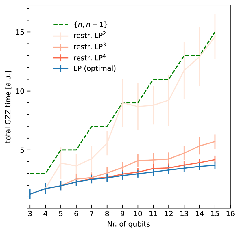
Figure 1: Comparing the performance of the original LP (11) and the restricted LP^j (V) for $j=2,3,4$. The data points and error bars show the mean and variance over $100$ uniformly sampled matrices $A_{ij}=A_{ji}\in[-1,1]$ for $i<j$. The green dashed line is the conjectured upper bound for the original LP (11) from 16 below.

V.1 Numerical benchmark for the heuristic

We compare the performance of the restricted LP^j (V) to the original LP (11). $\operatorname{\mathsf{GZZ}}(A)$ gates with uniformly sampled matrix elements $A_{ij}=A_{ji}\in[-1,1]$ for all $i<j$ and $i,j\in[n]$ are synthesized. For convenience, set $M=A$, i.e. setting $J=E_{n}$ which omits the hardware specific time units given by the quantum platform. For realistic $J$’s and $\operatorname{\mathsf{GZZ}}(A)$ gate times we refer to [7]. The Python package CVXPY [21, 22] with the GNU linear program kit simplex solver [23] is used to solve the LP’s.

Figure 1 shows the total $\operatorname{\mathsf{GZZ}}$ time over the number of qubits for the restricted LP^j (V) and the LP (11). The green dashed line is the upper bound on the total $\operatorname{\mathsf{GZZ}}$ time for the original LP (11) from 16 below. The total $\operatorname{\mathsf{GZZ}}$ time from the restricted LP² seems to scale as this upper bound. Increasing $j>2$ reduces the total $\operatorname{\mathsf{GZZ}}$ time significantly. From Fig. 1 it is observed that the optimal solution of the original LP (11) is well below the conjectured upper bound. We only solved the original LP (11) up to $15$ qubits due to the high runtime.

VI Bounds on the total GZZ time

Our main analytic result (Theorem 15) is that the optimal total $\operatorname{\mathsf{GZZ}}$ time $\boldsymbol{1}^{T}\boldsymbol{\lambda}^{*}$ is lower and upper bounded by the norms $\lVert M\rVert_{\ell_{\infty}}$ and $\lVert M\rVert_{\ell_{1}}$, respectively. Note, that for a dense matrix $M$, its norm $\lVert M\rVert_{\ell_{1}}$ scales quadratic with the number of qubits $n$. We conjecture an improved upper bound on the total $\operatorname{\mathsf{GZZ}}$ time for dense $M$ that scales at most linear with the number of qubits $n$. We support this conjecture with explicit solutions for the LP (11) reaching this bound for any $n$ and numerical results validating the conjecture for $n\leq 8$.

Theorem 15.

The optimal total gate time of $\operatorname{\mathsf{GZZ}}(A)$ with $A\in\operatorname{\mathrm{Sym}_{0}}(\mathbb{R}^{n})$ is lower and upper bounded by

$$\lVert M\rVert_{\ell_{\infty}}\leq\boldsymbol{1}^{T}\boldsymbol{\lambda}^{*}\leq\lVert M\rVert_{\ell_{1}}\,,$$ (37)

where $M\coloneqq A\oslash J$. Equality holds for the lower bound for all matrices $M=C\boldsymbol{m}\boldsymbol{m}^{T}$ for any $\boldsymbol{m}\in\{-1,+1\}^{n}$ and $C\geq 0$.

Proof.

The lower bound has been shown in Lemma 7. Equality in the lower bound holds for $M=C\boldsymbol{m}\boldsymbol{m}^{T}$ by setting $\lambda_{\boldsymbol{m}}=C=\lVert M\rVert_{\ell_{\infty}}$ and $\lambda_{\boldsymbol{m}^{\prime}}=0$ for all $\boldsymbol{m}^{\prime}\neq\boldsymbol{m}$. We use the explicit construction of the standard basis elements for symmetric matrices from the proof of Theorem 14 to show the upper bound. To be precise, we have

$$\frac{|M_{ij}|}{d}(H^{d}_{\boldsymbol{r}})^{T}H^{d}_{\boldsymbol{r}}=M_{ij}e_{(i,j)}\,,$$ (38)

where $\boldsymbol{r}=(i,j)$ if $M_{ij}\geq 0$ or $\boldsymbol{r}=(\tilde{i},\tilde{j})$ if $M_{ij}<0$ as in Eqs. 34 and 35, respectively. We define $\boldsymbol{\lambda}^{(i,j)}$ with the entries $\lambda^{(i,j)}_{\boldsymbol{m}}\coloneqq\frac{|M_{ij}|}{d}\,\delta_{\boldsymbol{m}\in\operatorname{rows}(H^{d}_{\boldsymbol{r}})}$. According to Lemma 8 we have $\boldsymbol{1}^{T}\boldsymbol{\lambda}^{(i,j)}=|M_{ij}|$. Adding $\boldsymbol{\lambda}^{(i,j)}$ for all $i<j$ yields the upper bound $\lVert M\rVert_{\ell_{1}}$. ∎

These bounds get tighter the sparser $M$ is. If $M$ has only one non-zero value, then clearly $\lVert M\rVert_{\ell_{\infty}}=\boldsymbol{1}^{T}\boldsymbol{\lambda}^{*}=\lVert M\rVert_{\ell_{1}}$. Furthermore, these bounds also hold for the heuristic, which we presented in Section V.

Next, we state our conjecture that the optimal gate time of $\operatorname{\mathsf{GZZ}}(A)$ scales at most linear with the number of qubits.

Conjecture 16.

The optimal gate time of $\operatorname{\mathsf{GZZ}}(A)$ with $A\in\operatorname{\mathrm{Sym}_{0}}(\mathbb{R}^{n})$ is tightly upper bounded by

$$\boldsymbol{1}^{T}\boldsymbol{\lambda}^{*}\leq\lVert M\rVert_{\ell_{\infty}}\cdot\begin{cases}n\,,&\text{for odd }n\,,\\ n-1\,,&\text{for even }n\,.\end{cases}$$ (39)

Hence, it provides a tighter bound for dense $M$ than Theorem 15. To support the claim of 16 we first construct explicit dual and primal feasible solutions for the case $M=-E_{n}$ for the LP’s (11) and (II), respectively. Then optimality is given by showing equality of the objective function values of the primal and dual problem. We further show that the case $M=-E_{n}$ leads to the same objective function value as $M=-\boldsymbol{m}\boldsymbol{m}^{T}$ for any $\boldsymbol{m}\in\{-1,1\}^{n}$. Finally, we provide numerical evidence that the conjecture holds for $n\leq 8$.

For practical purposes it is important to keep in mind that the platform given $J$ matrix might also scale with the number of qubits resulting in a qubit dependent constant $\lVert A\oslash J_{n}\rVert_{\ell_{\infty}}=\lVert M_{n}\rVert_{\ell_{\infty}}$.

VI.1 Explicit solutions for $M=-\boldsymbol{m}\boldsymbol{m}^{T}$

The following lemma will be used in the proof of the explicit feasible solution of the dual problem for $M$ being of the form $M=-\boldsymbol{m}\boldsymbol{m}^{T}$. We can identify $\boldsymbol{m}\in\{-1,1\}^{n}$ with $\boldsymbol{b}\in\mathbb{F}_{2}^{n}$ via $\boldsymbol{m}=(-1)^{\boldsymbol{b}}$ as explained in Section II.

Lemma 17.

It holds that

$$P_{\boldsymbol{b}}\coloneqq\sum_{i<j}^{n}(-1)^{b_{i}\oplus b_{j}}=\binom{n}{2}-2|\boldsymbol{b}|(n-|\boldsymbol{b}|)\,,$$ (40)

for any binary vector $\boldsymbol{b}\in\mathbb{F}_{2}^{n}$. We denote the Hamming weight by $|\boldsymbol{b}|$.

Proof.

Let $\boldsymbol{m}=(-1)^{\boldsymbol{b}}$. If the Hamming weight $|\boldsymbol{b}|$ vanishes, then $\boldsymbol{m}=(+1,\dots,+1)$ and $P_{\boldsymbol{b}}=\binom{n}{2}$ which is the maximal value. If $|\boldsymbol{b}|\neq 0$, $\boldsymbol{m}$ contains $|\boldsymbol{b}|$ entries $-1$, such that the upper triangular part of $\boldsymbol{m}\boldsymbol{m}^{T}$ contains a rectangle of $-1$’s with length $|\boldsymbol{b}|$ and width $n-|\boldsymbol{b}|$ so the total amount of $-1$’s is $|\boldsymbol{b}|(n-|\boldsymbol{b}|)$. Therefore,

$$P_{\boldsymbol{b}}=\binom{n}{2}-2|\boldsymbol{b}|(n-|\boldsymbol{b}|)\,.$$ (41)

∎

Lemma 18 (explicit dual feasible solution).

Let $M=-E_{n}$, then there is an explicit feasible solution $\boldsymbol{y}$ to the dual LP (II) with

$$\langle-E_{n},\boldsymbol{y}\rangle=\begin{cases}n\,,&\text{for odd }n\,,\\ n-1\,,&\text{for even }n\,.\end{cases}$$ (42)

Proof.

We assume that $y=y_{1}=y_{2}=\dots$. Therefore, it suffices to show that

$$y\sum_{i<j}^{n}(-1)^{b_{i}\oplus b_{j}}\leq 1\,.$$ (43)

From Lemma 17 we know that $\boldsymbol{y}=1/\operatorname{min}(P_{\boldsymbol{b}})\boldsymbol{1}$ satisfies the constraint in Eq. 43. The minimum $\operatorname{min}(P_{\boldsymbol{b}})=-\lfloor n/2\rfloor$ is reached for $|\boldsymbol{b}|=\lceil n/2\rceil$ or $|\boldsymbol{b}|=\lfloor n/2\rfloor$ which can be verified from the expression of $P_{\boldsymbol{b}}$ in Lemma 17. Thus, we obtain $\boldsymbol{y}=-1/\lfloor n/2\rfloor\boldsymbol{1}$. The objective function evaluates to

$$\langle-E_{n},\boldsymbol{y}\rangle=\boldsymbol{-}\boldsymbol{1}^{T}\boldsymbol{y}=\frac{\binom{n}{2}}{\lfloor n/2\rfloor}=\begin{cases}n\,,&\text{for odd }n\,,\\ n-1\,,&\text{for even }n\,.\end{cases}$$ (44)

∎

For the construction of a feasible solution to the primal problem we first require the following result.

Lemma 19.

Let $k<n$ be natural numbers. Then

$$\sum_{\boldsymbol{b}\in\mathbb{F}_{2}^{n}:|\boldsymbol{b}|=k}|b_{i}\oplus b_{j}|=2\binom{n-2}{k-1}$$ (45)

for all $i,j\in[n]$ with $i\neq j$.

Proof.

Consider the case $n=4$ and $k=2$. We get $\binom{4}{2}=6$ binary vectors with $|\boldsymbol{b}|=2$. It can be easily verified that $\sum_{|\boldsymbol{b}|=2}|b_{i}\oplus b_{j}|=4=2\binom{2}{1}$. Now, we assume that for a given $n$ and $k<n$ the Eq. 45 holds. It suffices to verify Eq. 45 for $i\leq n$ and $j=n+1$. We fix $k$, define $n^{\prime}\coloneqq n+1$ and take a $\boldsymbol{b}\in\mathbb{F}_{2}^{n^{\prime}}$. We have $\binom{n+1}{k}$ binary vectors with $|\boldsymbol{b}|=k$.

For the case $b_{n+1}=0$ we have $\binom{n}{k}$ such vectors and

$$\sum_{\begin{subarray}{c}|\boldsymbol{b}|=k\\ b_{n+1}=0\end{subarray}}|b_{i}\oplus b_{n+1}|=\sum_{|\boldsymbol{b}|=k}|b_{i}|=\binom{n-1}{k-1}\,,$$ (46)

for all $i\leq n$. There are $\binom{n-1}{k-1}$ different ways in placing $k-1$ $1$’s.

For the case $b_{n+1}=1$ we have $\binom{n}{k-1}$ such vectors and

$$\sum_{\begin{subarray}{c}|\boldsymbol{b}|=k\\ b_{n+1}=1\end{subarray}}|b_{i}\oplus b_{n+1}|=\sum_{|\boldsymbol{b}|=k}|b_{i}\oplus 1|=\binom{n-1}{k-1}\,,$$ (47)

for all $i\leq n$. There are $\binom{n-1}{k-1}$ different ways in placing $k-1$ $0$’s.

Combining the two cases $b_{n+1}=0$ and $b_{n+1}=1$ we obtain

$$\sum_{|\boldsymbol{b}|=k}|b_{i}\oplus 0|+|b_{i}\oplus 1|=2\binom{n-1}{k-1}=2\binom{n^{\prime}-2}{k-1}\,,$$ (48)

for all $i\leq n$. ∎

We motivate the next lemma with the result of the explicit dual feasible solution for $M=-E_{n}$ from Lemma 18 and the complementary slackness condition. The complementary slackness condition for a linear program states that if the $i$-th inequality of the dual problem is a strict inequality for a feasible solution $\boldsymbol{y}$, then the $i$-th component of a feasible solution of the primal problem $\boldsymbol{\lambda}$ is zero:

$$(V^{T}\boldsymbol{y})_{i}<1\Rightarrow\lambda_{i}=0\,.$$ (49)

We use this in the following lemma to construct a feasible solution for the primal LP (11).

Lemma 20 (explicit primal feasible solution).

Let $M=-E_{n}$, then there is an explicit feasible solution $\boldsymbol{\lambda}$ to the primal LP (11) with

$$\boldsymbol{1}^{T}\boldsymbol{\lambda}=\begin{cases}n\,,&\text{for odd }n\,,\\ n-1\,,&\text{for even }n\,.\end{cases}$$ (50)

Proof.

For this proof we define

$$k\coloneqq\begin{cases}n\,,&\text{for odd }n\,,\\ n-1\,,&\text{for even }n\,.\end{cases}$$ (51)

We only consider binary vectors of the set $S\coloneqq\left\{\boldsymbol{b}\in\mathbb{F}_{2}^{n}\nonscript\>\middle|\allowbreak\nonscript\>\mathopen{}|\boldsymbol{b}|=\lceil n/2\rceil,\lfloor n/2\rfloor\text{ and }b_{n}=0\right\}$. This set is motivated by the complementary slackness condition and Lemma 18. It can be calculated that $|S|=\binom{k}{\lfloor k/2\rfloor}$ using the recurrence relation

$$\binom{n}{k}=\binom{n-1}{k}+\binom{n-1}{k-1}$$ (52)

for the binomial coefficients. We show that

$$\sum_{\boldsymbol{b}\in S}(-1)^{b_{i}\oplus b_{j}}=-D_{n}\,,$$ (53)

for a constant $D_{n}>0$, which we calculate later. If not explicitly stated, all equations in this proof containing $i$, $j$ hold for all $i,j\in[n]$, $i\neq j$. We denote $\boldsymbol{\lambda}_{S}$ by all $\lambda_{\boldsymbol{m}}=\lambda_{\boldsymbol{b}}$ corresponding to the encoding $\boldsymbol{m}=(-1)^{\boldsymbol{b}}$ with $\boldsymbol{b}\in S$. If Eq. 53 holds, we can choose a $\boldsymbol{\lambda}_{S}=1/D_{n}\boldsymbol{1}$ resulting in

$$\sum_{\boldsymbol{b}\in S}\boldsymbol{\lambda}_{\boldsymbol{b}}(-1)^{b_{i}\oplus b_{j}}=-1\,,$$ (54)

which implies feasibility for $M=-E_{n}$. It is left to show Eq. 53 and determine $D_{n}$.

First, we consider odd $n$. By definition of $S$ we have that $b_{n}=0$ for all $\boldsymbol{b}$. Therefore, we obtain $\binom{n-1}{\lfloor n/2\rfloor}+\binom{n-1}{\lceil n/2\rceil}$ binary vectors with $|\boldsymbol{b}|=\lceil n/2\rceil$ or $|\boldsymbol{b}|=\lfloor n/2\rfloor$ respectively. Counting the occurrences of “$-1$” in the sum of Eq. 53 is equivalent to counting the occurrences of “$1$” in the sum

$$\sum_{\boldsymbol{b}\in S}|b_{i}\oplus b_{j}| =2\left(\binom{n-3}{\lfloor\frac{n}{2}\rfloor-1}+\binom{n-3}{\lceil\frac{n}{2}\rceil-1}\right)$$ (55)

$$=2\binom{n-2}{\lfloor\frac{n}{2}\rfloor}\,,$$

where we used Lemma 19, the recurrence relation for the binomial coefficients and $\lceil n/2\rceil-1=\lfloor n/2\rfloor$. Counting the occurrences of “$+1$” in the sum of Eq. 53 yields

$$\binom{n-1}{\lfloor\frac{n}{2}\rfloor}+\binom{n-1}{\lceil\frac{n}{2}\rceil}-2\binom{n-2}{\lfloor\frac{n}{2}\rfloor}=\binom{n}{\lfloor\frac{n}{2}\rfloor}-2\binom{n-2}{\lfloor\frac{n}{2}\rfloor}\,.$$ (56)

where we used $\binom{n}{\lfloor n/2\rfloor+1}=\binom{n}{\lfloor n/2\rfloor}$ for odd $n$. We now evaluate Eq. 53 for odd $n$

$$-D_{n}=\sum_{\boldsymbol{b}\in S}(-1)^{b_{i}\oplus b_{j}} =\binom{n}{\lfloor\frac{n}{2}\rfloor}-4\binom{n-2}{\lfloor\frac{n}{2}\rfloor}$$ (57)

$$=\binom{n}{\lfloor\frac{n}{2}\rfloor}-\frac{n+1}{n}\binom{n}{\lfloor\frac{n}{2}\rfloor}$$

$$=\frac{-1}{n}\binom{n}{\lfloor\frac{n}{2}\rfloor}\,.$$

The case for even $n$ follows the same steps as for odd $n$, resulting in

$$-D_{n}=\sum_{|\boldsymbol{b}|=\frac{n}{2}}(-1)^{b_{i}\oplus b_{j}} =\binom{n-1}{\frac{n}{2}}-\frac{n}{n-1}\binom{n-1}{\frac{n}{2}}$$ (58)

$$=\frac{-1}{n-1}\binom{n-1}{\frac{n}{2}}\,.$$

Equations 57 and 58 show that $D_{n}=1/k\binom{k}{\lfloor k/2\rfloor}$ and that Eq. 53 holds. Since $|S|=\binom{k}{\lfloor k/2\rfloor}$ the objective function value is

$$\boldsymbol{1}^{T}\boldsymbol{\lambda}_{S}=\binom{k}{\lfloor k/2\rfloor}\frac{1}{\frac{1}{k}\binom{k}{\lfloor k/2\rfloor}}=k\,.$$ (59)

∎

From the equality of the objective functions for the primal and dual problem from Lemma 20 and Lemma 18 respectively we know that the proposed dual/primal feasible solutions for $M=-E_{n}$ are in fact optimal solutions. Now, we show that the $\operatorname{\mathsf{GZZ}}$ gate time with $M=-\boldsymbol{m}\boldsymbol{m}^{T}$ for any $\boldsymbol{m}\in\{-1,+1\}^{n}$ is the same as for the case $M=-E_{n}$.

Theorem 21.

If $A\oslash J\eqqcolon M=-C(\boldsymbol{m}\boldsymbol{m}^{T})$ for any $\boldsymbol{m}\in\{-1,+1\}^{n}$ and $C\geq 0$, then the optimal gate time of $\operatorname{\mathsf{GZZ}}(A)$ is

$$\boldsymbol{1}^{T}\boldsymbol{\lambda}^{*}=\lVert M\rVert_{\ell_{\infty}}\begin{cases}n\,,&\text{for odd }n\,,\\ n-1\,,&\text{for even }n\,.\end{cases}$$ (60)

Proof.

The statement has been shown for the case $M=-E_{n}$ by constructing an explicit solution. It is left to show that the cases $M=-C(\boldsymbol{m}\boldsymbol{m}^{T})$ for a constant $C\geq 0$ yield the same objective function value. Since the objective function and the constraints are linear we can w.l.o.g. assume $C=1$. It is clear, that $\operatorname{sign}(M_{ij})=\operatorname{sign}(-m_{i}m_{j})=-(-1)^{c_{i}\oplus c_{j}}$ for all $i<j$, with $\boldsymbol{m}=(-1)^{\boldsymbol{c}}$. Let $\boldsymbol{y}=-y\operatorname{sign}(\boldsymbol{v}(M))$ for a $y\in\mathbb{R}$, then each constraint of $V^{T}\boldsymbol{y}\leq\boldsymbol{1}$ of the dual LP (II) reads as

$$y\sum_{i<j}(-1)^{b_{i}\oplus b_{j}\oplus c_{i}\oplus c_{j}}=y\sum_{i<j}(-1)^{\tilde{b}_{i}\oplus\tilde{b}_{j}}\leq 1\,,$$ (61)

with $\boldsymbol{\tilde{b}}\coloneqq\boldsymbol{b}\oplus\boldsymbol{c}$ element wise. Consider the ordered set of all $\boldsymbol{b}\in\mathbb{F}_{2}^{n}$ with $b_{n}=0$, then $\boldsymbol{\tilde{b}}$ is just a permutation of that set. Due to the permutation symmetry of the qubits the optimal value of the LP (11) for any $M=-(\boldsymbol{m}\boldsymbol{m}^{T})$ is the same as for the case $M=-E_{n}$. Setting $\boldsymbol{y}=-y\operatorname{sign}(\boldsymbol{v}(M))$ with $y=1/\lfloor n/2\rfloor$ as in the proof of Lemma 18 yields an optimal solution to the dual LP (II) for the case $M=-(\boldsymbol{m}\boldsymbol{m}^{T})$. ∎

Note that, trivially, the lower bound $\boldsymbol{1}^{T}\boldsymbol{\lambda}^{*}=\lVert M\rVert_{\ell_{\infty}}$ is reached if $M=C(\boldsymbol{m}\boldsymbol{m}^{T})$ for any $\boldsymbol{m}\in\{-1,+1\}^{n}$ and $C\geq 0$.

One possibility to prove 16 is to show, that the matrix $M=-E_{n}$ maximizes the value of the LP (11) among all matrices $M\in\operatorname{\mathrm{Sym}_{0}}([-1,+1]^{n})$. To this end, consider the LP ∥ y ∥_ℓ_1 V^T y ≤1 y∈R^(n2)   , which is independent of $M\in\operatorname{\mathrm{Sym}_{0}}([-1,+1]^{n})$. It holds that

$$\max_{V^{T}\boldsymbol{y}\leq\boldsymbol{1}}\left(\max_{\lVert M\rVert_{\ell_{\infty}}\leq 1}\langle M,\boldsymbol{y}\rangle\right)=\max_{V^{T}\boldsymbol{y}\leq\boldsymbol{1}}\lVert\boldsymbol{y}\rVert_{\ell_{1}}$$ (62)

according to $\lVert\boldsymbol{x}\rVert_{\ell_{1}}=\max_{\lVert\boldsymbol{p}\rVert_{\ell_{\infty}}\leq 1}\boldsymbol{p}^{T}\boldsymbol{x}$. Therefore, the optimal objective value of LP (21) is an upper bound on all optimal objective values of LP (11). Clearly, the constructed solution in Lemma 18 is feasible for LP (21). Unfortunately, proving that this constructed solution is optimal is quite challenging, as we discuss in Appendix A.

VI.2 Numeric validation of the conjecture for small $n$

For the numeric validation of the conjecture for small $n$ we solve the dual LP (II) for all binary $M\in\operatorname{\mathrm{Sym}_{0}}(\{-1,+1\}^{n})$ of which there are $2^{\binom{n}{2}}$. For $n=3$ there are only binary matrices of the form $M=\pm(\boldsymbol{m}\boldsymbol{m}^{T})$ and by Theorem 21 the conjecture holds. Figure 2 shows that 16 holds for $n\leq 8$. For odd $n\leq 8$ the cases $M=-(\boldsymbol{m}\boldsymbol{m}^{T})$ are in fact the only cases reaching the upper bound. This can be seen in Fig. 2 by the blue area exceeding the orange area, which only consists of the optimal values for all binary matrices without $M=\pm(\boldsymbol{m}\boldsymbol{m}^{T})$ for any $\boldsymbol{m}\in\{-1,+1\}^{n}$.

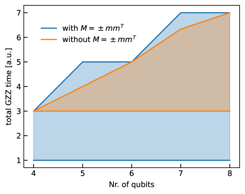
Figure 2: The optimal objective function value of the dual LP (II) over the number of qubits. Blue: The range of optimal values for all binary $M\in\operatorname{\mathrm{Sym}_{0}}(\{-1,+1\}^{n})$. Orange: The range of optimal values for all binary $M\in\operatorname{\mathrm{Sym}_{0}}(\{-1,+1\}^{n})$ without $M=\pm(\boldsymbol{m}\boldsymbol{m}^{T})$ for any $\boldsymbol{m}\in\{-1,+1\}^{n}$.

VII Conclusion

We investigated the time-optimal multi-qubit gate synthesis introduced in Ref. [7]. We show that synthesizing time-optimal multi-qubit gates in our setting is $\mathsf{NP}$-hard. However, we also provide explicit solutions for certain cases with constant gate time and a polynomial-time heuristics to synthesize fast multi-qubit gates. Our numerical simulations suggest that these heuristics provide good approximations to the optimal $\operatorname{\mathsf{GZZ}}$ gate time. Furthermore, tight bounds on the scaling of the optimal multi-qubit gate times were shown. More precisely, we showed that the optimal multi-qubit gate time scales at most as $\lVert A\oslash J\rVert_{\ell_{1}}$, the $\ell_{1}$-norm of the element-wise division of the total and physical coupling matrices $A$ and $J$, respectively. We also conjectured that the optimal $\operatorname{\mathsf{GZZ}}$ gate time scales at most linear with the number of qubits. Our results are practical to estimate the execution time of a given circuit, where the entangling gates are implemented as $\operatorname{\mathsf{GZZ}}$ gates. The execution time is a crucial parameter, in particular, in the NISQ era since it is limiting the length of a gate sequence due to finite coherence time.

It is our hope to proof the conjectured linear scaling of the optimal $\operatorname{\mathsf{GZZ}}$ gate time in the near future. Moreover, we would like to test and verify our proposed time-optimal multi-qubit gate synthesis methods in an experiment. Depending on the quantum platform we would like to develop adapted error mitigation schemes for the $\operatorname{\mathsf{GZZ}}$ gates and investigate their robustness against errors.

Appendices

Appendix A Challenges in proving Conjecture 16

In this section, we want to discuss some obstacles encountered trying to proof 16. 16 holds, if we show that our constructed solutions from Section VI.1 are optimal solutions for LP (21). Meaning that there is no other feasible solution resulting in a larger objective function value compared to our constructed solution.

We tried an inductive proof which turned out to be intricate due to the additional degrees of freedom in each induction step. Furthermore, we utilized the connection to graph theory from Lemma 2 to transform the LP (21) to a LP over the cut polytope. There, the challenge is the affine mapping between the elliptope and the cut polytope in Eq. 12 and Definition 1, which alters the optimization problem crucially. In the following, we discuss another approach based on showing the sufficiency of the Karush–Kuhn–Tucker (KKT) conditions in more detail.

A.1 Concave program

A convex linear program in standard form minimizes a convex objective function over a convex set. But LP (21) maximizes a convex objective function over a convex set. Such optimizations are called concave programs. It is known that the maximum is attained at the extreme points of the polytope $V^{T}\boldsymbol{y}\leq\boldsymbol{1}$ and therefore might have many local optima [24]. There are several equivalent sufficient conditions for optimality [25]. Here, we investigate one in detail. First, we define the conjugate function for a function $f:\mathbb{R}^{n}\rightarrow\mathbb{R}$

$$f^{*}(\boldsymbol{x})\coloneqq\sup\left\{\boldsymbol{x}^{T}\boldsymbol{y}-f(\boldsymbol{y})\nonscript\>\middle|\allowbreak\nonscript\>\mathopen{}\boldsymbol{y}\in\mathcal{D}(f)\right\}\,,$$ (63)

with $\mathcal{D}(f)$ the domain of $f$. Furthermore, we need the support function $h_{A}:\mathbb{R}^{n}\rightarrow\mathbb{R}$ for a closed convex set $A$

$$h_{A}(\boldsymbol{x})\coloneqq\sup\left\{\boldsymbol{x}^{T}\boldsymbol{y}\nonscript\>\middle|\allowbreak\nonscript\>\mathopen{}\boldsymbol{y}\in A\right\}\,.$$ (64)

Then the sufficient optimality condition in our case is

$$\lVert\boldsymbol{y}^{*}\rVert_{\ell_{1}}=\sup\left\{h_{A}(\boldsymbol{x})-(\lVert\boldsymbol{x}\rVert_{\ell_{1}})^{*}\nonscript\>|\allowbreak\nonscript\>\mathopen{}\boldsymbol{y}\in\mathbb{R}^{\binom{n}{2}}\right\}\,,$$ (65)

with $A=\left\{\boldsymbol{x}\in\mathbb{R}^{\binom{n}{2}}\nonscript\>\middle|\allowbreak\nonscript\>\mathopen{}V^{T}\boldsymbol{x}\leq\boldsymbol{1}\right\}$. The conjugate function of $\lVert\boldsymbol{x}\rVert_{\ell_{1}}$ is

$$(\lVert\boldsymbol{x}\rVert_{\ell_{1}})^{*}=\begin{cases}0\,,&\text{if }\lVert\boldsymbol{x}\rVert_{\ell_{\infty}}\leq 1\,,\\ \infty\,,&\text{otherwise}\,.\end{cases}$$ (66)

Then we have

$$\lVert\boldsymbol{y}^{*}\rVert_{\ell_{1}} =\sup\left\{h_{A}(\boldsymbol{y})\nonscript\>\middle|\allowbreak\nonscript\>\mathopen{}\lVert\boldsymbol{y}\rVert_{\ell_{\infty}}\leq 1\right\}$$ (67)

$$=\sup\left\{\boldsymbol{x}^{T}\boldsymbol{y}\nonscript\>\middle|\allowbreak\nonscript\>\mathopen{}\lVert\boldsymbol{y}\rVert_{\ell_{\infty}}\leq 1,V^{T}\boldsymbol{x}\leq\boldsymbol{1}\right\}$$

$$=\sup\left\{\lVert\boldsymbol{x}\rVert_{\ell_{1}}\nonscript\>|\allowbreak\nonscript\>\mathopen{}V^{T}\boldsymbol{x}\leq\boldsymbol{1}\right\}\,,$$

which is the same formulation as the original LP (21).

A.2 Dualization

If we can formulate the dual LP to the primal LP (21) and find a feasible solution, then the dual objective function value upper bounds the primal objective function value by weak duality [26]. The standard form of an optimization problem with only linear inequality constraints is f(y) A y ≤b. Then, the Lagrange dual function is given by

$$g(\boldsymbol{\lambda})=-\boldsymbol{b}^{T}\boldsymbol{\lambda}-f^{*}(-A^{T}\boldsymbol{\lambda})\,,$$ (68)

where $f^{*}$ denotes the conjugate function [10]. For LP (21) we have $f(\boldsymbol{y})=-\lVert\boldsymbol{y}\rVert_{\ell_{1}}$ (minus sign due to the minimization in the standard optimization form).

$$(-\lVert\boldsymbol{x}\rVert_{\ell_{1}})^{*} =\sup\left\{\boldsymbol{x}^{T}\boldsymbol{y}+\lVert\boldsymbol{x}\rVert_{\ell_{1}}\nonscript\>|\allowbreak\nonscript\>\mathopen{}\boldsymbol{y}\in\mathbb{R}^{\binom{n}{2}}\right\}$$ (69)

$$=\sup\left\{\boldsymbol{x}^{T}\boldsymbol{y}+\boldsymbol{x}^{T}\boldsymbol{z}\nonscript\>\middle|\allowbreak\nonscript\>\mathopen{}\boldsymbol{y}\in\mathbb{R}^{\binom{n}{2}},\lVert\boldsymbol{z}\rVert_{\ell_{\infty}}\leq 1\right\}$$

$$=\sup\left\{\boldsymbol{x}^{T}\boldsymbol{y}\nonscript\>\middle|\allowbreak\nonscript\>\mathopen{}\boldsymbol{y}\in\mathbb{R}^{\binom{n}{2}}\right\}\,,$$

which clearly is unbounded if $\boldsymbol{x}\neq\boldsymbol{0}$. Therefore, we cannot formulate the dual to LP (21).

A.3 Invexity

The KKT conditions are optimality conditions for non-linear optimization problems. Invexity is a generalization of convexity in the sense that the KKT conditions are necessary and sufficient for optimality [27]. By invexity we mean that the objective and constraint functions of the optimization problem are Type 1 invex functions.

Definition 22.

Consider the standard form of an optimization problem f(y) g( y ) ≤0 y ∈S, where $\mathcal{S}\subseteq\mathbb{R}^{m}$ is defined by $g(\boldsymbol{y})\leq\boldsymbol{0}$. Then $f$ and $g$ are called Type 1 invex functions at point $\boldsymbol{y}^{*}\in\mathcal{S}$ w.r.t. a common function $\eta(\boldsymbol{y},\boldsymbol{y}^{*})\in\mathbb{R}^{m}$, if for all $\boldsymbol{y}\in\mathcal{S}$,

$$f(\boldsymbol{y})-f(\boldsymbol{y}^{*}) \geq\eta(\boldsymbol{y},\boldsymbol{y}^{*})^{T}\nabla f(\boldsymbol{y}^{*}),$$ (70)

$$-g(\boldsymbol{y}^{*}) \geq\eta(\boldsymbol{y},\boldsymbol{y}^{*})^{T}\nabla g(\boldsymbol{y}^{*})$$

hold. It suffices to consider only the active constraints, i.e. the constraints, where equality holds $g(\boldsymbol{y}^{*})=0$. [27]

Let $K$ be the scaling factor of the conjectured upper bound, i.e.

$$K\coloneqq\begin{cases}n\,,&\text{for odd }n\,,\\ n-1\,,&\text{for even }n\,.\end{cases}$$ (71)

In the case of LP (21) we have $\mathcal{S}=\left\{\boldsymbol{y}\in\mathbb{R}^{\binom{n}{2}}\nonscript\>\middle|\allowbreak\nonscript\>\mathopen{}V^{T}\boldsymbol{y}\leq\boldsymbol{1}\right\}$ and want to show that $\boldsymbol{y}^{*}=-\boldsymbol{1}/\lfloor n/2\rfloor$ is a global optimum. Furthermore, we have

$$f(\boldsymbol{y}) =-\lVert\boldsymbol{y}\rVert_{\ell_{1}}\,,\hskip 9.49997ptf(\boldsymbol{y}^{*})=-K\,,\,\,\nabla f(\boldsymbol{y}^{*})=\boldsymbol{1}\,,$$ (72)

$$g(\boldsymbol{y}) =V^{T}\boldsymbol{y}-\boldsymbol{1}\,,\,\,g(\boldsymbol{y}^{*})=0\,,\hskip 16.49995pt\nabla g(\boldsymbol{y}^{*})=V|_{a}\,,$$

where $V|_{a}$ are the columns of $V$ such that $(V|_{a})^{T}\boldsymbol{y}^{*}=\boldsymbol{1}$, i.e. the active constraints. To show invexity we have to find a common $\eta(\boldsymbol{y},\boldsymbol{y}^{*})\in\mathbb{R}^{m}$ such that

$$\lVert\boldsymbol{y}\rVert_{\ell_{1}} \leq K-\eta^{T}(\boldsymbol{y},\boldsymbol{y}^{*})\boldsymbol{1}\,\text{ and}$$ (73)

$$(V^{T}|_{a})\eta(\boldsymbol{y},\boldsymbol{y}^{*}) \leq\boldsymbol{0}\,,$$

for all $\boldsymbol{y}\in\mathcal{S}$. It is quite challenging to find a $\eta(\boldsymbol{y},\boldsymbol{y}^{*})\in\mathbb{R}^{m}$ satisfying both inequalities. In particular, ansätze motivated from the geometry in small dimensions eventually fail for larger $n$.

Appendix B Acronyms