LMU–ASC 25/23

Scale invariant Einstein-Cartan gravity
and flat space conformal symmetry

Georgios K. Karananas,^⋆ Mikhail Shaposhnikov,^† Sebastian Zell ^‡

^⋆Arnold Sommerfeld Center
Ludwig-Maximilians-Universität München
Theresienstraße 37, 80333 München, Germany
^†Institute of Physics
École Polytechnique Fédérale de Lausanne (EPFL)
CH-1015 Lausanne, Switzerland
^‡Centre for Cosmology, Particle Physics and Phenomenology – CP3,
Université catholique de Louvain,
B-1348 Louvain-la-Neuve, Belgium

georgios.karananas@physik.uni-muenchen.de
mikhail.shaposhnikov@epfl.ch
sebastian.zell@uclouvain.be

We find the conditions under which scale-invariant Einstein-Cartan gravity with scalar matter fields leads to an approximate conformal invariance of the flat space particle theory up to energies of the order of the Planck mass. In the minimal setup, these models, in addition to the fields of the Standard Model and the graviton, contain only one extra particle – a massless dilaton. Theories of this type can pave the way for a self-completion all the way up the Planck scale and lead to rather universal inflationary predictions, close to those of the simplest Higgs-inflation scenario in the metric theory of gravity.

1 Introduction

In [1] we constructed a class of phenomenologically viable theories based on the Einstein-Cartan (EC) gravity [2, 3, 4, 5, 6, 7, 8] which enjoy exact but spontaneously broken scale invariance. These theories, in addition to the Standard Model (SM) and graviton fields, contain just one additional particle – a massless dilaton, being the Nambu-Goldstone (NG) boson of this symmetry. The classical action of these theories is selected with the use of systematic requirements that aim at capturing the minimal ambiguity inevitably contained in General Relativity (GR) [9]. This is achieved by demanding equivalence to the metric formulation of GR in the absence of matter while at the same time avoiding assumptions as far as possible (see [9, 1, 10, 11] for detailed discussions). The criteria of [9] can be expressed as follows [11]:

• The action is polynomial with respect to all matter fields and curvature invariants.

• The action must not contain operators with more than two derivatives (where torsion counts as one derivative).

• The theory should be scale-invariant and thus only contain dimensionless parameters.

In the algebraic flat spacetime limit defined as $e_{\mu}^{A}=\delta_{\mu}^{A},~{}\omega_{\mu}^{AB}=0$, conditions i) - iii) imply that the theory enjoys not only scale-invariance but a wider symmetry – invariance under the 15-parameter full conformal group.

The physical low-energy limit (we stress that this is not the same as the algebraic flat spacetime limit defined above) of these theories is derived by integrating out the non-dynamical torsion and going to the Einstein frame, such that the (canonical) graviton is disentangled from the scalar degrees of freedom. The resulting physical particle physics action is found by dropping the Einstein-Hilbert term and making the metric flat; in general, it is a non-polynomial function of the scalar fields. This action captures the dynamics of a scale invariant theory, where this symmetry is broken spontaneously (realized nonlinearly). For different aspects of this construction, such as quantum corrections, its cosmology and phenomenology, see e.g. [12, 13, 14, 15, 16, 17, 18, 19, 20, 21, 22, 23, 24, 25, 26, 27, 28, 29, 30, 31, 32, 33, 34, 35, 36, 37, 38, 39, 40, 41, 42, 43, 44, 45, 46, 47, 48, 49, 50, 51, 52, 53, 54, 55, 56, 57, 58, 59, 1] for a far-from-complete list of relevant works.

The fact that the resulting particle physics theory for arbitrary choice of different non-minimal couplings to gravity is only scale, but not conformally invariant means that the interaction of the scalar degree of freedom hidden in the metric (or in the vierbein and connection if we talk about EC gravity) breaks explicitly the conformal invariance.

The aim of the present work is to single out the subclass of the theories defined by i) - iii) by adding an extra requirement: the resulting physical theory for energies up to the Planck scale should approximately be conformally invariant rather than only being scale invariant. We note here that it does not make much sense to require the existence of exact conformal symmetry for all energies, since irrespectively of nonminimal coupling(s), the mere existence of gravitational interactions is in conflict [60, 61] with having this symmetry in the physical low-energy limit due to the Weyl anomaly (for a review see [62]). With the use of the language of effective field theories, the physical action of the theory constructed along the lines above is required to read as

$$S_{\rm eff}=S_{\rm conf}+\sum_{n=2}^{\infty}\frac{1}{\Lambda_{\rm conf}^{n}}S_{\rm scale}^{(n)}\ .$$ (1.1)

The first term $S_{\rm conf}$ is essentially a non-polynomial conformally invariant action with the symmetry nonlinearly realized, while the breaking pieces $S_{\rm scale}^{(n)}$ are suppressed by powers of the scale $\Lambda_{\rm conf}$. For reasons that will become clear shortly, we shall take $\Lambda_{\rm conf}=M_{P}$ (it is assumed that the dimensionless coefficients appearing in $S_{\rm scale}^{(n)}$ are of the order of one).

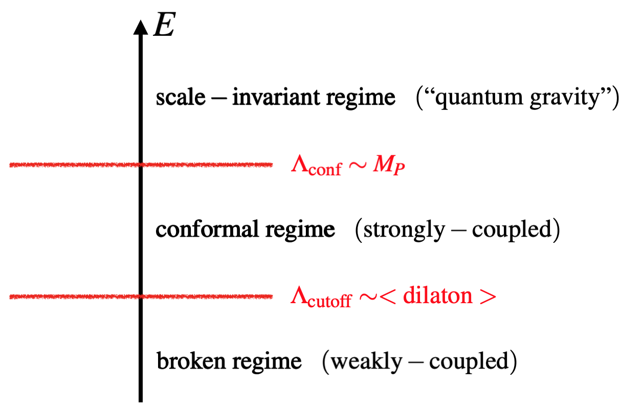
Figure 1: The phase portrait of the theory.

Our interest in this class of theories stems from various field-theoretical as well as phenomenological considerations, on which we elaborate now.

First, theories with exact conformal invariance (CFT’s) exhibit ultraviolet (UV) fixed points in the renormalization group running and are UV complete (for a review see [63]). As already mentioned, the action $S_{\rm conf}$, to be constructed in what follows, is non-polynomial and thus non-renormalizable. As such, it has an intrinsic dimensionful parameter $\Lambda_{\rm cutoff}$ (related to the dilaton vev) which can in principle be much smaller than the Planck scale. If there were no “hidden” conformal symmetry, one would expect that the theory defined by $S_{\rm conf}$ requires some sort of UV completion around the vicinity of $\Lambda_{\rm cutoff}$ with new degrees of freedom showing up at these energies. It is plausible that the conformal symmetry improves the situation, i.e., the theory may “self-complete” in the energy interval $\Lambda_{\rm cutoff}<E\lesssim\Lambda_{\rm conf}$, entering a strongly-coupled conformal regime described by an unbroken CFT.

Second, there are arguments that the requirement of unitarity applied to quantum field theory in flat spacetime excludes theories with scale but no conformal invariance [64]. Taken at face value, this would mean that if the energy scale $\Lambda_{\rm conf}$ around which conformal symmetry is explicitly broken down to scale symmetry is much smaller than $M_{P}$, $\Lambda_{\rm conf}\ll M_{P}$, then the physical action (1.1) as well as the initial action defined by the requirements i) - iii) would not make sense for energies exceeding $\Lambda_{\rm conf}$. Even the part of the theory without gravity should be modified in the energy interval $\Lambda_{\rm conf}<E<M_{P}$, probably by integrating-in new physics. If on the contrary $\Lambda_{\rm conf}\simeq M_{P}$, then the theory merges (in some way) with gravity respecting only the scale-symmetry. The region of validity of (1.1) extends all the way to the Planck scale, and thus no new degrees of freedom are required until such energies. Arguably, this is a rather non-trivial expectation. It remains to be seen if it is true.

For clarity let us recapitulate how we envisage the behavior of the theories under consideration from a bottom-up perspective; see also fig. 1 for a graphical account. At energies below the dilaton expectation value, i.e. for $E\lesssim\Lambda_{\rm cutoff}$, the theory is in its weekly-coupled regime, with conformal symmetry spontaneously broken and the accompanying massless dilaton present. For higher energies, $\Lambda_{\rm cutoff}<E\lesssim\Lambda_{\rm conf}\sim M_{P}$, the theory is in a strongly-coupled regime with restored conformal symmetry and thus becomes a full-blown CFT. Finally, gravity kicks in at $E\sim M_{P}$, explicitly violating conformality but preserving scale-invariance.

In addition to the field-theoretical arguments presented so far, the third and final motivation for investigating aspects of such theories comes from cosmological phenomenology. Without the requirement of approximate conformal invariance up to the Planck scale, theories constructed according to the criteria i) to iii)(or even without the requirement of scale-invariance) contain numerous a priori unknown coupling constants and generically it becomes impossible to derive unique observable predictions [65, 66, 67, 9, 1]. We find indications that approximate conformal symmetry improves the situation considerably: in the context of inflationary model building, we therefore conjecture that primordial observables become nearly universal and close to the ones of single-field Higgs inflation in the metric formulation of General Relativity [68]. As an additional bonus, this leads to excellent agreement with observations [69, 70]. As a proof of concept we provide a concrete example and we leave a detailed investigation for future work.

This article is organized as follows. In Sec. 2, we review briefly well-known facts associated with the constraints conformal symmetry imposes on the action of a real scalar field. In Sec. 3, we generalize these findings to the case of $N$ real scalar fields. The fact that conformal symmetry is more restrictive than scale symmetry becomes apparent already at the level of two derivatives: the kinetic sector is fixed in a rather nontrivial manner—this is to be contrasted with the single field case, where to see such differences one needs to go to the fourth order in the derivatives of the field. We also show that nonlinearly realized conformal symmetry, that is when scales are generated, also constrains the $N$-field action nontrivially. In Sec. 4, we discuss how the explicit breaking of conformal symmetry that goes hand-in-hand with the inclusion of (dynamical) gravity manifests itself at the level of the action. In Sec. 5, we conjecture that flat-space conformality (together with requiring agreement with observations) is powerful enough to make the various Higgs-dilaton models almost indistinguishable from single-field metric Higgs inflation scenario as far as inflationary predictions are concerned. In Sec. 6, we summarize our findings and conclude. Appendix A discusses how the inflationary dynamics are altered once the selection criteria i) - iii) are relaxed.

2 An invitation: a single real scalar field

In this section, we shall discuss well-known facts (see e.g. [71, 72]) about how linearly realized invariance under the full conformal group completely fixes the action of a real scalar field. We do that in two different approaches: algebraic and geometric. In the former, one writes down the most general action involving a scalar and then investigates how it is constrained by requiring that it be invariant under the conformal variation of the field. In the latter, one “dresses” the Minkowski metric with a scalar field and then takes the action to be a derivative expansion of diffeomorphism-invariant objects constructed out of this conformally flat metric with arbitrary coefficients. The following discussion is straightforward and contains nothing new, but we include it for the sake of making the article as self-contained as possible.

2.1 Algebraic approach

Consider a real scalar field $\varphi$ with scaling dimension $\Delta_{\varphi}\neq 0$ in a $D>2$ dimensional  Minkowski spacetime with metric $\eta_{\mu\nu}={\rm diag}(-1,1,\ldots,1)$. We take the action to contain terms that are at most quadratic in the derivatives of the field,

$$S=-\int\!\mathrm{d}^{D}x~{}\left[\frac{1}{2}G(\varphi)(\partial_{\mu}\varphi)^{2}+V(\varphi)\right]\ ,$$ (2.1)

with $G(\varphi)$ and $V(\varphi)$ arbitrary functions. Note that noncanonical kinetic terms appear naturally whenever gravity enters the picture, being the aftermath of nonminimal coupling(s).

Since $\varphi$ is the only dimensionful quantity (apart from $\partial_{\mu}$), it follows from requiring invariance under dilatations only—equivalently by performing dimensional analysis—that

$$V(\varphi)=\tilde{c}\varphi^{\frac{D}{\Delta_{\varphi}}}\ ,~{}~{}~{}\tilde{c}={\rm constant}\ ,$$ (2.2)

as well as

$$G(\varphi)=c\varphi^{\alpha}\ ,~{}~{}~{}c={\rm constant}\ ,$$ (2.3)

where

$$\alpha=-\frac{2}{\Delta_{\varphi}}\left(\Delta_{\varphi}-\frac{D}{2}+1\right)\ .$$ (2.4)

Plugging these results into $S$, we end up with

$$S=-\int\!\mathrm{d}^{D}x\left[\frac{1}{2}c\varphi^{\alpha}(\partial_{\mu}\varphi)^{2}+\tilde{c}\varphi^{\frac{D}{\Delta_{\varphi}}}\right]\ .$$ (2.5)

Next, we study the constraints imposed upon the action (2.1) by requiring that it be conformally invariant, i.e. for $S$ to have a vanishing conformal variation

$$\delta_{c}S=\int\!\mathrm{d}^{D}x\,\frac{\delta S}{\delta\varphi}\delta_{c}\varphi=0\ ,$$ (2.6)

with

$$\delta_{c}\varphi=-\left(\epsilon^{\mu}\partial_{\mu}\varphi+\frac{\Delta_{\varphi}}{D}\varphi\partial_{\mu}\epsilon^{\mu}\right)\ .$$ (2.7)

Here $\epsilon^{\mu}$ is the conformal Killing vector (more details may for instance be found in [73, 63])

$$\epsilon^{\mu}=a^{\mu}+\omega^{\mu}_{\ \nu}x^{\nu}+cx^{\mu}+2(b\cdot x)x^{\mu}-x^{2}b^{\mu}\ ,$$ (2.8)

where $a^{\mu},\omega_{\mu\nu}=-\omega_{\nu\mu},c$ and $b^{\mu}$ are constant parameters associated with translations, Lorentz transformations, dilatations and special conformal transformations, respectively; Eq. (2.8) is the solution to the flat spacetime conformal Killing equation

$$\partial_{\mu}\epsilon_{\nu}+\partial_{\nu}\epsilon_{\mu}=\frac{2}{D}\eta_{\mu\nu}\partial_{\lambda}\epsilon^{\lambda}\ .$$ (2.9)

A straightforward computation shows that

$$\delta_{c}S = -\int\!\mathrm{d}^{D}x\Bigg{[}\frac{1}{2}G^{\prime}(\varphi)\delta_{c}\varphi(\partial_{\mu}\varphi)^{2}+G(\varphi)\partial_{\mu}\varphi\partial^{\mu}\delta_{c}\varphi+V^{\prime}(\varphi)\delta_{c}\varphi\Bigg{]}$$ (2.10)

$$= \int\!\mathrm{d}^{D}x\Bigg{\{}\frac{\partial_{\nu}\epsilon^{\nu}}{D}\Bigg{[}\left(\left(\Delta_{\varphi}-\frac{D}{2}+1\right)G(\varphi)+\frac{\Delta_{\varphi}}{2}\varphi G^{\prime}(\varphi)\right)\partial_{\mu}\varphi\partial^{\mu}\varphi$$

$$+ DV(\varphi)-\Delta_{\varphi}\varphi V^{\prime}(\varphi)\Bigg{]}-\frac{\Delta_{\varphi}}{2D}\partial^{\mu}\partial_{\nu}\epsilon^{\nu}\varphi^{2}G^{\prime}(\varphi)\partial_{\mu}\varphi\Bigg{\}}\ ,$$

where we arranged the terms with increasing powers of derivatives acting on the conformal Killing vector $\epsilon_{\mu}$. For the potential, we notice that it is fixed to be a homogeneous function of the field

$$V(\varphi)=\frac{\Delta_{\varphi}}{D}\varphi V^{\prime}(\varphi)\ .$$ (2.11)

which is automatically fulfilled due to dimensional analysis, as follows from eq. (2.2). We make an analogous observation with regard to the non-canonical coefficient of the kinetic term. Because of eq. (2.3), the last term in (2.10) becomes a total derivative, which can be immediately verified by using the fact that $\epsilon$ is at most quadratic in $x$. Then it follows from eq. (2.4) that the remaining contributions involving $G(\varphi)$ vanish in eq. (2.10). This shows that in the case of a single field, conformal invariance follows automatically from scale invariance.

Finally, one may make the kinetic term of the field in the action (2.5) canonical by introducing

$$\bar{\varphi}=\frac{2\sqrt{c}\Delta_{\varphi}}{D-2}\varphi^{\frac{D-2}{2\Delta_{\varphi}}}\ ,$$ (2.12)

such that

$$\bar{S}=-\int\!\mathrm{d}^{D}x\left[\frac{1}{2}(\partial_{\mu}\bar{\varphi})^{2}+\frac{D-2}{2D}\lambda\bar{\varphi}^{\frac{2D}{D-2}}\right]\ ,$$ (2.13)

with

$$\lambda=\frac{2D}{D-2}\tilde{c}\left(\frac{D-2}{2\sqrt{c}\Delta_{\varphi}}\right)^{\frac{2D}{D-2}}\ .$$ (2.14)

We remark that a canonical kinetic term immediately translates into $\bar{\varphi}$ having canonical scaling dimension too, i.e.

$$\Delta_{\bar{\varphi}}=\frac{D}{2}-1\ ,$$ (2.15)

as it may be verified from its definition eq. (2.12).

2.2 Geometric approach

We can equivalently obtain the same action by utilizing the standard trick of first identifying the field with the scalar mode of a conformally flat metric and then writing down the invariants at each order in derivatives with arbitrary coefficients, see for instance [74, 75, 76, 72].

Since our purpose here is to only get terms at most quadratic in derivatives of the field, our action comprises two terms and reads

$$S=-\int\!\mathrm{d}^{D}x\sqrt{H}\left(\frac{c\Delta_{\varphi}^{2}}{2(D-1)(D-2)}M^{D-2}{\mathcal{R}[H]}+\tilde{c}M^{D}\right)\ ,$$ (2.16)

where as before $\tilde{c},c$ are (dimensionless) constants, $M$ is a mass parameter, while $H=(-1)^{D+1}{\rm det}(H_{\mu\nu})$ and $\mathcal{R}[H]$ are the Ricci scalar of the dressed metric

$$H_{\mu\nu}=\omega^{2}\eta_{\mu\nu}\ ,~{}~{}~{}\omega=M^{-1}\varphi^{\frac{1}{\Delta_{\varphi}}}\ .$$ (2.17)

Note that since $\mathcal{R}[H]$ is the kinetic term of the conformal mode of the metric in disguise, its sign has to be chosen opposite of what it would be had gravity been dynamical. Indeed, using the standard expressions (see for example Ref. [77])

$$H=\omega^{2D}\ ,~{}~{}~{}\mathcal{R}[H]=-(D-1)\left(2\omega^{-3}\partial^{2}\omega+(D-4)\omega^{-4}(\partial_{\mu}\omega)^{2}\right)\ ,$$ (2.18)

we find after a straightforward computation that the action boils down to

$$S=-\int\!\mathrm{d}^{D}x\left(\frac{1}{2}c\varphi^{\alpha}(\partial_{\mu}\varphi)^{2}+\tilde{c}\varphi^{\frac{D}{\Delta_{\varphi}}}\right)\ ,$$ (2.19)

which is of course identical to what we got with the algebraic method, see (2.5). Had the sign of the scalar curvature been “plus,” the kinetic term for the dilaton would correspond to a ghost.

3 Multifield generalization

We now turn to the multifield generalization of the findings in the previous section. We start from a linear realization of conformal symmetry and construct the most general conformally invariant action comprising $N$ real scalar fields in a $D>2$ flat spacetime, giving up condition i) formulated in the Introduction. To the best of our knowledge, such Lagrangians, i.e. with more than one scalar field, have not been presented/constructed before, at least not in their full generality. Our strategy is to write down the most general action that is at most quadratic in the derivatives of the various fields and then require that this be invariant under dilatations as well as special conformal transformations. As far as terms not involving derivatives are concerned, dilatations are enough to completely fix the potential to be a homogeneous function of the fields. For the kinetic sector of the theory, we find that conformal invariance puts more severe restrictions than scale invariance; this is in contradistinction with what happens with a single field, where at the level of two derivatives requiring invariance under special conformal transformations does not bring any new information. More specifically, we observe that certain coefficient functions are not independent but are interrelated to each other, the aftermath of imposing invariance under special conformal transformations. For the most minimal situation in which the number of fields is $N=2$, a conformally invariant kinetic sector is in a one-to-one with a vanishing curvature for the manifold spanned by the derivatives of the fields, i.e. a flat target manifold. One may easily convince oneself that this is not the case for theories invariant under dilatations only. Therefore, a useful criterion to distinguish between these different situations is to compute the curvature of the two-dimensional kinetic sector. Then we repeat this program for a nonlinearly realized conformal symmetry, to prepare the ground for the inclusion of gravity.

3.1 Linear realization

Let us consider $N$ real scalar fields $\theta_{1},\ldots,\theta_{N}$. To simplify the following computations, we employ w.l.o.g. an “angular parametrization” by singling out one of the fields, say $\theta_{1}=\varphi$, in that its scaling dimension will be $\Delta_{\varphi}\neq 0$, while the rest $N-1$ fields $\theta_{i},~{}i=2,\ldots,N$ have $\Delta_{i}=0$. Then the most general action that includes terms with at most two derivatives of the fields reads

$$S=-\int\!\mathrm{d}^{D}x~{}\Big{(}K+V\Big{)}\ ,$$ (3.1)

where $V=V(\phi_{I})$ stands for the potential, while

$$K=\frac{1}{2}G_{IJ}\partial_{\mu}\phi_{I}\partial^{\mu}\phi_{I}\ ,$$ (3.2)

is the kinetic sector of the theory; to keep the expression compact we introduced $\phi_{I}=(\varphi,\theta_{2},\ldots,\theta_{N})$ and $G_{IJ}=G_{IJ}(\phi_{K})$ is a real, symmetric, non-singular $N\times N$ matrix—the metric of the target manifold; explicitly,

$$G_{IJ}=\begin{pmatrix}G_{\varphi\varphi}&G_{\varphi i}\\ G_{\varphi i}&G_{ij}\end{pmatrix}\ .$$ (3.3)

As usual, summation over all repeated indexes is tacitly assumed.

3.1.1 Algebraic approach

As before, we will at first only require invariance under dilatations. Since $\varphi$ is the only field with non-vanishing mass dimension, it follows that

$$V(\varphi;\theta_{j})=\varphi^{\frac{D}{\Delta_{\varphi}}}v(\theta_{j})\ ,$$ (3.4)

as well as

$$G_{\varphi\varphi}=\varphi^{\alpha}F_{\varphi\varphi}(\theta_{i})\ ,~{}~{}G_{\varphi i}=\varphi^{\alpha+1}F_{\varphi i}(\theta_{j})\ ,~{}~{}G_{ij}=\varphi^{\alpha+2}F_{ij}(\theta_{k})\ ,$$ (3.5)

with $\alpha$ defined previously, cf. (2.4), while $v$ and $F$’s are arbitrary functions of $\theta$.

Next, to understand whether conformal symmetry imposes extra constraints we proceed with the full variation of the action by utilizing

$$\delta_{c}\varphi=-\left(\epsilon^{\mu}\partial_{\mu}\varphi+\frac{\Delta_{\varphi}}{D}\varphi\partial_{\mu}\epsilon^{\mu}\right)\ ,~{}~{}~{}\delta_{c}\theta_{i}=-\epsilon^{\mu}\partial_{\mu}\theta_{i}\ .$$ (3.6)

Let us concentrate on the non-derivative terms comprising the potential of the theory. Under (3.6), we observe that

$$\delta_{c}\int\!\mathrm{d}^{D}x~{}V(\varphi;\theta_{j}) =\int\!\mathrm{d}^{D}x~{}\partial_{\mu}\epsilon^{\mu}\left(V(\varphi;\theta_{j})-\frac{\Delta_{\varphi}}{D}\varphi\frac{\partial V(\varphi;\theta_{j})}{\partial\varphi}\right)\ ,$$ (3.7)

after integrating by parts and dropping a total derivative. Since $\partial_{\mu}\epsilon^{\mu}\neq 0$ as follows from (2.8), for the conformal variation of the potential to vanish we have to require that

$$V(\varphi;\theta_{j})=\frac{\Delta_{\varphi}}{D}\varphi\frac{\partial V(\varphi;\theta_{j})}{\partial\varphi}\ ,$$ (3.8)

with $v(\theta_{j})$ an arbitrary function of the argument. Evidently, this condition is fulfilled by eq. (3.4).

We turn to the kinetic sector of the multifield theory,

$$\int\!\mathrm{d}^{D}x~{}K=\frac{1}{2}\int\!\mathrm{d}^{D}x~{}G_{IJ}\partial_{\mu}\phi_{I}\partial^{\mu}\phi_{I}\ ,$$ (3.9)

which upon using (3.3), can be expanded as

$$\int\!\mathrm{d}^{D}x~{}K=\frac{1}{2}\int\!\mathrm{d}^{D}x~{}\left[G_{\varphi\varphi}\partial_{\mu}\varphi\partial^{\mu}\varphi+2G_{\varphi i}\partial_{\mu}\varphi\partial^{\mu}\theta_{i}+G_{ij}\partial_{\mu}\theta_{i}\partial^{\mu}\theta_{j}\right]\ .$$ (3.10)

Then,

$$\delta_{c}\int\!\mathrm{d}^{D}x~{}K = -\int\!\mathrm{d}^{D}x\Bigg{\{}\frac{\partial_{\nu}\epsilon^{\nu}}{D}\Bigg{[}\left(\left(\Delta_{\varphi}-\frac{D}{2}+1\right)G_{\varphi\varphi}+\frac{\Delta_{\varphi}}{2}\varphi\frac{\partial G_{\varphi\varphi}}{\partial\varphi}\right)\partial_{\mu}\varphi\partial^{\mu}\varphi$$ (3.11)

$$+ \left(\left(\Delta_{\varphi}-D+2\right)G_{\varphi i}+\Delta_{\varphi}\varphi\frac{\partial G_{\varphi i}}{\partial\varphi}\right)\partial_{\mu}\varphi\partial^{\mu}\theta_{i}$$

$$+ \left(\left(-\frac{D}{2}+1\right)G_{ij}+\frac{\Delta_{\varphi}}{2}\varphi\frac{\partial G_{ij}}{\partial\varphi}\right)\partial_{\mu}\theta_{i}\partial^{\mu}\theta_{j}\Bigg{]}$$

$$- \frac{\Delta_{\varphi}}{2D}\partial^{\mu}\partial_{\nu}\epsilon^{\nu}\Bigg{(}\varphi^{2}\ \frac{\partial G_{\varphi\varphi}}{\partial\varphi}\partial_{\mu}\varphi+\varphi\left(\varphi\frac{\partial G_{\varphi\varphi}}{\partial\theta_{i}}-2G_{\varphi i}\right)\partial_{\mu}\theta_{i}\Bigg{)}\Bigg{\}}\ .$$

As before, we have arranged the various terms in increasing derivatives of $\partial_{\mu}\epsilon^{\mu}$. We observe that the first three lines vanish for the $G_{IJ}$’s defined as in eq. (3.5). Plugging this into the last line of the conformal variation of $K$ (3.11) and setting it to zero, we get

$$F_{\varphi i}=\frac{1}{\alpha+2}\frac{\partial F_{\varphi\varphi}}{\partial\theta_{i}}\ ,$$ (3.12)

that is, the mixing function is not independent, but rather related nontrivially to the gradient of $F_{\varphi\varphi}$.

We conclude that in the case of multiple fields, conformal invariance leads to additional non-trivial constraints in addition to the ones that follow from dilatations only.

Plugging what we found in the starting point, see eq. (3.1), we end up with

$$\int\!\mathrm{d}^{D}x~{}K=\frac{1}{2}\int\!\mathrm{d}^{D}x\left[\varphi^{\alpha}F_{\varphi\varphi}\partial_{\mu}\varphi\partial^{\mu}\varphi+\frac{2}{\alpha+2}\varphi^{\alpha+1}\frac{\partial F_{\varphi\varphi}}{\partial\theta_{i}}\partial_{\mu}\varphi\partial^{\mu}\theta_{i}+\varphi^{\alpha+2}F_{ij}\partial_{\mu}\theta_{i}\partial^{\mu}\theta_{j}\right]\ .$$ (3.13)

Exactly like we did in the single field case, we can redefine the $\varphi$ field such that its scaling dimension becomes the canonical one—this is achieved in terms of $\bar{\varphi}$ defined in (2.12) with $c=1$. We find

$$\int\!\mathrm{d}^{D}x~{}K=\frac{1}{2}\int\!\mathrm{d}^{D}x\left[F_{\varphi\varphi}(\partial_{\mu}\bar{\varphi})^{2}+\bar{\varphi}\frac{\partial F_{\varphi\varphi}}{\partial\theta_{i}}\partial_{\mu}\bar{\varphi}\partial^{\mu}\theta_{i}+\left(\frac{\alpha+2}{2}\right)^{2}\bar{\varphi}^{2}F_{ij}\partial_{\mu}\theta_{i}\partial^{\mu}\theta_{j}\right]\ .$$ (3.14)

We now go a step further by untangling the kinetic terms of $\bar{\varphi}$ and $\theta_{i}$’s and actually canonicalizing the former all in a single shot. To this end, it suffices to simply introduce

$$\chi=\sqrt{F_{\varphi\varphi}}\bar{\varphi}\ ,$$ (3.15)

in terms of which we immediately find

$$\int\!\mathrm{d}^{D}x~{}K=\frac{1}{2}\int\!\mathrm{d}^{D}x\left[\partial_{\mu}\chi\partial^{\mu}\chi+\chi^{2}f_{ij}\partial_{\mu}\theta_{i}\partial^{\mu}\theta_{j}\right]\ ,$$ (3.16)

with

$$f_{ij}=\frac{1}{4F_{\varphi\varphi}}\left((\alpha+2)^{2}F_{ij}-\frac{1}{F_{\varphi\varphi}}\frac{\partial F_{\varphi\varphi}}{\partial\theta_{i}}\frac{\partial F_{\varphi\varphi}}{\partial\theta_{j}}\right)\ .$$ (3.17)

This corresponds to the block-diagonal field-space metric 

$$G^{(\chi)}_{IJ}=\begin{pmatrix}1&0\\ 0&\chi^{2}f_{ij}\end{pmatrix}\ .$$ (3.18)

At the same time, changing variables from $\bar{\varphi}$ to $\chi$ results into the potential being nontrivially modified as

$$V=\chi^{\frac{2D}{D-2}}\tilde{v}(\theta_{i})\ ,$$ (3.19)

with

$$\tilde{v}(\theta_{i})=\left(\frac{D-2}{2\sqrt{c}\Delta_{\varphi}}\right)^{\frac{2D}{D-2}}F_{\varphi\varphi}^{-\frac{D}{D-2}}(\theta_{i})v(\theta_{i})\ .$$ (3.20)

Before moving on, let us discuss what would change had we confined ourselves to invariance under dilatations only. The coefficient functions would then be given by (3.5), but the mixing functions would not be related to the gradients of $F_{\varphi\varphi}$. Nevertheless, it is still possible to single out one of the fields by block-diagonalizing the kinetic sector in terms of

$$\tilde{\chi}=\frac{\bar{\varphi}}{\Phi(\theta_{i})}\ ,$$ (3.21)

where

$$\frac{\partial\Phi(\theta_{i})}{\partial\theta_{j}}=-\frac{\alpha+2}{2}\Phi(\theta_{i})\frac{F_{\varphi j}}{F_{\varphi\varphi}}\ ,$$ (3.22)

and $\bar{\varphi}$ is given in (2.12) with $c=1$. It is a straightforward task (see e.g. [23, 36]) to show that in this case the “scale-invariant” metric becomes

$$G^{(\tilde{\chi})}_{IJ}=\begin{pmatrix}\tilde{F}_{\varphi\varphi}&0\\ 0&\tilde{\chi}^{2}\tilde{f}_{ij}\end{pmatrix}\ ,$$ (3.23)

with

$$\tilde{F}_{\varphi\varphi}=F_{\varphi\varphi}\Phi^{2}\ ,~{}~{}~{}\tilde{f}_{ij}=\left(\frac{\alpha+2}{2}\right)^{2}\Phi^{2}\left(F_{ij}-\frac{1}{F_{\varphi\varphi}}F_{\varphi i}F_{\varphi j}\right)\ .$$ (3.24)

Although the metric can certainly be cast into a block-diagonal form, the dilaton’s $\tilde{\chi}$ kinetic term is not and cannot in general be made canonical, unless of course $\tilde{F}_{\varphi\varphi}=1$—if this is the case, the theory is actually conformal. To put it differently, a quick prescription to understand whether a given scale-invariant multifield theory is also conformally invariant is first to block-diagonalize the kinetic sector and then inspect if the dilaton has a canonical kinetic term.

3.1.2 Geometric approach

Much like in the single field considerations, the situation simplifies considerably by employing the dressing trick. Now, however, since we have more fields in the theory, we need to be a bit careful if we wish to recover the action we found before. One should allow for the $\theta_{i}$ fields to couple to the Ricci scalar and thus interact with the “geometry” in a nonminimal manner.

In other words, the starting point should read

$$S=-\int\!d^{D}x\sqrt{H}\left[\frac{\Delta_{\varphi}^{2}}{2(D-1)(D-2)}M^{D-2}F_{\varphi\varphi}\mathcal{R}[H]+\frac{1}{2}H^{\mu\nu}M^{D-2}F_{ij}\partial_{\mu}\theta_{i}\partial_{\nu}\theta_{j}+M^{D}v(\theta_{i})\right]\ ,$$ (3.25)

where for obvious reasons we have denoted the nonminimal coupling function with $F_{\phi\phi}$. Using expressions (2.18), after some trivial algebra we end up with

$$S=-\int\!\mathrm{d}^{D}x~{}\Big{(}K+V\Big{)}\ ,$$ (3.26)

where the kinetic part of the action $K$ is given in (3.13) and the potential $V$ in (3.4).

3.1.3 Biscalar theory

We shall briefly discuss the case of two scalar fields, $N=2$. Then the field-space metric (3.18) is flat since it is nothing more than the metric of a two-dimensional Euclidean space expressed in polar coordinates. It can be brought to the conventional form in terms of $\phi_{1},~{}\phi_{2}$:

$$\chi=\sqrt{\phi_{1}^{2}+\phi_{2}^{2}}\ ,~{}~{}~{}\theta=\arctan\left(\frac{\phi_{2}}{\phi_{1}}\right)\ .$$ (3.27)

Therefore, conformality implies that the field-space curvature $\kappa$ vanishes. Conversely, a non-zero $\kappa$ implies that the field-space metric cannot be brought to the form (3.18) and the absence of conformal symmetry. We conclude that

$$\delta_{c}S=0\qquad\Leftrightarrow\qquad\kappa=0\;.$$ (3.28)

The field-space curvature that results from a generic biscalar scale-invariant theory (3.10) reads

$$\kappa=\frac{\left(F_{\varphi\varphi}^{\prime}-(2+\alpha)F_{\varphi\theta}\right)\Gamma^{\prime}+2\Gamma\left((2+\alpha)F_{\varphi\theta}^{\prime}-F_{\varphi\varphi}^{\prime\prime}\right)}{2\varphi^{\alpha+2}\Gamma^{2}}\ ,$$ (3.29)

where we used eq. (3.5). Moreover, we defined $\Gamma=F_{\varphi\varphi}F_{\theta\theta}-F_{\varphi\theta}^{2}$ and prime denotes differentiation with respect to $\theta$. We see explicitly that $\kappa$ vanishes when condition (3.12) is fulfilled. For the scale- but not conformally- symmetric biscalar theory, the field-space metric (3.23) makes evident that curvature $\kappa$ is generically non-vanishing.

3.2 Nonlinear realization

Let us write down the most general $N$-field action that we shall require to be invariant under nonlinearly realized conformal symmetry. Even when mass scales have been generated, the resulting theory retains memory of its conformally-invariant parent—this we explicitly demonstrate now. The reason why one may be interested in that is because such situations naturally arise when gravity enters the picture and one works in the so-called Einstein frame, see the next section for a detailed discussion.

Without loss of generality, take the action to comprise $N-1$ inert fields $\theta_{i}$, and one  Nambu-Goldstone (NG) field $\rho$ that transforms as

$$\delta_{s}\rho=\partial_{\mu}\epsilon^{\mu}\ ,$$ (3.30)

with $\epsilon_{\mu}$ the conformal Killing vector (2.8). Therefore, our starting point reads

$$S=-M^{2}\int\!\mathrm{d}^{D}x\left[\frac{\gamma_{\rho\rho}}{2}(\partial_{\mu}\rho)^{2}+\gamma_{\rho i}\partial_{\mu}\rho\partial^{\mu}\theta_{i}+\frac{\gamma_{ij}}{2}\partial_{\mu}\theta_{i}\partial^{\mu}\theta_{j}+M^{2}U\right]\ ,$$ (3.31)

with the $\gamma$-coefficient functions and the potential $U$ depending on $\theta_{i}$ only. The response of the action to the transformation (3.30) is straightforward to compute and reads

$$\delta_{s}S=-M^{2}\int\!\mathrm{d}^{D}x~{}\partial^{\mu}\partial_{\nu}\varepsilon^{\nu}\left(\rho\frac{\partial\gamma_{\rho\rho}}{\partial\theta_{i}}-\gamma_{\rho i}\right)\partial_{\mu}\theta_{i}\ .$$ (3.32)

Since $\gamma_{\rho\rho},\gamma_{\rho i}$ are functions of $\theta_{i}$ only, it can be readily verified that (up to a total derivative) the variation of the action vanishes provided that 

$$\gamma_{\rho\rho}={\rm const.}\ ,~{}~{}~{}\gamma_{\rho i}=\frac{\partial f}{\partial\theta_{i}}\ ,~{}~{}~{}{\rm with}~{}~{}~{}f=f(\theta_{i})\ .$$ (3.34)

Consequently,

$$S=-M^{2}\int\!\mathrm{d}^{D}x\left[\frac{\gamma_{\rho\rho}}{2}(\partial_{\mu}\rho)^{2}+\frac{\partial f}{\partial\theta_{i}}\partial_{\mu}\rho\partial^{\mu}\theta_{i}+\frac{\gamma_{ij}}{2}\partial_{\mu}\theta_{i}\partial^{\mu}\theta_{j}+M^{2}U\right]\ ,$$ (3.35)

and a simple change of the field variable $\rho$

$$\rho~{}\mapsto~{}\frac{1}{\sqrt{\gamma_{\rho\rho}}}\left(\rho-\frac{1}{\sqrt{\gamma_{\rho\rho}}}f\right)\ ,$$ (3.36)

canonicalizes its kinetic term so that the action becomes

$$S=-M^{2}\int\!\mathrm{d}^{D}x\left[\frac{1}{2}(\partial_{\mu}\rho)^{2}+\frac{\tilde{\gamma}_{ij}}{2}\partial_{\mu}\theta_{i}\partial^{\mu}\theta_{j}+M^{2}U\right]\ ,$$ (3.37)

with $\tilde{\gamma}_{ij}$ given by

$$\tilde{\gamma}_{ij}=\gamma_{ij}-\frac{1}{\gamma_{\rho\rho}}\frac{\partial f}{\partial\theta_{i}}\frac{\partial f}{\partial\theta_{j}}\ .$$ (3.38)

As expected, the above is very similar to what we found in the case of the linearly realized conformal symmetry—indeed, we could start from (3.16) and (3.19), and expanding the dilaton on top of a nonvanishing expectation value (provided of course that the potential supports such a flat direction)

$$\chi\simeq M(1+\rho)\ ,$$ (3.39)

we end up with (3.37) after appropriate identifications between the various functions appearing in the $\theta$-sector. Especially in the presence of gravity, this has to be done with some care, since in general both the kinetic and potential terms are nontrivially modified from contributions of gravitational origin. Equivalently, we can also think in terms of the field-space geometry: much like in the previous considerations, the resulting metric is block diagonal and the NG’s kinetic term canonical.

We conclude by pointing out that, as expected from the results (3.21)-(3.24), for the case of nonlinearly realized dilatations, we would end up with a non-canonical kinetic term for $\rho$, i.e.

$$S_{\rm dilatations}\supset-M^{2}\int\!\mathrm{d}^{D}x\left[\frac{F(\theta_{i})}{2}(\partial_{\mu}\rho)^{2}+\ldots\right]\ ,$$ (3.40)

with $F(\theta_{i})$ a function of $\theta_{i}$. A non-canonical dilaton is a pronounced feature of scale but not conformally invariant theories.

4 EC scale-invariant gravity

For concreteness, we will be working in the context of the EC gravity, but our results and logic are generalizable in a straightforward manner to other formulations of gravity—what differs is the exact form of the final coefficient functions, see Eqs. (4.11)-(4.13) and (4.18)-(4.19) later. An easy computation reveals that when the metric and scalar fields are rescaled as

$$g_{\mu\nu}\to q^{-2}g_{\mu\nu}\ ,~{}~{}~{}\phi_{i}(x)\to q^{\Delta_{i}}\phi_{i}(x)\ ,$$ (4.1)

where $q={\rm constant}$, the relevant for our discussion geometrical objects behave as

$$\mathring{R}\to q^{2}\mathring{R}\ ,~{}~{}~{}v_{\mu}\to v_{\mu}\ ,~{}~{}~{}a_{\mu}\to a_{\mu}\ ,~{}~{}~{}\tau_{\mu\nu\rho}\to q^{-2}\tau_{\mu\nu\rho}\ ,$$ (4.2)

with $\mathring{R}$ the (torsion-free) Ricci scalar constructed out of derivatives of the metric tensor $g_{\mu\nu}$, while $v_{\mu},~{}a_{\mu},~{}\tau_{\mu\nu\rho}$ are the three irreducible components of torsion, i.e. the vector, pseudovector and reduced tensor, respectively. For a concise overview of the EC gravity basics, the interested reader is referred to [9] and references therein.

We will require that the purely gravitational sector of the theory is indistinguishable from the metrical GR in the absence of matter. In order to achieve this for EC gravity, it suffices to require that the admissible gravitational invariants comprise terms which are linear in curvature and at most quadratic in torsion; see discussion in [9]. Moreover, we will confine ourselves to four spacetime dimensions, since for $D\neq 4$ extra care is needed especially when decomposing torsion into its irreducible pieces by employing the totally antisymmetric symbol.

The most general Jordan-frame action whose scalar sector comprises (3.16) and (3.19), while its scale-invariant gravitational dynamics satisfy the aforementioned selection criteria reads as

$$S =\int\!\mathrm{d}^{4}x\sqrt{g}\Bigg{[}\frac{\sigma^{2}G_{R}}{2}\mathring{R}-\frac{1}{2}\partial_{\mu}\sigma\partial^{\mu}\sigma-\frac{\sigma^{2}}{2}f_{ij}\partial_{\mu}\theta_{i}\partial^{\mu}\theta_{j}-V+J^{v}_{\mu}v^{\mu}+J^{a}_{\mu}a^{\mu}$$ (4.3)

$$+\frac{\sigma^{2}}{2}\left(G_{vv}v_{\mu}v^{\mu}+2G_{va}v_{\mu}a^{\mu}+G_{aa}a_{\mu}a^{\mu}+G_{\tau\tau}\tau_{\mu\nu\rho}\tau^{\mu\nu\rho}+\tilde{G}_{\tau\tau}\epsilon^{\mu\nu\rho\sigma}\tau_{\lambda\mu\nu}\tau^{\lambda}_{\,\rho\sigma}\right)\Bigg{]}\ ,$$

where $g=-\det(g_{\mu\nu})$. As usual, the contraction of spacetime indices is done with $g_{\mu\nu}$. The various coefficient functions that couple torsion and curvature to the scalar fields are functions of the $\theta$’s

$$G_{R}=G_{R}(\theta_{i})\ ,~{}~{}~{}G_{ij}=G_{ij}(\theta_{k})\ ,$$ (4.4)

while for dimensional reasons, the “generalized currents” $J^{v/a}_{\mu}$ are

$$J^{v/a}_{\mu}=\zeta^{v/a}_{\sigma}(\theta_{i})\partial_{\mu}\sigma^{2}+\sigma^{2}\zeta^{v/a}_{i}(\theta_{j})\partial_{\mu}\theta_{i}\ .$$ (4.5)

with $\zeta$’s depending on $\theta_{i}$ as explicitly shown above. We remark that we have already considered a scale-invariant coupling of two scalar fields to gravity in [1], i.e., the theory (4.3) represents the generalization to multiple fields.

For the subsequent analysis, we shall eliminate the nondynamical torsion from the theory; this is achieved by obtaining the equations of motion for the three torsions ($v,a,\tau$), solving them in terms of the other fields—$\sigma$ and $\theta_{i}$ in the case at hand—and plugging the result back in the action (4.3). We find (see also [9, 1])

$$S=\int\!\mathrm{d}^{4}x\sqrt{g}\Bigg{[}\frac{\sigma^{2}G_{R}}{2}\mathring{R} -\frac{1}{2}\partial_{\mu}\sigma\partial^{\mu}\sigma-\frac{\sigma^{2}}{2}f_{ij}\partial_{\mu}\theta_{i}\partial^{\mu}\theta_{j}-V$$ (4.6)

$$-\frac{G_{aa}(J^{v}_{\mu})^{2}+G_{vv}(J^{a}_{\mu})^{2}-2G_{va}J^{v}_{\mu}J^{a\mu}}{2\sigma^{2}(G_{vv}G_{aa}-G_{va}^{2})}\Bigg{]}\ .$$

Expanding the above expression we obtain

$$S=\int\!\mathrm{d}^{4}x\sqrt{g}\Bigg{[}\frac{\sigma^{2}G_{R}}{2}\mathring{R} -\frac{1}{2}\left(1+4\frac{G_{aa}(\zeta^{v}_{\sigma})^{2}+G_{vv}(\zeta^{a}_{\sigma})^{2}-2G_{va}\zeta^{v}_{\sigma}\zeta^{a}_{\sigma}}{G_{vv}G_{aa}-G_{va}^{2}}\right)\partial_{\mu}\sigma\partial^{\mu}\sigma$$ (4.7)

$$-2\frac{G_{aa}\zeta^{v}_{\sigma}\zeta^{v}_{i}+G_{vv}\zeta^{a}_{\sigma}\zeta^{a}_{i}-G_{va}(\zeta^{v}_{\sigma}\zeta^{a}_{i}+\zeta^{a}_{\sigma}\zeta^{v}_{i})}{G_{vv}G_{aa}-G_{va}^{2}}\sigma\partial_{\mu}\sigma\partial^{\mu}\theta_{i}$$

$$-\frac{\sigma^{2}}{2}\left(f_{ij}+\frac{G_{aa}\zeta^{v}_{i}\zeta^{v}_{j}+G_{vv}\zeta^{a}_{i}\zeta^{a}_{j}-G_{va}(\zeta^{v}_{i}\zeta^{a}_{j}+\zeta^{a}_{i}\zeta^{v}_{j})}{G_{vv}G_{aa}-G_{va}^{2}}\right)\partial_{\mu}\theta_{i}\partial^{\mu}\theta_{j}-V\Bigg{]}\ .$$

We immediately notice the nontrivial torsional contributions to the kinetic terms of the fields.

It is convenient to bring the theory in a form in which gravity is minimally coupled before we continue our analysis of scale - and conformal symmetry. To this end, we now perform the usual Weyl rescaling of the metric tensor

$$g_{\mu\nu}~{}\mapsto~{}\frac{M_{P}^{2}}{\sigma^{2}G_{R}}g_{\mu\nu}\ ,$$ (4.8)

to end up with an action possessing a canonical gravitational sector

$$S=\int\!\mathrm{d}^{4}x\sqrt{g}\Bigg{[}\frac{M_{P}^{2}}{2}\mathring{R}-\frac{1}{2}\tilde{\gamma}_{IJ}g^{\mu\nu}\partial_{\mu}\varphi_{I}\partial_{\nu}\varphi_{J}-\frac{M_{P}^{4}V}{\sigma^{4}G_{R}^{2}}\Bigg{]}\ .$$ (4.9)

We denoted with $\tilde{\gamma}_{IJ}$ the metric of the $N$-dimensional manifold spanned by $\varphi_{I}=\left(\rho,\theta_{i}\right)$, where we defined $\rho=\log(\sigma/M_{P})$. Its explicit form is

$$\tilde{\gamma}_{IJ}=M_{P}^{2}\gamma_{IJ}\ ,~{}~{}~{}\gamma_{IJ}=\begin{pmatrix}\gamma_{\rho\rho}&\gamma_{\rho i}\\ \gamma_{\rho i}&\gamma_{ij}\end{pmatrix}\ ,$$ (4.10)

with

$$\gamma_{\rho\rho}=6+\frac{1}{G_{R}}\left(1+4\frac{G_{aa}(\zeta^{v}_{\sigma})^{2}+G_{vv}(\zeta^{a}_{\sigma})^{2}-2G_{va}\zeta^{v}_{\sigma}\zeta^{a}_{\sigma}}{G_{vv}G_{aa}-G_{va}^{2}}\right),$$ (4.11)

$$\gamma_{\rho i}=\frac{2}{G_{R}}\left(\frac{G_{aa}\zeta^{v}_{\sigma}\zeta^{v}_{i}+G_{vv}\zeta^{a}_{\sigma}\zeta^{a}_{i}-G_{va}(\zeta^{v}_{\sigma}\zeta^{a}_{i}+\zeta^{a}_{\sigma}\zeta^{v}_{i})}{G_{vv}G_{aa}-G_{va}^{2}}+\frac{3}{2}\frac{\partial G_{R}}{\partial\theta_{i}}\right),$$ (4.12)

$$\gamma_{ij}=\frac{1}{G_{R}}\left(f_{ij}+\frac{G_{aa}\zeta^{v}_{i}\zeta^{v}_{j}+G_{vv}\zeta^{a}_{i}\zeta^{a}_{j}-G_{va}(\zeta^{v}_{i}\zeta^{a}_{j}+\zeta^{a}_{i}\zeta^{v}_{j})}{G_{vv}G_{aa}-G_{va}^{2}}+\frac{3}{2G_{R}}\frac{\partial G_{R}}{\partial\theta_{i}}\frac{\partial G_{R}}{\partial\theta_{j}}\right).$$ (4.13)

Since gravity is minimally coupled in eq. (4.9), we can now return to analysing conformality. Namely, one could require that this symmetry is exclusively broken by the dynamical graviton, i.e., that the action exhibits exact non-linearly realised conformal invariance in the limit $\mathring{R}\rightarrow 0$. As derived in eq. (3.34), this amount to demanding 

$$\frac{\partial}{\partial_{\theta_{i}}}\left(\frac{1}{G_{R}}\left(1+4\frac{G_{aa}(\zeta^{v}_{\sigma})^{2}+G_{vv}(\zeta^{a}_{\sigma})^{2}-2G_{va}\zeta^{v}_{\sigma}\zeta^{a}_{\sigma}}{G_{vv}G_{aa}-G_{va}^{2}}\right)\right) =0\;,$$ (4.15)

$$\frac{2}{G_{R}}\left(\frac{G_{aa}\zeta^{v}_{\sigma}\zeta^{v}_{i}+G_{vv}\zeta^{a}_{\sigma}\zeta^{a}_{i}-G_{va}(\zeta^{v}_{\sigma}\zeta^{a}_{i}+\zeta^{a}_{\sigma}\zeta^{v}_{i})}{G_{vv}G_{aa}-G_{va}^{2}}+\frac{3}{2}\frac{\partial G_{R}}{\partial\theta_{i}}\right) =\frac{\partial}{\partial_{\theta_{i}}}f\ ,~{}~{}~{}{\rm with}~{}~{}~{}f=f(\theta_{i})\;.$$ (4.16)

However, we shall not impose conditions (4.15) and (4.16) in the following. Since gravity breaks conformality in any case, imposing exact conformality is too strong a requirement.

Before we further discuss this point, we will turn to the phenomenologically interesting situation comprising $N=2$ scalar fields. In this case, we get a two-dimensional target manifold with metric

$$\gamma_{IJ}=\begin{pmatrix}\gamma_{\rho\rho}&\gamma_{\rho\theta}\\ \gamma_{\rho\theta}&\gamma_{\theta\theta}\end{pmatrix}\ ,$$ (4.17)

where $\gamma_{\sigma\sigma}$ is given by (4.11), while (prime stands for differentiation w.r.t. $\theta$)

$$\gamma_{\rho\theta}=\frac{2}{G_{R}}\left(\frac{G_{aa}\zeta^{v}_{\sigma}\zeta^{v}_{\theta}+G_{vv}\zeta^{a}_{\sigma}\zeta^{a}_{\theta}-G_{va}(\zeta^{v}_{\sigma}\zeta^{a}_{\theta}+\zeta^{a}_{\sigma}\zeta^{v}_{\theta})}{G_{vv}G_{aa}-G_{va}^{2}}+\frac{3}{2}G_{R}^{\prime}\right),$$ (4.18)

$$\gamma_{\theta\theta}=\frac{1}{G_{R}}\left(f_{\theta\theta}+\frac{G_{aa}(\zeta^{v}_{\theta})^{2}+G_{vv}(\zeta^{a}_{\theta})^{2}-2G_{va}\zeta^{v}_{\theta}\zeta^{a}_{\theta}}{G_{vv}G_{aa}-G_{va}^{2}}+\frac{3}{2G_{R}}G_{R}^{\prime 2}\right)\ ,$$ (4.19)

and the various coefficient functions now only depend on $\theta$. It is clear that there is too much arbitrariness in the functions, translating into the theory (in the absence of gravity, i.e. for $\mathring{R}\to 0$) not exhibiting spontaneously broken conformal symmetry.

As a consistency check, we can momentarily restrict ourselves to the scale-invariant Higgs-dilaton theory considered in [1]:

$$S =\int\!\mathrm{d}^{4}x\sqrt{g}\Bigg{[}\frac{1}{2}\left(\xi_{1}\phi_{1}^{2}+\xi_{2}\phi_{2}^{2}\right)\mathring{R}-\frac{(\partial_{\mu}\phi_{1})^{2}}{2}-\frac{(\partial_{\mu}\phi_{2})^{2}}{2}-\frac{\lambda}{4}\phi_{1}^{4}$$

$$+\left(\zeta^{v}_{1}\partial_{\mu}\phi_{1}^{2}+\zeta^{v}_{2}\partial_{\mu}\phi_{2}^{2}\right)v^{\mu}+\left(\zeta^{a}_{1}\partial_{\mu}\phi_{1}^{2}+\zeta^{a}_{2}\partial_{\mu}\phi_{2}^{2}\right)a^{\mu}$$

$$+\frac{c_{vv}}{2}\left(\xi_{vv}\phi_{1}^{2}+\xi_{2}\phi_{2}^{2}\right)v_{\mu}v^{\mu}+c_{va}\left(\xi_{va}\phi_{1}^{2}+\xi_{2}\phi_{2}^{2}\right)v_{\mu}a^{\mu}+\frac{c_{aa}}{2}\left(\xi_{aa}\phi_{1}^{2}+\xi_{2}\phi_{2}^{2}\right)a_{\mu}a^{\mu}\Bigg{]}\ .$$

Here $\phi_{1}$ and $\phi_{2}$ correspond to the Higgs field in unitary gauge and dilaton, respectively. Moreover, $\xi_{1},\xi_{2},\xi_{ij},c_{ij},\zeta^{v/a}_{1},\zeta^{v/a}_{2},\lambda$ are real constants (with $i,j=a,v$) and we can recover the polar variables $\sigma,\theta$ (see eq. (3.27)) with the field redefinition

$$\phi_{1}=\sigma\cos\theta\ ,~{}~{}~{}\phi_{2}=\sigma\sin\theta\ .$$ (4.21)

In eq. (4.3), the parametrization of eq. (4) corresponds to setting

$$G_{R}=\xi_{1}\cos^{2}\theta+\xi_{2}\sin^{2}\theta\ ,~{}~{}~{}f_{\theta\theta}=1\ ,~{}~{}~{}G_{ij}=c_{ij}\left(\xi_{ij}\cos^{2}\theta+\xi_{2}\sin^{2}\theta\right)\ ,$$ (4.22)

$$\zeta^{v/a}_{\sigma}=\zeta_{1}^{v/a}\cos^{2}\theta+\zeta_{2}^{v/a}\sin^{2}\theta\ ,~{}~{}~{}\zeta^{v/a}_{\theta}=\left(\zeta_{2}^{v/a}-\zeta_{1}^{v/a}\right)\sin 2\theta\ ,~{}~{}~{}V=\frac{\lambda}{4}\sigma^{4}\cos^{4}\theta\ ,$$

where no summation over the repeated Latin indices is assumed in (LABEL:eq:TDFs_HD). Plugging the transformation (4.21) in the action (4.9) leads to

$$S=\int\!\mathrm{d}^{4}x\sqrt{g}\Bigg{[}\frac{M_{P}^{2}}{2}\mathring{R} -\frac{1}{2\sigma^{2}G_{R}}\gamma^{\phi_{1},\phi_{2}}_{IJ}g^{\mu\nu}\partial_{\mu}\phi_{I}\partial_{\nu}\phi_{J}-\frac{M_{P}^{4}V}{\sigma^{4}G_{R}^{2}}\Bigg{]}\ ,$$ (4.23)

where

$$\gamma^{\phi_{1},\phi_{2}}_{11}=\frac{G_{R}M_{P}^{2}}{\sigma^{2}}\left(\phi_{1}^{2}\gamma_{\rho\rho}-2\phi_{1}\phi_{2}\gamma_{\rho\theta}+\phi_{2}^{2}\gamma_{\theta\theta}\right)\ ,$$ (4.24)

$$\gamma^{\phi_{1},\phi_{2}}_{12}=\frac{G_{R}M_{P}^{2}}{\sigma^{2}}\left(\phi_{1}\phi_{2}\gamma_{\rho\rho}+\left(\phi_{1}^{2}-\phi_{2}^{2}\right)\gamma_{\rho\theta}-\phi_{1}\phi_{2}\gamma_{\theta\theta}\right)\ ,$$ (4.25)

$$\gamma^{\phi_{1},\phi_{2}}_{22}=\frac{G_{R}M_{P}^{2}}{\sigma^{2}}\left(\phi_{2}^{2}\gamma_{\rho\rho}+2\phi_{1}\phi_{2}\gamma_{\rho\theta}+\phi_{1}^{2}\gamma_{\theta\theta}\right)\ .$$ (4.26)

Inserting eqs. (4.11), (4.18) and (4.19) into the above, we obtain eq. (26) of [1].

4.1 Conformal symmetry up to the Planck scale

So far, we have derived a general class of scale-invariant theories described by eqs. (4.11), (4.12) and (4.13). In the case of two scalar fields, the latter two equations are replaced by eqs. (4.18) and (4.19). Now we turn to conformal symmetry. As discussed before, it cannot be preserved in the presence of gravity. As long as coupling to gravity is minimal, however, conformal invariance is only broken at the Planck scale $M_{P}$. At lower energies, effects of dynamical gravity are suppressed and one can achieve approximate conformality in analogy to the state of affairs in flat spacetime.

As shown above, this situation changes once scalar matter couples to gravity non-minimally. Then effects violating conformal invariance can appear far below $M_{P}$. Our goal is to keep the violation of conformality “minimal,” even if non-minimal couplings are included. This amounts to imposing that the scalar sector of the theory exhibits approximate conformal invariance up to the Planck scale $M_{P}$. In other words, effects that break conformal symmetry should be suppressed by the Planck scale. We can express this criterion in terms of field-space curvature $\kappa$. Since $\kappa=0$ corresponds to exact conformal invariance (see eq. (3.28)), we now require 

$$|\kappa|=\left|\frac{\gamma_{\rho\rho}^{\prime}\Gamma^{\prime}-2\Gamma\gamma_{\rho\rho}^{\prime\prime}}{2M_{P}^{2}\Gamma^{2}}\right|\lesssim\frac{1}{M_{P}^{2}}\ ,$$ (4.28)

with $\Gamma=\gamma_{\rho\rho}\gamma_{\theta\theta}-\gamma_{\rho\theta}^{2}$. Demanding that this condition holds for all values of the scalar fields significantly constrains the parameters of the theory and in this way substantially reduces the ambiguity that results from the different formulations of GR.

In eqs. (4.15) and (4.16), we had already discussed a requirement of exact conformal invariance in the limit $\mathring{R}\to 0$ of non-dynamical gravity. Imposing this is stronger than the bound (4.28) on field space curvature: When eqs. (4.15) is fulfilled, then field-space curvature vanishes identically, $\kappa=0$.

5 “Higgs-type Inflation”? A conjecture.

As discussed in [67, 65], numerous a priori unknown coupling constants exist in EC gravity and other formulations of GR (see e.g., [79, 80, 10] for an overview). This leads to a built-in ambiguity when it comes to inflating with the Higgs field, since the observable predictions are not unique but depend on the gravitational incarnation. The reason why this is so can be understood by noting that choosing to work in the context of a particular formulation of gravity translates into choosing a specific set of higher-dimensional operators when the theory is written in its equivalent purely metrical form. In turn, these operators feed into the kinetic term for the field shaping its behaviour in specific manners.

Clearly, imposing conformal symmetry up to the Planck scale improves this situation since this requirement constrains the a priori unknown coupling constants and reduces the arbitrariness that exists in EC gravity. We conjecture that the situation may be even better, at least for the biscalar theories, and that a much stronger statement could hold:

Conjecture: In the Einstein-Cartan formulation of General Relativity, we consider the Higgs-dilaton model (4), which is constructed according to the criteria of [9] so that the coefficient functions comprise operators polynomial in the two fields and of mass dimension at most four. If the high-energy value of the Higgs self-coupling fulfills $\lambda\gtrsim 10^{-12}$ and

1. conformality is preserved up to the Planck scale, i.e., $\kappa\lesssim 1/M_{P}^{2}$ for all field values,

2. slow-roll inflation is possible,

3. the observed amplitude of CMB perturbations is reproduced,

then the inflationary predictions fulfill (to leading order in $1/N$)

$$n_{s}=1-\frac{2}{N}\ ,~{}~{}~{}r\gtrsim\frac{12}{N^{2}}\;,$$ (5.1)

where $n_{s}$ is the spectral index, $r$ the tensor-to-scalar ratio and $N$ corresponds to the number of e-foldings between the generation of CMB and the end of inflation.

If we had an equality in the second equation of our conjecture (5.1), i.e., $r=12/N^{2}$, then this would coincide with the predictions of single-field Higgs inflation in the metric formulation of GR [68]. Thus, our conjecture implies that the requirement of conformality brings the generic Higgs-dilaton model (4) with its numerous unknown parameters close to the scenario of metric Higgs inflation, in which only one coupling constant is added to the ones already present in the Standard Model: the spectral indices are identical and the tensor-to-scalar ratio is bounded from below by the value derived from metric Higgs inflation. Finally, we remark that the condition on $\lambda$ is very mild since typical values are around $\lambda\sim 10^{-3}$ (see [82]).

We have three motivations for our conjecture. The first one comes from the Higgs-dilaton model in the metric formulation of GR [84]. In this case, certain parts of the parameter space lead to a field-space curvature that approaches Planckian values, $\kappa\lesssim 1/M_{P}^{2}$, in the limit of a large Higgs field. For such choices of coupling constants, the predictions coincide with the ones of single-field metric Higgs inflation. Our second inspiration originates from the observation that in a certain subclass of said biscalar theories, inflationary observables are directly related to geometry. For intervals of approximately constant $\kappa$, the spectral index assumes the universal value $1-2/N$ and the tensor-to-scalar ratio can be computed as follows [36]

$$r=\frac{4}{M_{P}^{2}\left|\kappa\right|N^{2}}\;.$$ (5.2)

Therefore, the small $|\kappa|$ of our conjecture leads to an upper bound on $r$ as in eq. (5.1). Finally, our third motivation is purely empirical. Attempting to construct models that obey the requirements of the conjecture, the only examples we found fulfilled eq. (5.1).

5.1 Reminder of single-field metric Higgs inflation

For comparison, we shall briefly review metric Higgs inflation in the absence of a dilaton [68]. The Jordan frame action is given by

$$S=\int\!\mathrm{d}^{4}x\sqrt{g}\left[\frac{M_{P}^{2}}{2}\left(1+\frac{\xi_{1}h^{2}}{M_{P}^{2}}\right)\mathring{R}-\frac{1}{2}(\partial_{\mu}h)^{2}-\frac{\lambda}{4}h^{4}\right]\ ,$$ (5.3)

where $h$ is the Higgs field in unitary gauge. For $\xi_{1}\gg 1$ and $h^{2}\gg M_{P}^{2}/\xi_{1}$, the theory in the Einstein frame reads

$$S\approx\int\!\mathrm{d}^{4}x\sqrt{g}\left[\frac{M_{P}^{2}}{2}\mathring{R}-\frac{3M_{P}^{2}}{h^{2}}(\partial_{\mu}h)^{2}-\frac{\lambda M_{P}^{4}}{4\xi_{1}^{2}}\left(1-\frac{M_{P}^{2}}{\xi_{1}h^{2}}\right)^{2}\right]\ .$$ (5.4)

A standard analysis of inflationary dynamics shows that to leading order in $1/N$ the inflationary indices are [68] (cf. eq. (5.1))

$$n_{s}=1-\frac{2}{N}\ ,~{}~{}~{}r=\frac{12}{N^{2}}\ .$$ (5.5)

5.2 Metric Higgs-dilaton

We shall come back to the case of two fields. The Higgs-dilaton model in the metric formulation [18, 84] is obtained as a special case when torsion vanishes, i.e.,

$$c_{ij}=\zeta_{1}^{v/a}=\zeta_{2}^{v/a}=0\ .$$ (5.6)

Then the action (4) becomes

$$S=\int\!\mathrm{d}^{4}x\sqrt{g}\Bigg{[}\frac{1}{2}\left(\xi_{1}\phi_{1}^{2}+\xi_{2}\phi_{2}^{2}\right)\mathring{R}-\frac{(\partial_{\mu}\phi_{1})^{2}}{2}-\frac{(\partial_{\mu}\phi_{2})^{2}}{2}-\frac{\lambda}{4}\phi_{1}^{4}\Bigg{]}\ ,$$ (5.7)

and equivalently eq. (4.3) yields

$$S=\int\!\mathrm{d}^{4}x\sqrt{g}\Bigg{[}\frac{\sigma^{2}}{2}\left(\xi_{1}\cos^{2}\theta+\xi_{2}\sin^{2}\theta\right)\mathring{R}-\frac{(\partial_{\mu}\sigma)^{2}}{2}-\frac{\sigma^{2}}{2}(\partial_{\mu}\theta)^{2}-\frac{\lambda}{4}\sigma^{4}\cos^{4}\theta\Bigg{]}\ .$$ (5.8)

Then the Einstein-frame action is given by eq. (4.9), after defining $\rho=\log(\sigma/M_{P})$ as before. As is evident from eqs. (4.11) to (4.13), the components of the field-space metric read

$$\gamma_{\rho\rho}=\frac{1}{\xi_{1}\cos^{2}\theta+\xi_{2}\sin^{2}\theta}+6\ ,$$ (5.9)

$$\gamma_{\rho\theta}=-3(\xi_{1}-\xi_{2})\frac{\sin 2\theta}{\xi_{1}\cos^{2}\theta+\xi_{2}\sin^{2}\theta}\ ,$$ (5.10)

$$\gamma_{\theta\theta}=\frac{1}{\xi_{1}\cos^{2}\theta+\xi_{2}\sin^{2}\theta}\left(1+\frac{3}{2}(\xi_{1}-\xi_{2})^{2}\frac{\sin^{2}2\theta}{\xi_{1}\cos^{2}\theta+\xi_{2}\sin^{2}\theta}\right)\ ,$$ (5.11)

where we used eq. (LABEL:eq:TDFs_HD).

For the subsequent analysis, it is useful to eliminate the kinetic mixing between the fields. This can be achieved by shifting $\rho$ as [23, 36, 1]

$$\rho\to\tilde{\rho}=\rho+\int\!\mathrm{d}\theta\frac{\gamma_{\rho\theta}}{\gamma_{\rho\rho}}\ ,$$ (5.12)

which in turn translates into the action becoming

$$S=\int\!\mathrm{d}^{4}x\sqrt{g}\left[\frac{M_{P}^{2}}{2}\mathring{R}-\frac{M_{P}^{2}}{2}\left(\gamma_{\rho\rho}(\partial_{\mu}\tilde{\rho})^{2}+\mathcal{K}(\partial_{\mu}\theta)^{2}\right)-\frac{\lambda M_{P}^{4}}{4\xi_{1}^{2}}\left(\frac{\xi_{1}}{\xi_{1}+\xi_{2}\tan^{2}\theta}\right)^{2}\right]\ ,$$ (5.13)

where

$$\mathcal{K}=\frac{\gamma_{\theta\theta}\gamma_{\rho\rho}-\gamma_{\rho\theta}^{2}}{\gamma_{\rho\rho}}\ .$$ (5.14)

In order to get a grasp on the field-space geometry, it is convenient to perform another change of variables. Introducing

$$Z=\frac{\xi_{2}\tan^{2}\theta}{\xi_{1}+\xi_{2}\tan^{2}\theta}\ ,$$ (5.15)

we get

$$S=\int\!\mathrm{d}^{4}x\sqrt{g}\left[\frac{M_{P}^{2}}{2}\mathring{R}-\frac{M_{P}^{2}}{2}\left(\gamma_{\rho\rho}(\partial_{\mu}\tilde{\rho})^{2}+\mathcal{K}_{Z}(\partial_{\mu}Z)^{2}\right)-\frac{\lambda M_{P}^{4}}{4\xi_{1}^{2}}\left(1-Z\right)^{2}\right]\ ,$$ (5.16)

where in terms of $Z$

$$\gamma_{\rho\rho}=\frac{1}{\xi_{1}}+6+\left(\frac{\xi_{1}-\xi_{2}}{\xi_{1}\xi_{2}}\right)Z\ ,~{}~{}~{}\mathcal{K}_{Z}=\frac{1+6\xi_{1}-6(\xi_{1}-\xi_{2})Z}{4Z(\xi_{2}+6\xi_{1}\xi_{2}+(\xi_{1}-\xi_{2})Z)(1-Z)}\ .$$ (5.17)

A straightforward computation reveals that the associated Einstein-frame field-space curvature $\kappa$ is given by

$$M_{P}^{2}\kappa=-\frac{1}{3}\left(1-\frac{(1+6\xi_{1})(1+6\xi_{2})}{(1+6\xi_{1}-6(\xi_{1}-\xi_{2})Z)^{2}}\right)\ .$$ (5.18)

Inflation takes place for $Z\ll 1$, meaning that

$$M_{P}^{2}\kappa_{\rm infl}\simeq-\frac{1}{3}\ ,$$ (5.19)

while around the electroweak vacuum $Z\simeq 1$ and

$$M_{P}^{2}\kappa_{\rm EW}\simeq\frac{2\xi_{1}}{(1+6\xi_{2})}\ ,$$ (5.20)

where in deriving the asymptotic values we assumed $\xi_{1}\gg 1$ and $\xi_{1}\gg\xi_{2}$. We observe that during inflation the curvature is of the order of the Planck area, however, at low energies it becomes significantly larger—this in turn translates into $\Lambda_{\rm conf}\simeq M_{P}/\sqrt{\xi_{1}}$ which is well below $M_{P}$ and thus fails to conform with (4.28). For completeness, we note that the low-energy cutoff of the Higgs-dilaton model is [25] $\Lambda_{\rm cutoff}\simeq M_{P}/\xi_{1}<\Lambda_{\rm conf}.$

To remedy the situation with conformality-breaking, we can make a different choice of non-minimal couplings, namely $\xi_{1}=\xi_{2}$. Then it follows from eqs. (5.9) to (5.11) that the Einstein-frame action becomes

$$S=\int\!\mathrm{d}^{4}x\sqrt{g}\Bigg{[}\frac{M_{P}^{2}}{2}\mathring{R}-\frac{M_{P}^{2}}{2\sigma^{2}}\left(\frac{1}{\xi_{1}}+6\right)\left(\partial_{\mu}\rho\right)^{2}-\frac{M_{P}^{2}}{2\xi_{1}}\left(\partial_{\mu}\theta\right)^{2}-\frac{\lambda M_{P}^{4}}{4\xi_{1}^{2}}\cos^{4}\theta\Bigg{]}.$$ (5.21)

Since $\gamma_{\rho\rho}={\rm constant}$ and $\gamma_{\rho\theta}=0$, the target manifold is flat at all field values:

$$\kappa=0\;.$$ (5.22)

Thus, the model (5.21) fulfills requirement (4.28). It remains to be checked, however, if inflation can be realized. To this end, we introduce a canonically normalized angular field

$$\tilde{\theta}=\frac{M_{P}}{\sqrt{\xi_{1}}}\left(\theta+\frac{\pi}{2}\right)\ ,$$ (5.23)

where we additionally shifted $\theta$ such that the potential has its minimum at vanishing field values. Then the part of the action (5.21) that is relevant for inflation reads

$$S=\int\!\mathrm{d}^{4}x\sqrt{g}\Bigg{[}\frac{M_{P}^{2}}{2}\mathring{R}-\frac{1}{2}\left(\partial_{\mu}\tilde{\theta}\right)^{2}-\frac{\lambda M_{P}^{4}}{4\xi_{1}^{2}}\sin^{4}\left(\frac{\sqrt{\xi_{1}}\tilde{\theta}}{M_{P}}\right)\Bigg{]}.$$ (5.24)

In the limit $\xi_{1}\rightarrow 0$, the potential becomes $\lambda\tilde{\theta}^{4}/4$. As is well-known (see e.g., [85]), this model cannot match the observed amplitude of perturbations in the CMB unless $\lambda\sim 10^{-13}$.

We shall now show that $\xi_{1}=\xi_{2}$ cannot be much bigger than $1$. To this end, we first compute the inflationary indices

$$\epsilon =8\xi_{1}\frac{1}{\tan^{2}\left(\frac{\sqrt{\xi_{1}}\tilde{\theta}}{M_{P}}\right)}\;,$$ (5.25)

$$\eta =4\xi_{1}\left(\frac{3}{\tan^{2}\left(\frac{\sqrt{\xi_{1}}\tilde{\theta}}{M_{P}}\right)}-1\right)\ .$$ (5.26)

We see that the requirements $\epsilon\ll 1$ and $|\eta|\ll 1$ can only be fulfilled simultaneously if

$$\xi_{1}\lesssim 1\;.$$ (5.27)

However, we shall not employ this – or any other – approximation in the following. Next, the equations $\epsilon\approx 1$ and $|\eta|\approx 1$ lead to similar conditions, and so the end of inflation occurs around

$$\theta_{\text{end}}\simeq\frac{M_{P}}{\sqrt{\xi_{1}}}\arctan\sqrt{\xi_{1}}\ .$$ (5.28)

We did not show numerical factors of order $1$ and as always they depend on the precise definition of the end of inflation.

Evaluating the number $N$ of inflationary e-foldings, we obtain

$$N=\frac{1}{4\sqrt{\xi_{1}}M_{P}}\int_{\tilde{\theta}_{\text{end}}}^{\tilde{\theta}_{\star}}\mathrm{d}\tilde{\theta}\,\tan\left(\frac{\sqrt{\xi_{1}}\tilde{\theta}}{M_{P}}\right)=\frac{1}{4\xi_{1}}\log\left(\frac{\cos\left(\frac{\sqrt{\xi_{1}}\tilde{\theta}_{\text{end}}}{M_{P}}\right)}{\cos\left(\frac{\sqrt{\xi_{1}}\tilde{\theta}_{\star}}{M_{P}}\right)}\right)\ ,$$ (5.29)

meaning that the horizon exit takes place for

$$\tilde{\theta}_{\star}=\frac{M_{P}}{\sqrt{\xi_{1}}}\arccos\left(\exp\left(-4N\xi_{1}\right)\cos\left(\frac{\sqrt{\xi_{1}}\tilde{\theta}_{\text{end}}}{M_{P}}\right)\right)\ .$$ (5.30)

Thus, the slow-roll parameters evaluated on $\tilde{\theta}_{\star}$ read

$$\epsilon =8\xi_{1}\frac{1}{\exp\left(8N\xi_{1}\right)\cos^{-2}\left(\frac{\sqrt{\xi_{1}}\tilde{\theta}_{\text{end}}}{M_{P}}\right)-1}\;,$$ (5.31)

$$\eta =4\xi_{1}\left(\frac{3}{\exp\left(8N\xi_{1}\right)\cos^{-2}\left(\frac{\sqrt{\xi_{1}}\tilde{\theta}_{\text{end}}}{M_{P}}\right)-1}-1\right)\;.$$ (5.32)

Finally, we can evaluate the amplitude of perturbations

$$\frac{U}{\epsilon}=\frac{\lambda M_{P}^{4}}{32\xi_{1}^{3}}\frac{\left(1-\exp\left(-8N\xi_{1}\right)\cos^{2}\left(\frac{\sqrt{\xi_{1}}\tilde{\theta}_{\text{end}}}{M_{P}}\right)\right)^{3}}{\exp\left(-8N\xi_{1}\right)\cos^{2}\left(\frac{\sqrt{\xi_{1}}\tilde{\theta}_{\text{end}}}{M_{P}}\right)}\;.$$ (5.33)

Since $\xi_{1}\lesssim 1$, we can expect that generically the amplitude of perturbations is too large, i.e., it is hard to fulfill the condition $U/\epsilon=5\cdot 10^{-7}M_{P}^{4}$. In an attempt to make $U/\epsilon$ small, we can choose the parameters such that $\exp\left(-8N\xi_{1}\right)\approx 1$, or equivalently

$$8N\xi_{1}\lesssim 1\;.$$ (5.34)

Additionally using that $\cos\left(\frac{\sqrt{\xi_{1}}\tilde{\theta}_{\text{end}}}{M_{P}}\right)\approx 1$, our result reduces to

$$\frac{U}{\epsilon} =16\lambda N^{3}M_{P}^{4}\;.$$ (5.35)

This is identical to what we would have obtained in pure quartic inflation, i.e., for $\xi_{1}\rightarrow 0$. Thus, we cannot match the amplitude of observed perturbations in the CMB unless $\lambda\sim 10^{-13}$.

In summary, we have illustrated that in the metric formulation of GR it is hard to obtain a scenario of inflation that agrees with CMB and at the same time preserves conformality up until the Planck scale. The parameter choice $\xi_{1}\gg\xi_{2}$ violates the latter condition whereas the model with $\xi_{1}=\xi_{2}$ is incompatible with the former.

5.3 Higgs-dilaton beyond the metric formulation

Finally, we shall present a prototype model that fulfills all requirements of our above conjecture; its action reads

$$S =\int\!\mathrm{d}^{4}x\sqrt{g}\Bigg{[}\frac{1}{2}\left(\xi_{1}\phi_{1}^{2}+\frac{1}{\xi_{1}^{2}}\phi_{2}^{2}\right)\mathring{R}-\frac{(\partial_{\mu}\phi_{1})^{2}}{2}-\frac{(\partial_{\mu}\phi_{2})^{2}}{2}+\partial_{\mu}\phi_{2}^{2}v^{\mu}+(\xi_{1}\partial_{\mu}\phi_{1}^{2}+\partial_{\mu}\phi_{2}^{2})a^{\mu}$$

$$+\frac{1}{2\xi_{1}}\left(\frac{8\xi_{1}^{3}}{\xi_{1}-2}\phi_{1}^{2}+\frac{\phi_{2}^{2}}{\xi_{1}^{2}}\right)v_{\mu}v^{\mu}+\frac{1}{\xi_{1}}\left(\frac{1}{\xi_{1}}\phi_{1}^{2}+\frac{\phi_{2}^{2}}{\xi_{1}^{2}}\right)v_{\mu}a^{\mu}+\frac{1}{2\xi_{1}}\left(\frac{1}{\xi_{1}}\phi_{1}^{2}+\frac{\phi_{2}^{2}}{\xi_{1}^{2}}\right)a_{\mu}a^{\mu}-\frac{\lambda}{4}\phi_{1}^{4}\Bigg{]}\ .$$ (5.36)

A direct comparison with (4), reveals that the above corresponds to choosing

$$\zeta_{1}^{v}=0\ ,~{}~{}\zeta_{2}^{v}=\zeta^{a}_{2}=1\ ,~{}~{}\sqrt{\xi_{2}}=\xi_{va}=\xi_{aa}=\frac{1}{\zeta_{1}^{a}}=c_{vv}=c_{va}=c_{aa}=\frac{1}{\xi_{1}}\ ,~{}~{}\xi_{vv}=\frac{8\xi_{1}^{3}}{\xi_{1}-2}\ .$$

In terms of the angular variable $\theta$ the various theory-defining coefficient functions become

$$G_{R}=\xi_{1}\cos^{2}\theta+\frac{1}{\xi_{1}^{2}}\sin^{2}\theta\ ,~{}~{}~{}f_{\theta\theta}=1\ ,\quad G_{vv}=\frac{1}{\xi_{1}}\left(\frac{8\xi_{1}^{3}}{\xi_{1}-2}\cos^{2}\theta+\frac{1}{\xi_{1}^{2}}\sin^{2}\theta\right)\ ,$$ (5.37)

$$G_{va}=G_{aa}=\frac{1}{\xi_{1}}\left(\frac{1}{\xi_{1}}\cos^{2}\theta+\frac{1}{\xi_{1}^{2}}\sin^{2}\theta\right)\ ,\quad\zeta^{v}_{\sigma}=\sin^{2}\theta\ ,\quad\zeta^{v}_{\theta}=\sin 2\theta\ ,$$

$$\zeta^{a}_{\sigma}=\xi_{1}\cos^{2}\theta+\sin^{2}\theta\ ,\quad\zeta^{a}_{\theta}=-(\xi_{1}-1)\sin 2\theta\ ,$$

In turn, the Einstein-frame action is given by (4.9), where $\gamma_{\rho\rho}$, $\gamma_{\rho\theta}$ and $\gamma_{\theta\theta}$ are determined by eqs. (4.11) to (4.13).

Following closely what we did in the previous section, we first diagonalize the kinetic sector by introducing $\tilde{\rho}$ as in Eq. (5.12); we obtain

$$S=\int\!\mathrm{d}^{4}x\sqrt{g}\left[\frac{M_{P}^{2}}{2}\mathring{R}-\frac{M_{P}^{2}}{2}\left(\gamma_{\rho\rho}(\partial_{\mu}\tilde{\rho})^{2}+\mathcal{K}(\partial_{\mu}\theta)^{2}\right)-\frac{\lambda M_{P}^{4}}{4\xi_{1}^{2}}\left(\frac{\xi_{1}^{3}}{\xi_{1}^{3}+\tan^{2}\theta}\right)^{2}\right]\ ,$$ (5.38)

where $\mathcal{K}$ can be explicitly found by using the expression (5.14). Defining $\tilde{h}^{2}=M_{P}^{2}(\tan^{2}\theta+\xi_{1}^{3})/(\xi_{1}\tan^{2}\theta)$, we can bring eq. (5.38) to the form

$$S=\int\!\mathrm{d}^{4}x\sqrt{g}\left[\frac{M_{P}^{2}}{2}\mathring{R}-\frac{M_{P}^{2}}{2}\left(\gamma_{\rho\rho}(\partial_{\mu}\tilde{\rho})^{2}+\mathcal{K}_{\tilde{h}}(\partial_{\mu}\tilde{h})^{2}\right)-\frac{\lambda M_{P}^{4}}{4\xi_{1}^{2}}\left(1-\frac{M_{P}^{2}}{\xi_{1}\tilde{h}^{2}}\right)^{2}\right]\ ,$$ (5.39)

where $\mathcal{K}_{\tilde{h}}=(\frac{\mathrm{d}\theta}{\mathrm{d}\tilde{h}})^{2}\mathcal{K}$.

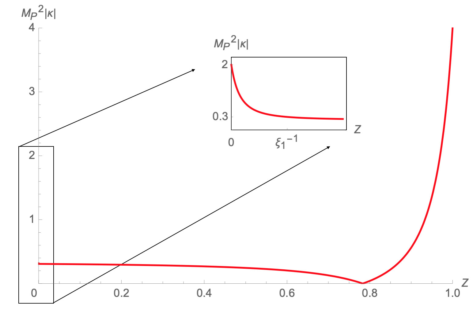
Figure 2: The absolute value of the field-manifold curvature $M_{P}^{2}|\kappa|$ for $\xi_{1}=10^{4}$ as a function of the inflaton field $Z$. We notice that its value for $Z\to 0$ is $M_{P}^{2}|\kappa|\sim 2$. For non-vanishing values of the field it rapidly decays and becomes approximately constant and equal to $M_{P}^{2}|\kappa|\sim 4/13$. Inflation takes place at field values $Z\sim\xi_{1}^{-1}$, meaning that the tensor-to-scalar ratio is expected to depend on the “equilibrated” value of the field-space curvature.

First, we analyze inflation. To this end, we leave out $\tilde{\rho}$ since it decouples from inflationary dynamics, the latter being for all practical purposes effectively single-field [18, 84, 36, 52]. For large $\xi_{1}$, the coefficient of the kinetic term of $\tilde{h}$ has the asymptotic form

$$\mathcal{K}_{\tilde{h}}\overset{\xi_{1}\rightarrow\infty}{\rightarrow}\frac{13}{2\tilde{h}^{2}}\;.$$ (5.40)

We are now in position to compare our findings with the action (5.4) of single-field metric Higgs inflation. Upon identifying $h$ with $\tilde{h}$, we see from eq. (5.39) that the potentials coincide and the coefficient of the kinetic terms only differ slightly in their numerical prefactors: the coefficient $6$ of metric Higgs inflation is replaced by $13/2$, as is evident from the asymptotic form (5.40). Correspondingly, the model (5.39) yields the inflationary indices 

$$n_{s}\approx 1-\frac{2}{N}\ ,~{}~{}~{}r\approx\frac{13}{N^{2}}\ .$$ (5.41)

We observe that the spectral index is identical to the one of metric Higgs inflation and the tensor-to-scalar ratio is slightly larger.

We checked the above findings with a full numerical analysis of the inflationary dynamics, where we use $U/\epsilon=5\cdot 10^{-7}$ for the CMB normalization [83] and choose $N=55$ as well as $\lambda=10^{-3}$ as typical values (see [67]). For comparison, we first analyze the original model (5.3), for which we obtain 

$$n_{s,\,\text{num}}^{\rm HI}=0.965\ ,~{}~{}~{}r_{\text{num}}^{\rm HI}=0.00351\ .$$ (5.42)

Repeating the same procedure in our model (5.39) (without performing any approximations in $\mathcal{K}_{\tilde{h}}$) yields

$$n_{s,\,\text{num}}=0.965\ ,~{}~{}~{}r_{\text{num}}=0.00379\ .$$ (5.43)

We see that the spectral indices coincide and the ratio $r_{\text{num}}/r_{\text{num}}^{\rm HI}=1.080$, which is very close to $13/12$. This confirms the validity of formula (5.41).

To study the geometry of field-space, we work with $Z=M_{P}^{2}/(\xi_{1}\tilde{h}^{2})$. Then we get from eq. (5.39)

$$S\approx\int\!\mathrm{d}^{4}x\sqrt{g}\left[\frac{M_{P}^{2}}{2}\mathring{R}-\frac{M_{P}^{2}}{2}\left(\gamma_{\rho\rho}(\partial_{\mu}\tilde{\rho})^{2}+\mathcal{K}_{Z}(\partial_{\mu}Z)^{2}\right)-\frac{\lambda M_{P}^{4}}{4\xi_{1}^{2}}\left(1-Z\right)^{2}\right]\ ,$$ (5.44)

where $\mathcal{K}_{Z}=(\frac{\mathrm{d}\tilde{h}}{\mathrm{d}Z})^{2}\mathcal{K}_{\tilde{h}}$. Now we can compute the field-space curvature (see eq. (4.28)) and the result is shown in fig. 2. We conclude that $M_{P}^{2}|\kappa|<4$ for all relevant field values. In particular, the limiting cases are $M_{P}^{2}\kappa=-2$ for $Z=0$ as well as $M_{P}^{2}\kappa=4$ for $Z=1$, corresponding to the limits of high energies and the electroweak epoch, respectively. In summary, we conclude that our model eq. (5.36) fulfills our conjecture. Conformality is preserved up to the Planck scale, i.e. $\Lambda_{\rm conf}\simeq M_{P}$, and in agreement with eq. (5.1), the predictions (5.41) are close to their counterparts (5.5) of single-field metric Higgs inflation.

Finally, we establish a direct connection of field-space curvature and inflationary predictions. For $\xi_{1}\gg 1$, our theory in the form (5.44) becomes

$$S\approx\int\!\mathrm{d}^{4}x\sqrt{g}\left[\frac{M_{P}^{2}}{2}\mathring{R}-\frac{M_{P}^{2}}{2}\left(4\xi_{1}^{5}Z(\partial_{\mu}\tilde{\rho})^{2}+\frac{13}{8}\frac{(\partial_{\mu}Z)^{2})}{Z^{2}}\right)-\frac{\lambda M_{P}^{4}}{4\xi_{1}^{2}}\left(1-Z^{2}\right)^{2}\right]\ ,$$ (5.45)

where we used that during inflation $\tilde{h}$ remains below $M_{P}$ and correspondingly $Z\gtrsim\mathcal{O}(1/\xi_{1})$. It is straightforward to compute the field-space curvature

$$M_{P}^{2}\kappa\approx-\frac{4}{13}\ .$$ (5.46)

Now we can use eq. (5.2), which is approximately valid for intervals of constant $\kappa$. Plugging in the value $-4/13$, we arrive at the tensor-to-scalar ratio $r=13/N^{2}$, in agreement with eq. (5.41). In summary, we conclude that both conformal properties and inflationary predictions can be deduced from the field-space curvature $\kappa$. In particular, an upper bound on $\kappa$ from the requirement of approximate conformal invariance leads to a lower bound on the tensor-to-scalar ratio.

Before turning to the conclusions, we shall evaluate the cutoff scale, above which perturbation theory breaks down. We can read it off from the potential as the energy scale that suppresses higher-dimensional operators. As is evident from eq. (5.39), we get

$$\Lambda_{\rm cutoff}\approx\frac{M_{P}}{\sqrt{\xi_{1}}}\;.$$ (5.47)

Taking into account effects of the non-canonical kinetic terms in eq. (5.39) does not lower the cutoff scale since the field-space curvature is bounded as $M_{P}^{2}|\kappa|\lesssim 1$ (see discussion in [87, 88]). We remark that the cutoff scale can depend on the background value of fields [89] and the result (5.47) only refers to vacuum. Moreover, we have only considered a biscalar theory; including other fields, in particular longitudinal gauge bosons, may also influence the cutoff scale [89, 90, 87, 88]. We leave an investigation of these points for future work.

6 Conclusions

In this paper, we first discussed in detail the constraints that linearly as well as nonlinearly realized conformal invariance imposes on the dynamics of multiscalar field theories. We showed that the target manifolds are endowed with a rather specific geometry. To reiterate our finding, there exists an appropriate set of variables in which the field-space metric of such conformal theories not only becomes block-diagonal (as is the case for theories invariant under dilatations only) but its uppermost left component—corresponding to the dilaton field “coordinate”—is unity. In other words, there always exists an appropriate set of variables such that the dilaton has a canonical kinetic term and no kinetic mixings with the rest of the fields. From the phenomenological point of view, the interesting situation corresponds to biscalar theories for which conformal symmetry fixes the target manifold to actually be flat.

We then presented how the inclusion of Einstein-Cartan gravity may be effectuated in a manner that preserves invariance under global dilatations. Deviating from the commonly used metric incarnation of General Relativity, one has to and actually should account for invariants constructed out of torsion, too. This has to be done with care as shown in our previous works [9, 1] (see also [67, 66, 91, 11]), where we devised a comprehensive set of criteria for constructing actions that encompass EC gravity and matter fields and propagate only the two polarizations of the massless graviton in their (purely) gravitational sector. In general, the presence of (large) nonminimal coupling(s) translates into gravitational contributions finding their way into the kinetic sector. This breaks conformal invariance at energies (significantly) below the Planck mass (whereas scale symmetry is preserved). We showed how to remedy the situation by formulating a condition ensuring approximate conformality of the resulting theories up to the Planck scale, where the theory becomes scale invariant “gravitationally.”

Our motivation for imposing this requirement is twofold. On the one hand, conformal invariance can improve the high-energy limit of the theory, by opening up a perspective for “self-completion” above the naive perturbative cutoff scale. On the other hand, subjecting a theory to such a condition reduces the built-in arbitrariness due to the numerous parameters that emerge in the EC formulation of GR. Investigating several concrete examples, we found indications that the situation may even be better than expected and – along with similar behavior noticed before  [36] – this led us to conjecture that the requirement of approximate conformality up to the Planck scale implies nearly model-independent statements about inflationary observables, which turn out to be close to the predictions of single-field metric Higgs inflation. How far this universality goes and if it holds in all parts of parameter space remains to be determined.

Appendix A Going beyond polynomial coefficient functions

In this appendix we shall briefly discuss what would happen if we deviated from the requirement of having the various coefficient functions polynomial in the fields $\phi_{1}$ & $\phi_{2}$. In other words, we will investigate what changes if the condition i) of our conjecture is dropped. To make things clear, we shall confine ourselves to an arguably extreme situation in which the curvature of the field-manifold is constant and equal to the Planck area for all field values. It will become clear that the inflationary predictions stop being unique, even though the curvature has been fixed and conformality of the kinetic sector is preserved until the Planck scale.

We start from (cf. eq. (4.28))

$$M_{P}^{2}\kappa=\frac{\gamma_{\rho\rho}^{\prime}\Gamma^{\prime}-2\Gamma\gamma_{\rho\rho}^{\prime\prime}}{2\Gamma^{2}}=1\ ,$$ (A.1)

with $\Gamma=\gamma_{\theta\theta}\gamma_{\rho\rho}-\gamma_{\rho\theta}^{2}$; assuming that $\gamma_{\rho\rho}\neq{\rm const.}$ we obtain [36]

$$\Gamma=-\frac{\gamma_{\rho\rho}^{\prime 2}}{2\gamma_{\rho\rho}-c}\ ,$$ (A.2)

where $c$ is an arbitrary (dimensionless) constant. Therefore, the inflaton’s kinetic function reads as (cf. eq. (5.14))

$$\mathcal{K}=\frac{\Gamma}{\gamma_{\rho\rho}}=-\frac{\gamma_{\rho\rho}^{\prime 2}}{\gamma_{\rho\rho}(2\gamma_{\rho\rho}-c)}\ .$$ (A.3)

Even though the arbitrariness has been reduced, we notice that the behavior of $\mathcal{K}$ is not unique but depends on whether or not one can neglect $c$. As long as inflation takes place for field values such that $\gamma_{\rho\rho}>c$, then the canonical field $\chi$ follows from an exponential map, $\chi\sim\ln\gamma_{\rho\rho}$, and the predictions mimic the ones of metric Higgs inflation. If, on the other hand, $\gamma_{\rho\rho}<c$, then the inflationary dynamics is more intricate and depend on $c$, too.

A particular choice of functions yielding this kind of behavior can for instance be the following “parity preserving” situation in eq. (4.3):

$$G_{aa}=\zeta^{a}_{\sigma}=\zeta^{a}_{\theta}=0\ .$$ (A.4)

Additionally, we take

$$G_{R}=\xi_{1}\cos^{2}\theta+\xi_{2}\sin^{2}\theta\ ,~{}~{}~{}f_{\theta\theta}=\frac{3}{2}\left(\frac{G_{R}^{\prime}}{G_{R}}\right)^{2}\frac{f(\theta)}{1+6G_{R}}\ ,$$ (A.5)

with $f(\theta)$ to be determined. From this choice, we obtain

$$\gamma_{\rho\rho}=6+\frac{1}{G_{R}}\ ,~{}~{}~{}\gamma_{\rho\theta}=3\frac{G_{R}^{\prime}}{G_{R}}\ ,~{}~{}~{}\gamma_{\theta\theta}=\frac{3}{2}\left(\frac{G_{R}^{\prime}}{G_{R}}\right)^{2}\left(1+\frac{f(\theta)}{1+6G_{R}}\right)\ ,$$ (A.6)

which translates into a rather involved $f(\theta)$

$$f(\theta)=-1-\frac{2}{3(2+(c+12)G_{R})}\ .$$ (A.7)

Clearly, the resulting $f_{\theta\theta}$ deviates from $f_{\theta\theta}=1$, which would be the only choice allowed according to our criteria i) - iii).

References

- [1] G. K. Karananas, M. Shaposhnikov, A. Shkerin, and S. Zell, “Scale and Weyl invariance in Einstein-Cartan gravity,” Phys. Rev. D 104 no. 12, (2021) 124014, arXiv:2108.05897 [hep-th].
- [2] É. Cartan, “Sur une généralisation de la notion de courbure de Riemann et les espaces à torsion,” Comptes Rendus, Ac. Sc. Paris 174 (1922) 593–595.
- [3] É. Cartan, “Sur les variétés à connexion affine et la théorie de la relativité généralisée (première partie),” in Annales scientifiques de l’École normale supérieure, vol. 40, pp. 325–412. 1923.
- [4] É. Cartan, “Sur les variétés à connexion affine, et la théorie de la relativité généralisée (première partie)(suite),” in Annales scientifiques de l’École Normale Supérieure, vol. 41, pp. 1–25. 1924.
- [5] É. Cartan, “Sur les variétés à connexion affine, et la théorie de la relativité généralisée (deuxième partie),” in Annales scientifiques de l’École normale supérieure, vol. 42, pp. 17–88. 1925.
- [6] A. Einstein, “Einheitliche Feldtheorie von Gravitation und Elektrizität,” Sitzungsber. Preuss. Akad. Wiss 22 (1925) 414.
- [7] A. Einstein, “Riemanngeometrie mit Aufrechterhaltung des Begriffes des Fern-Parallelismus,” Sitzungsber. Preuss. Akad. Wiss 17 (1928) 217.
- [8] A. Einstein, “Neue Möglichkeit für eine einheitliche Feldtheorie von Gravitation und Elektrizität,” Sitzungsber. Preuss. Akad. Wiss 18 (1928) 224.
- [9] G. K. Karananas, M. Shaposhnikov, A. Shkerin, and S. Zell, “Matter matters in Einstein-Cartan gravity,” Phys. Rev. D 104 no. 6, (2021) 064036, arXiv:2106.13811 [hep-th].
- [10] C. Rigouzzo and S. Zell, “Coupling metric-affine gravity to a Higgs-like scalar field,” Phys. Rev. D 106 no. 2, (2022) 024015, arXiv:2204.03003 [hep-th].
- [11] C. Rigouzzo and S. Zell, “Coupling Metric-Affine Gravity to the Standard Model and Dark Matter Fermions,” arXiv:2306.13134 [gr-qc].
- [12] C. Wetterich, “Cosmologies With Variable Newton’s ’Constant’,” Nucl. Phys. B 302 (1988) 645–667.
- [13] C. Wetterich, “Cosmology and the Fate of Dilatation Symmetry,” Nucl. Phys. B 302 (1988) 668–696, arXiv:1711.03844 [hep-th].
- [14] H. Dehnen and H. Frommert, “Higgs mechanism without Higgs particle,” Int. J. Theor. Phys. 32 (1993) 1135–1142.
- [15] C. Wetterich, “The Cosmon model for an asymptotically vanishing time dependent cosmological ’constant’,” Astron. Astrophys. 301 (1995) 321–328, arXiv:hep-th/9408025.
- [16] J. L. Cervantes-Cota and H. Dehnen, “Induced gravity inflation in the standard model of particle physics,” Nucl. Phys. B 442 (1995) 391–412, arXiv:astro-ph/9505069.
- [17] R. Foot, A. Kobakhidze, K. L. McDonald, and R. R. Volkas, “A Solution to the hierarchy problem from an almost decoupled hidden sector within a classically scale invariant theory,” Phys. Rev. D 77 (2008) 035006, arXiv:0709.2750 [hep-ph].
- [18] M. Shaposhnikov and D. Zenhausern, “Scale invariance, unimodular gravity and dark energy,” Phys. Lett. B 671 (2009) 187–192, arXiv:0809.3395 [hep-th].
- [19] M. Shaposhnikov and D. Zenhausern, “Quantum scale invariance, cosmological constant and hierarchy problem,” Phys. Lett. B 671 (2009) 162–166, arXiv:0809.3406 [hep-th].
- [20] M. E. Shaposhnikov and I. I. Tkachev, “Quantum scale invariance on the lattice,” Phys. Lett. B 675 (2009) 403–406, arXiv:0811.1967 [hep-th].
- [21] M. E. Shaposhnikov and F. V. Tkachov, “Quantum scale-invariant models as effective field theories,” arXiv:0905.4857 [hep-th].
- [22] J. Garcia-Bellido, J. Rubio, M. Shaposhnikov, and D. Zenhausern, “Higgs-Dilaton Cosmology: From the Early to the Late Universe,” Phys. Rev. D 84 (2011) 123504, arXiv:1107.2163 [hep-ph].
- [23] D. Blas, M. Shaposhnikov, and D. Zenhausern, “Scale-invariant alternatives to general relativity,” Phys. Rev. D 84 (2011) 044001, arXiv:1104.1392 [hep-th].
- [24] J. Garcia-Bellido, J. Rubio, and M. Shaposhnikov, “Higgs-Dilaton cosmology: Are there extra relativistic species?,” Phys. Lett. B 718 (2012) 507–511, arXiv:1209.2119 [hep-ph].
- [25] F. Bezrukov, G. K. Karananas, J. Rubio, and M. Shaposhnikov, “Higgs-Dilaton Cosmology: an effective field theory approach,” Phys. Rev. D 87 no. 9, (2013) 096001, arXiv:1212.4148 [hep-ph].
- [26] A. Monin and M. Shaposhnikov, “Spontaneously broken scale invariance and minimal fields of canonical dimensionality,” Phys. Rev. D 88 no. 6, (2013) 067701.
- [27] G. Marques Tavares, M. Schmaltz, and W. Skiba, “Higgs mass naturalness and scale invariance in the UV,” Phys. Rev. D 89 no. 1, (2014) 015009, arXiv:1308.0025 [hep-ph].
- [28] V. V. Khoze, “Inflation and Dark Matter in the Higgs Portal of Classically Scale Invariant Standard Model,” JHEP 11 (2013) 215, arXiv:1308.6338 [hep-ph].
- [29] C. Csaki, N. Kaloper, J. Serra, and J. Terning, “Inflation from Broken Scale Invariance,” Phys. Rev. Lett. 113 (2014) 161302, arXiv:1406.5192 [hep-th].
- [30] J. Rubio and M. Shaposhnikov, “Higgs-Dilaton cosmology: Universality versus criticality,” Phys. Rev. D 90 (2014) 027307, arXiv:1406.5182 [hep-ph].
- [31] D. M. Ghilencea, “Manifestly scale-invariant regularization and quantum effective operators,” Phys. Rev. D 93 no. 10, (2016) 105006, arXiv:1508.00595 [hep-ph].
- [32] A. Karam and K. Tamvakis, “Dark matter and neutrino masses from a scale-invariant multi-Higgs portal,” Phys. Rev. D 92 no. 7, (2015) 075010, arXiv:1508.03031 [hep-ph].
- [33] M. Trashorras, S. Nesseris, and J. Garcia-Bellido, “Cosmological Constraints on Higgs-Dilaton Inflation,” Phys. Rev. D 94 no. 6, (2016) 063511, arXiv:1604.06760 [astro-ph.CO].
- [34] G. K. Karananas and M. Shaposhnikov, “Scale invariant alternatives to general relativity. II. Dilaton properties,” Phys. Rev. D 93 no. 8, (2016) 084052, arXiv:1603.01274 [hep-th].
- [35] P. G. Ferreira, C. T. Hill, and G. G. Ross, “Scale-Independent Inflation and Hierarchy Generation,” Phys. Lett. B 763 (2016) 174–178, arXiv:1603.05983 [hep-th].
- [36] G. K. Karananas and J. Rubio, “On the geometrical interpretation of scale-invariant models of inflation,” Phys. Lett. B 761 (2016) 223–228, arXiv:1606.08848 [hep-ph].
- [37] A. Karam and K. Tamvakis, “Dark Matter from a Classically Scale-Invariant ,” Phys. Rev. D 94 no. 5, (2016) 055004, arXiv:1607.01001 [hep-ph].
- [38] P. G. Ferreira, C. T. Hill, and G. G. Ross, “Weyl Current, Scale-Invariant Inflation and Planck Scale Generation,” Phys. Rev. D 95 no. 4, (2017) 043507, arXiv:1610.09243 [hep-th].
- [39] P. G. Ferreira, C. T. Hill, and G. G. Ross, “No fifth force in a scale invariant universe,” Phys. Rev. D 95 no. 6, (2017) 064038, arXiv:1612.03157 [gr-qc].
- [40] D. M. Ghilencea, Z. Lalak, and P. Olszewski, “Standard Model with spontaneously broken quantum scale invariance,” Phys. Rev. D 96 no. 5, (2017) 055034, arXiv:1612.09120 [hep-ph].
- [41] A. Shkerin, “Electroweak vacuum stability in the Higgs-Dilaton theory,” JHEP 05 (2017) 155, arXiv:1701.02224 [hep-ph].
- [42] J. Rubio and C. Wetterich, “Emergent scale symmetry: Connecting inflation and dark energy,” Phys. Rev. D 96 no. 6, (2017) 063509, arXiv:1705.00552 [gr-qc].
- [43] A. Tokareva, “A minimal scale invariant axion solution to the strong CP-problem,” Eur. Phys. J. C 78 no. 5, (2018) 423, arXiv:1705.10836 [hep-ph].
- [44] S. Casas, M. Pauly, and J. Rubio, “Higgs-dilaton cosmology: An inflation–dark-energy connection and forecasts for future galaxy surveys,” Phys. Rev. D 97 no. 4, (2018) 043520, arXiv:1712.04956 [astro-ph.CO].
- [45] P. G. Ferreira, C. T. Hill, and G. G. Ross, “Inertial Spontaneous Symmetry Breaking and Quantum Scale Invariance,” Phys. Rev. D 98 no. 11, (2018) 116012, arXiv:1801.07676 [hep-th].
- [46] P. G. Ferreira, C. T. Hill, J. Noller, and G. G. Ross, “Inflation in a scale invariant universe,” Phys. Rev. D 97 no. 12, (2018) 123516, arXiv:1802.06069 [astro-ph.CO].
- [47] M. Shaposhnikov and A. Shkerin, “Gravity, Scale Invariance and the Hierarchy Problem,” JHEP 10 (2018) 024, arXiv:1804.06376 [hep-th].
- [48] C. Burrage, E. J. Copeland, P. Millington, and M. Spannowsky, “Fifth forces, Higgs portals and broken scale invariance,” JCAP 11 (2018) 036, arXiv:1804.07180 [hep-th].
- [49] Z. Lalak and P. Olszewski, “Vanishing trace anomaly in flat spacetime,” Phys. Rev. D 98 no. 8, (2018) 085001, arXiv:1807.09296 [hep-th].
- [50] D. Gorbunov and A. Tokareva, “Scalaron the healer: removing the strong-coupling in the Higgs- and Higgs-dilaton inflations,” Phys. Lett. B 788 (2019) 37–41, arXiv:1807.02392 [hep-ph].
- [51] D. Iosifidis and T. Koivisto, “Scale transformations in metric-affine geometry,” Universe 5 (2019) 82, arXiv:1810.12276 [gr-qc].
- [52] S. Casas, G. K. Karananas, M. Pauly, and J. Rubio, “Scale-invariant alternatives to general relativity. III. The inflation-dark energy connection,” Phys. Rev. D 99 no. 6, (2019) 063512, arXiv:1811.05984 [astro-ph.CO].
- [53] A. Shkerin, “Dilaton-assisted generation of the Fermi scale from the Planck scale,” Phys. Rev. D 99 no. 11, (2019) 115018, arXiv:1903.11317 [hep-th].
- [54] M. Herrero-Valea, I. Timiryasov, and A. Tokareva, “To Positivity and Beyond, where Higgs-Dilaton Inflation has never gone before,” JCAP 11 (2019) 042, arXiv:1905.08816 [hep-ph].
- [55] G. K. Karananas, V. Kazakov, and M. Shaposhnikov, “Spontaneous Conformal Symmetry Breaking in Fishnet CFT,” Phys. Lett. B 811 (2020) 135922, arXiv:1908.04302 [hep-th].
- [56] J. Rubio, “Scale symmetry, the Higgs and the Cosmos,” PoS CORFU2019 (2020) 074, arXiv:2004.00039 [gr-qc].
- [57] G. K. Karananas, M. Michel, and J. Rubio, “One residue to rule them all: Electroweak symmetry breaking, inflation and field-space geometry,” Phys. Lett. B 811 (2020) 135876, arXiv:2006.11290 [hep-th].
- [58] C. T. Hill and G. G. Ross, “Gravitational Contact Interactions and the Physical Equivalence of Weyl Transformations in Effective Field Theory,” Phys. Rev. D 102 (2020) 125014, arXiv:2009.14782 [gr-qc].
- [59] M. Piani and J. Rubio, “Higgs-Dilaton inflation in Einstein-Cartan gravity,” JCAP 05 no. 05, (2022) 009, arXiv:2202.04665 [gr-qc].
- [60] M. Shaposhnikov and A. Tokareva, “Anomaly-free scale symmetry and gravity,” Phys. Lett. B 840 (2023) 137898, arXiv:2201.09232 [hep-th].
- [61] M. Shaposhnikov and A. Tokareva, “Exact quantum conformal symmetry, its spontaneous breakdown, and gravitational Weyl anomaly,” Phys. Rev. D 107 no. 6, (2023) 065015, arXiv:2212.09770 [hep-th].
- [62] M. J. Duff, “Twenty years of the Weyl anomaly,” Class. Quant. Grav. 11 (1994) 1387–1404, arXiv:hep-th/9308075.
- [63] S. Rychkov, EPFL Lectures on Conformal Field Theory in D= 3 Dimensions. SpringerBriefs in Physics. 1, 2016. arXiv:1601.05000 [hep-th].
- [64] M. A. Luty, J. Polchinski, and R. Rattazzi, “The -theorem and the Asymptotics of 4D Quantum Field Theory,” JHEP 01 (2013) 152, arXiv:1204.5221 [hep-th].
- [65] M. Langvik, J.-M. Ojanperä, S. Raatikainen, and S. Rasanen, “Higgs inflation with the Holst and the Nieh–Yan term,” Phys. Rev. D 103 no. 8, (2021) 083514, arXiv:2007.12595 [astro-ph.CO].
- [66] M. Shaposhnikov, A. Shkerin, I. Timiryasov, and S. Zell, “Einstein-Cartan gravity, matter, and scale-invariant generalization ,” JHEP 10 (2020) 177, arXiv:2007.16158 [hep-th].
- [67] M. Shaposhnikov, A. Shkerin, I. Timiryasov, and S. Zell, “Higgs inflation in Einstein-Cartan gravity,” JCAP 02 (2021) 008, arXiv:2007.14978 [hep-ph]. [Erratum: JCAP 10, E01 (2021)].
- [68] F. L. Bezrukov and M. Shaposhnikov, “The Standard Model Higgs boson as the inflaton,” Phys. Lett. B 659 (2008) 703–706, arXiv:0710.3755 [hep-th].
- [69] Planck Collaboration, Y. Akrami et al., “Planck 2018 results. X. Constraints on inflation,” Astron. Astrophys. 641 (2020) A10, arXiv:1807.06211 [astro-ph.CO].
- [70] BICEP, Keck Collaboration, P. A. R. Ade et al., “Improved Constraints on Primordial Gravitational Waves using Planck, WMAP, and BICEP/Keck Observations through the 2018 Observing Season,” Phys. Rev. Lett. 127 no. 15, (2021) 151301, arXiv:2110.00483 [astro-ph.CO].
- [71] R. Jackiw and S. Y. Pi, “Tutorial on Scale and Conformal Symmetries in Diverse Dimensions,” J. Phys. A 44 (2011) 223001, arXiv:1101.4886 [math-ph].
- [72] K. Hinterbichler, Q. Liang, and M. Trodden, “EFT of conformal symmetry breaking,” Phys. Rev. D 107 no. 6, (2023) 065018, arXiv:2210.01139 [hep-th].
- [73] P. Di Francesco, P. Mathieu, and D. Senechal, Conformal Field Theory. Graduate Texts in Contemporary Physics. Springer-Verlag, New York, 1997.
- [74] A. Nicolis, R. Rattazzi, and E. Trincherini, “The Galileon as a local modification of gravity,” Phys. Rev. D 79 (2009) 064036, arXiv:0811.2197 [hep-th].
- [75] K. Hinterbichler, A. Joyce, and J. Khoury, “Non-linear Realizations of Conformal Symmetry and Effective Field Theory for the Pseudo-Conformal Universe,” JCAP 06 (2012) 043, arXiv:1202.6056 [hep-th].
- [76] G. Goon, K. Hinterbichler, A. Joyce, and M. Trodden, “Galileons as Wess-Zumino Terms,” JHEP 06 (2012) 004, arXiv:1203.3191 [hep-th].
- [77] S. M. Carroll, Spacetime and Geometry. Cambridge University Press, 7, 2019.
- [78] R. Zwicky, “The Dilaton Improves Goldstones,” arXiv:2306.12914 [hep-th].
- [79] L. Heisenberg, “A systematic approach to generalisations of General Relativity and their cosmological implications,” Phys. Rept. 796 (2019) 1–113, arXiv:1807.01725 [gr-qc].
- [80] J. Beltrán Jiménez, L. Heisenberg, and T. S. Koivisto, “The Geometrical Trinity of Gravity,” Universe 5 no. 7, (2019) 173, arXiv:1903.06830 [hep-th].
- [81] S. Cléry, H. M. Lee, and A. G. Menkara, “Higgs Inflation at the Pole,” arXiv:2306.07767 [hep-ph].
- [82] M. Shaposhnikov, A. Shkerin, and S. Zell, “Quantum Effects in Palatini Higgs Inflation,” JCAP 07 (2020) 064, arXiv:2002.07105 [hep-ph].
- [83] Planck Collaboration, Y. Akrami et al., “Planck 2018 results. X. Constraints on inflation,” Astron. Astrophys. 641 (2020) A10, arXiv:1807.06211 [astro-ph.CO].
- [84] J. Garcia-Bellido, J. Rubio, M. Shaposhnikov, and D. Zenhausern, “Higgs-Dilaton Cosmology: From the Early to the Late Universe,” Phys. Rev. D 84 (2011) 123504, arXiv:1107.2163 [hep-ph].
- [85] J. Martin, C. Ringeval, and V. Vennin, “Encyclopædia Inflationaris,” Phys. Dark Univ. 5-6 (2014) 75–235, arXiv:1303.3787 [astro-ph.CO].
- [86] J. Rubio, “Higgs inflation,” Front. Astron. Space Sci. 5 (2019) 50, arXiv:1807.02376 [hep-ph].
- [87] Y. Mikura and Y. Tada, “On UV-completion of Palatini-Higgs inflation,” JCAP 05 no. 05, (2022) 035, arXiv:2110.03925 [hep-ph].
- [88] G. K. Karananas, M. Shaposhnikov, and S. Zell, “Field redefinitions, perturbative unitarity and Higgs inflation,” JHEP 06 (2022) 132, arXiv:2203.09534 [hep-ph].
- [89] F. Bezrukov, A. Magnin, M. Shaposhnikov, and S. Sibiryakov, “Higgs inflation: consistency and generalisations,” JHEP 01 (2011) 016, arXiv:1008.5157 [hep-ph].
- [90] M. Shaposhnikov, A. Shkerin, and S. Zell, “Standard Model Meets Gravity: Electroweak Symmetry Breaking and Inflation,” Phys. Rev. D 103 no. 3, (2021) 033006, arXiv:2001.09088 [hep-th].
- [91] M. Shaposhnikov, A. Shkerin, I. Timiryasov, and S. Zell, “Einstein-Cartan Portal to Dark Matter,” Phys. Rev. Lett. 126 no. 16, (2021) 161301, arXiv:2008.11686 [hep-ph]. [Erratum: Phys.Rev.Lett. 127, 169901 (2021)].