Parton showering with higher-logarithmic accuracy for soft emissions

Abstract

The accuracy of parton-shower simulations is often a limiting factor in the interpretation of data from high-energy colliders. We present the first formulation of parton showers with accuracy one order beyond state-of-the-art next-to-leading logarithms, for classes of observable that are dominantly sensitive to low-energy (soft) emissions, specifically non-global observables and subjet multiplicities. This represents a major step towards general next-to-next-to-leading logarithmic accuracy for parton showers.

Parton showers simulate the repeated branching of quarks and gluons (partons) from a high momentum scale down to the non-perturbative scale of Quantum Chromodynamics (QCD). They are one of the core components of the general-purpose Monte Carlo event-simulation programs that are used in almost every experimental and phenomenological study involving high-energy particle colliders, such as CERN’s Large Hadron Collider (LHC). Parton-shower accuracy is critical at colliders, both because it limits the interpretation of data and because of the increasing importance of showers in training powerful machine-learning based data-analysis methods.

In the past few years it has become clear that it is instructive to relate the question of parton-shower accuracy to a shower’s ability to reproduce results from the field of resummation, which sums dominant (logarithmically enhanced) terms in perturbation theory to all orders in the strong coupling, $\alpha_{s}$. Given a logarithm $L$ of some large ratio of momentum scales, resummation accounts for terms $\alpha_{s}^{n}L^{n+1-p}$, N^pLL in a leading-logarithmic counting for $L\sim 1/\alpha_{s}$, or $\alpha_{s}^{n}L^{2n-p}$, N^pDL in a double-logarithmic counting, for $L\sim 1/\sqrt{\alpha_{s}}$.

Several groups have recently proposed parton showers designed to achieve next-to-leading logarithmic (NLL) and next-to-double logarithmic (NDL) accuracy for varying sets of observables [1, 2, 3, 4, 5, 6, 7, 8, 9, 10]. A core underlying requirement is the condition that a shower should accurately reproduce the tree-level matrix elements for configurations with any number of low-energy (“soft”) and/or collinear particles, as long as these particles are well separated in logarithmic phase space [11, 12, 2].

In this letter we shall demonstrate a first major step towards the next order in resummation in a full parton shower, concentrating on the sector of phase space involving soft partons. This sector is connected with two important aspects of LHC simulations, namely the total number of particles produced, and the presence of soft QCD radiation around leptons and photons (“isolation”), which is critical in their experimental identification in a wide range of LHC analyses. The corresponding areas of resummation theory, for subjet multiplicity [13, 14, 15] and so-called non-global logarithms [16, 17, 18, 19, 20, 21, 22, 23, 24, 25, 26, 27, 28, 29, 30, 31, 32, 33, 34, 35, 36, 37, 38, 39, 40, 41, 42], have seen extensive recent developments towards higher accuracy in their own right, with several groups working either on next-to-next-to-double logarithmic (NNDL) accuracy, $\alpha_{s}^{n}L^{2n-2}$, for multiplicity [43, 44] or next-to-single logarithmic (NSL) accuracy, $\alpha_{s}^{n}L^{n-1}$, for non-global logarithms [45, 46, 47, 48].

To achieve NSL/NNDL accuracy for soft-dominated observables, a crucial new ingredient is that the shower should obtain the correct matrix element even when there are pairs of soft particles that are commensurate in energy and in angle with respect to their emitter. Several groups have worked on incorporating higher-order soft/collinear matrix elements into parton showers [49, 50, 51, 52, 53, 54, 55, 56, 57, 58]. Our approach will be distinct in two respects: firstly, that it is in the context of a full shower that is already NLL accurate, which is crucial to ensure that the correctness of any higher-order matrix element is not broken by recoil effects from subsequent shower emissions; and secondly in that we will be able to demonstrate the logarithmic accuracy for concrete observables through comparisons to known resummations.

We will work in the context of the “PanGlobal” family of parton showers, concentrating on the final-state case [2]. As is common for parton showers, it organises particles into colour dipoles [59], a picture based on the limit of a large number of colours $N_{\text{{c}}}$. Such showers iterate $2\to 3$ splitting of colour dipoles, each splitting thus adding one particle to the ensemble, and typically breaking the original dipole into two dipoles. The splittings are performed sequentially in some ordering variable, $v$, for example in decreasing transverse momentum $k_{t}$. Given a dipole composed of particles with momenta $\tilde{p}_{i}$ and $\tilde{p}_{j}$, the basic kinematic map for producing a new particle $k$ is

$$\bar{p}_{k} =a_{k}\tilde{p}_{i}+b_{k}\tilde{p}_{j}+k_{\perp}\,,$$ (1a)

$$\bar{p}_{i} =(1-a_{k})\tilde{p}_{i}\,,$$ (1b)

$$\bar{p}_{j} =(1-b_{k})\tilde{p}_{j}\,.$$ (1c)

followed by a readjustment involving all particles so as to conserve momentum [60], §.1. For the original PanGlobal NLL shower, the splitting probability was given by

$$\frac{d\mathcal{P}_{n\to n+1}}{d\ln v}=\!\!\!\sum_{\{{\tilde{\imath}},{\tilde{\jmath}}\}\in\text{dip}}\int d\bar{\eta}\frac{d\phi}{2\pi}\frac{\alpha_{s}(k_{t})}{\pi}\left(1+\frac{\alpha_{s}(k_{t})K_{\textsc{cmw}}}{2\pi}\right)\\ \times\left[f(\bar{\eta})a_{k}P_{{\tilde{\imath}}\to ik}(a_{k})+f(-\bar{\eta})b_{k}P_{{\tilde{\jmath}}\to jk}(b_{k})\right]\,.$$ (2)

Here $P_{{\tilde{\imath}}\to ik}(a_{k})$ is a leading-order QCD splitting function, $\bar{\eta}=\frac{1}{2}\ln a_{k}/b_{k}+\text{const.}$, with the constant arranged so that $\bar{\eta}=0$ when the emission bisects the dipole in the event centre-of-mass frame, and $f(\bar{\eta})=1/(1+e^{-2\bar{\eta}})$ is a partitioning function. Additionally, the $\overline{\text{MS}}$ coupling, $\alpha_{s}(k_{t})$, uses at least 2-loop running, and $K_{\textsc{cmw}}=\left(67/18-\pi^{2}/6\right)C_{A}-5/9\,n_{f}$ [61].

Figure 1: Top: one shower history that produced a proximate $\{1,2\}$ soft pair. Bottom: other histories that could have led to the same configuration of momenta, also taken into account in correcting the branching. The dashed parton is emitted second in the showering history.

In moving towards higher accuracy, the two relevant elements are the analogues of the real and virtual corrections in a fixed-order calculation. We focus first on the real term, where we require the shower to generate the correct double-soft matrix element when two particles are produced at commensurate angles and (small) energies, while well-separated from all other particles.

Our approach is illustrated in Fig. 1. Consider the case where a dipole $ab$ first emits a soft gluon $\tilde{1}$, followed by a splitting of the dipole $\tilde{1}b$ whereby a new particle $2$ is emitted, and $\tilde{1}$ becomes $1$ after recoil. When the branching from Eq. (1) produces a particle $2$ from the $\tilde{1}b$ dipole, if $p_{1}.p_{2}<p_{2}.p_{b}$, we select the $\{1,2\}$ pair as the one whose double-soft effective matrix element needs correcting. To evaluate the double-soft correction to this configuration, we first identify all shower histories that could have produced the same nearby $\{1,2\}$ pair. This includes the history actually followed by the shower, as well as the case where $2$ was emitted from the $a\tilde{1}$ dipole, and two extra configurations where the shower produced a particle $\tilde{2}$ before $1$, i.e. where, in the second splitting, gluon $1$ was radiated with $2$ taking the recoil.

Each history $h$ is associated with an effective squared shower matrix element $|M_{\text{shower},h}|^{2}$, reflecting the probability that the shower, starting from the $ab$ system, would produce the $\{1,2\}$ pair in that order and colour configuration (we address the question of the flavour configuration below). $|M_{\text{shower},h}|^{2}$ is evaluated in the double-soft limit ([60], §.2.1). In principle, emission $2$ should be accepted with probability

$$P_{\text{accept}}=\frac{|M_{\text{{ds}}}|^{2}}{\sum_{h}|M_{\text{shower},h}|^{2}}.$$ (3)

where $|M_{\text{{ds}}}|^{2}$ is the known double-soft matrix element for emitting the $\{1,2\}$ soft pair from the $ab$ dipole [62, 63, 64]. In practice, however, there are regions where the shower underestimates the true matrix element, leading to $P_{\text{accept}}>1$. Nevertheless, we find that $P_{\text{accept}}$ always remains smaller than some finite value $\Omega$. We therefore enhance the splitting probability Eq. (2) by an overhead factor $\Omega$, and accept the emission with probability $P_{\text{accept}}/\Omega$.

The numerator and denominator in Eq. (3) are evaluated in the same double-soft limit, defined by rescaling $p_{1}\rightarrow\lambda p_{1}$, $p_{2}\rightarrow\lambda p_{2}$ and taking the limit $\lambda\rightarrow 0$. This ensures that $P_{\text{accept}}=1$ when $1$ and $2$ are well separated, thus not affecting regions where the shower was already correct.

The acceptance procedure is sufficient to ensure the proper generation of the $\{1,2\}$ kinematics, but not the relative weights of the $a12b$ and $a21b$ colour connections, which is crucial to reproduce the pattern of subsequent much softer radiation from the $\{a,1,2,b\}$ system, as required for NSL accuracy. To address this problem, we evaluate $F_{\text{shower}}^{(12)}$, the fraction of the shower effective double-soft matrix element associated with the $a12b$ colour connection, and similarly $F_{\text{{ds}}}^{(12)}$ for the full double-soft matrix element, in its large-$N_{\text{{c}}}$ limit [63, 64]. If the shower has generated the $a12b$ colour connection and $F_{\text{shower}}^{(12)}>F_{\text{{ds}}}^{(12)}$, then we swap the colour connection with probability

$$P_{\text{swap}}=\frac{F_{\text{shower}}^{(12)}-F_{\text{{ds}}}^{(12)}}{F_{\text{shower}}^{(12)}}.$$ (4)

We apply a similar procedure when the shower generates the $a21b$ connection. In practice, we precede the colour swap with an analogous procedure for adjusting the relative weights of $gg$ and $q\bar{q}$ flavours for the $\{1,2\}$ pair. An alternative would have been to apply $P_{\text{accept}}$ separately for each colour ordering and flavour combination, however when we investigated that option for the PanGlobal class of showers, we encountered regions of phase space where the acceptance probability was unbounded. Illustrative plots of the shower matrix element and corrections are given in the supplemental material [60], §.2.2.

Next, we address the question of virtual corrections. When $\tilde{1}$ is produced in the deep soft-collinear region of the $ab$ dipole, i.e. $\theta_{a\tilde{1}}\ll\theta_{ab}$ or $\theta_{\tilde{1}b}\ll\theta_{ab}$, the inclusion of $K_{\textsc{cmw}}$ in Eq. (2) already accounts for second order contributions to the branching probability in the soft-collinear region, as required for NLL accuracy for global event shapes. However, in general, $K_{\textsc{cmw}}$ alone is not sufficient when $\theta_{a1}\sim\theta_{1b}\sim\theta_{ab}$, notably because of the non-trivial $\bar{\eta}$ dependence in Eq. (2) and the way in which it connects with the overall event momentum $Q$. Therefore we need to generalise $K_{\textsc{cmw}}\to K(\Phi_{\tilde{1},ab})$, where the full $K$ is a function of the kinematics of $\tilde{1}$ and of the opening angle of the $ab$ dipole. In the same vein as the MC@NLO [65] and POWHEG [66, 67] methods and their MINLO [68, 69] extension, the correct next-to-leading-order (NLO) normalisation for the emission is given by

$$K(\Phi_{\tilde{1},ab})=V(\Phi_{\tilde{1},ab})+\int d\Phi^{\text{{ps}}}_{12/\tilde{1}}|M^{\text{{(ps)}}}_{12/\tilde{1}}|^{2}-\Delta^{(\text{{ps}},1)}_{\tilde{1}}.$$ (5)

Here, $V$ is the exact QCD 1-loop contribution for a single soft emission, renormalised at scale $\mu=k_{t,\tilde{1}}$; $d\Phi^{\text{{ps}}}_{12/\tilde{1}}|M^{\text{{(ps)}}}_{12/\tilde{1}}|^{2}$ is the product of shower phase space and matrix element associated with real $\tilde{1}\to 12$ branching, including double-soft corrections; and $\Delta^{(\text{{ps}},1)}_{\tilde{1}}$ is the coefficient of $\alpha_{s}/(2\pi)$ in the fixed-order expansion of the shower Sudakov factor. To aid in the evaluation of $K(\Phi_{\tilde{1},ab})$ we make use of two main elements: firstly, in the soft-collinear limit, $K(\Phi_{\tilde{1},ab})\to K_{\textsc{cmw}}$; secondly, both $V(\Phi_{\tilde{1},ab})$ and $\Delta^{(\text{{ps}},1)}_{\tilde{1}}$ are independent of the rapidity of $\tilde{1}$, as long as $\tilde{1}$ is soft and (for $\Delta^{(\text{{ps}},1)}_{\tilde{1}}$) kept at some fixed value of the evolution scale. We can therefore reformulate Eq. (5) as $K=K_{\textsc{cmw}}+\Delta K$, with

$$\Delta K=\int_{r}d\Phi^{\text{{(ps)}}}_{12/\tilde{1}}\,|M^{\text{{(ps)}}}_{12/\tilde{1}}|^{2}-\int_{r_{\text{sc}}}d\Phi^{\text{{(ps)}}}_{12/\tilde{1}_{\text{sc}}}|M^{\text{{(ps)}}}_{12/\tilde{1}_{\text{sc}}}|^{2}.$$ (6)

In the second term, $\tilde{1}_{\text{sc}}$ is at the same shower scale $v$ as $\tilde{1}$, but shifted by a constant in rapidity with respect to $ab$ so as to be in the soft-collinear region, wherein $K(\Phi_{{\tilde{1}}_{\text{sc}},ab})\rightarrow K_{\textsc{cmw}}$. The labels $r$ and $r_{\text{sc}}$ indicate a regularisation of the phase space, which should be equivalent between the two terms. Specifically, we separate $M_{\text{DS}}$ in Eq. (3) into correlated and uncorrelated parts, respectively those involving $C_{F}C_{A}$ versus $C_{F}^{2}$ colour factors for the $\bar{q}ggq$ matrix element. For the correlated part, we cut on the relative transverse momentum of $1$ and $2$, while for the uncorrelated part, we cut on the transverse momentum with respect to the $ab$ dipole and impose $|\Delta y_{12}|<\Delta y_{\max}$. In practice we tabulate $\Delta K$ as a function of $\theta_{ab}$, $\bar{\eta}_{\tilde{1}}$, and $\phi_{\tilde{1}}$, though one could also envisage on-the-fly evaluation. We incorporate $\Delta K$ in Eq. (2), through a multiplicative factor $1+\tanh[\frac{\alpha_{s}}{2\pi}\,\Delta K(1-a_{k})(1-b_{k})]$. This form keeps the correction positive and bounded. It also leaves the shower unmodified in the hard-collinear region.

We study the above approach with several variants of the PanGlobal shower. All have been adapted relative to Ref. [2] with regards to the precise way in which they restore momentum conservation after the map of Eq. (1). This was motivated by the discovery that in higher-order shower configurations involving three similarly collinear hard particles, the original recoil prescription could lead to unwanted long-distance kinematic side effects. Details are given in the supplemental material [60], §.1, and tests were carried out using the method of Ref. [70].

We will consider three variants of the PanGlobal shower: two choices of the ordering variable, $\sim k_{t}\theta^{\beta}$ with $\beta=0$ (PG_β=0) and $1/2$ (PG_β=1/2), and also a “split-dipole-frame” $\beta=0$ variant (PG${}^{\text{sdf}}_{\beta=0}$), which replaces $f(\pm\bar{\eta})\to f(\pm\eta)$ in Eq. (2), with $\eta=\frac{1}{2}\log a_{k}/b_{k}$. The $\eta=0$ transition region bisects the dipole in its rest frame rather than the event frame. This makes the $\tilde{1}\to 12$ branching independent of the $\tilde{1}$ rapidity in the dipole frame, resulting in $\Delta K=0$. Illustrative plots of $\Delta K$ and its impact are given in Ref. [60], §.2.3. For the three shower variants, the overhead factors $\Omega$ associated with Eq. (3) are respectively taken equal to $3.1$, $20$ and $4$, independently of the dipole kinematics.

All results, both with and without double-soft corrections, include NLO $2$-jet matching [71], which is required for the NNDL/NSL accuracy that we aim for. Spin correlations [72, 73] are turned off, because we have yet to integrate them with the double-soft corrections. The double-soft corrections are implemented at large-$N_{\text{{c}}}$, in such a way as to preserve the full-$N_{\text{{c}}}$ NLL/NDL accuracies obtained in Ref. [74] for global observables and multiplicities. All events have (positive) unit weight.

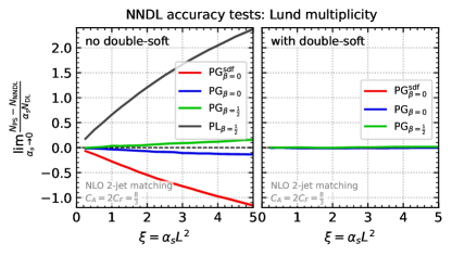
Figure 2: The result of Eq. (7) for three variants of the PanGlobal shower without double-soft corrections (left) and with them (right). The latter are consistent with NNDL accuracy. The bands represent statistical errors in an $\alpha_{s}\to 0$ extrapolation based on four finite $\alpha_{s}$ values.

To test the enhanced logarithmic accuracy of the shower, the first observable that we consider is the Lund subjet multiplicity [43] in $e^{+}e^{-}\to q\bar{q}$ events. This is a perturbatively calculable observable that is conceptually close to the experimentally important total charged-particle multiplicity. For a centre-of-mass energy $Q$ and a transverse momentum cutoff $k_{t}$, the subjet multiplicity has a double-logarithmic resummation structure $\alpha_{s}^{n}L^{2n}$ with $L=\ln k_{t}/Q$. The PanGlobal showers already reproduce terms up to NDL $\alpha_{s}^{n}L^{2n-1}$. The addition of the double-soft corrections and matching [71] is expected to bring NNDL accuracy, $\alpha_{s}^{n}L^{2n-2}$. To test this, in Fig. 2, we examine

$$\lim_{\alpha_{s}\to 0}\left.\frac{N_{\text{{ps}}}-N_{\text{{nndl}}}}{\alpha_{s}N_{\text{{dl}}}}\right|_{\text{fixed {\hbox{}}\alpha_s{\hbox{ L^2}}}},$$ (7)

where $N_{\text{{ps}}}$ is the parton-shower result and $N_{\text{{nndl}}}$ ($N_{\text{{dl}}}$) is the known analytic NNDL (DL) result [43]. The $\alpha_{s}\to 0$ limit follows the procedure from earlier work [2]. Eq. (7) is expected to be zero if the parton shower is NNDL accurate. The original showers, without double-soft corrections (left), clearly differ from each other and from zero, by up to $\sim 100\%$. With double-soft corrections turned on (right), all three PanGlobal variants are consistent with zero, i.e. with NNDL accuracy, to within $\sim 1\%$.

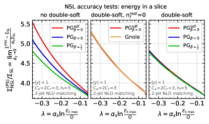
Figure 3: Determinations of $\Sigma_{\text{{nsl}}}^{(\text{{ps}})}/\Sigma_{\text{{sl}}}$ for the transverse energy in a slice. Left: parton showers without double-soft corrections illustrating NSL differences between them. Middle: with double-soft corrections but $n_{f}^{\text{real}}\!=0$ (cf. text for details), for comparison with the Gnole NSL code. Right: with full double-soft corrections, showing NSL agreement between the three PanGlobal showers.

Next we turn to the study of non-global logarithms at leading colour. These were recently calculated at NSL accuracy [45, 46, 48], $\alpha_{s}^{n}L^{n-1}$, and are available in the corresponding “Gnole” code [46]. We again consider $e^{+}e^{-}$ events, and sum the transverse energies ($E_{t}$) of particles with $|y|<1$, where $y$ is the rapidity with respect to an axis determined by clustering the event to two jets with the Cambridge algorithm [75]. The fraction of events where the sum is below some $E_{t,\max}$ is denoted by $\Sigma$ and for a given shower we define

$$\Sigma_{\text{{nsl}}}^{(\text{{ps}})}=\lim_{\alpha_{s}\to 0}\left.\frac{\Sigma^{(\text{{ps}})}-\Sigma_{\text{{sl}}}}{\alpha_{s}}\right|_{\text{fixed {\hbox{}}\alpha_s{\hbox{ L}}}},\hskip 28.00006pt\quad L\equiv\ln\frac{E_{t,\max}}{Q}.$$ (8)

Fig. 3 (left) shows $\Sigma_{\text{{nsl}}}^{(\text{{ps}})}/\Sigma_{\text{{sl}}}$ for our three PanGlobal variants without double-soft corrections. As expected, they differ.

Fig. 3 (middle) compares our PG${}_{\beta=0}^{\text{sdf}}$ shower with double-soft corrections to the NSL Gnole code, showing good agreement, within $<1\%$. Gnole has $n_{f}=0$ in the real contribution and counterterm, but keeps the full $n_{f}=5$ in the running of the coupling and inclusive $K_{\textsc{cmw}}$ (“$n_{f}^{\text{real}}=0$”). Among our showers it is relatively straightforward to make the same choice with PG${}_{\beta=0}^{\text{sdf}}$, in particular because $\Delta K=0$. Also, Gnole uses the thrust axis, while we use the jet axis; this is beyond NSL as the two axes coincide for hard three-parton events.

Fig. 3 (right) shows the results from our three PanGlobal showers with complete (full-$n_{f}$) double-soft corrections included. They agree with each other to within 1% of the NSL contribution, providing a powerful test of the consistency of the full combination of the double-soft matrix element and $\Delta K$ across the variants. That plot also provides the first NSL calculation of non-global logarithms to include the full $n_{f}$ dependence. An extended selection of results and comparisons is provided in §.3 of Ref. [60].

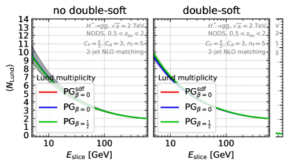
Figure 4: Distribution of energy in a slice $|y|<0.5$ for the PanGlobal shower without double-soft corrections (left) and with them (right). The bands represent renormalisation scale variation, with NLO scale-compensation enabled only for the results with double-soft corrections.

We close with a brief examination of the phenomenological implications of the advances presented here. We consider $e^{+}e^{-}\to Z^{*}\to\text{jets}$ at $Q=2\,\mathrm{TeV}$. This choice is intended to help gauge the size of non-global effects at the energies being probed today at the LHC. Fig. 4 shows results for the distribution of energy flow in a rapidity slice, defined with respect to the 2-jet axis, without double-soft corrections (left) and with them, i.e. at NSL accuracy (right). It uses the nested ordered double-soft (NODS) colour scheme, which while not full-$N_{\text{{c}}}$ accurate for non-global logarithms, numerically coincides with the full-$N_{\text{{c}}}$ single logarithmic results of Refs. [40, 39, 38], to within their percent-level numerical accuracy [74]. With a central scale choice (solid lines), the impact of the NSL corrections is modest. This is consistent with the observation from Fig. 3 that the NLL PanGlobal showers are numerically not so far from NSL accurate. However, the NSL double-soft corrections do bring a substantial reduction in the renormalisation scale uncertainty, from about $10\%$ to just a few percent. Conclusions are similar for $H^{*}\to gg$.

The results here provide the first demonstration that it is possible to augment parton-shower accuracy beyond NDL/NLL. Specifically, our inclusion of real and virtual double-soft effects has simultaneously brought NNDL/NSL accuracy for two phenomenologically important classes of observable: multiplicities, and energy flows as relevant for isolation. It has also enabled the first leading-colour, full-$n_{f}$ predictions for NSL non-global logarithms. Overall, our methods and results represent a significant step towards a broader future goal of general next-to-next-to-leading logarithmic accuracy in parton showers.

Supplemental material

.1 Event-wide momentum conservation for the PanGlobal shower

Compared to the original formulation in Ref. [2], this study introduces a revised rescaling procedure for the kinematic map of the PanGlobal parton shower. Here we outline an important flaw identified in the original PanGlobal map, before detailing two amended versions which rectify it, one of which has been used for all results in this article.

.1.1 Unsafety of the original formulation

Given a set of splitting variables $\{v,\bar{\eta},\phi\}$ generated according to Eq. (2), the original PanGlobal kinematic map of Ref. [2] proceeds by first constructing a set of intermediate post-branching momenta according to Eq. (1), conserving only longitudinal momentum within the emitting dipole system. All momenta in the event are subsequently rescaled by a factor $r=\sqrt{Q^{2}/(Q+k_{\perp})^{2}}$, which serves to bring the total invariant mass of the event back to $Q^{2}$. Finally, a Lorentz boost is applied to all particles restoring the total four-momentum in the event, from $r(Q+k_{\perp})$ to $Q$.

In all kinematic limits where shower emissions are well-separated in logarithmic phase-space, i.e. all limits pertaining to NLL accuracy, the rescaling factor, $r$, tends to one. While investigating kinematic configurations relevant beyond NLL accuracy, we found a specific sequence of emissions, involving three similarly-collinear hard particles, that leads to $r$ differing from one by an $\mathcal{O}(1)$ amount.

The fact that a double-unresolved configuration produces long-range (event-wide) $\mathcal{O}(1)$ momentum shifts is in contradiction with the fundamental construction principle of the PanScales showers. This spurious effect evades NLL-accuracy tests, which are by definition insensitive to triple-collinear corrections. Nevertheless, since configurations with three similarly-collinear hard particles can be generated at arbitrarily small angles, the resulting large rescalings technically mean that the original PanGlobal rescaling prescription violates infrared-and-collinear safety.

The origin of large rescaling coefficients can be simply illustrated as follows. Consider the situation where, in the event frame, one has a highly-energetic dipole ${\tilde{\imath}}{\tilde{\jmath}}$, with $E_{\tilde{\imath}}\sim Q$, $E_{\tilde{\jmath}}\sim Q$, and an opening angle $\theta_{{\tilde{\imath}}{\tilde{\jmath}}}\ll 1$. We then radiate a hard-collinear emission $k$ from the ${\tilde{\imath}}{\tilde{\jmath}}$ dipole using the kinematic map of Eq. (1). The transverse momentum of the emission (with respect to the dipole) is given by $k_{t}^{2}=a_{k}b_{k}m_{{\tilde{\imath}}{\tilde{\jmath}}}^{2}$ which, in the commensurate triple-collinear limit ($a_{k}\sim b_{k}\sim 1$), becomes $k_{t}^{2}\sim m_{{\tilde{\imath}}{\tilde{\jmath}}}^{2}\sim\theta_{{\tilde{\imath}}{\tilde{\jmath}}}^{2}Q^{2}$. Consequently, in the ${\tilde{\imath}}{\tilde{\jmath}}$ dipole rest frame, the original dipole momenta and the transverse contribution are all commensurate, and of order $\theta_{{\tilde{\imath}}{\tilde{\jmath}}}Q$. Boosting to the event frame, all momenta receive a large Lorentz boost factor $\gamma\sim(E_{\tilde{\imath}}+E_{\tilde{\jmath}})/m_{{\tilde{\imath}}{\tilde{\jmath}}}\sim 1/\theta_{{\tilde{\imath}}{\tilde{\jmath}}}$. In particular, this results in the transverse component having an energy of order $Q$ in the event frame, or equivalently $k_{\perp}.Q\sim(1/\theta_{{\tilde{\imath}}{\tilde{\jmath}}})(\theta_{{\tilde{\imath}}{\tilde{\jmath}}}Q).Q\sim Q^{2}$. Since transverse components are not conserved by the map of Eq. (1), one obtains a rescaling factor $r$ that significantly departs from one.

Below, we introduce two small adaptations of the original kinematic rescaling that each cure this issue.

.1.2 Updated prescriptions with local rescaling

The essential idea of the updated prescriptions that we introduce below is to avoid spuriously large rescalings of the event as a whole by absorbing the potentially large energy component of the transverse momentum $k_{\perp}$ via a dipole-local rescaling. We start with the PanGlobal momentum map from Eq. (1).

In the first of our two updated prescriptions, instead of applying a global rescaling to all the momenta in the event, we rescale $\bar{p}_{i}$, $\bar{p}_{j}$ and $\bar{p}_{k}$ by a local rescaling factor $r_{\scriptscriptstyle{\text{L}}}$. As with the original variant, we fix the rescaling by imposing that the invariant mass of the event is returned to $Q^{2}$. Defining time-like four-momenta $\bar{p}_{ijk}=\bar{p}_{i}+\bar{p}_{j}+\bar{p}_{k}$ and $\tilde{p}_{m}=Q-\tilde{p}_{i}-\tilde{p}_{j}$, we find

$$r_{\scriptscriptstyle{\text{L}}}=\frac{-\tilde{p}_{m}.\bar{p}_{ijk}+\sqrt{(\tilde{p}_{m}.\bar{p}_{ijk})^{2}+\bar{p}_{ijk}^{2}\,(Q^{2}-\tilde{p}_{m}^{2})}}{\bar{p}_{ijk}^{2}}.$$ (9)

After the (local) rescaling the whole event undergoes a Lorentz boost so as to restore the total four-momentum of the event to its original value $Q$ (as in the original PanGlobal prescription). This is the prescription used throughout this paper.

A second possibility is as follows. Noting that the origin of the issue with global rescaling lies in the large energy component of $k_{\perp}$, one can proceed with a hybrid approach whereby one first applies a local rescaling $r_{\scriptscriptstyle{\text{L}}}^{\prime}$ to restore the dipole energy in the original event frame, i.e. imposing $r_{\scriptscriptstyle{\text{L}}}^{\prime}\,\bar{p}_{ijk}.Q=(\tilde{p}_{i}+\tilde{p}_{j}).Q$. One subsequently applies a global rescaling $r_{\scriptscriptstyle{\text{G}}}^{\prime}$ to restore the invariant mass $Q^{2}$ of the whole event, followed by a Lorentz boost, as in the original formulation. We find

$$r_{\scriptscriptstyle{\text{L}}}^{\prime}=\frac{(\tilde{p}_{i}+\tilde{p}_{j}).Q}{\bar{p}_{ijk}.Q},\qquad\text{ and }\qquad r_{\scriptscriptstyle{\text{G}}}^{\prime}=\sqrt{\frac{Q^{2}}{(\tilde{p}_{m}+r_{\scriptscriptstyle{\text{L}}}^{\prime}\bar{p}_{ijk})^{2}}}.$$ (10)

Note that similar rescaling strategies can be adopted in the formulation of the PanGlobal shower for $pp$ collisions, deep-inelastic scattering and vector-boson fusion (see Ref. [10] for details).

The specific choice between the two updated schemes does not affect the tests carried out in this paper. This owes to the following two facts: firstly, in the double-soft region all rescalings go to one (both in the original formulation and in the two amended versions introduced here); secondly, for the special case of the first emission, where there are only three post-branching momenta, all three maps are identical, meaning that the matching procedure is also unaffected [71].

To validate the new rescaling prescription, we have performed numerical tests similar to the infrared-and-collinear-safety tests carried out for flavoured-jet algorithms in Ref. [70]. While the original prescription fails these tests, the new approaches described here pass them. Additionally, we have extended those tests to automate the verification of the more stringent PanScales criteria, proceeding as follows. First, we generate an initial set of emissions. Second, we add new emissions widely separated from the initial ones by at least a distance $\Delta$ in a logarithmic phase-space (equivalently, the Lund plane). We then check that the recoil induced on the initial emissions decays exponentially with increasing $\Delta$. While the original global rescaling approach fails these tests (as do standard dipole showers), the new variants pass. Note that if we further impose that the additional emissions are themselves widely separated in logarithmic phase-space, both the original and new rescaling prescriptions pass the test, in accordance with the expectations from the NLL matrix-element tests performed in earlier work.

.2 Matrix element tests and $\Delta K$

This section records expressions for the effective shower matrix elements, before giving illustrative results regarding the validation of the two key elements of our double-soft corrections, namely the real matrix-element corrections and the virtual $\Delta K$ correction.

.2.1 Effective shower matrix elements

The total effective squared shower matrix element in Eq. (3), at large-$N_{\text{{c}}}$, describing the radiation of a double-soft gluon or quark pair, $\left\{1,2\right\}$, from a dipole $ab$, is most conveniently expressed as a sum of contributions associated to the two contributing colour connections, $a12b$ and $a21b$ :

$$\sum_{h}\,|M_{\mathrm{shower},h}|^{2}=\sum_{h\in a12b}|M_{\mathrm{shower},h}^{(12)}|^{2}+\sum_{h\in a21b}|M_{\mathrm{shower},h}^{(21)}|^{2}.$$ (11)

The contribution associated to the $a21b$ colour ordering has the form

$$\sum_{h\in a21b}|M_{\mathrm{shower},h}^{(21)}|^{2}= (8\pi\alpha_{s})^{2}\,2C_{1}\,\mathcal{J}\left[f(\hat{\eta}_{2})\,2C_{2}\,\delta_{a\rightarrow a2}+f(-\hat{\eta}_{2})\,z_{2}\,P_{\tilde{1}\rightarrow 12}(z_{2})\right]\Theta(v_{\tilde{1}}>v_{2})\,+\,\{1\leftrightarrow 2\}\,,$$ (12)

wherein $\mathcal{J}$, $\bar{\eta}_{2}$, and $z_{2}$ are given in terms of invariants $s_{ij}=2p_{i}.p_{j}$ and $s_{i}=2p_{i}.Q$ as follows

$$\mathcal{J}= \frac{s_{ab}}{s_{b1}(s_{a1}+s_{a2})}\frac{s_{a1}}{s_{a2}s_{12}}, \bar{\eta}_{2}= \frac{1}{2}\log\left(\frac{s_{a}s_{12}}{s_{1}s_{a2}}\right)=\eta_{2}+\frac{1}{2}\log\left(\frac{s_{a}s_{a1}}{s_{1}(s_{a1}+s_{a2})}\right), z_{2}= \frac{s_{a2}}{s_{a1}+s_{a2}}.$$ (13)

The angular dipole partitioning functions, $f(\pm\bar{\eta}_{2})$, and the splitting functions, $P_{\tilde{1}\rightarrow 12}(z_{2})$, are as given in Ref. [2]; for PG_β=0 and PG_β=1/2 we have $\hat{\eta}_{2}=\bar{\eta}_{2}$, as in Eq. (2), while for PG${}^{\text{sdf}}_{\beta=0}$ this is modified to $\hat{\eta}_{2}=\eta_{2}$. The $\delta_{a\rightarrow a2}$ factor is equal to one when the radiated pair comprises of gluons, and zero when it consists of quarks. Colour factors $C_{1}$ and $C_{2}$ are both equal to $C_{F}$, with $C_{A}=2C_{F}$ in the large-$N_{\text{{c}}}$ limit.

The final theta function in Eq. (12) reflects the ordering of the emissions with respect to the shower evolution variable $v$. The evolution variable was defined in terms of $k_{t}$ and $\bar{\eta}$ in Ref. [2] through $k_{t}=\rho ve^{\beta|\bar{\eta}|}$. $\Theta(v_{\tilde{1}}>v_{2})$ in Eq. (12) is then fully specified given Eq. (13) for $\bar{\eta}_{2}$ together with the following additional components

$$k_{t,\tilde{1}}^{2} =\frac{s_{b1}(s_{a1}+s_{a2})^{2}}{s_{ab}s_{a1}}, \rho_{\tilde{1}} =\left(\frac{s_{a}s_{b}}{Q^{2}s_{ab}}\right)^{\frac{\beta}{2}}, \bar{\eta}_{\tilde{1}} =\frac{1}{2}\log\left(\frac{s_{a}s_{b1}}{s_{b}s_{a1}}\right), k_{t,2}^{2} =\frac{s_{a2}s_{12}}{s_{a1}}, \rho_{2} =\left(\frac{s_{a}s_{1}}{Q^{2}s_{a1}}\right)^{\frac{\beta}{2}}.$$ (14)

Finally, the contribution to the total effective squared shower matrix element arising from the $a12b$ colour ordering, $\sum_{h\in a12b}\,|M_{\mathrm{shower},h}^{(12)}|^{2}$, is given by swapping $a\leftrightarrow b$ everywhere on the right-hand side of Eq. (12).

.2.2 Real double-soft matrix-element corrections

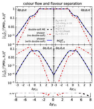
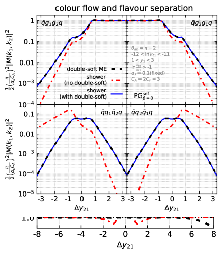
Figure 5: Left: rate of emission before (dashed-dot red) and after (solid blue) double-soft matrix-element corrections at $\mathcal{O}(\alpha_{s}^{2})$. Right: decomposition in terms of colour flows and flavour channels.

In Fig. 5 (left) we provide an illustration of one of the matrix element tests that we have carried out. It is shown for the PG${}^{\text{sdf}}_{\beta=0}$ shower. We start with a dipole $ab$ with an opening angle of $\theta_{ab}=\pi-2$ in the event centre-of-mass frame. From that system, we generate two soft emissions, and select those configurations where the higher-$k_{t}$ emission ($1$) is in a window $-12<\ln k_{t1}/Q<-11$ and $1<y_{1}<3$, while the lower-$k_{t}$ emission ($2$) satisfies $\ln k_{t2}/k_{t1}>-1$. We determine transverse momenta and rapidities in the dipole centre-of-mass frame and, for the purpose of Fig. 5, restrict our attention to configurations for which, in that frame, the two emissions are both in the $ab$ dipole’s primary Lund plane [12]. The upper panel shows the differential distribution of the rapidity difference between the two emissions, $\Delta y_{21}=y_{2}-y_{1}$.

The results in Fig. 5 have been normalised to $2\,\!(\alpha_{s}C_{A}/\pi)^{2}$ which is the expected result for large $\Delta y_{21}$, at large-$N_{\text{{c}}}$, as long as particle $2$ is still soft. The red (dot-dashed) curve shows the default shower, without any double-soft correction, while the black curve shows the actual double-soft matrix element. Both are shown averaged over $\phi_{2}$, the azimuth of particle $2$. The shower and exact double-soft matrix element differ for $\Delta y_{21}$ in the vicinity of zero. The red dot-dashed curve in the lower panel shows the ratio of the two curves, illustrating the need for $\mathcal{O}\left(1\right)$ corrections at small and moderate $\Delta y_{12}$ values. As $|\Delta y_{21}|$ becomes larger, all curves tend to the same limit corresponding to independent emission. Once particle 2 starts to become hard, and the physical phase space boundary is approached, $\Delta y_{21}\,{\scriptstyle\gtrsim}\,6$, all three predictions begin to depart from that of the independent emission picture, with small technical kinematic cuts also playing a role in that region. Crucially, however, throughout this hard-collinear region the shower predictions with and without double-soft corrections are seen to be in perfect agreement.

When the shower is run with the (fully-differential) double-soft correction factor (upper panel, blue solid line), one sees that it agrees perfectly with the double-soft matrix element for moderate $\Delta y_{21}$. One important point is that at large positive $\Delta y_{21}$, the correction factor does not modify the shower, even though the shower and the double-soft matrix element differ: in that limit, where the hard-collinear splitting function corrections are relevant, the shower already provides the correct answer, and it is important to maintain that correct answer.

The right-hand plot shows the same differential distribution but broken into flavour and colour channels. Let us start with the upper left panel, which shows the $\bar{q}g_{1}g_{2}q$ channel, where the particle labelled $1$ is always the one with larger transverse momentum, and the order of the particles corresponds to the order of the colour connections. Of particular interest is the region of negative $\Delta y_{21}$, i.e. where the rapidity ordering is opposite to the colour ordering. In this region the true double-soft matrix element is strongly suppressed, as one would expect. However, the shower’s suppression is parametrically stronger. The pattern is similar in the top-right panel for the opposite $\bar{q}g_{2}g_{1}q$ colour ordering at positive $\Delta y_{21}$. Had we attempted to correct the shower for each colour-channel separately, there would have been regions where the acceptance probability in Eq. (3) would have become arbitrarily large. Instead the approach of Eq. (4) ensures that we only have to make an occasional swap of the colour ordering. The lower panels show the analogous curves for double-soft quark production.

.2.3 $\Delta K$ and evaluation of its impact

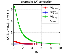
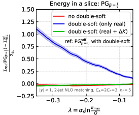
Figure 6: Left: Plot of the NLO $\Delta K$ correction, Eq. (6), for three variants of the PanGlobal shower, as a function of the rapidity $\bar{\eta}_{1}$ of a soft emission from a back-to-back dipole. $K_{\textsc{cmw}}$ is given for reference. Centre/right: impact of different parts of the double-soft correction on the NSL contributions for the transverse energy in a slice, showing the difference between PG_β=0 (centre) or PG${}_{\beta=\frac{1}{2}}$ (right) and a reference NSL-accurate shower.

Recall that for a soft emission probability (from a $\bar{q}q$ dipole) as given in Eq. (2), NSL accuracy requires an extra $(1+\Delta K\alpha_{s}/2\pi)$ correction factor. Fig. 6 (left) shows the size of the $\Delta K$ contribution, Eq. (6), for our three PanGlobal shower variants. It is plotted as a function of the rapidity, $\bar{\eta}_{1}$ of the soft emission, in the case of a back-to-back parent dipole. The shower with the largest correction is PG${}_{\beta=\frac{1}{2}}$, but for the configuration shown here, that correction remains relatively modest, at most a factor of about $(1+\alpha_{s})$ for $\bar{\eta}_{1}=0$. The correction for PG_β=0 is much smaller. The PG${}_{\beta=0}^{\text{sdf}}$ variant has the property that $\Delta K$ is identically zero, a consequence of the fact that the shower’s second emission probability is independent of the rapidity of the first emission, causing the two terms in Eq. (6) to exactly cancel.

Fig. 6 (centre and right) illustrates the separate impact of the double-soft real matrix element and $\Delta K$ corrections on the slice observable of Fig. 3, for PG_β=0 (centre) and PG${}_{\beta=\frac{1}{2}}$ (right). It shows the difference in NSL contributions between the PG_β result and an NSL-accurate reference, which is taken to be the PG${}_{\beta=0}^{\text{sdf}}$ shower including the full double-soft corrections. The red curve shows the difference with no double soft corrections at all, illustrating e.g. the fortuitous near agreement with the full NSL result for PG${}_{\beta=\frac{1}{2}}$. Turning on the real double-soft corrections (blue curve) introduces a highly visible effect, bringing the PG_β=0 result in better agreement with the full NSL but causing a significant departure from NSL in the PG${}_{\beta=\frac{1}{2}}$ case. Including also the $\Delta K$ correction (green curve) results in agreement with the NSL result for both showers. The sign of the $\Delta K$ effect is consistent with the left-hand plot: $\Delta K$ is always positive, and the resulting higher emission probability reduces the value of $\Sigma$.

Finally, let us comment on the numerical accuracy of our results. For $\lambda=-0.35$, we find $\Sigma_{\text{{nsl}}}/\Sigma_{\text{{sl}}}=4.832\pm 0.004$ (PG${}_{\beta=0}^{\text{sdf}}$), $4.817\pm 0.010$ (PG_β=0) and $4.787\pm 0.014$ (PG${}_{\beta=\frac{1}{2}}$), where the quoted uncertainties are purely statistical, as obtained from a cubic polynomial extrapolation $\alpha_{s}\to 0$. These numbers are roughly within $2\sigma$ of each other. Note however that for PG${}_{\beta=\frac{1}{2}}$, we found the convergence with $\alpha_{s}$ to be slower, making the extraction numerically more challenging. Accordingly, one should also keep in mind that this comes with additional systematic effects. For example, we observed that varying the set of $\alpha_{s}$ values yields variations in $\Sigma_{\text{{nsl}}}/\Sigma_{\text{{sl}}}$ of the order of $0.01$. We also estimated the effect of varying $\Delta K$ within its numerical uncertainty to be of order $0.005$. In all cases, we see a convincing agreement to within $1\%$ relative to the size of the NSL correction.

.3 Reference NSL results for non-global logarithms

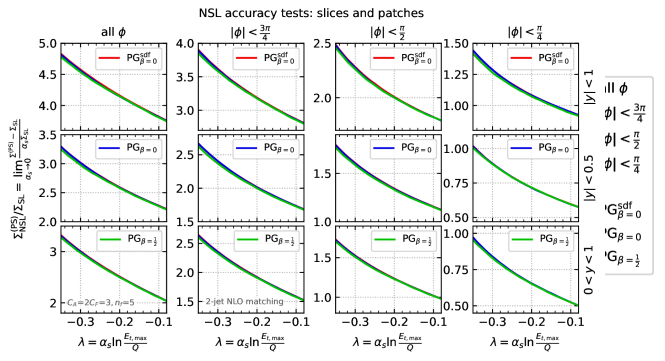
Figure 7: Next-to-single non-global logarithms contributions for the transverse energy in patches of given rapidity and azimuthal angle range. Each panel corresponds to a fixed rapidity acceptance and shows different ranges in azimuthal angle (different colours) as well as each of the three PanGlobal showers including double-soft corrections (different line styles).

In this last section, we provide additional results for non-global observables. We consider the transverse energy in a square patch of fixed extent in rapidity and azimuthal angle. In each case, we study the next-to-single logarithmic contribution, normalised to the single-logarithmic result, $\Sigma_{\text{{nsl}}}/\Sigma_{\text{{sl}}}$. We have extracted $\Sigma_{\text{{nsl}}}$ using the same variants of the PanGlobal shower as in the main text. Our results are presented in Fig. 7, showing an excellent degree of agreement, at the 1-2% level, between the showers across the whole set of observables. These can also serve as reference results for future studies of non-global logarithms at NSL accuracy.