Contrastive Graph Pooling for Explainable Classification of Brain Networks

Abstract

Functional magnetic resonance imaging (fMRI) is a commonly used technique to measure neural activation. Its application has been particularly important in identifying underlying neurodegenerative conditions such as Parkinson’s, Alzheimer’s, and Autism. Recent analysis of fMRI data models the brain as a graph and extracts features by graph neural networks (GNNs). However, the unique characteristics of fMRI data require a special design of GNN. Tailoring GNN to generate effective and domain-explainable features remains challenging. In this paper, we propose a contrastive dual-attention block and a differentiable graph pooling method called ContrastPool to better utilize GNN for brain networks, meeting fMRI-specific requirements. We apply our method to 5 resting-state fMRI brain network datasets of 3 diseases and demonstrate its superiority over state-of-the-art baselines. Our case study confirms that the patterns extracted by our method match the domain knowledge in neuroscience literature, and disclose direct and interesting insights. Our contributions underscore the potential of ContrastPool for advancing the understanding of brain networks and neurodegenerative conditions.

I Introduction

Functional magnetic resonance imaging (fMRI) measures neural activation and has been widely used in analyzing functional connectivities of the human brain [1]. Particularly, fMRI has been instrumental in identifying underlying neurodegenerative conditions [2], e.g., Alzheimer’s, Parkinson’s, and Autism.

A line of research in analyzing fMRI data models brains as graphs, i.e., defining brain regions of interest (ROIs) as nodes and the functional connectivities/interactions between ROIs as edges [3]. Graph analytics methods are then applied to such brain networks to understand and analyze the elements and interactions of neurological systems from a network perspective. While previous research has showcased the remarkable potential of network-based approaches [4, 5] in deciphering the complexities of the brain, graph analytics for brain networks is still an emerging field in its early stages of development.

Recently graph neural networks (GNNs) have attracted increasing interest in graph classification and thus have been applied to graph-structured data in a wide range of applications, including social networks [6], molecular data [7] and recommendation systems [8]. Compared with conventional machine learning models that handle vector-based data, GNNs are able to engage graph topological information through message passing. In light of the promising performance of GNNs on other applications, several studies [9, 10, 11] have applied GNNs to brain network analysis. However, directly applying general-purpose GNNs to brain networks could be ineffective on fMRI data due to its unique data characteristics [12]. (1) Low signal-to-noise ratio. fMRI is a type of high dimensional data, while non-neural noise derived from cardiac/respiratory processes or scanner instability could cause large variations within a single subject and across different subjects. (2) Node alignment. Different from other graph-based datasets, each node of a brain network represents an ROI under a brain parcellation scheme. If the same scheme is applied to all subjects, each resulting network will have the same number of nodes and the nodes are aligned across different subjects. (3) Limited data scale. Due to the limited availability of the fMRI data, brain network datasets contain a relatively small number of subjects, which can cause overfitting for GNNs.

To better utilize GNNs for brain networks and meet the need of fMRI characteristics, we propose a contrastive graph pooling method (ContrastPool) with a contrastive dual-attention to extract group-specific information. The ROI-wise attention is introduced to identify the most discriminative regions and filter out noise. The subject-wise attention utilizes the characteristic of node alignment for brain networks. With group aggregation, we obtain a contrast graph and use it to guide message passing. The group knowledge can weaken the sensitivity to specific subjects to remit overfitting. Our key contributions are:

• We propose a contrastive dual-attention block, which adaptively assigns a weight to each ROI of each subject. By aggregating subjects in each group, we introduce a differentiable graph pooling method called ContrastPool to select the most discriminative regions w.r.t different groups.

• We apply our ContrastPool to 5 resting-state fMRI brain network datasets spanning over 3 diseases. The results justify the superiority of ContrastPool over the state-of-the-art baselines.

• The case study confirms the interestingness, simplicity and high explainability of the patterns extracted by our method, which match the domain knowledge in neuroscience literature.

II Related Work

In recent years, several GNN-based methods have been proposed for brain networks. [9] leverages graph convolutional networks (GCNs) for learning similarities between each pair of graphs (subjects). [4] proposes edge-to-edge, edge-to-node and node-to-graph convolutional filters to leverage the topological information of brain networks in the neural network. [13] puts forward a two-stage pipeline to discover ASD brain biomarkers from task-fMRI using GNNs. [11] proposes an ROI-selection pooling to highlight salient ROIs for each individual. These works neglect the aforementioned three characteristics of fMRI data. Besides, [10] proposes a graph pooling method with group-level regularization to guarantee group-level consistency. [12] jointly learns the node grouping and extracts graph features. These two methods only take group information into account at the graph level without utilizing node alignment. [5] extracts a dense contrast subgraph to filter useful information for prediction. However, their feature extraction and subject classification treat all ROIs and all subjects equally, which could be vulnerable to noisy data. [14] incorporates local ROI-GNN and global subject-GNN guided by non-imaging data, such as gender, age, and acquisition site. The local ROI-GNN does not take the node alignment of brain networks into account. Moreover, [15] and [16] propose a graph generator to transform the raw blood-oxygen-level-dependent (BOLD) time series into task-aware brain connectivities. They model subjects as dynamic graphs, which require all subjects to have the same scan length and preferably from the same site. In contrast, our work constructs static brain networks as we operate on datasets collected from multi-sites with various acquisition lengths. A Transformer-based method [17] has been applied to brain networks to learn pairwise connection strengths among ROIs across individuals. It neglects the group information of subjects in its methodology design.

III Methodology

In this section, we first introduce the construction of brain networks and commonly-used GNN schemes for graph classification. We then elaborate the design of our proposed ContrastPool. Notation-wise, we use calligraphic letters to denote sets (e.g., $\mathcal{G}$), bold capital letters to denote matrices (e.g., $\bm{A}$), and bold lowercase letters to represent vectors (e.g., $\bm{z}$). Subscripts and superscripts are used to distinguish between different variables or parameters, while lowercase letters denote scalars. We use $\bm{A}(i,:)$ and $\bm{A}(:,j)$ to denote the $i$-th row and $j$-th column of a matrix $\bm{A}$, respectively. This notation also extends to a 3d matrix. Table I summarizes the notations used throughout the paper.

TABLE I: Notation Table

Notation	Description
$\bm{M}$	Connectivity matrix of a subject
$G$	An input graph/brain network
$\bm{A}$	Adjacency matrix of $G$
$\bm{X}$	Node feature matrix of $G$
$\mathcal{V}_{G}$	Node set of $G$
$v,u$	A node in G
$\bm{H}$	Node representations
$\bm{H}_{v}$	Node representation of $v$
$m$	Number of nodes in $G$
$\mathcal{D}$	Input dataset
$\mathcal{G}$	Input graph set
$\mathcal{Y}$	Input label set
$y_{G}$	Label of $G$
$l$	The layer index in GNN
$d$	Dimensionality of node representation $\bm{H}_{v}$
$\mathcal{G}^{TC},\mathcal{G}^{ASD}$	Graph set of TC/ASD group
$\mathcal{A}^{TC},\mathcal{A}^{ASD}$	Adjacency matrix set of TC/ASD group
$\mathcal{X}^{TC},\mathcal{X}^{ASD}$	Feature matrix set of TC/ASD group
$G_{sum}^{TC},G_{sum}^{ASD}$	Summary graph of TC/ASD group
$\bm{A}^{TC}_{sum},\bm{A}^{ASD}_{sum}$	Summary adjacency matrix of TC/ASD group
$\bm{X}^{TC}_{sum},\bm{X}^{ASD}_{sum}$	Summary feature matrix of TC/ASD group
$G_{contrast}$	Contrast graph
$\bm{A}_{contrast}$	Adjacency matrix of $G_{contrast}$
$\bm{H}_{contrast}$	Node representations of $G_{contrast}$
$\bm{W}_{Q},\bm{W}_{K},\bm{W}_{V}$	Parameter matrix
$i,j$	Index for matrix dimensions
$n^{TC}$	Number of subjects in TC group
$\bm{T}_{ROI}^{TC}$	Output 3d matrix of $\operatorname{Attn}_{ROI}(\cdot)$ for TC group
$\bm{T}_{subject}^{TC}$	Output 3d matrix of $\operatorname{Attn}_{subject}(\cdot)$ for TC group
$\bm{S}$	Cluster assignment matrix
$\bm{Z}$	Embedded node feature matrix
$\bm{A}_{contrast}(i,:)$	The $i$-th row of $\bm{A}_{contrast}$

III-A Preliminaries

Brain Network Construction. We construct five brain network datasets from five neuro-imaging data sources, which are Taowu, PPMI and Neurocon [18] for Parkinson’s disease, ADNI [19] for Alzheimer’s disease, and ABIDE [20] for Autism.

[TaoWu and Neurocon] The TaoWu and Neurocon datasets, released by ICI [18], are among the earliest image datasets made available for Parkinson’s research. These datasets comprise age-matched subjects collected from a single machine and site, encompassing both normal control individuals and patients diagnosed with PD.

[PPMI] The Parkinson’s Progression Markers Initiative (PPMI) is a comprehensive study aiming to identify biological markers associated with Parkinson’s risk, onset, and progression. PPMI comprises multimodal and multi-site MRI images. The dataset consists of subjects from 4 distinct classes: normal control (NC), scans without evidence of dopaminergic deficit (SWEDD), prodromal, and Parkinson’s disease (PD). This ongoing study plays a crucial role in advancing our understanding of Parkinson’s disease.

[ADNI] The ADNI raw images used in this paper were obtained from the Alzheimer’s Disease Neuroimaging Initiative (ADNI) database (adni.loni.usc.edu). The ADNI was launched in 2003 as a public-private partnership, led by Principal Investigator Michael W. Weiner, MD. The primary goal of ADNI has been to test whether serial magnetic resonance imaging (MRI), positron emission tomography (PET), other biological markers, and clinical and neuropsychological assessment can be combined to measure the progression of mild cognitive impairment (MCI) and early Alzheimer’s disease (AD). For up-to-date information, see www.adni-info.org. We included subjects from 6 different stages of AD, from cognitive normal (CN), significant memory concern (SMC), mild cognitive impairment (MCI), early MCI (EMCI), late MCI (LMCI) to Alzheimer’s disease (AD).

[ABIDE] The Autism Brain Imaging Data Exchange (ABIDE) initiative supports the research on Autism Spectrum Disorder (ASD) by aggregating functional brain imaging data from laboratories worldwide. ASD is characterized by stereotyped behaviors, including irritability, hyperactivity, depression, and anxiety. Subjects in the dataset are classified into two groups: typical controls (TC) and individuals diagnosed with ASD.

We followed [3] in resting-state fMRI data preprocessing and brain network construction. Specifically, raw MRI images are collected from the five data sources. Each fMRI image is accompanied with a structural T1-weighted (T1w) image acquired from the same subject in the same scan session. The fMRI images are then preprocessed using fMRIPrep [21], with T1w used to extract the brain mask and perform image alignment and normalization of BOLD signals. The preprocessing involves a number of pipeline steps, including motion correction, realigning, field unwarping, normalization, bias field correction, and brain extraction. Schaefer atlas [22] is applied to the preprocessed images to parcellate the brain into 100 regions of interest (ROIs). A brain network is constructed for each subject, which is represented by a connectivity matrix $\bm{M}$. The nodes in $\bm{M}$ are ROIs and the edges are the Pearson’s correlation between the region-averaged BOLD signals from pairs of ROIs. Essentially, $\bm{M}$ captures functional relationships between different ROIs. Statistics of the brain network datasets are summarized in Table II.

TABLE II: Statistics of Brain Network Datasets.

Dataset	Condition	Graph#	Avg BOLD length	Class#
Taowu	Parkinson	40	239	2
PPMI	Parkinson	209	198	4
Neurocon	Parkinson	41	137	2
ADNI	Alzheimer	1326	344	6
ABIDE	Autism	989	201	2

Brain Network Classification. Generally, graph classification aims to predict certain properties (i.e., class labels) of given graphs. Given a dataset of labeled graphs $\mathcal{D}=(\mathcal{G},\mathcal{Y})=\{(G,y_{G})\}$, where $y_{G}$ is the class label of a graph $G\in\mathcal{G}$, the problem of graph classification is to learn a predictive function $f$: $\mathcal{G}\rightarrow\mathcal{Y}$, which maps input graphs to their labels. Take brain networks constructed from the Autism dataset as an example. The class label set contains two labels: TC and ASD The objective of brain network classification is to learn a predictive function $f$ from a set of brain networks, expecting that $f$ also works well on unseen brain networks.

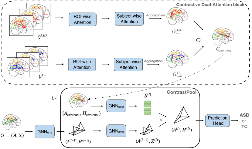
Figure 1: The architecture of ContrastPool, using Autism as an example.

Graph Neural Networks. Compared with conventional vector-based machine learning models, GNNs engage graph topological information in graph representation learning. Consider an input graph $G=(\bm{A},\bm{X})$, where $\bm{A}$ is the adjacency matrix, which encodes connectivity information, and $\bm{X}$ is the feature matrix containing attribute information for each node. The node set of $G$ is denoted as $\mathcal{V}_{G}$ and $|\mathcal{V}_{G}|=m$. The $l$-th layer of a GNN in the message-passing scheme [23] can be written as:

$$\bm{H}_{v}^{(l)}\!=\!\operatorname{AGG}^{(l-1)}\!\left(\bm{H}_{v}^{(l-1)},\operatorname{MSG}^{(l-1)}\!\left(\left\{\!\bm{H}_{u}^{(l-1)}\!\right\}_{\forall u\in\mathcal{N}(v)}\!\right)\!\right).$$ (1)

Herein, $\bm{H}^{(l)}\in\mathbb{R}^{m\times d}$ denotes the $l$-th layer node representation, where each node is represented by a $d$ dimensional vector. $\operatorname{AGG}(\cdot)$ and $\operatorname{MSG}(\cdot)$ are arbitrary differentiable aggregate and message functions (e.g., a multilayer perceptron (MLP) can be used as $\operatorname{AGG}(\cdot)$ and a summation function as $\operatorname{MSG}(\cdot)$). $\mathcal{N}(v)$ represents the neighbor node set of node $v\in\mathcal{V}_{G}$, and $\bm{H}^{(0)}_{v}=\bm{X}_{v}$. The updated representations are then passed through a sum/mean pooling and fed to a linear layer for classification. In brain network classification, we use the connectivity matrix $\bm{M}$ as both the adjacency matrix $\bm{A}$ and feature matrix $\bm{X}$. Despite prevalent, GNNs implementing Eq. (1) only propagate information across the edges of each individual brain network, and thus neglect the group-based information and node alignment. This standard message passing scheme is also vulnerable to noise as it treats all ROIs and all subjects equally important in its representation learning process. Therefore, the goal of this work is to design an end-to-end framework that addresses these limitations of GNNs when applied to brain networks.

III-B Contrastive Graph Pooling with Dual-Attention

We propose ContrastPool, which addresses the above challenges by aggregating subjects over different classes using dual-attention. The idea of ContrastPool is based on an important observation: the relatedness of different ROIs for different diseases varies, and the extent to which a subject exhibits typical characteristics of a disease also varies. Therefore, we design ContrastPool in a way that the graphs in the same group (e.g., ASD group) are summarized by assigning different weights for ROIs and subjects. These weights are not assigned manually but learnt automatically from training data to optimize the classification performance. The architecture of ContrastPool is shown in Figure 1, with Autism as an example. In the training stage, all training graphs are categorized by their groups and passed through the Contrastive Dual-Attention (CDA) block to generate the contrast graph (the upper block of Figure 1). This contrast graph is subsequently encoded into an assignment matrix, which is combined with each input graph for hierarchical graph pooling (the lower block of Figure 1). In the validation and test stages, each validation/test graph is passed through the lower block and fused with the contrast graph (generated by the training phase) to obtain its graph representation. This representation is then fed into the Prediction Head to produce the final prediction of the graph (either ASD or TC in the example).

In the following, we first introduce the Contrastive Dual-Attention block, which is used to generate a contrast graph. We then describe how the ContrastPool module produces node and graph representations based on the contrast graph. Finally, we discuss our design of the loss function.

Contrastive Dual-Attention (CDA) Block. This block aims to generate a contrast graph that best characterizes the differences in the brain networks from two groups of subjects. In order to achieve this, it first summarizes all the graphs within the same group into a summary graph. It then computes the difference of the summary graphs from two different groups. We design the computation of the summary graph as a learnable dual-attention process such that the most discriminative ROIs and the most representative subjects can be automatically highlighted in the summary graph formation.

Consider two groups of graphs in the training set, $\mathcal{G}^{TC}=(\mathcal{A}^{TC},\mathcal{X}^{TC})$ and $\mathcal{G}^{ASD}=(\mathcal{A}^{ASD},\mathcal{X}^{ASD})$, bearing TC and ASD groups, respectively. CDA first computes the summary graphs $G^{TC}_{sum}$ and $G^{ASD}_{sum}$ of the two groups via two subject aggregation functions $\operatorname{SA}_{A}(\cdot)$ and $\operatorname{SA}_{X}(\cdot)$ performed respectively on the adjacency matrix set $\mathcal{A}^{TC}$, $\mathcal{A}^{ASD}$ and the feature matrix set $\mathcal{X}^{TC}$, $\mathcal{X}^{ASD}$:

$$G^{TC}_{sum}=(\bm{A}_{sum}^{TC},\bm{X}_{sum}^{TC})=(\operatorname{SA}_{A}(\mathcal{A}^{TC}),\operatorname{SA}_{X}(\mathcal{X}^{TC})),$$ (2)

$$G^{ASD}_{sum}=(\bm{A}_{sum}^{ASD},\bm{X}_{sum}^{ASD})=(\operatorname{SA}_{A}(\mathcal{A}^{ASD}),\operatorname{SA}_{X}(\mathcal{X}^{ASD})).$$ (3)

The contrast graph $G_{contrast}=(\bm{A}_{contrast},\bm{H}_{contrast})$ is then obtained by:

$$\bm{A}_{contrast}=\bm{A}_{sum}^{TC}\ominus\bm{A}_{sum}^{ASD},$$ (4)

$$\bm{H}_{contrast}=\bm{X}_{sum}^{TC}\ominus\bm{X}_{sum}^{ASD},$$ (5)

where $\ominus$ is a binary function that computes the element-wise absolute differences of two matrices.

To enable the automatic learning of the weights on the ROIs and subjects, respectively, we design a dual-attention function as $\operatorname{SA}(\cdot)$. In general, a self-attention function [24] for a given matrix $\bm{X}\in\mathbb{R}^{k\times m}$ can be written as:

$$\operatorname{Attn}(\bm{X})=\operatorname{norm}\left(\bm{X}+\phi\left(\frac{\bm{Q}\bm{K}^{\mathsf{T}}}{\sqrt{k}}\right)\bm{V}\right),$$ (6)

$$\bm{Q}=\bm{X}\bm{W}_{Q},\bm{K}=\bm{X}\bm{W}_{K},\bm{V}=\bm{X}\bm{W}_{V},$$ (7)

where $\bm{W}_{Q},\bm{W}_{K},\bm{W}_{V}\in\mathbb{R}^{m\times m}$ are parameter matrices, $\phi(\bm{z})_{i}=\operatorname{softmax}(\bm{z})_{i}=\frac{e^{\bm{z}_{i}}}{\sum_{j=1}^{m}e^{\bm{z}_{j}}},\operatorname{for}i=1\ldots k,\bm{z}\in\mathbb{R}^{k}$, and $\operatorname{norm}(\cdot)$ is layer normalization function. Essentially, the dual-attention mechanism is performed by feeding different input matrices to Eq. (6) for different levels of attention. We illustrate the dual-attention process with $\mathcal{X}^{TC}$ as an example below. We first apply an ROI-wise attention to compute the attention between the ROIs in each subject. That is, the input matrix for the ROI-attention function $\operatorname{Attn}_{ROI}(\cdot)$ is the adjacency matrix of each subject with $k=m$. On top of this ROI-wise attention, we apply subject-wise attention to compute the attention between subjects in each ROI. The input matrix for the subject-wise attention function $\operatorname{Attn}_{subject}(\cdot)$ is the subject-stacked resultant matrix of each ROI, with a dimension of $n^{TC}\times d$, where $n_{TC}$ is the number of subjects in $\mathcal{X}^{TC}$. Finally, the output of the subject-wise attention is averaged on the subject dimension to obtain the summary feature matrix. The aggregation function $\operatorname{SA}_{X}(\cdot)$ performed on $\mathcal{X}^{TC}$ can be formally written as:

$$\bm{T}_{ROI}^{TC}=\left[\operatorname{Attn}_{ROI}\left(\bm{X}\right):\bm{X}\in\mathcal{X}^{TC}\right],$$ (8)

$$\bm{T}_{subject}^{TC}=\left[\operatorname{Attn}_{subject}\left(\bm{T}_{ROI}^{TC}(:,i,:)\right):i=1,\dots,m\right],$$ (9)

$$\operatorname{SA}_{X}(\mathcal{X}^{TC})=\frac{\sum_{j=1}^{n^{TC}}\bm{T}_{subject}^{TC}(j,:,:)}{n^{TC}},$$ (10)

where $\bm{T}_{ROI}^{TC},\bm{T}_{subject}^{TC}\in\mathbb{R}^{n^{TC}\times m\times m}$ denote two 3-dimensional matrices to store the outputs of the ROI-wise and subject-wise attention functions, and $\left[\cdot\right]$ denotes the stack function to combine a set of 2d matrices to a single 3d matrix. The subject aggregation function $\operatorname{SA}_{A}(\cdot)$ performed on the adjacency matrix sets can be defined in a similar way.

The ROI-wise attention in Eq. (8) aims to extract discriminative-related ROIs and to mitigate the influence of noise (caused by factors such as cardiac/respiratory noise or scanner instability). The goal of subject-wise attention Eq. (9) is to focus on the most representative subjects in each class. This design of dual-attention can also guarantee the permutation invariance of brain networks, which means no matter how we permute the indices of subjects or ROIs, the output will be the same.

Pooling with a Contrast Graph. This module aims to produce a high-quality representation for each input graph by leveraging the group-discriminative information captured in the contrast graph. To achieve a natural and effective utilization of the contrast graph in graph pooling and meanwhile extract high-level node features, we adopt DiffPool [25] as the pooling method. The idea is to coarsen the input graph in a hierarchical manner (via layers) such that similar nodes are grouped together into clusters at each layer to extract high-level node representations. Specifically, our ContrastPool takes the input graph with $m$ number of nodes and coarsens it by grouping the input nodes into e.g., $\frac{m}{2}$ number of clusters in a soft manner. The node grouping is performed on an embedded node feature matrix $\bm{Z}$ and guided by a cluster assignment matrix $\bm{S}$ that characterizes the node similarity. The output coarsened graph after this pooling layer contains $\frac{m}{2}$ number of nodes, with each node representing a soft cluster of the input nodes. For hierarchical pooling, $L$ number of pooling layers can be deployed.

In ContrastPool, the cluster assignment matrix can be naturally implemented by the contrast graph as it captures the relatedness of ROIs to the prediction task. As shown in Eq. (11), the contrast graph $G_{contrast}=(\bm{A}_{contrast},\bm{X}_{contrast})$ is passed through a GNN pooling, $\operatorname{GNN}^{(l)}_{pool}$, to learn a cluster assignment matrix $\bm{S}^{(l)}\in\mathbb{R}^{m^{(l-1)}\times m^{(l)}}$. Herein, $m^{(l)}$ is a pre-defined number of clusters at layer $l$ controlled by a hyperparameter named the pooling ratio.

$$\bm{S}^{(l)}=\operatorname{softmax}\left(\operatorname{GNN}_{pool}^{(l)}(\bm{A}_{contrast},\bm{X}_{contrast})\right).$$ (11)

To obtain the embedded node feature matrix $\bm{Z}^{(l)}$ at layer $l$, we pass the output graph $G^{(l-1)}=(\bm{A}^{(l-1)},\bm{H}^{(l-1)})$ from the previous layer through an embedding GNN:

$$\bm{Z}^{(l)}=\operatorname{softmax}\left(\operatorname{GNN}^{(l)}_{emb}(\bm{A}^{(l-1)},\bm{H}^{(l-1)})\right),$$ (12)

where the initial representation $\bm{H}^{(0)}$ is the input feature matrix encoded by a GNN, i.e., $\bm{H}^{(0)}=\operatorname{GNN}_{enc}(\bm{X})$.

Once we obtain the cluster assignment matrix $\bm{S}^{(l)}$ and the embedded node feature matrix $\bm{Z}^{(l)}$, we generate a coarsened adjacency matrix $\bm{A}^{(l)}$ and a new feature matrix $\bm{H}^{(l)}$. This coarsening process can reduce the number of nodes to get higher-level node representations. In particular, we apply the following two equations:

$$\bm{H}^{(l)}=\bm{S}^{(l)^{\mathsf{T}}}\bm{Z}^{(l)}\in\mathbb{R}^{m^{(l)}\times d},$$ (13)

$$\bm{A}^{(l)}=\bm{S}^{(l)^{\mathsf{T}}}\bm{A}^{(l-1)}\bm{S}^{(l)}\in\mathbb{R}^{m^{(l)}\times{m^{(l)}}}.$$ (14)

Through Eq. (13 and 14), ContrastPool is able to produce high-quality representations for each input graph by extracting high-level node representations under the guidance of the contrast graph.

Loss Function. Technically, an assignment matrix with entries close to uniform distribution could guide the GNN to treat each ROI and subsequently each node cluster produced in hierarchical pooling equally. Thus, besides the commonly-used cross-entropy loss $\mathcal{L}_{cls}$ [26] for graph classification, we also adopt the loss in [25] to regularize the entropy of the assignment matrix to avoid such equal treatment. Since a fully-connected adjacency matrix of the contrast graph could cause the over-smoothing of GNN, we apply an entropy loss to the adjacency matrix of the contrast graph $\bm{A}_{contrast}$ to sparsify the matrix. Note that imposing an entropy loss on $\bm{A}_{contrast}$ is different from thresholding the edges of $\bm{A}_{contrast}$. The former has an active impact on the learning of $\bm{A}_{contrast}$ towards the sparse formation, while the latter is a post-process on an already learnt matrix. The two entropy losses shown in Eq. (15 and 16) can help class-indicative ROIs to stand out and subsequently boost the model performance, as evidenced in our ablation study in Section IV-E.

$$\mathcal{L}_{E_{1}}=\frac{1}{L}\sum^{L}_{l=1}\frac{1}{m^{(l)}}\sum^{m^{(l)}}_{i=1}\operatorname{entropy}\left(\bm{S}^{(l)}(i,:)\right),$$ (15)

$$\mathcal{L}_{E_{2}}=\frac{1}{m}\sum^{m}_{i=1}\operatorname{entropy}\left(\bm{A}_{contrast}(i,:)\right).$$ (16)

The overall loss $\mathcal{L}$ of ContrastPool is defined as Eq. (17), where $\lambda_{1}$ and $\lambda_{2}$ are trade-off hyperparameters for balancing different losses.

$$\mathcal{L}=\mathcal{L}_{cls}+\lambda_{1}*\mathcal{L}_{E_{1}}+\lambda_{2}*\mathcal{L}_{E_{2}}.$$ (17)

IV Experimental Study

In this section, we first introduce the baseline models and the implementation details of our experiments. We then assess the performance of ContrastPool in comparison with the baseline models. We also present three case studies to show how ContrastPool meets fMRI-specific requirements, and meanwhile to provide the domain interpretation of our dual-attention mechanism. We further conduct ablation studies to analyze the effects of the components in our model. Finally, we perform sensitivity tests on the hyperparameters of our model.

IV-A Baseline Models

We select various models as baselines, including (1) conventional machine learning models: Logistic Regression, Naïve Bayes, Support Vector Machine Classifier (SVM), k-Nearest Neighbours (kNN) and Random Forest (implemented by the scikit-learn library [27]); (2) general-purposed GNNs: GCN [6], GraphSAGE [28], GIN [23], GAT [29] and GatedGCN [30]; (3) typical node clustering pooling approach, DiffPool [25]; (4) dense contrast graph with SVM: cs [5]; and (5) neural networks designed for brain networks: BrainNetCNN [4], LiNet [13], PRGNN [10], BrainGNN [11] and BNTF [17]. For GNN baseline models, we sparsify all input graphs by keeping 20% edges with top correlations in $\bm{A}$, to avoid over-smoothing.

IV-B Implementation Details

In ContrastPool, we adopt a GCN layer for $\operatorname{GNN}_{enc}$, a GraphSAGE layer for $\operatorname{GNN}_{pool}$ and $\operatorname{GNN}_{emb}$, and a sum pooling with a linear layer for the prediction head. For datasets with more than 2 groups (PPMI and ADNI), we use the most extreme groups to construct the contrast graph: CN and SMC vs. LMCI and AD for ADNI dataset; NC vs. PD for PPMI. The settings of our experiments mainly follow those in [31]. We split each dataset into 8:1:1 for training, validation and test, respectively. We evaluate each model with the same random seed under 10-fold cross-validation and report the average accuracy. The hyperparameters are grid searched by Table III.

TABLE III: Hyperparameter settings.

batch size	4 ( Taowu and Neurocon), 20 (PPMI, ADNI and ABIDE)
$\lambda_{1}$	{10, 1, 0.1}
$\lambda_{2}$	{1e-2, 1e-3, 1e-4}
pooling ratio	{0.3, 0.4, 0.5, 0.6}
L	{2, 3, 4}
learning rate	{0.02, 0.01, 0.005, 0.001}
dropout	{0, 0.1, 0.2}

The whole network is trained in an end-to-end manner using the Adam optimizer [32]. We use the early stopping criterion, i.e., we stop the training once there is no further improvement on the validation loss during 25 epochs. All the codes were implemented using PyTorch [33] and Deep Graph Library [34] packages. All experiments were conducted on a Linux server with an Intel(R) Core(TM) i9-10940X CPU (3.30GHz), a GeForce GTX 3090 GPU, and a 125GB RAM.

TABLE IV: Graph Classification Results (Average Accuracy ± Standard Deviation) over 10-fold-CV. The best result is highlighted in bold. The second best result is underlined.

	Model	Taowu	PPMI	Neurocon	ADNI	ABIDE
Conventional ML methods	Logistic Regression	77.50±7.50	56.50±11.02	68.50±15.17	61.99±0.59	65.82±3.51
	Naïve Bayes	65.00±12.25	58.83±5.42	63.50±11.84	48.27±4.44	63.50±2.69
	SVM	65.00±16.58	63.67±5.11	71.50±13.93	61.77±0.25	60.67±3.61
	kNN	62.50±12.50	53.52±10.34	56.00±21.77	62.59±1.73	60.37±5.64
	Random Forest	57.50±22.50	62.23±4.22	58.50±11.19	61.77±0.25	61.18±5.01
General- purposed GNNs	GCN	60.00±29.15	54.02±9.06	59.00±20.71	61.57±0.60	60.97±2.84
	GraphSAGE	60.00±33.91	55.00±12.89	68.50±15.17	61.19±1.72	63.09±3.11
	GIN	65.00±20.00	57.90±8.12	68.50±15.17	61.87±0.38	57.02±3.88
	GAT	67.50±22.50	54.98±8.03	54.00±15.62	61.34±1.27	60.87±5.02
	GatedGCN	65.00±22.91	52.60±11.51	69.00±25.48	62.06±4.53	63.60±4.70
	DiffPool	65.00±27.84	58.00±11.00	62.50±25.62	63.80±4.64	63.75±3.16
Models for brain networks	cs	77.50±17.50	58.36±4.40	63.50±11.84	62.25±0.47	62.59±3.14
	BrainNetCNN	65.00±27.84	57.33±10.32	66.00±22.45	61.08±2.87	65.84±2.50
	LiNet	55.00±24.49	60.71±10.61	56.00±26.91	63.64±1.73	58.14±3.72
	PRGNN	67.50±31.72	58.83±6.89	63.00±23.37	60.71±2.21	60.76±4.12
	BrainGNN	67.50±25.12	61.71±6.05	56.50±23.03	61.05±1.23	62.88±2.46
	BNTF	65.00±21.08	51.60±6.15	66.00±11.97	61.94±3.11	63.70±4.84
Ours	ContrastPool	77.50±17.50	64.00±6.63	75.00±15.81	67.08±2.63	68.63±2.65

TABLE V: Results of more evaluation metrics on Taowu, Neurocon and ABIDE datasets. The best result is highlighted in bold. For multiclass datasets of ADNI and PPMI, all these metrics are the same as accuracy in Table IV.

	model	precision	recall	micro-F1	ROC-AUC
Taowu	cs	76.67 ± 25.09	81.67 ± 14.47	79.09	77.50 ± 17.50
	ContrastPool	78.33 ± 23.64	80.00 ± 25.82	79.16	77.50 ± 17.50
Neurocon	SVM	68.33 ± 29.06	85.00 ± 32.02	75.76	65.00 ± 30.00
	ContrastPool	75.83 ± 18.05	86.67 ± 20.82	79.13	68.33 ± 20.00
ABIDE	BrainNetCNN	63.79 ± 3.09	64.82 ± 4.90	64.30	66.68 ± 2.53
	ContrastPool	64.48 ± 4.08	66.10 ± 9.13	65.28	68.16 ± 3.61

IV-C Comparison with Baselines

We report the accuracy on 5 brain network datasets in Table IV. Compared with conventional ML methods, general-purposed GNNs and models for brain network do not show a significant advantage. Our ContrastPool outperforms all 17 GNN and ML baselines on all datasets. In particular, ContrastPool improves over all GNNs specifically designed for brain networks by up to 13.6%. The average improvement over GNNs is 8.39%. Apart from accuracy, we also report other evaluation metrics, including precision, recall, micro-F1, and ROC-AUC, of the top 2 models on each dataset. As shown in Table V, ContrastPool performs the best on all datasets over all these metrics except for a single case (recall on Taowu when compared with cs). Note that we do not report the additional metrics on the two multi-class datasets PPMI and ADNI in Table V. This is because in the multi-class case, all these metrics are the same as accuracy, with the superiority of ContrastPool over all baselines already demonstrated in Table IV. These experimental results demonstrate the effectiveness of our brain network oriented model design. Existing GNNs with attention mechanism, such as GAT, PRGNN, and BrainGNN, only utilize attention over ROI-level of each subject’s feature matrix. To the best of our knowledge, our ContrastPool is the first method that applies ROI- and subject-wise attention on both adjacency matrices and feature matrices.

IV-D Case Studies

In this subsection, we present three case studies for subject-wise attention, ROI-wise attention and generalization performance to showcase how ContrastPool meets the need of three characteristics of fMRI data.

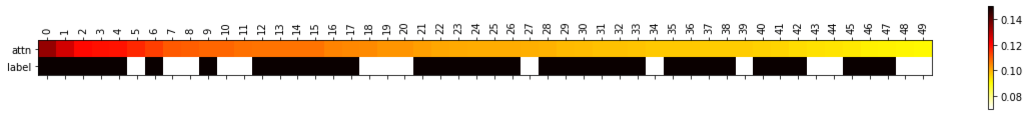
Figure 2: The heatmap to top 50 subjects in the subject-wise attention on ADNI dataset. The black and white label denotes AD and MCI subjects, respectively.

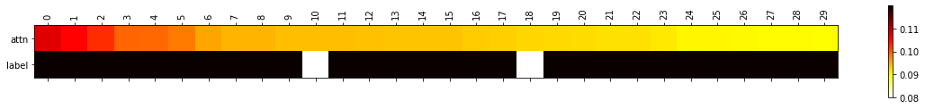
Figure 3: The heatmap to top 30 subjects in the subject-wise attention on PPMI dataset. The black and white label denotes PD and SWEDD subjects, respectively.

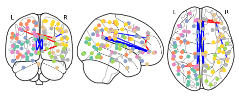
(a) ABIDE dataset. Blue edges denote higher attention on TC group and red edges denote higher attention on ASD group.

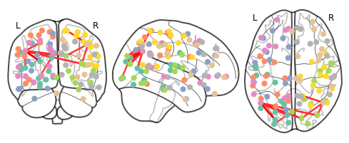
(b) ADNI dataset. Blue edges denote higher attention on CN/SMC group and red edges denote higher attention on AD/LMCI group.

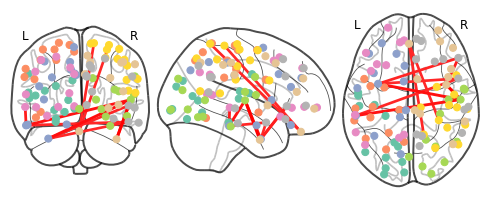
(c) PPMI dataset. Blue edges denote higher attention on NC group and red edges denote higher attention on PD group.

Figure 4: Contrast graph visualization.

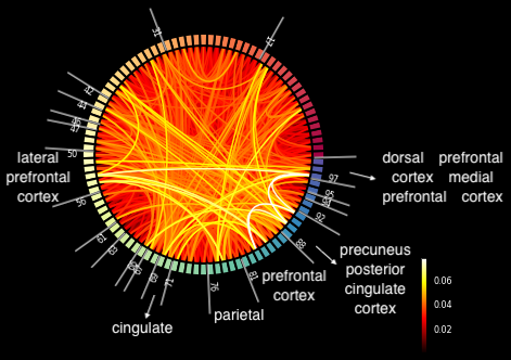
(a) ABIDE dataset.

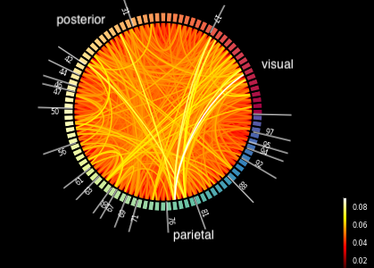
(b) ADNI dataset.

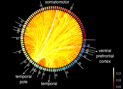
(c) PPMI dataset.

Figure 5: Chord diagrams of contrast graphs.

Subject-wise Attention. We design an experiment on ADNI dataset to demonstrate ContrastPool’s capability of underscoring informative subjects. Specifically, we merge the MCI group (82 subjects) with the AD group (143 subjects) into a single group (without revealing to ContrastPool the exact group each subject is from) to be used to contrast against the CN group. Figure 2 shows the subjects with the top 50 attention weights. The proportion of AD subjects in the top 50 attention subjects (35/50) is much higher than its proportion in the merged group of subjects (143/225). The top 5 highest attention subjects are all from the AD group. This observation illustrates that subject-wise attention could lead the model to focus more on typical/representative subjects in the dataset.

A similar conclusion can be drawn on PPMI (the other multi-class dataset) as well. We merge the SWEDD group ( 12 subjects) with the PD group (89 subjects) into a single group to be used to contrast against the NC group. Figure 3 shows the subjects with the top 30 attention weights. The proportion of PD subjects in the top 30 attention subjects (28/30) is much higher than its proportion in the merged group of subjects (89/101). The top 10 highest attention subjects are all from the PD group, which once again demonstrates the ability of ContrastPool to automatically highlight representative subjects.

Interpretation of ROI-wise Attention. To interpret the rationality of ContrastPool, we visualize the learnt contrast graphs on ABIDE, ADNI, and PPMI datasets. As shown in Figure 4, we select the edges with the top 10 attention weights. The chord diagram in Figure 5 displays the detailed attention distribution between ROIs. Take the ABIDE dataset in Figures 4(a) and 5(a) as an example. We can see that the contrast graph differentiates ROI pairs (edges in brain networks) with various importance levels (attention weights) and highlights a number of functional connections with high importance in distinguishing subjects from ASD and TC. Connections between the prefrontal cortex, parietal and cingulate are highlighted by our ROI-wise attention. Some ASD-specific neural machianism [35] may be underlying these connections, and these ROIs were regarded as key involved regions in previous ASD studies [36, 37]. Similar ROI-wise interpretations are found on Alzheimer’s and Parkinson’s as well. ROIs related to parietal and posterior are highlighted on ADNI (as shown in Figures 4(b) and 5(b)), while those within temporal and ventral prefrontal cortex are highlighted on PPMI (as shown in Figures 4(c) and 5(c)). These findings also match the domain knowledge in prior research of Alzheimer’s [38, 39, 40, 41] and Parkinson’s [42, 43, 44].

Generalization Performance. We also observe that ContrastPool is able to alleviate the overfitting problem, which is a common problem when applying GNNs to brain networks. An example is shown in Figure 6, where we plot the accuracy curves of ContrastPool and DiffPool on ABIDE dataset. The test accuracy of DiffPool decreases after its training accuracy coverages to 1. ContrastPool narrows dramatically the gap between the training and test accuracy, which demonstrates its ability in remitting the overfitting problem.

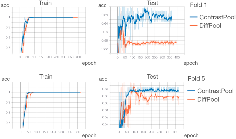
Figure 6: Accuracy curves of ContrastPool and DiffPool on two folds on ABIDE dataset.

IV-E Ablation Studies

In this subsection, we validate empirically the design choices made in different components of our model: (1) the loss function; (2) the Contrastive Dual-Attention (CDA) block. All experiments were conducted on ABIDE dataset.

Loss Function. We test our design of the loss function by disabling two entropy losses. As shown in Table VI, the results demonstrate that both $\mathcal{L}_{E_{1}}$ and $\mathcal{L}_{E_{2}}$ are effective in boosting the model performance.

TABLE VI: Ablation Study on Entropy Loss on ABIDE. The best result is highlighted in bold.

$\mathcal{L}_{cls}$	$\mathcal{L}_{E_{1}}$	$\mathcal{L}_{E_{2}}$	acc ± std
✓			64.88 ± 4.45
✓	✓		66.13 ± 2.65
✓	✓	✓	68.63 ± 2.65

CDA Block. Our CDA block performs dual attention (subject-wise and ROI-wise) on both adjacency matrices and feature matrices. We disable each of them to inspect their effects. The results reported in Table VII demonstrate that the CDA with all components enabled achieves the best performance. In particular, if the dual attention is entirely disabled (row 1), the summary graph is essentially obtained by averaging over all graphs in each group, which compromises the performance. Moreover, relying solely on ROI-wise attention (row 2) may lead to a further deterioration in performance. This implies that without the support of subject-wise attention, the ROI-wise attention suffers from the information extracted from less representative subjects.

TABLE VII: Ablation Study on CDA block on ABIDE. Winner is highlighted in bold.

Adjacency Matrices		Feature Matrices		acc ± std
subject-wise	ROI-wise	subject-wise	ROI-wise
				65.88 ± 4.11
	✓		✓	64.63 ± 3.83
✓		✓		66.25 ± 2.68
		✓	✓	66.88 ± 4.23
✓	✓			67.88 ± 4.78
✓	✓	✓	✓	68.63 ± 2.65

IV-F Hyperparameter Analysis

In this subsection, we study the sensitivity of three important hyperparameters in ContrastPool, which are the trade-off parameters in Eq. (17), the pooling ratio and the number of layers. All experiments are conducted on ABIDE dataset.

Trade-off Parameters $\lambda_{1}$ and $\lambda_{2}$. These two hyperparameters are used in the overall loss function $\mathcal{L}$ (Eq. 17) for the trade-off between the classification loss and the two entropy losses. We tune the value of $\lambda_{1}$ from 10 to 0.1 and $\lambda_{2}$ from 1e-2 to 1e-4. The results presented in Table IX show that our model performs the best when $\lambda_{1}=1$ and $\lambda_{2}=$ 1e-3. The same optimal values of $\lambda_{1}$ and $\lambda_{2}$ are found on other datasets.

TABLE VIII: Results when tuning $\lambda_{1}$ on ABIDE. The best result is highlighted in bold.

$\lambda_{1}$	acc ± std
10	68.50 ± 2.84
1	68.63 ± 2.65
0.1	66.63 ± 4.03

TABLE IX: Results when tuning $\lambda_{2}$ on ABIDE. The best result is highlighted in bold.

$\lambda_{2}$	acc ± std
1e-2	66.75 ± 4.78
1e-3	68.63 ± 2.65
1e-4	66.25 ± 5.53

Pooling Ratio. The number of nodes $m^{(l)}$ in the output graph of each ContrastPool layer is controlled by the pooling ratio. A smaller pooling ratio would lead to fewer node clusters in each ContrastPool layer. Herein, we tune it from 0.3 to 0.6 with other hyperparameters fixed. As shown in Table XI, the best choice of pooling ratio is 0.4. The best pooling ratio on different datasets varies slightly within the range of [0.4, 0.5].

TABLE X: Results when tuning pooling ratio on ABIDE. The best result is highlighted in bold.

Pool Ratio	acc ± std
0.3	66.13 ± 2.20
0.4	68.63 ± 2.65
0.5	66.25 ± 3.91
0.6	66.13 ± 3.08

TABLE XI: Results when tuning the number of layer on ABIDE. The best result is highlighted in bold.

L	acc ± std
2	68.63 ± 2.65
3	66.75 ± 4.41
4	65.00 ± 4.74

Number of Layers. The depth of the neural network can undoubtedly affect the model performance. We vary the number of layers $L$ in ContrastPool from 2 to 4, and report the results in Table XI. ContrastPool achieves the best performance when we set $L$ to 2. This indicates that by leveraging the contrast graph, our ContrastPool requires fewer layers to obtain good representations, while most other GNN baselines need to be deeper (e.g., 4 layers) to achieve best performance. The same conclusion of the optimal $L$ can be drawn on other datasets.

V Conclusion

This paper proposes a novel GNN-based solution for brain network classification, taking the unique characteristics of the underlying fMRI data into account. Our proposed method, ContrastPool, can adaptively select the most discriminative regions of interest and the most representative subjects by engaging a contrastive dual-attention block. It allows for a flexible local information aggregation within each group. We demonstrate the superiority of our method over 17 state-of-the-art baselines on 5 brain-network datasets spanning over 3 diseases. Moreover, our case studies show the interestingness, simplicity, and high explainability of the patterns extracted by our method, which find consistency in the neuroscience literature. We hope our work can inspire further research in leveraging GNNs for brain network analysis, and show significance in real-world applications, such as the early diagnosis and personalized treatments of neurodegenerative diseases.

References

- [1] K. J. Worsley, C. H. Liao, J. Aston, V. Petre, G. Duncan, F. Morales, and A. C. Evans, “A general statistical analysis for fmri data,” Neuroimage, vol. 15, no. 1, pp. 1–15, 2002.
- [2] R. A. Poldrack, Y. O. Halchenko, and S. J. Hanson, “Decoding the large-scale structure of brain function by classifying mental states across individuals,” Psychological science, vol. 20, no. 11, pp. 1364–1372, 2009.
- [3] D. T. J. Huang, S. S. Gururajapathy, Y. Ke, M. Qiao, A. Wang, H. Kumar, and Y. Yang, “Data-driven network neuroscience: On data collection and benchmark,” arXiv preprint arXiv:2211.12421, 2022.
- [4] J. Kawahara, C. J. Brown, S. P. Miller, B. G. Booth, V. Chau, R. E. Grunau, J. G. Zwicker, and G. Hamarneh, “Brainnetcnn: Convolutional neural networks for brain networks; towards predicting neurodevelopment,” NeuroImage, vol. 146, pp. 1038–1049, 2017.
- [5] T. Lanciano, F. Bonchi, and A. Gionis, “Explainable classification of brain networks via contrast subgraphs,” in Proceedings of the 26th ACM SIGKDD International Conference on Knowledge Discovery & Data Mining, 2020, pp. 3308–3318.
- [6] T. N. Kipf and M. Welling, “Semi-supervised classification with graph convolutional networks,” arXiv preprint arXiv:1609.02907, 2016.
- [7] J. Gilmer, S. S. Schoenholz, P. F. Riley, O. Vinyals, and G. E. Dahl, “Neural message passing for quantum chemistry,” in International conference on machine learning. PMLR, 2017, pp. 1263–1272.
- [8] S. Wu, F. Sun, W. Zhang, X. Xie, and B. Cui, “Graph neural networks in recommender systems: a survey,” ACM Computing Surveys, vol. 55, no. 5, pp. 1–37, 2022.
- [9] S. I. Ktena, S. Parisot, E. Ferrante, M. Rajchl, M. Lee, B. Glocker, and D. Rueckert, “Distance metric learning using graph convolutional networks: Application to functional brain networks,” in Medical Image Computing and Computer Assisted Intervention- MICCAI 2017: 20th International Conference, Quebec City, QC, Canada, September 11-13, 2017, Proceedings, Part I 20. Springer, 2017, pp. 469–477.
- [10] X. Li, Y. Zhou, N. C. Dvornek, M. Zhang, J. Zhuang, P. Ventola, and J. S. Duncan, “Pooling regularized graph neural network for fmri biomarker analysis,” in Medical Image Computing and Computer Assisted Intervention–MICCAI 2020: 23rd International Conference, Lima, Peru, October 4–8, 2020, Proceedings, Part VII 23. Springer, 2020, pp. 625–635.
- [11] X. Li, Y. Zhou, N. Dvornek, M. Zhang, S. Gao, J. Zhuang, D. Scheinost, L. H. Staib, P. Ventola, and J. S. Duncan, “Braingnn: Interpretable brain graph neural network for fmri analysis,” Medical Image Analysis, vol. 74, p. 102233, 2021.
- [12] Y. Yan, J. Zhu, M. Duda, E. Solarz, C. Sripada, and D. Koutra, “Groupinn: Grouping-based interpretable neural network for classification of limited, noisy brain data,” in proceedings of the 25th ACM SIGKDD international conference on knowledge discovery & data mining, 2019, pp. 772–782.
- [13] X. Li, N. C. Dvornek, Y. Zhou, J. Zhuang, P. Ventola, and J. S. Duncan, “Graph neural network for interpreting task-fmri biomarkers,” in Medical Image Computing and Computer Assisted Intervention–MICCAI 2019: 22nd International Conference, Shenzhen, China, October 13–17, 2019, Proceedings, Part V 22. Springer, 2019, pp. 485–493.
- [14] H. Zhang, R. Song, L. Wang, L. Zhang, D. Wang, C. Wang, and W. Zhang, “Classification of brain disorders in rs-fmri via local-to-global graph neural networks,” IEEE Transactions on Medical Imaging, 2022.
- [15] B.-H. Kim, J. C. Ye, and J.-J. Kim, “Learning dynamic graph representation of brain connectome with spatio-temporal attention,” Advances in Neural Information Processing Systems, vol. 34, pp. 4314–4327, 2021.
- [16] Y. Yu, X. Kan, H. Cui, R. Xu, Y. Zheng, X. Song, Y. Zhu, K. Zhang, R. Nabi, Y. Guo et al., “Learning task-aware effective brain connectivity for fmri analysis with graph neural networks,” arXiv preprint arXiv:2211.00261, 2022.
- [17] X. Kan, W. Dai, H. Cui, Z. Zhang, Y. Guo, and C. Yang, “Brain network transformer,” arXiv preprint arXiv:2210.06681, 2022.
- [18] L. Badea, M. Onu, T. Wu, A. Roceanu, and O. Bajenaru, “Exploring the reproducibility of functional connectivity alterations in parkinson’s disease,” PLoS One, vol. 12, no. 11, p. e0188196, 2017.
- [19] K. Dadi, M. Rahim, A. Abraham, D. Chyzhyk, M. Milham, B. Thirion, G. Varoquaux, A. D. N. Initiative et al., “Benchmarking functional connectome-based predictive models for resting-state fmri,” NeuroImage, vol. 192, pp. 115–134, 2019.
- [20] C. Craddock, Y. Benhajali, C. Chu, F. Chouinard, A. Evans, A. Jakab, B. S. Khundrakpam, J. D. Lewis, Q. Li, M. Milham et al., “The neuro bureau preprocessing initiative: open sharing of preprocessed neuroimaging data and derivatives,” Frontiers in Neuroinformatics, vol. 7, p. 27, 2013.
- [21] O. Esteban, C. J. Markiewicz, R. W. Blair, C. A. Moodie, A. I. Isik, A. Erramuzpe, J. D. Kent, M. Goncalves, E. DuPre, M. Snyder et al., “fmriprep: a robust preprocessing pipeline for functional mri,” Nature methods, vol. 16, no. 1, pp. 111–116, 2019.
- [22] A. Schaefer, R. Kong, E. M. Gordon, T. O. Laumann, X.-N. Zuo, A. J. Holmes, S. B. Eickhoff, and B. T. Yeo, “Local-global parcellation of the human cerebral cortex from intrinsic functional connectivity mri,” Cerebral cortex, vol. 28, no. 9, pp. 3095–3114, 2018.
- [23] K. Xu, W. Hu, J. Leskovec, and S. Jegelka, “How powerful are graph neural networks?” arXiv preprint arXiv:1810.00826, 2018.
- [24] A. Vaswani, N. Shazeer, N. Parmar, J. Uszkoreit, L. Jones, A. N. Gomez, Ł. Kaiser, and I. Polosukhin, “Attention is all you need,” Advances in neural information processing systems, vol. 30, 2017.
- [25] Z. Ying, J. You, C. Morris, X. Ren, W. Hamilton, and J. Leskovec, “Hierarchical graph representation learning with differentiable pooling,” Advances in neural information processing systems, vol. 31, 2018.
- [26] D. R. Cox, “The regression analysis of binary sequences,” Journal of the Royal Statistical Society: Series B (Methodological), vol. 20, no. 2, pp. 215–232, 1958.
- [27] F. Pedregosa, G. Varoquaux, A. Gramfort, V. Michel, B. Thirion, O. Grisel, M. Blondel, P. Prettenhofer, R. Weiss, V. Dubourg et al., “Scikit-learn: Machine learning in python,” the Journal of machine Learning research, vol. 12, pp. 2825–2830, 2011.
- [28] W. Hamilton, Z. Ying, and J. Leskovec, “Inductive representation learning on large graphs,” Advances in neural information processing systems, vol. 30, 2017.
- [29] P. Veličković, G. Cucurull, A. Casanova, A. Romero, P. Lio, and Y. Bengio, “Graph attention networks,” arXiv preprint arXiv:1710.10903, 2017.
- [30] X. Bresson and T. Laurent, “Residual gated graph convnets,” arXiv preprint arXiv:1711.07553, 2017.
- [31] V. P. Dwivedi, C. K. Joshi, A. T. Luu, T. Laurent, Y. Bengio, and X. Bresson, “Benchmarking graph neural networks,” arXiv preprint arXiv:2003.00982, 2020.
- [32] D. P. Kingma and J. Ba, “Adam: A method for stochastic optimization,” arXiv preprint arXiv:1412.6980, 2014.
- [33] A. Paszke, S. Gross, S. Chintala, G. Chanan, E. Yang, Z. DeVito, Z. Lin, A. Desmaison, L. Antiga, and A. Lerer, “Automatic differentiation in pytorch,” 2017.
- [34] M. Wang, L. Yu, D. Zheng, Q. Gan, Y. Gai, Z. Ye, M. Li, J. Zhou, Q. Huang, C. Ma et al., “Deep graph library: Towards efficient and scalable deep learning on graphs.” 2019.
- [35] S.-J. Weng, J. L. Wiggins, S. J. Peltier, M. Carrasco, S. Risi, C. Lord, and C. S. Monk, “Alterations of resting state functional connectivity in the default network in adolescents with autism spectrum disorders,” Brain research, vol. 1313, pp. 202–214, 2010.
- [36] M. Assaf, K. Jagannathan, V. D. Calhoun, L. Miller, M. C. Stevens, R. Sahl, J. G. O’Boyle, R. T. Schultz, and G. D. Pearlson, “Abnormal functional connectivity of default mode sub-networks in autism spectrum disorder patients,” Neuroimage, vol. 53, no. 1, pp. 247–256, 2010.
- [37] R. K. Kana, E. B. Sartin, C. Stevens Jr, H. D. Deshpande, C. Klein, M. R. Klinger, and L. G. Klinger, “Neural networks underlying language and social cognition during self-other processing in autism spectrum disorders,” Neuropsychologia, vol. 102, pp. 116–123, 2017.
- [38] R. L. Gould, R. G. Brown, A. M. Owen, E. T. Bullmore, and R. J. Howard, “Task-induced deactivations during successful paired associates learning: an effect of age but not alzheimer’s disease,” Neuroimage, vol. 31, no. 2, pp. 818–831, 2006.
- [39] M. R. Brier, J. B. Thomas, A. Z. Snyder, T. L. Benzinger, D. Zhang, M. E. Raichle, D. M. Holtzman, J. C. Morris, and B. M. Ances, “Loss of intranetwork and internetwork resting state functional connections with alzheimer’s disease progression,” Journal of Neuroscience, vol. 32, no. 26, pp. 8890–8899, 2012.
- [40] P. Alexopoulos, C. Sorg, A. Förschler, T. Grimmer, M. Skokou, A. Wohlschläger, R. Perneczky, C. Zimmer, A. Kurz, and C. Preibisch, “Perfusion abnormalities in mild cognitive impairment and mild dementia in alzheimer’s disease measured by pulsed arterial spin labeling mri,” European archives of psychiatry and clinical neuroscience, vol. 262, pp. 69–77, 2012.
- [41] S. Tu, S. Wong, J. R. Hodges, M. Irish, O. Piguet, and M. Hornberger, “Lost in spatial translation–a novel tool to objectively assess spatial disorientation in alzheimer’s disease and frontotemporal dementia,” Cortex, vol. 67, pp. 83–94, 2015.
- [42] O. Monchi, M. Petrides, J. Doyon, R. B. Postuma, K. Worsley, and A. Dagher, “Neural bases of set-shifting deficits in parkinson’s disease,” Journal of Neuroscience, vol. 24, no. 3, pp. 702–710, 2004.
- [43] N. J. Gerrits, Y. D. van der Werf, K. M. Verhoef, D. J. Veltman, H. J. Groenewegen, H. W. Berendse, and O. A. van den Heuvel, “Compensatory fronto-parietal hyperactivation during set-shifting in unmedicated patients with parkinson’s disease,” Neuropsychologia, vol. 68, pp. 107–116, 2015.
- [44] M. A. Fernández-Seara, E. Mengual, M. Vidorreta, G. Castellanos, J. Irigoyen, E. Erro, and M. A. Pastor, “Resting state functional connectivity of the subthalamic nucleus in p arkinson’s disease assessed using arterial spin-labeled perfusion f mri,” Human brain mapping, vol. 36, no. 5, pp. 1937–1950, 2015.