Synthetic Control Methods by Density Matching under Implicit Endogeneity

Abstract

Synthetic control methods (SCMs) have become a crucial tool for causal inference in comparative case studies. The fundamental idea of SCMs is to estimate counterfactual outcomes for a treated unit by using a weighted sum of observed outcomes from untreated units. The accuracy of the synthetic control (SC) is critical for estimating the causal effect, and hence, the estimation of SC weights has been the focus of much research. In this paper, we first point out that existing SCMs suffer from an implicit endogeneity problem, which is the correlation between the outcomes of untreated units and the error term in the model of a counterfactual outcome. We show that this problem yields a bias in the causal effect estimator. We then propose a novel SCM based on density matching, assuming that the density of outcomes of the treated unit can be approximated by a weighted average of the densities of untreated units (i.e., a mixture model). Based on this assumption, we estimate SC weights by matching moments of treated outcomes and the weighted sum of moments of untreated outcomes. Our proposed method has three advantages over existing methods. First, our estimator is asymptotically unbiased under the assumption of the mixture model. Second, due to the asymptotic unbiasedness, we can reduce the mean squared error for counterfactual prediction. Third, our method generates full densities of the treatment effect, not only expected values, which broadens the applicability of SCMs. We provide experimental results to demonstrate the effectiveness of our proposed method.

1 Introduction

Synthetic control methods (SCMs, Abadie & Gardeazabal, 2003; Abadie et al., 2010) have gained attention as a crucial tool for causal inference in comparative case studies across several fields, including economics, statistics, and machine learning. According to Athey & Imbens (2017), SCMs are “arguably the most important innovation in the policy evaluation literature in the last 15 years”due to their “the simplicity of the idea, and the obvious improvement over the standard methods.”

SCMs posit a scenario in which there are multiple units, with one unit being subject to a policy intervention (treated unit), at a certain time period, while the rest are not (untreated units). The focus is on estimating the causal effect of the treated unit, i.e., the difference between its observed factual and unobserved counterfactual outcome. Untreated units are used to account for unobserved trends in the outcome over time that are unrelated to the effect of the policy intervention. The key insight is that an optimally weighted average of the untreated units, referred to as the synthetic control (SC) unit, provides a more appropriate estimate of the counterfactual than estimating the counterfactual using only the treated unit. See Figure 1 for an illustration. SCMs have been applied in a variety of settings, such as the effect of terrorism on GDP (Abadie & Gardeazabal, 2003) and the decriminalization of indoor prostitution (Cunningham & Shah, 2017).

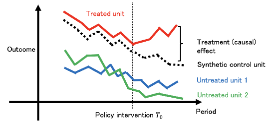
Figure 1: Illustration of SCMs.

For instance, Abadie et al. (2010) uses SCMs to study a causal effect of a comprehensive tobacco control program implemented in California in 1988. Smoking rates in California decreased following the program’s implementation, but it was unclear if this decrease was a result of the program or a long-term trend. To investigate the causal effect, as untreated units, they use annual per-capita cigarette sales data across several states that did not implement a similar tobacco control program. They then applied SCMs to estimate California’s counterfactual outcome: the smoking rate in California in 1989 if the tobacco control program had not been implemented. For further details, also see Abadie (2021).

There is a significant challenge in SCMs. In existing studies, it is typically assumed that the expected outcome of the treated unit can be represented by the weighted sum of untreated units. However, in the linear regression model deduced from the assumption, there is a correlation between the outcomes of untreated units and the error term of the SC, under which standard SCMs are not consistent (asymptotically biased), except for several specific cases (Ferman & Pinto, 2021). Remarkably, this problem is the same as the endogeneity caused by measurement error (Greene, 2003). We refer to this endogeneity as implicit endogeneity, which, to the best of our knowledge, has not been explicitly dicussed in existing literature.

To address this issue, we assume a mixture model instead of a linear relationship between expected outcomes. Specifically, we assume that the density of the outcome of the treated unit can be approximated by a linear combination of those of the untreated units. This mixture model assumption also implies that each moment of the outcome of the treated unit can be represented by a linear combination of those of the untreated units. Therefore, we can estimate the SC weights by matching moments between the outcome of the treated unit and those of the untreated units, using generalized method of moments (GMM). Unlike existing methods, our proposed estimator is asymptotically unbiased. We validate the efficacy of our proposed method through simulation studies and empirical analysis.

The use of mixture models has a close relationship with linear factor models and linear relationship between expected outcomes, assumed in existing studies (Abadie, 2021). We justify the use of the former by employing arguments from Shi et al. (2022) and Nazaret et al. (2023). Our proposed method can be considered as a new interpretation of existing SCMs. By reinterpreting existing SCMs through density matching, in addition to the implicit endogeneity problem, we address two problems in the SCM literature. First, our proposed method improves the pretreatment fit by debiasing the estimator. Second, our method generates full counterfactual densities of the treated unit, rather than the expected value. As a result, we can conduct causal inference on the distribution, or any function of the distribution, such as quantiles (Gunsilius, 2023), Lorenz curves (Gastwirth, 1971), and expected social welfare (Abadie, 2002).

Organization of the paper. In Section 2, we formulate the problem setting of treatment effect estimation. In Section 3, we point out the problem of implicit endogeneity. Then, in Section 4, we propose our method under the assumption of mixture models and GMM. In Section 5, we present a statistical inference method for our proposed method. We numerically investigate the performance of the proposed estimators through extensive simulations in Section 6.

2 Problem Setting

Suppose that there are $J+1$ units, $j\in\mathcal{J}:=\{0,1,2,\dots,J\}$, and a time series $t\in\mathcal{T}=\{1,2,\dots,T\}$ for $3\leq T\in\mathbb{N}$. Without loss of generality, we assume that the first unit ($j=0$) is the treated unit, that is, the unit affected by the policy intervention of interest. A set of potential comparisons, $j\in\mathcal{J}^{U}:=\mathcal{J}\backslash\{0\}=\{1,2,\dots,J\}$, is a collection of untreated units not affected by the intervention. We assume also that our data span $T$ periods and that the intervention occurs at $t=T_{0}$ such that $2\leq T_{0}<T$. Observations at period $t\in\mathcal{T}_{0}:=\{1,2,\dots,T_{0}\}$ are ones before the intervention, and observations at period $t\in\mathcal{T}_{1}:=\mathcal{T}\backslash\mathcal{T}_{0}$ are ones after the intervention. Let $T_{1}:=|\mathcal{T}_{1}|=T-T_{0}$.

2.1 Potential Outcomes

Following the Neyma-Rubin causal model, we formulate our problem using potential outcomes (Neyman, 1923; Rubin, 1974). For each unit $j\in\mathcal{J}$ and period $t\in\mathcal{T}$, there exist potential outcomes of interest, $\left(Y^{I}_{j,t},Y^{N}_{j,t}\right)\in\mathbb{R}^{2}$, which correspond to outcomes with and without interventions. Note that once a unit is intervened, we can only observe $Y^{I}_{j,t}$, and if a unit is not intervened, we can only observe $Y^{N}_{j,t}$. Because events that intervene and do not intervene are disjoint, we cannot observe both $Y^{I}_{j,t}$ and $Y^{N}_{j,t}$. In this sense, $\left(Y^{I}_{j,t},Y^{N}_{j,t}\right)$ are called pontential outcomes. For each $j\in\mathcal{J}$ and $t\in\mathcal{T}$, let $p^{I}_{j,t}(y)$ and $p^{N}_{j,t}(y)$ be the probability density functions (PDFs) of $Y^{I}_{j,t}$ and $Y^{N}_{j,t}$, respectively.

2.2 Observations

For each unit $j\in\mathcal{J}$, we can only observe one of the outcomes corresponding to actual intervention; that is, we observe $Y_{j,t}\in\mathbb{R}$ such that

$$Y_{0,t}=\begin{cases}Y^{N}_{0,t}&\forall t\in\mathcal{T}_{0}\\ Y^{I}_{0,t}&\forall t\in\mathcal{T}_{1}\end{cases},\qquad\mathrm{and}$$

$$Y_{j,t}=Y^{N}_{j,t}\qquad\forall j\in\mathcal{J}^{U},\ \forall t\in\mathcal{T}.$$

We are interested in estimating the effect of the intervention by predicting $Y^{I}_{0,t}$ from $(Y^{N}_{j,t})_{j\in\mathcal{J}^{U}}$ and take the difference between the predictor and observed $Y^{N}_{0,t}$ for $t\in\mathcal{T}_{1}$.

2.3 Causal Effects

We define the causal effect of the intervention for the treated unit in period $t\in\mathcal{T}_{1}$ more formally.

Average Treatment Effect on the Treated (ATT). We first consider the ATT defined as

$$\tau_{0,t}=\mathbb{E}_{0,t}\left[Y^{I}_{0,t}-Y^{N}_{0,t}\right],$$

where $\mathbb{E}_{j,t}$ denotes an expectation over a density $p_{j,t}$. Comparative case studies aim to evaluate $\tau_{0,t}$ by predicting $Y^{N}_{0,t}$ for $t>T_{0}$, which is a counterfactual outcome that would have been observed for the treated unit in the absence of the intervention. By definition, $Y^{N}_{0,t}$ is a counterfactual outcome because of the intervention after $t=T_{0}$. We usually use one unit or a small number of units that have similar characteristics as the treated unit at the time of the intervention but are not exposed to the intervention. However, when the data consist of a few units, such as regions or countries, it is often difficult to find a single untreated unit that provides a suitable comparison for the unit treated by the policy intervention of interest.

Distributional Treatment Effects (DTEs). In causal inference, we are often interested in the distributions of the outcomes (Maier, 2011) or their functionals, such as the quantile treatment effects (QTEs) and expected social welfare (Abadie, 2002), and not just the scalar treatment effect (functionals of distributions include the ATT). In this study, we consider estimating $p^{I}_{0,t}(y)$ and $p^{N}_{0,t}(y)$ for $t\in\mathcal{T}_{1}$, where outcomes corresponding to $p^{I}_{0,t}(y)$ are unobservable. Then, the treatment effect is captured by $p^{I}_{0,t}(y)$ and $p^{N}_{0,t}(y)$ themselves or functionals of $p^{I}_{0,t}(y)$ and $p^{N}_{0,t}(y)$, such as QTEs, and expected social welfare. Depending on the application, we can alter the target density, e.g., $\overline{p}^{N}_{0}(y)=\frac{1}{T_{1}}\sum_{t\in\mathcal{T}_{1}}p^{N}_{0,t}(y)$. We refer to general causal effects related to the distributions as DTEs (Park et al., 2021; Kallus & Oprescu, 2022; Chikahara et al., 2022), which includes the ATT. For example, by using some functionals $f:\mathcal{P}\to\mathbb{R}$, where $\mathcal{P}$ is a set of densities of $y$, we can define DTEs as $d_{0,t}:=f(p^{I}_{0,t})-f(p^{I}_{0,t})$. In the context of SCMs, Gunsilius (2023) and Chen (2020) estimate QTEs.

Notation.

Let us define a set $\Delta^{J-1}:=\{(w_{1},\dots,w_{J})\in\mathbb{R}^{J}|w_{j}\geq 0\ \forall j\ \mathrm{and}\ \sum_{j\in\mathcal{J}^{U}}w_{j}=1\}$. Let us define error terms as $\varepsilon_{j,t}=Y_{j,t}-\mathbb{E}_{j,t}\left[Y_{j,t}\right]$ for each $j\in\mathcal{J}$ and $t\in\mathcal{T}$. Let us define $Q^{*}$ and $\Sigma$ be $J\times J$ diagonal matrices whose $(j,j)$-element are $\frac{1}{T_{0}}\sum_{t\in\mathcal{T}_{0}}\mathbb{E}_{0,t}[\left(Y_{j,t}\right)^{2}]$ and $\mathrm{plim}\frac{1}{T_{0}}\sum_{t\in\mathcal{T}_{0}}\varepsilon^{2}_{j,t}$.

3 Identification and Implicit Endogeneity

This section describes the identification of causal effects and the problem of implicit endogeneity.

3.1 Linear Models in Expected Outcomes

In conventional SCMs, we often consider a linear relationship between $\mathbb{E}_{0,t}\left[Y_{0,t}\right]$ and $(\mathbb{E}_{j,t}\left[Y_{j,t}\right])_{j\in\mathcal{J}^{U}}$ (Ferman & Pinto, 2021; Shi et al., 2022); that is, for some $\bm{w}^{*}=(w^{*}_{j})_{j\in\mathcal{J}^{U}}\in\Delta^{J-1}$,

$$\mathbb{E}_{0,t}\left[Y_{0,t}\right]=\sum_{j\in\mathcal{J}^{U}}w^{*}_{j}\mathbb{E}_{j,t}\left[Y_{j,t}\right].$$ (1)

Under this linearity assumption, Abadie (2002) proposes the following least square estimator with a constraint to $\Delta^{J-1}$ for the SC weight $\bm{w}^{*}$ as

$$\widehat{\bm{w}}^{\mathrm{Abadie}}=\operatorname*{arg\,min}_{\bm{w}\in\Delta^{J-1}}\frac{1}{T_{0}}\sum_{t\in\mathcal{T}_{0}}\left(Y_{0,t}-\sum_{j\in\mathcal{J}^{U}}w_{j}Y_{j,t}\right)^{2}.$$

Then, the authors estimate the ATT by

$$\widehat{\tau}^{\mathrm{Abadie}}_{t}=Y^{I}_{0,t}-\widehat{Y}^{N,\mathrm{Abadie}}_{0,t},$$

where $\widehat{Y}^{N,\mathrm{Abadie}}_{0,t}=\sum_{j\in\mathcal{J}^{U}}w^{\mathrm{Abadie}}_{j}Y^{N}_{j,t}$. See also Abadie & Gardeazabal (2003); Abadie et al. (2010).

3.2 Implicit Endogeneity

Although the estimator $\bm{w}^{\mathrm{Abadie}}$ has been used in various existing studies, we find that the estimator suffers from implicit endogeneity. To understand the problem, for simplicity, instead of $\bm{w}^{\mathrm{Abadie}}$, we consider an unconstrained least-squares estimator

$$\widehat{\bm{w}}^{\mathrm{LS}}=\operatorname*{arg\,min}_{\bm{w}\in\mathbb{R}^{J}}\frac{1}{T_{0}}\sum_{t\in\mathcal{T}_{0}}\left(Y_{0,t}-\sum_{j\in\mathcal{J}^{U}}w_{j}Y_{j,t}\right)^{2}.$$

In the following, we will show that $\widehat{\bm{w}}^{\mathrm{LS}}$ is asymptotically biased.

When (1) holds, we achieve the following linear regression model:

$$Y_{0,t}=\sum_{j\in\mathcal{J}^{U}}w^{*}_{j}Y_{j,t}+\nu_{t},\quad\mathrm{where}\ \ \ \nu_{t}=-\sum_{j\in\mathcal{J}^{U}}w^{*}_{j}\varepsilon_{j,t}+\varepsilon_{0,t},$$

which is obtained by $Y_{0,t}=\mathbb{E}_{0,t}[Y_{0,t}]+\varepsilon_{0,t}=\sum_{j\in\mathcal{J}^{U}}w^{*}_{j}\mathbb{E}_{j,t}\left[Y_{j,t}\right]+\varepsilon_{0,t}=\sum_{j\in\mathcal{J}^{U}}w^{*}_{j}Y_{j,t}-\sum_{j\in\mathcal{J}^{U}}w^{*}_{j}\varepsilon_{j,t}+\varepsilon_{0,t}$. Here, note that $\mathbb{E}\left[\nu_{t}Y_{j,t}\right]\neq 0$ holds, which implies endogeneity, a correlation between the regressor and the error term. It is known that the endogeneity yields a bias in the least-squares estimator. Then, we obtain the following theorem, which directly follows from Section 5.6 of Greene (2003).

Theorem 3.1.

As $T_{0}\to\infty$, $\widehat{\bm{w}}^{\mathrm{LS}}\xrightarrow{\mathrm{p}}\overline{\bm{w}}^{\mathrm{LS}}$, where $\overline{\bm{w}}^{\mathrm{LS}}=\bm{w}^{*}-\left(Q^{*}+\Sigma\right)^{-1}\Sigma\bm{w}^{*}.$

This result implies that under the assumption of (1), there is an asymptotic bias in $\widehat{\bm{w}}^{\mathrm{LS}}$; that is, least-squares-type estimators do not converge to the true value $\bm{w}^{*}$.

3.3 Asymptotic Bias in linear factor Models

To the best of our knowledge, our study is pioneering in addressing the implicit endogeneity problem in SCMs. However, a similar issue has also been reported in Ferman & Pinto (2021). In their study, as well as Abadie (2002), the following linear factor model is analyzed:

$$Y^{N}_{j,t}=c_{j}+\delta_{t}+\lambda_{t}\mu_{j}+\varepsilon_{j,t},\quad Y^{I}_{j,t}=\tau_{j,t}+Y^{N}_{j,t},$$ (2)

$$\mathbb{E}_{j,t}[\varepsilon_{j,t}]=0,\quad\forall t\in\mathcal{T},\quad\forall j\in\mathcal{J},$$

where $\delta_{t}$ is an unobserved common factor with constant factor loadings across units, $c_{j}$ is an unknown time-invariant fixed effect, $\lambda_{t}$ is a $(1\times F)$ vector of unobserved common factors, $\mu_{j}$ is a $(F\times 1)$ vector of unknown factor loadings, and the error terms $\varepsilon_{j,t}$ are unobserved idiosyncratic shocks. Here, while $c_{j}$, $\mu_{j}$, and $\tau_{0,t}$ are non-random variables, $\delta_{t}$, $\lambda_{t}$, $\varepsilon_{j,t}$ are random variables. Under the linear factor model, the authors find that the SC estimator $\widehat{\tau}^{\mathrm{Abadie}}_{t}$ is biased for $\tau_{0,t}$ when $c_{j}$ is nonzero.

Assumption 3.2 (Common and idiosyncratic shocks).

$\frac{1}{T_{0}}\sum_{t\in\mathcal{T}_{0}}\lambda_{t}\xrightarrow{\mathrm{p}}0$, $\frac{1}{T_{0}}\sum_{t\in\mathcal{T}_{0}}\varepsilon_{t}\xrightarrow{\mathrm{p}}0$, $\frac{1}{T_{0}}\sum_{t\in\mathcal{T}_{0}}\lambda^{\top}_{t}\lambda_{t}\xrightarrow{\mathrm{p}}\Omega_{0}$ positive semidefinite, $\frac{1}{T_{0}}\sum_{t\in\mathcal{T}_{0}}\varepsilon_{t}\varepsilon^{\top}_{t}\xrightarrow{\mathrm{p}}\sigma^{2}_{\varepsilon}I_{J+1}$, and $\frac{1}{T_{0}}\sum_{t\in\mathcal{T}_{0}}\varepsilon_{t}\lambda_{t}\xrightarrow{\mathrm{p}}0$ as $T_{0}\to\infty$, where $\sigma^{2}_{\varepsilon}>0$ is a constant.

We give the statement. With a vector $\check{\bm{w}}:=(1/J,2/J,...,1/J)\in\Delta^{J-1}$, let $\widetilde{\Phi}$ be a set of SC weights $\widetilde{\Phi}:=\{\bm{w}\in\Delta^{J-1}|\mu_{0}=\sum_{j\in\mathcal{J}^{U}}w_{j}\mu_{j}\ \ \mathrm{and}\ \ c_{0}=\sum_{j\in\mathcal{J}^{U}}w_{j}c_{j}\}\backslash\{\check{\bm{w}}\}$. Then, Ferman & Pinto (2021) shows the following result.

Proposition 3.3 (Proposition 1 in Ferman & Pinto (2021)).

Suppose that $\bm{w}^{*}\in\widetilde{\Phi}$ and Assumption 3.2 hold. Then, there exists $\overline{\bm{w}}^{\mathrm{Abadie}}:=(\overline{w}^{\mathrm{Abadie}}_{j})_{j\in\mathcal{J}^{U}}\in\Delta^{J-1}\backslash\widetilde{\Phi}$ such that $\widehat{\bm{w}}^{\mathrm{Abadie}}\xrightarrow{\mathrm{p}}\overline{\bm{w}}^{\mathrm{Abadie}}$ holds. Moreover, for $t\in\mathcal{T}_{1}$, it holds that as $T_{0}\to\infty$,

$$\widehat{\tau}^{\mathrm{Abadie}}_{0,t}\xrightarrow{\mathrm{p}}\tau_{0,t}+\lambda_{t}\left(\mu_{0}-\sum_{j\in\mathcal{J}^{U}}\mu_{j}\overline{w}^{\mathrm{Abadie}}_{j}\right)+\left(c_{0}-\sum_{j\in\mathcal{J}^{U}}c_{j}\overline{w}^{\mathrm{Abadie}}_{j}\right)+\left(\varepsilon_{0,t}-\sum_{j\in\mathcal{J}^{U}}\varepsilon_{j,t}\overline{w}^{\mathrm{Abadie}}_{j}\right).$$

This result states that $\widehat{\bm{w}}^{\mathrm{Abadie}}$ does not achieve consistency. Strictly speaking, $\widehat{\bm{w}}^{\mathrm{Abadie}}$ converges to $\overline{\bm{w}}^{\mathrm{Abadie}}$ which belongs to the set that does not contain the true weight $\bm{w}^{*}$. Furthermore, since the true weight $\bm{w}^{*}$ satisfies $\mu_{0}\neq\sum_{j\in\mathcal{J}^{U}}w_{j}\mu_{j}$ and $c_{0}\neq\sum_{j\in\mathcal{J}^{U}}w_{j}c_{j}$, it also shows that $\widehat{\tau}_{0,j}^{\mathrm{Abadie}}$ does not converge to $\tau_{0,t}$.

We give a similar statement on a SC weight without the mean parameter. Let $\overline{Y}^{N}_{j}=\frac{1}{T_{0}}\sum_{t\in\mathcal{T}_{0}}Y_{j,t}$. To circumvent this issue, they propose the demeaned SC estimator

$$\widehat{\bm{w}}^{\mathrm{FP}}=(w_{1}^{\mathrm{FP}},...,w_{J}^{\mathrm{FP}})=\operatorname*{arg\,min}_{\widehat{\bm{w}}^{\mathrm{FP}}\in\Delta^{J-1}}\frac{1}{T_{0}}\sum_{t\in\mathcal{T}_{0}}\left\{\left(Y^{N}_{0,t}-\overline{Y}^{N}_{0}\right)-\sum_{j\in\mathcal{J}^{U}}w_{j}\left(Y^{N}_{j,t}-\overline{Y}^{N}_{j}\right)\right\}^{2}$$

and estimate $\tau_{0,t}$ by

$$\widehat{\tau}^{\mathrm{FP}}_{0,t}=Y^{N}_{0,t}-\overline{Y}^{N}_{0}-\sum_{j\in\mathcal{J}^{U}}\widehat{w}^{\mathrm{FP}}_{j}(Y^{N}_{j,t}-\overline{Y}^{N}_{j}).$$

Let $\Phi$ be a set of SC weights $w^{*}$ that satisfies $Y^{N}_{0,t}-c_{0}=\sum_{j\in\mathcal{J}^{U}}w^{*}_{j}\left(Y^{N}_{j,t}-c_{j}\right)$ (demeaned version of (1)); that is, $\Phi:=\{\bm{w}\in\Delta^{J-1}|\mu_{0}=\sum_{j\in\mathcal{J}^{U}}w_{j}\mu_{j}\}\backslash\{\check{\bm{w}}\}$. Then, Ferman & Pinto (2021) shows the following lemma.

Proposition 3.4 (Proposition 2 in Ferman & Pinto (2021)).

Suppose that $\bm{w}^{*}\in\Phi$ and Assumption 3.2 hold. Then, there exists $\overline{\bm{w}}^{\mathrm{FP}}:=(\overline{w}^{\mathrm{FP}}_{j})_{j\in\mathcal{J}^{U}}\in\Delta^{J-1}\backslash\Phi$ such that $\widehat{\bm{w}}^{\mathrm{FP}}\xrightarrow{\mathrm{p}}\overline{\bm{w}}^{\mathrm{FP}}$ holds. Moreover, for $t\in\mathcal{T}_{1}$, it holds that as $T_{0}\to\infty$,

$$\widehat{\tau}^{\mathrm{FP}}_{0,t}\xrightarrow{\mathrm{p}}\tau_{0,t}+\lambda_{t}\left(\mu_{0}-\sum_{j\in\mathcal{J}^{U}}\mu_{j}\overline{w}^{\mathrm{FP}}_{j}\right)+\left(\varepsilon_{0,t}-\sum_{j\in\mathcal{J}^{U}}\varepsilon_{j,t}\overline{w}^{\mathrm{FP}}_{j}\right).$$

Even if the fixed effect $c_{j}$ exists, the demeaned SC estimator is unbiased when $\mathbb{E}\left[\lambda_{t}\right]=0$. However, when $\mathbb{E}\left[\lambda_{t}\right]\neq 0$, the ATT estimator is still biased. There are two different asymptotic biases in $\widehat{\tau}^{\mathrm{Abadie}}_{0,t}$ and $\widehat{\tau}^{T,\mathrm{FP}}_{0,t}$. One of the biases is due to the existence of $c_{j}$, which is circumvented by demeaning the outcomes as $\widehat{\tau}^{T,\mathrm{FP}}_{0,t}$. However, $\widehat{\tau}^{T,\mathrm{FP}}_{0,t}$ is consistent only when $\mathbb{E}\left[\lambda_{t}\right]$. This is partly because of the implicit endogeneity. Thus, to the best of our knowledge, although the implicit endogeneity has not been clearly mentioned, similar problems have been reported by existing studies.

4 SCMs by Density Matching

As demonstrated in Section 3, the existing SCMs suffer from the implicit endogeneity problem. This issue introduces bias into the SC weight estimators when we apply least squares for weight estimation. In the other words, least squares are not compatible with SC weight estimation for (1).

To circumvent this issue, we propose novel SCMs that presume mixture models between $p_{0,t}(y)$ and $(p_{jt}(y))_{j\in\mathcal{J}^{U}}$. Then, we estimate the weights by matching the density using the GMM. We first introduce a basic SCM with mixture models, then extend it to accommodate a scenario where an additional term exists in the mixture models. The former corresponds to the original SCM proposed by Abadie (2002), and the latter corresponds to the demeaned SCM proposed by Ferman & Pinto (2021). Note that mixture models can be interpreted as linear factor models under certain conditions (Shi et al., 2022). By using the GMM under mixture models, we can sidestep the implicit endogeneity problem by appropriately estimating the weights.

4.1 Mixture Models

Our primary interest remains in predicting a counterfactual outcome $Y^{U}_{0,t}$ using a linear combination of $(Y_{j,t}){j\in\mathcal{J}^{U}}$. However, we have discussed that directly applying least squares results in a biased estimator due to the implicit endogeneity problem. That is, least squares estimator is not compatible with SC weight estimation in (1).

To avoid this problem, we propose a different estimation method by assuming mixture models on the DGP. We posit that the target distribution is a linear combination of those of the control units, expressed as

$$p^{N}_{0,t}(y)=\sum_{j\in\mathcal{J}^{U}}w^{*}_{j}p^{N}_{j,t}(y)\qquad\forall t\in\mathcal{T},$$ (3)

where $\bm{w}^{*}:=(w_{j})_{j\in\mathcal{J}^{U}}\in\Delta^{J-1}$ is an optimal weight.

Under this assumption, it follows that $\mathbb{E}_{0,t}\left[Y_{0,t}\right]=\sum_{j\in\mathcal{J}^{U}}w^{*}_{j}\mathbb{E}_{j,t}\left[Y_{j,t}\right]$.

This mixture model can be interpreted as a linear factor model when we posit fine-grained models for the DGP (Shi et al., 2022; Nazaret et al., 2023). In relation to fine-grained models, Shi et al. (2022) identifies the assumptions under which we can derive linear factor models from fine-grained models. During the arguments, we interpret the mixture models as linear factor models with $c_{j}=0$ for all $j\in\mathcal{J}$ .

4.2 Fine-Grained Models: Relationship among Mixture Models, linear factor Models, and linearity among Expected Outcomes

To elucidate the assumptions in SCMs, Shi et al. (2022) posits fine-grained models, where treated and untreated units are regarded as distributions of individuals. Based on their arguments, we can justify the assumption of mixture models by connecting them to linear factor models.

For $u\in\mathbb{N}$, let $(Y^{I}_{j,t,u},Y^{N}_{j,t,u})$ be an i.i.d. copy of $(Y^{I}_{j,t},Y^{N}_{j,t})$. Furthermore, they also suppose the existence of a $d_{W}$-dimensional unobserved random variable $W_{j,t,u}\in\mathbb{Z}^{d_{W}}$, which is an i.i.d. copy of the vector of causes $W_{j,t}\in\mathbb{Z}^{d_{W}}$ that contribute to the individual outcome of $u$, such as age, education level, or income. The relationship between the causes $W_{j,t,u}$ and potential outcomes $(Y^{I}_{j,t,u},Y^{U}_{j,t})$ can be linear or non-linear, and can also be time-variant. Let $p_{j,t}(w,y)$ and $r_{j,t}(w)$ be the PDFs of $(W_{j,t},Y^{N}_{j,t})$, and $p_{j,t}(y|w)$ be the PDF of $Y^{N}_{j,t}$ given $W_{j,t}$. The authors assume that interventions are made at a group-level and individuals in each group comply with their group-level intervention.

Then, Shi et al. (2022) finds that the following assumptions are required for the linearity of SCMs (1).

Assumption 4.1 (Independent Causal Mechanism (ICM)).

Conditional on the causes $W$, the potential outcome $Y^{N}$ is independent of the population distribution $j$. For population distribution $j$ at time $t\leq T$, the joint distribution of $Y^{M}_{j,t}$ and X is $p_{j,t}(w,y)=r_{j,t}(w)p_{t}(y|w)$.

Assumption 4.2 (Stable distributions).

Decompose the causes into two subsets $W=\{U,S\}$. Let $S$ denote the subset that differentiates the treated unit from the selected untreated units (minimal invariant set); that is, its distribution in the target unit is different from its distribution in the selected untreated units. We assume that for all groups, the distribution of $S$ does not change for all time periods $t\leq T$, $r_{j,t}(W)=\zeta_{j}(S)\xi_{t}(U|S)$.

Assumption 4.3 (Sufficiently similar untreated units).

Let $D$ be the set of untreated units used to construct the synthetic control and $S$ be the minimal invariant set for the target and untreated units. The untreated units are sufficiently similar if the cardinality of the minima invariant set, $|D|\geq|S|$.

Assumption 4.4 (Common support).

Let $(s_{1},\dots,s_{R})$ be the support of $S$. For each $s$, there exists at least one untreated unit $j$, where $\zeta_{j}(S=s)>0$.

Proposition 4.5 (Causal identifiability. From Theorem 1 of Shi et al. (2022)).

If Assumptions 4.1–4.2 hold, then there exists $\{w^{*}_{j}\}_{j\in[J]}$ such that (2) holds with $c_{j}=0$ for all $j\in\mathcal{J}$. Furthermore, in addition to Assumptions 4.1–4.2, if Assumptions 4.3 and 4.4 hold, then (3) and (1) hold.

Thus, under the results of Shi et al. (2022), if we assume fine-grained models and additional assumptions, we can relate the linear factor models to densities of units’ outcomes and show the linearity of expectation via mixture models. In other words, while we assume mixture models or fine-grained models on the DGP, the fundamental models of interest remain $\mathbb{E}_{0,t}\left[Y_{0,t}\right]=\sum_{j\in\mathcal{J}^{U}}w^{*}j\mathbb{E}{j,t}\left[Y_{j,t}\right]$ or linear factor models in (2) with $c_{j}=0$ for all $j\in\mathcal{J}$. We can interpret that fine-grained models imply linear factor models, mixture models, and $\mathbb{E}_{0,t}\left[Y_{0,t}\right]=\sum_{j\in\mathcal{J}^{U}}w^{*}j\mathbb{E}{j,t}\left[Y_{j,t}\right]$ with some assumptions. Therefore, our mixture models can be interpreted as another representation of linear factor models and $\mathbb{E}_{0,t}\left[Y_{0,t}\right]=\sum_{j\in\mathcal{J}^{U}}w^{*}j\mathbb{E}{j,t}\left[Y_{j,t}\right]$.

4.3 Weight Estimation and ATT Estimation

Under the mixture models, we employ the GMM (Hansen, 1982) to estimate the optimal weight $\bm{w}^{*}$. In this approach, we first calculate higher moments of outcomes and then estimate the weights by matching these moments.

Moment conditions.

First, we define the moment conditions that are valid under mixture models. We specify a set of $G>1$ integers, denoted as $\Gamma:={1,2,\dots,G}$.

When the outcome distribution of the treated unit can be represented as a mixture of the distributions of untreated units’ outcomes, there is a linear relationship in the higher moments as well, not just in the mean. This means that for $\gamma\in\mathbb{N}$, the moment condition is given as $m_{\gamma,t}(\bm{w}^{*})=\bm{0}$. Here, $m_{\gamma,t}:\Delta^{J-1}\to\mathbb{R}$ is a moment function defined as follows:

$$m_{\gamma,t}(\bm{w})=\mathbb{E}_{0,t}\left[\left(Y^{N}_{0,t}\right)^{\gamma}\right]-\sum_{j\in\mathcal{J}^{U}}w_{j}\mathbb{E}_{j,t}\left[\left(Y^{N}_{j,t}\right)^{\gamma}\right].$$ (4)

Then, the moment conditions are defined as $m_{\gamma,t}(\bm{w}^{*})=0$ for all $\gamma\in\Gamma$. Let us also define $\bm{m}(\bm{w})=\begin{pmatrix}\frac{1}{T_{0}}\sum_{t\in\mathcal{T}_{0}}m_{1,t}(\bm{w})&\frac{1}{T_{0}}\sum_{t\in\mathcal{T}_{0}}m_{2,t}(\bm{w})&\cdots&\frac{1}{T_{0}}\sum_{t\in\mathcal{T}_{0}}m_{G,t}(\bm{w})\end{pmatrix}^{\top}$.

Empirical moment conditions.

Further, let us define an empirical moment function $\widehat{m}_{\gamma}:\Delta^{J-1}\to\mathbb{R}$ as

$$\widehat{m}_{\gamma}(\bm{w})=\frac{1}{T_{0}}\sum_{t\in\mathcal{T}_{0}}\left\{\left(Y^{N}_{0,t}\right)^{\gamma}-\sum_{j\in\mathcal{J}^{U}}w_{j}\left(Y^{N}_{j,t}\right)^{\gamma}\right\},$$

which can be regarded as an estimator for the moment function (4). When the moment condition $m_{\gamma,t}(\bm{w}^{*})=0$ holds, we can estimate the SC weights by obtaining $\bm{w}$ such that $\widehat{m}_{\gamma}(\bm{w})=\bm{0}$ or $\widehat{m}_{\gamma}(\bm{w})$ is close to $\bm{0}$.

GMM.

We define our estimating method for the weight utilizing moment conditions in (4). Let us also define an empirical moment vector function $\widehat{\bm{m}}:\Delta^{J-1}\to\mathbb{R}^{K}$ as $\widehat{\bm{m}}(\bm{w})=\left(\widehat{m}_{1}(\bm{w}),\widehat{m}_{2}(\bm{w}),\dots,\widehat{m}_{G}(\bm{w})\right)^{\top}$. Then, we estimate SC weights as

$$\widehat{\bm{w}}^{\mathrm{GMM}}_{T_{0}}:=\left(\widehat{w}^{\mathrm{GMM}}_{j,T_{0}}\right)_{j\in\mathcal{J}^{U}}=\operatorname*{arg\,min}_{\bm{w}\in\Delta^{J-1}}\widehat{\bm{m}}^{\top}(\bm{w})\bm{V}\widehat{\bm{m}}(\bm{w}),$$ (5)

where $\bm{V}$ is some $K\times K$ matrix. By using the estimate $\widehat{\bm{w}}^{\mathrm{GMM}}_{T_{0}}$, we can estimate the ATT and DTE.

ATT estimation.

Once we estimate the weights, as well as the standard SCMs, we can estimate the ATT as

$$\widehat{\tau}^{\mathrm{DMSCM}}_{0,t}:=Y^{I}_{0,t}-\sum_{j\in\mathcal{J}^{U}}\widehat{w}^{\mathrm{GMM}}_{j,T_{0}}Y_{j,t}.$$ (6)

We refer to this estimator as the Density Matching SCM (DMSCM) estimator. In Algorithm 1, we summarize our proposed DMSCM estimator with the D2MSCM estimator introduced in the following section. Here, we need to specify $\bm{V}$. We recommend the identity matrix for $\bm{V}$ and use it in our experiments, following existing studies such as Ben-Michael et al. (2021). We can also optimize $\bm{V}$ as well as Abadie (2002) and Hansen (1982).

DTE estimation.

We can also estimate the DTE as the counterfactual distribution of $p_{0,t}(y)$ by a bootstrap method. We re-sample $L>1$ observations $\{Y^{l,\dagger}_{0}\}^{L}_{l=1}$ from $\{Y_{0,t},Y_{1,t},\dots,Y_{J,t}\}_{t\in\mathcal{T}_{1}}$ as follows: for each $l\in\mathcal{L}:=\{1,2,\dots,L\}$, (i) for each $j\in\mathcal{J}$, we re-sample $Y^{l,\dagger}_{j}$ from $\{Y_{j,t}\}_{t\in\mathcal{T}_{1}}$; (ii) we choose $Y^{l,\dagger}_{0}$ from $(Y^{l,\dagger}_{1},\dots,Y^{l,\dagger}_{J})$ with probability $(\widehat{w}^{\mathrm{GMM}}_{j,T_{0}})_{j\in\mathcal{J}^{U}}$. In this case, our focus is on $\frac{1}{T_{1}}\sum_{t\in\mathcal{T}_{1}}p_{0,t}(y)$.

Remark 4.6 (Auxiliary covariates).

We can consider a case where auxiliary covariates are observable. For each unit $j\in\mathcal{J}$, let $X_{j,t}:=(X_{j,t,1},X_{j,t,1},\dots,X_{j,t,K})\in\mathbb{R}^{K}$ be $K$-dimensional covariates, which is not affected by treatment for all $j\in\mathcal{J}$. Let $\widehat{\ell}_{k}(\bm{w})=\frac{1}{T_{0}}\sum_{t\in\mathcal{T}_{0}}\left\{X_{0,t,k}-\sum_{j\in\mathcal{J}^{U}}w_{j}X_{j,t,k}\right\}$. When the auxiliary covariates are observable, we extend the GMM estimator as $\widehat{\bm{w}}^{\mathrm{GMM}}_{T_{0}}:=\left(\widehat{w}^{\mathrm{GMM}}_{j,T_{0}}\right)_{j\in\mathcal{J}^{U}}=\operatorname*{arg\,min}_{\bm{w}\in\Delta^{J-1}}\widetilde{\bm{m}}^{\top}(\bm{w})\widetilde{\bm{V}}\widetilde{\bm{m}}(\bm{w})$, where $\widetilde{\bm{m}}(\bm{w})$ is a ($G+K$)-dimensional vector such that $\widetilde{\bm{m}}(\bm{w})=(\widehat{\bm{m}}^{\top}(\bm{w}),\widehat{\ell}_{1}(\bm{w}),\dots,\widehat{\ell}_{K}(\bm{w}))^{\top}$, and $\widetilde{\bm{V}}$ is some ($(G+K)\times(G+K)$)-dimensional matrix.

4.4 Demeaned Density Matching SCM (D2MSCM)

Next, we consider a case where the target distribution does not follow mixture models, but the deviation is zero when it is marginalized. Instead of (3), We consider the following another mixture model

$$p^{N}_{0,t}(y-c_{0})=\sum_{j\in\mathcal{J}^{U}}w^{\mathrm{GMM}*}_{j}p^{N}_{j,t}(y-c_{j})\qquad\forall t\in\mathcal{T}.$$ (7)

From the viewpoints of linear factor models 2 and fine-grained models (Shi et al., 2022), this assumption allows us $c_{j}\neq 0$ for some $j\in\mathcal{J}$. Under the previous mixture model, we only consider a case where $c_{j}=0$ for all $j\in\mathcal{J}$, which is restrictive in practice.

To estimate the SC weight, we first estimate $c_{j}$ by taking the average of $(Y_{j,t})_{t\in\mathcal{T}_{0}}$ and subtract it from $Y_{j,t}$. This manipulation corresponds to the demeaned estimation in Ferman & Pinto (2021).

Moment conditions.

Under this modeling, a moment function is defined as

$$m_{\gamma,t}(\bm{w})=\mathbb{E}_{0,t}\left[\left(Y^{N}_{0,t}-c_{0}\right)^{\gamma}\right]-\sum_{j\in\mathcal{J}^{U}}w_{j}\mathbb{E}_{j,t}\left[\left(Y^{N}_{j,t}-c_{j}\right)^{\gamma}\right].$$ (8)

We also define $\bm{m}(\bm{w})$ as well as the previous section.

Empirical moment conditions.

Then, we define an empirical moment function $\widehat{m}_{\gamma}:\Delta^{J-1}\to\mathbb{R}$ as

$$\widehat{m}_{\gamma}(\bm{w})=\frac{1}{T_{0}}\sum_{t\in\mathcal{T}_{0}}\left\{\left(Y^{N}_{0,t}-\overline{Y}^{N}_{0}\right)^{\gamma}-\sum_{j\in\mathcal{J}^{U}}w_{j}\left(Y^{N}_{j,t}-\overline{Y}^{N}_{j}\right)^{\gamma}\right\},$$ (9)

which can be regarded as an estimator for the moment function (8). Then, we estimate the SC weights by using the GMM for the empirical moment conditions.

ATT estimation.

For the GMM estimator $(\widehat{w}^{\mathrm{GMM}}_{j,T_{0}})_{j\in\mathcal{J}^{U}}$ obtained using the empirical moment condition 9, let us define

$$\widehat{w}^{\mathrm{GMM}}_{0,T_{0}}=\overline{Y}^{N}_{0}-\sum_{j\in\mathcal{J}^{U}}\widehat{w}^{\mathrm{GMM}}_{j,T_{0}}\overline{Y}^{N}_{j}.$$

By adding this term to (6), we can estimate the ATT as

$$\widehat{\tau}^{\mathrm{D2MSCM}}_{0,t}:=Y^{I}_{0,t}-\widehat{w}^{\mathrm{GMM}}_{0,T_{0}}-\sum_{j\in\mathcal{J}^{U}}\widehat{w}^{\mathrm{GMM}}_{j,T_{0}}Y_{j,t}.$$ (10)

We refer to this estimator as the Demeaned DMSCM (D2MSCM) estimator, which corresponds to the demeaned estimator of Ferman & Pinto (2021).

Algorithm 1 DMSCM and D2MSCM.

  Parameter: $\Gamma$ and $\bm{V}$.

  DMSCM: Estimates of the SC weights $\widehat{\bm{w}}^{\mathrm{GMM}}$ as (5). Then, estimate the ATT as (6).

  D2MSCM: Estimates of the SC weights $\widehat{\bm{w}}^{\mathrm{GMM}}$ with the GMM using (9). Then, estimate the ATT as (10).

4.5 Convergence of the ATT Estimators

We analyze the convergence of the proposed ATT estimators above. This analysis is important in showing that implicit endogeneity is avoided. Note that $\widehat{\tau}^{\mathrm{DMSCM}}_{0,t}$ is regarded as a special case of $\widehat{\tau}^{\mathrm{D2MSCM}}_{0,t}$, hence we only study the D2MSCM estimator $\widehat{\tau}^{\mathrm{D2MSCM}}_{0,t}$.

We first give an assumption. Let us define a population objective function as $Q(\bm{w}):=\bm{m}^{\top}(\bm{w})\bm{V}\bm{m}(\bm{w})$.

Assumption 4.7.

There exists a unique minimizer of $Q(\bm{w})$ for $\bm{w}$, denoted by $\bm{w}^{\dagger}:=\operatorname*{arg\,min}_{\bm{w}\in\Delta^{J-1}}Q(\bm{w})$, which is equivalent to $\bm{w}^{*}$.

For example, this assumption is satisfied when $\mathrm{rank}(A)=\mathrm{rank}((A,b))=J$, where

$$A=\begin{pmatrix}\mathbb{E}_{1,t}\left[\left(Y^{N}_{1,t}\right)^{1}\right]&\mathbb{E}_{2,t}\left[\left(Y^{N}_{2,t}\right)^{1}\right]&\cdots&\mathbb{E}_{J,t}\left[\left(Y^{N}_{J,t}\right)^{1}\right]\\ \mathbb{E}_{1,t}\left[\left(Y^{N}_{1,t}\right)^{2}\right]&\mathbb{E}_{2,t}\left[\left(Y^{N}_{2,t}\right)^{2}\right]&\cdots&\mathbb{E}_{J,t}\left[\left(Y^{N}_{J,t}\right)^{2}\right]\\ \vdots&\vdots&\ddots&\vdots\\ \mathbb{E}_{1,t}\left[\left(Y^{N}_{1,t}\right)^{G}\right]&\mathbb{E}_{2,t}\left[\left(Y^{N}_{2,t}\right)^{G}\right]&\cdots&\mathbb{E}_{J,t}\left[\left(Y^{N}_{J,t}\right)^{G}\right]\\ \end{pmatrix},\qquad b=\begin{pmatrix}\mathbb{E}_{0,t}\left[\left(Y^{N}_{0,t}\right)^{1}\right]\\ \mathbb{E}_{0,t}\left[\left(Y^{N}_{0,t}\right)^{2}\right]\\ \vdots\\ \mathbb{E}_{0,t}\left[\left(Y^{N}_{0,t}\right)^{G}\right]\end{pmatrix};$$

that is, there is a unique solution in the system of equation.

Under this assumption, we can prove the following theorem. The proof is shown in Appendix B.

Theorem 4.8.

Suppose that (7) and Assumption 4.7 hold, and $(Y_{j,t})_{j\in\mathcal{J},t\in\mathcal{T}}$ are stationary and ergodic. Then, as $T_{0}\to\infty$, $\widehat{\bm{w}}^{\mathrm{GMM}}\xrightarrow{\mathrm{p}}\bm{w}^{*}$, and

$$\widehat{\tau}^{\mathrm{D2MSCM}}_{0,t}\xrightarrow{\mathrm{p}}\tau_{0,t}+\left(\varepsilon_{0,t}-\sum_{j\in\mathcal{J}^{U}}w^{*}_{j}\varepsilon_{j,t}\right).$$

While the SC weight estimators converge to points other than $w^{*}$ in Propositions 3.3 and 3.4, our DMSCM and D2SCM estimators converge to $w^{*}$. Owing to this consistency, unlike in Propositions 3.3 and 3.4, there are no excess terms such as $\left(\mu_{0}-\sum_{j\in\mathcal{J}^{U}}\mu_{j}\overline{w}^{\mathrm{Abadie}}_{j}\right)$ and $\left(c_{0}-\sum_{j\in\mathcal{J}^{U}}c_{j}\overline{w}^{\mathrm{Abadie}}_{j}\right)$. As a result, $\widehat{\tau}^{\mathrm{DMSCM}}_{0,t}$ and $\widehat{\tau}^{\mathrm{D2MSCM}}_{0,t}$ are asymptotically unbiased under each respective assumption.

Remark 4.9 (Uniqueness of the weights).

Consider a case where $p_{1t}(y)$ and $p_{2t}(y)$ are densities of $\mathcal{N}(\mu_{1t},\sigma^{2}_{1})$ and $\mathcal{N}(\mu_{2t},\sigma^{2}_{2})$, where $\mu_{1t}=\mu_{2t}=0$ for all $t\in\mathcal{T}_{0}$ and $\mu_{1t}=1$, $\mu_{2t}=0$ for all $t\in\mathcal{T}_{1}$, and $\sigma^{2}_{1},\sigma^{2}_{2}>0$ are constants such that $\sigma^{2}_{1}\neq\sigma^{2}_{2}>0$. Assume that $p_{0,t}(y)=0.5p_{1t}(y)+0.5p_{2t}(y)$ In this case, we cannot specify $(w^{*}_{1},w^{*}_{2})$ because $\mathbb{E}_{0,t}[Y]=w^{*}_{1}\mathbb{E}_{0,t}[Y]+w^{*}_{2}\mathbb{E}_{0,t}[Y]=0$ for all $\bm{w}^{*}=(w^{*}_{1},w^{*}_{2})$ in pre-intervention periods. However, in $t\in\mathcal{T}_{1}$, only $w^{*}_{1}=w^{*}_{2}=0.5$ returns a valid prediction. Therefore, we cannot correctly estimate $\bm{w}^{*}$ from existing SCMs only using the relationship $\mathbb{E}_{0,t}[Y]=w^{*}_{1}\mathbb{E}_{0,t}[Y]+w^{*}_{2}\mathbb{E}_{0,t}[Y]$. However, if we include higher moment information $\mathbb{E}_{0,t}[Y^{2}]=w^{*}_{1}\mathbb{E}_{0,t}[Y^{2}]+w^{*}_{2}\mathbb{E}_{0,t}[Y^{2}]$ and $\mathbb{E}_{0,t}[Y^{4}]=w^{*}_{1}\mathbb{E}_{0,t}[Y^{4}]+w^{*}_{2}\mathbb{E}_{0,t}[Y^{4}]$, we can correctly specify $\bm{w}^{*}$ as a solution of $0.5=w^{*}_{1}+2w^{*}_{2}$ and $1=w^{*}_{1}+w^{*}_{2}$.

5 Inference

We consider statistical inference on the ATT using our proposed DMSCM and D2SCM to test the sharp null hypothesis, $H_{0}:\tau_{0,t}=\alpha_{t}$ for some $t\in\mathcal{T}_{t}$ and $\bm{\alpha}=(\alpha_{t})_{t\in\mathcal{T}_{1}}$. Note that $\tau_{0,t}=Y^{I}_{0,t}-Y^{N}_{0,t}$ under the linear factor model. Here, we focus on the conformal inference of Chernozhukov et al. (2021), which has been utilized in existing studies, such as Ben-Michael et al. (2021) and Ferman & Pinto (2021). This approach consists of the following three steps. First, for the null hypothesis $H_{0}:\tau_{0,t}=\alpha_{t}$, we create adjusted post-treatment outcomes for the treated unit $Y^{N\sharp}_{0,t}=Y^{I}_{0,t}-\alpha_{t}$ and add it to the original dataset as $(Y_{0,1},\dots,Y_{0,T_{0}},Y^{N\sharp}_{0,(T_{0}+1)},\dots,Y^{N\sharp}_{0,T})$. Then, we apply our proposed method to the extended datasets consisting of $(Y_{0,1},Y_{0,2},\dots,Y^{N\sharp}_{0,(T_{0}+1)},\dots,Y^{N\sharp}_{0,T})$ and $(Y_{j,t})_{t\in\mathcal{T},j\in\mathcal{J}^{U}}$ to obtain adjusted weights $\widehat{\bm{w}}(\alpha)$ and a corresponding predictor of the counterfactual outcome, denoted by $\widehat{Y}^{N}_{0,t}(\bm{\alpha})$. Finally, we compute the $p$-value by assessing whether the adjusted residual “conforms” with the pretreatment residuals. Let $u_{t}(\bm{\alpha})$ be the residual defined as $u_{t}(\bm{\alpha})=Y_{0,t}-\widehat{Y}^{N}_{0,t}(\bm{\alpha})$ for $t\in\mathcal{T}_{0}$ and $u_{t}(\bm{\alpha})=Y^{I}_{0,t}-\alpha_{t}-\widehat{Y}^{N}_{0,t}(\bm{\alpha})$ for $t\in\mathcal{T}_{1}$. For $j\in\mathcal{T}$, let $\pi_{j}$ be a permutation of indexes defined as $\pi_{j}(t)=t+j$ if $t+j\leq T$ and $\pi_{j}(t)=t+j-T$ otherwise. Let $\Pi=\{\pi_{1},\dots,\pi_{T-1}\}$. Then, the $p$-value is defined as $\widehat{p}(\bm{\alpha})=1-\widehat{F}(\bm{\alpha})$, where $\widehat{F}(\bm{\alpha})=\frac{1}{T}\sum_{j\in\mathcal{T}}\mathbbm{1}\Big{[}\frac{1}{T}\sum_{t\in\mathcal{T}}\left|u_{t}(\bm{\alpha})\right|<\frac{1}{T}\sum_{\pi_{j}\in\mathcal{T}}\left|u_{\pi_{j}}(\bm{\alpha})\right|\Big{]}$. Because $Y^{N}_{0,t}$ is random, by inverting this test, we can construct a confidence interval for $\tau_{0,t}$, which is equivalent to constructing a conformal prediction set (Vovk et al., 2005) for $Y^{N}_{0,T}$. The $(1-\xi)$ confidence interval is given as $\widehat{C}^{\mathrm{conf}}_{1-\xi}=\left\{\bm{\alpha}\in\mathcal{A}\big{|}\widehat{p}(\bm{\alpha})>\xi\right\}$, where $\mathcal{A}$ is a set of candidates of $\bm{a}$. For the details including theoretical conditions, see Appendix C.

Remark 5.1 (Two-sample homogeneity test).

When we are interested in the DTE, there are several ways for inference. For example, we can define the null and alternative hypotheses as $H_{0}:p^{I}_{t}=p^{N}_{t}$ and $H_{1}:p^{I}_{t}\neq p^{N}_{t}$. Then, we can conduct hypothesis testing by applying the two-sample homogeneity test, and our DTE estimator. For example, we can employ maximum mean discrepancy (MMD) for testing (Gretton et al., 2012).

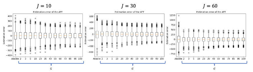
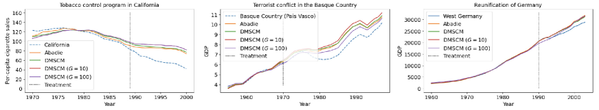
Figure 2: Results of simulation studies. Estimation errors of ATT estimation.

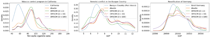
Figure 3: Counterfactual outcomes in empirical analysis.

Figure 4: Counterfactual distributions in empirical analysis.

Table 1: Results of conformal inference. Estimated ATT $\widehat{\tau}_{0,t}$ and $90\%$ confidence interval $(\underline{\tau}_{0,t},\overline{\tau}_{0,t})$.

	Terrorist conflict in Basque country					Tobacco control program in California					Reunification of Germany
	Abadie	DMSCM				Abadie	DMSCM				Abadie	DMSCM
$\gamma$	-	$2$	$5$	$10$	$100$	-	$2$	$5$	$10$	$100$	-	$2$	$5$	$10$	$100$
$\widehat{\tau}_{0,t}$	-0.800	-0.845	-1.054	-0.279	-0.138	-26.148	-27.744	-32.306	-35.080	-36.879	-1492.374	-1253.616	-1419.120	-1324.448	-510.765
$\overline{\tau}_{0,t}$	0.522	0.699	0.495	0.521	0.578	8.698	7.852	8.898	9.544	11.748	2635.583	-1008.822	-591.420	-716.376	2327.944
$\underline{\tau}_{0,t}$	-2.587	-2.150	-2.605	-2.616	-2.590	-36.798	-29.268	-34.783	-37.308	-35.243	-2390.413	-2738.232	-1989.323	-2018.878	-2625.129

6 Experiments

We conduct experiments with simulated and real-world data. Additional results are in Appendix 6.1.

6.1 Simulation Studies

In this section, we perform simulation studies to show how our proposed SCMs compared to traditional SCMs. Let $J\in\{10,30,60\}$ $G\in\{2,3,5,10,20,30,40,50,60,70,80,90,100\}$, $T_{0}=30$, $T_{1}=100$, and $K=5$. We perform a simulation on SCMs for $p_{0,t}(\bm{z})=\sum_{j\in\mathcal{J}^{U}}w^{*}_{j}p_{0,t}(\bm{z})$, where $\bm{z}$ is ($K+1$)-dimensional ($6$-dimensional) vector, where the first element corresponds to $Y_{j,t}$ and the rest corresponds to $X_{j,t}$. For each $j\in\mathcal{J}$, let $p_{j,t}$ be a density of a multinomial normal distribution $\mathcal{N}(\bm{\mu}_{j,t},\bm{\sigma}^{2}_{j,t})$, where $\bm{\mu}_{j,t}=(\mu_{j,t,1},\mu_{j,t,2},\mu_{j,t,3},\mu_{j,t,4},\mu_{j,t,5},\mu_{j,t,6})$, and $\bm{\sigma}^{2}_{j,t}$ is a $(6\times 6)$-diagonal matrix with a $(k,k)$-element denoted by $\sigma^{2}_{j,t,k}$. At period $t=0$, each mean parameter $\mu_{j,0,k}$ for $j\in\mathcal{J}$ and $k\in\{1,2,\dots,6\}$ is drawn from a standard normal; distribution. Similarly, each variance parameter $\sigma^{2}_{j,0,k}$ is drawn from a uniform distribution with support $[1,20]$. While $\mu_{j,t,k}$ and $\sigma^{2}_{j,t,k}$ are time-invariant for $k\in\{2,\dots,6\}$; that is, $\mu_{j,0,k}=\mu_{j,t,k}$ and $\sigma^{2}_{j,0,k}=\sigma^{2}_{j,t,k}$ for $t\in\mathcal{T}$ and $k\in\{2,\dots,6\}$, let $\mu_{j,t,1}$ and $\sigma^{2}_{j,t,1}$ be time-variant. For each $j\in\mathcal{J}$, we change the parameters change as $\mu_{j,t+1,1}=\mu_{j,t,1}+\epsilon_{j,t}$ and $\sigma^{2}_{j,t+1,1}=\sigma^{2}_{j,t,1}+\widetilde{\epsilon}_{j,t}$, where $\epsilon_{j,t}$ and $\widetilde{\epsilon}_{j,t}$ follow a normal densities $\mathcal{N}(0,10)$, respectively. Let us correct the variance as $\widetilde{\epsilon}_{j,t}=0.1$ if $\widetilde{\epsilon}_{j,t}\leq 0.1$ occurs. For the treated unit, we assume that $Y^{N}_{0,t}\sim p_{0,t}(\bm{z})$ for $t\in[t_{0},T_{1}]$ and $Y^{I}_{0,t}=20+Y^{N}_{0,t}$ for $t\in\mathcal{T}_{1}$; that is $\tau_{0,t}=20$. We draw $\bm{w}^{*}$ from a uniform distribution and normalize the sum to be $1$. We apply DMSCM and Abadie $1,000$ times and compute the error of the ATT estimation. We show the result with a boxplot in Figure 4. Our proposed method successfully estimates the ATT with smaller estimation errors. The estimation error decreases as $G$ increases.

6.2 Empirical Analysis

We conduct empirical studies discussed in Abadie & Gardeazabal (2003), Abadie et al. (2010), and Abadie et al. (2015). Here, we briefly explain each example, and further details are in Appendix D.

Terrorist conflict in the Basque Country. Abadie & Gardeazabal (2003) investigates the effect of terrorist conflict in the Basque Country on the gross domestic product (GDP). In this example, $J=16$, $K=14$, and $(t_{0},T_{0},T_{1})=(1955,1970,1997)$.

Tobacco control program in California. Abadie et al. (2010) study the effect of a large tobacco control program adopted in California in $1988$, which we explained in our introduction. In this example, $J=20$, $K=5$, and $(t_{0},T_{0},T_{1})=(1970,1989,2000)$.

Reunification of Germany. Abadie et al. (2015) studies the effect of the reunification of Germany on GDP in 1990. Because the countries were dissimilar from any one country to make a comparison group, they apply SCMs to create a composite comparison group. In this example, $J=8$, $K=31$, and $(t_{0},T_{0},T_{1})=(1960,1990,2003)$.

Results. We show the result of the estimated treatment effect and $90$% confidence interval in Table 1. We show the results of ATT estimation in Figure 4 and DTE estimation in Figure 4.

For each dataset, we plot the counterfactual outcomes and distributions in Figures 4 and 4, respectively. We also conduct conformal inference on the null hypothesis $H_{0}:\tau_{0,(T_{0}+1)}=\cdots=\tau_{0,T_{1}}=0$ for the ATT. For the results of Abadie, DMSCM, We show the $90\%$ confidence interval of the ATT in Table 1. Our proposed method has a good fit in terms of the observed outcomes in pretreatment periods $t\in\mathcal{T}_{0}$. Therefore, we consider that our proposed method also predicts counterfactual outcomes and distributions well. In conformal inference, our method does not reject the null hypothesis as with Abadie, except for the DMSCM in the tobacco control problem in California.

7 Conclusion

In this study, we pointed out an issue of implicit endogeneity on linear regression commonly used in existing studies about SCMs. To tackle this problem, we proposed a novel approach to SCMs utilizing density matching. This proposed method allows for consistent estimation of SC weights, thereby enhancing the precision of counterfactual outcome predictions when compared to established methods. We have validated the efficacy of our approach through simulation experiments and empirical analysis.

Appendix A Review of SCMs

To estimate the treatment effect $\tau_{0,t}$, Abadie & Gardeazabal (2003) proposes SCMs that predicts the counterfactual outcome $Y^{N}_{0,t}$ by using the weighted sum of $\{Y_{j,t}\}^{J}_{j=1}$.

In standard SCMs, weights are determined by minimizing the squared error between $Y^{N}_{0,t}$ and a weighted sum of $Y_{1t},...,Y_{j,t}$. Then, the counterfactual outcome and ATT are estimated as

$$\widehat{Y}^{N,\mathrm{std}}_{0,t}=\widehat{w}^{\mathrm{std}}_{0}+\sum_{j\in\mathcal{J}^{U}}\widehat{w}^{\mathrm{std}}_{j}Y_{j,t},$$

and $\widehat{\tau}^{\mathrm{std}}_{t}=Y_{0,t}-\widehat{Y}^{N,\mathrm{std}}_{0,t}$, where for some norm $\|\cdot\|$,

$$(\widehat{w}^{\mathrm{std}}_{0},\bm{w}^{\mathrm{std}})=\operatorname*{arg\,min}_{\bm{w}\in\Lambda}\sum_{t\in\mathcal{T}_{0}}\left\|Y_{0,t}-w_{0}-\sum_{j\in\mathcal{J}^{U}}w_{j}Y_{j,t}\right\|,$$

and $\Lambda$ is a set of weight parameters. Abadie & Gardeazabal (2003); Abadie et al. (2010) propose $\Lambda=\big{\{}w_{0}\in\mathbb{R},\bm{w}\in\Delta^{J-1}:w_{0}=0\big{\}}$. For the norm, Abadie et al. (2010) proposes the L2 norm.

Doudchenko & Imbens (2016) proposes removing the restriction $w_{0}=0$ and introducing the Elastic Net regularization.

The standard SCMs are known to be vulnerable to model misspecification. Ferman & Pinto (2021) analyzes the problem assuming the following linear factor model:

$$Y^{N}_{j,t}=c_{j}+\delta_{t}+\lambda_{t}\mu_{j}+\varepsilon_{j,t},$$

and $Y^{I}_{0,t}=\tau_{0,t}+Y^{N}_{0,t}$, where $\delta_{t}$ is an unobserved common factor with constant factor loadings across units, $c_{j}$ is an unknown time-invariant fixed effect, $\lambda_{t}$ is a $(1\times F)$ vector of unobserved common factors, $\mu_{j}$ is a $(F\times 1)$ vector of unknown factor loadings, and the error terms $\varepsilon_{j,t}$ are unobserved idiosyncratic shocks. They find that the standard SCM estimator is biased for $\tau_{0,t}$ when the fixed effect $c_{j}$ exists and propose the demeaned SCM using the following weight: $\widehat{\bm{w}}^{\mathrm{FP}}=$

$$\operatorname*{arg\,min}_{\widehat{\bm{w}}^{\mathrm{FP}}\in\Delta^{J-1}}\frac{1}{T_{0}}\sum_{t\in\mathcal{T}_{0}}\left\{\left(Y^{N}_{0,t}-\overline{Y}^{N}_{0}\right)-\sum_{j\in\mathcal{J}^{U}}w_{j}\left(Y^{N}_{j,t}-\overline{Y}^{N}_{j}\right)\right\},$$

and $\widehat{\tau}^{T,\mathrm{FP}}_{T_{0}}=Y^{N}_{0,T}-\overline{Y}^{N}_{0}-\sum_{j\in\mathcal{J}^{U}}\widehat{w}^{\mathrm{FP}}_{j}\left(Y^{N}_{j,t}-\overline{Y}^{N}_{j}\right)$, where $\overline{Y}^{N}_{j}=\frac{1}{T_{0}}\sum_{t\in\mathcal{T}_{0}}Y_{j,t}$. Even if the fixed effect $c_{j}$ exists, the demeaned SCM estimator is unbiased when $\mathbb{E}[Y^{N}_{0,t}]=\sum_{j\in\mathcal{J}^{U}}\overline{w}^{\mathrm{FP}}_{j}\mathbb{E}[Y^{N}_{j,t}]$, where $\overline{w}^{\mathrm{FP}}_{j}$ is a limit of $\widehat{w}^{\mathrm{FP}}_{j}$. For the details, see Ferman & Pinto (2021). However, when $\mathbb{E}[Y^{N}_{0,t}]\neq\sum_{j\in\mathcal{J}^{U}}\overline{w}^{\mathrm{FP}}_{j}\mathbb{E}[Y^{N}_{j,t}]$, the demeaned SCM estimator is also biased.

There is a growing literature on inference for SCMs, going beyond the original proposal in Abadie & Gardeazabal (2003) and Abadie et al. (2010); see, for example, Li (2020), Shaikh & Toulis (2021), Cattaneo et al. (2021), and Chernozhukov et al. (2019).

A.1 Other Related Work

An excellent illustration of the relevance of estimating distribution functions is Ropponen (2011), which applies the changes-in-changes estimator by Athey & Imbens (2006) to estimate the effect of minimum wage changes on employment levels in order to reconcile the classical conflicting results about the minimum wage debate in Card & Krueger (2000) and Neumark & Wascher (2000). Spiess et al. (2023) investigates high-dimensional linear regression models in SCMs.

The exploration of identification assumptions has been attempted in the existing literature. Ferman & Pinto (2021) conducts a comprehensive investigation to discern the conditions under which conditions SCMs can accurately predict counterfactual outcomes.

On a different note, Shi et al. (2022) introduces fine-grained models to investigate hidden assumptions inherent to SCMs, which also explores a connection between the linear combination of expected outcomes and the linear factor models. Nazaret et al. (2023) extends the finding into the problem of model misspecification,

The GMM has been widely used in the literature of econometrics (Hansen, 1982). The idea of the GMM is to obtain parameters that satisfy empirically approximated moment conditions, which can be applied in various fields, such as causal inference and time-series analysis. For the details, see textbooks of econometrics.

Appendix B Proofs of Theorem 4.8

First, we prove Theorem 4.8.

Proof.

Suppose that the mixture model (7) and Assumption 4.7 hold, and $(Y_{j,t})_{j\in\mathcal{J},t\in\mathcal{T}}$ are stationary and ergodic. Furthermore, from the definition of $\Delta^{J-1}$, $\Delta^{J-1}$ is a compact parameter space. Therefore, from Theorem 2.1 of Hansen (1982), the claim holds. ∎

Note that the uniqueness assumption (Assumption 4.7) can be replaced by the continuous differentiability of $Q(\bm{w})$ around $\bm{w}_{0}$ (local identification) if we are not interested in a unique solution.

Appendix C Conformal Inference

Our goal is to establish a confidence interval whose $p$-value $\widehat{p}$ satisfies that for any $a\in(0,1)$,

$$\mathrm{Pr}(\widehat{p}\leq a)\to a$$ (11)

as $T_{0}\to\infty$ and $T_{1}$ is fixed.

We can prove (11) by using Theorem 1 of Chernozhukov et al. (2021); that is, if the following assumptions hold, (11) holds.

Assumption C.1 (Counterfactual model).

Let $\{P^{N}_{0,t}\}$ be a given sequence of mean-unbiased predictors or proxies for the counterfactual outcomes $\{Y^{N}_{0,t}\}$ in the absence of the policy intervention, that is $\{\mathbb{E}_{0,t}\left[P^{N}_{0,t}\right]\}=\{\mathbb{E}_{0,t}\left[Y^{N}_{0,t}\right]\}$. In other words, potential outcomes can be written as

$$\begin{array}[]{l}Y_{0,t}^{N}=P^{N}_{0,t}+\varepsilon_{0,t}\\ Y_{0,t}^{I}=P^{N}_{0,t}+\tau_{0,t}+\varepsilon_{0,t}\\ \end{array},\qquad\mathbb{E}[\varepsilon_{0,t}]=0,\quad t\in\mathcal{T},$$

where $\{\varepsilon_{0,t}\}$ is a centered stationary stochastic process.

Assumption C.2 (Regularity of the stochastic shock process).

Assume that the density function of $S(\varepsilon_{0,t})$ exists and is bounded, and that the stochastic process $\{\varepsilon_{0,t}\}_{t=1}^{T}$ are stationary, strongly mixing, with the sum of mixing coefficient bounded by $M$.

Let $\widehat{P}^{N}_{0,t}$ be $\widehat{\tau}^{\mathrm{D2MSCM}}_{0,t}$ or $\widehat{\tau}^{\mathrm{D2MSCM}}_{0,t}$.

Assumption C.3 (Consistency of the counterfactual estimators under the null).

Let there be sequences of constants $\delta_{T}$ and $\gamma_{T}$ converging to zero. Assume that with probability $1-\gamma_{T}$,

1. the mean squared estimation error is small, $\|\widehat{P}^{N}_{0,t}-P^{N}_{0,t}\|^{2}_{2}/T\leq\delta^{2}_{T}$;

2. for $t\in\mathcal{T}_{1}$, the pointwise errors are small, $|\widehat{P}^{N}_{0,t}-P^{N}_{0,t}|\leq\delta_{T}$.

Therefore, to show (11), we need to confirm that the other assumptions hold. Firstly, we assume that (C.2) holds. If the mixture model or the linear factor model hold, Assumption 11 holds. For our proposed methods, Theorem 4.8 implies that C.3. Thus, the claim holds.

Appendix D Experiments

In this section, we report additional experimental results and details of the datasets used.

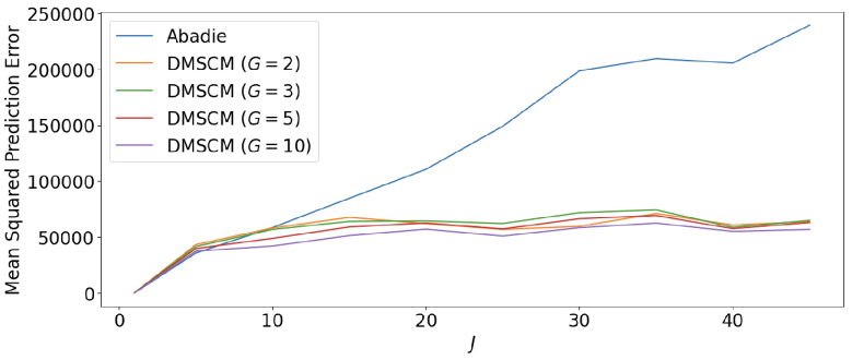
Figure 5: Results of simulation studies on ATE prediction. The $x$-axis is the number of untreated units $J$, and the $y$-axis is the mean squared prediction error.

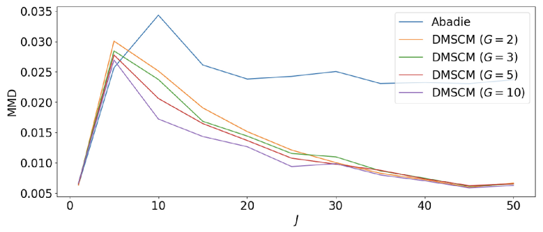
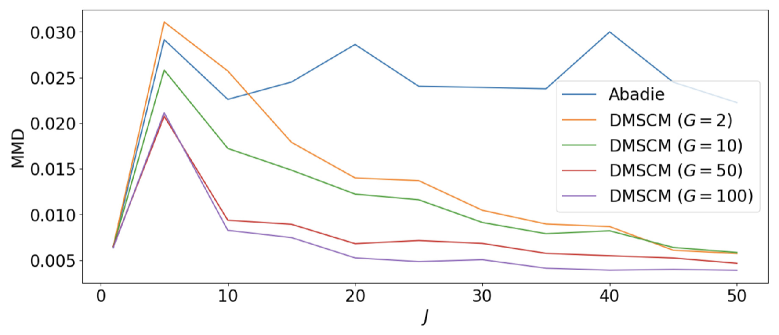
Figure 6: Results of simulation studies on DTE prediction. The $x$-axis is the number of untreated units $J$, and the $y$-axis is the MMD.

D.1 Simulation Studies

We conduct simulation studies to illustrate the comparative performance of our proposed SCMs and traditional SCMs within a setting analogous to Section 6.1. The only modifications introduced involve the parameters. Specifically, $J\in{1,5,10,15,20,\dots,35,40,45,50}$, $G\in{2,3,5,10}$, $T_{0}=30$, $T_{1}=1000$, and $K=5$. All other conditions align with those detailed in Section 6.1.

We apply DMSCM and Abadie $1,000$ times and compute the error of the ATT estimation in Figure 5. Our focus lies on the fluctuation in mean squared estimation errors as the number of units, $J$, increases. Despite the method by Abadie (2002) incurring escalating estimation errors with the increase of $J$, estimation errors do not exhibit a similar growth under our proposed methods. Furthermore, our proposed methods exhibit lower estimation errors compared to those under the method of Abadie (2002).

A comparable phenomenon is evident in DTE estimation. We compare the true and estimated distributions using the Maximum Mean Discrepancy (MMD, Gretton et al., 2012), a probability distance computed through kernel embedding. The upper figure in Figure 6 displays how MMDs alter as $J$ increases. As illustrated, our proposed methods outperform even in this task. The lower figure in Figure 6 presents results for $G\in{2,10,50,100}$. As the results indicate, the predictive capability augments as $G$ (the number of moment conditions) increases.

Our findings might have a relationship with those of Spiess et al. (2023), who investigates high-dimensional SCMs. Future investigations will be devoted to exploring these connections.

D.2 Details of Datasets

Terrorist conflict in the Basque Country.

Basque Euskadi Ta Askatasuna (Basque Homeland and Liberty; ETA) was founded in 1959 as a Basque separatist organization in Spain. ETA promoted an independent Basque state by carrying out terrorist activities mainly in the Basque Country region of Spain. Abadie & Gardeazabal (2003) utilizes annual Spanish regional-level panel data from 1955 to 1997, with a particular focus on the 1970s when ETA conducted significant terrorist activity. In the data, 15 years of pre-intervention data are included. The set of untreated units comprises $17$ other Spanish regions. Each region’s datum contains the outcome of interest (GDP per capita) at the regional level, with covariates including investment rate (percentage), population density, five sectoral productions, and four human capitals, all averaged over the period from 1955 to 1968.

Tobacco control program in California.

Abadie et al. (2010) investigate the causal effect of Proposition 99, a comprehensive tobacco control program adopted by California. They utilize annual state-level panel data from 1970 to 2000. The program was implemented in January 1989, providing 18 years of pre-intervention data. Four states that have adopted large-scale tobacco control programs (Massachusetts, Arizona, Oregon, and Florida) and states that increased state cigarette taxes by $50$ cents or more between 1989 and 2000 (Alaska, Hawaii, Maryland, Michigan, New Jersey, New York, and Washington) and the District of Columbia are excluded from the untreated units of 38 states. The outcome of interest is annual per capita cigarette consumption at the state level, measured as per capita cigarette sales in packs. Covariates include the average retail price of cigarettes, state income per capita (log), percentage of the population aged 15-24, and beer consumption per capita; all averaged over the period from 1980 to 1988.

Reunification of Germany.

Abadie et al. (2015) investigates the causal effect of the reunification of Germany. East Germany was absorbed into West Germany, the result being a reunited Germany in 1990. They utilize annual panel data at the country level from 1960 to 2003. The outcome of interest is GDP per capita at the country level. The pre-intervention period spans $30$ years. The set of untreated units comprises $16$ OECD countries that make up synthetic West Germany. Covariates include inflation rate, industry share, investment rate, schooling, and a measure of trade openness.

References

- Abadie (2002) Abadie, A. Bootstrap tests for distributional treatment effects in instrumental variable models. Journal of the American Statistical Association, 97(457):284–292, 2002.
- Abadie (2021) Abadie, A. Using synthetic controls: Feasibility, data requirements, and methodological aspects. Journal of Economic Literature, 59(2):391–425, 2021.
- Abadie & Gardeazabal (2003) Abadie, A. and Gardeazabal, J. The economic costs of conflict: A case study of the basque country. American Economic Review, 93(1):113–132, 2003.
- Abadie et al. (2010) Abadie, A., Diamond, A., and Hainmueller, J. Synthetic control methods for comparative case studies: Estimating the effect of california’s tobacco control program. Journal of the American Statistical Association, 105(490):493–505, 2010.
- Abadie et al. (2015) Abadie, A., Diamond, A., and Hainmueller, J. Comparative politics and the synthetic control method. American Journal of Political Science, 59(2):495–510, 2015.
- Athey & Imbens (2006) Athey, S. and Imbens, G. W. Identification and inference in nonlinear difference-in-differences models. Econometrica, 74(2):431–497, 2006.
- Athey & Imbens (2017) Athey, S. and Imbens, G. W. The state of applied econometrics: Causality and policy evaluation. Journal of Economic Perspectives, 31(2):3–32, 2017.
- Ben-Michael et al. (2021) Ben-Michael, E., Feller, A., and Rothstein, J. The augmented synthetic control method. Journal of the American Statistical Association, 116(536):1789–1803, 2021.
- Card & Krueger (2000) Card, D. and Krueger, A. B. Minimum wages and employment: A case study of the fast-food industry in new jersey and pennsylvania: Reply. American Economic Review, 90(5):1397–1420, 2000.
- Cattaneo et al. (2021) Cattaneo, M. D., Feng, Y., and Titiunik, R. Prediction intervals for synthetic control methods. Journal of the American Statistical Association, 116(536):1865–1880, 2021.
- Chen (2020) Chen, Y.-T. A distributional synthetic control method for policy evaluation. Journal of Applied Econometrics, 35(5):505–525, 2020.
- Chernozhukov et al. (2019) Chernozhukov, V., Wüthrich, K., and Zhu, Y. Inference on average treatment effects in aggregate panel data settings. cemmap working paper, 2019.
- Chernozhukov et al. (2021) Chernozhukov, V., Wüthrich, K., and Zhu, Y. An exact and robust conformal inference method for counterfactual and synthetic controls. Journal of the American Statistical Association, 116(536):1849–1864, 2021.
- Chikahara et al. (2022) Chikahara, Y., Yamada, M., and Kashima, H. Feature selection for discovering distributional treatment effect modifiers. In UAI, 2022.
- Cunningham & Shah (2017) Cunningham, S. and Shah, M. Decriminalizing Indoor Prostitution: Implications for Sexual Violence and Public Health. The Review of Economic Studies, 85(3):1683–1715, 2017.